[1,2]\fnmArthur \surLedaguenel
1]\orgnameIRT SystemX, \orgaddress\cityPalaiseau, \countryFrance
2]\orgdivMICS, \orgnameCentraleSupélec, \orgaddress\stateSaclay, \countryFrance
Complexity of Probabilistic Reasoning for Neurosymbolic Classification Techniques
Abstract
Neurosymbolic artificial intelligence is a growing field of research aiming to combine neural network learning capabilities with the reasoning abilities of symbolic systems. Informed multi-label classification is a sub-field of neurosymbolic AI which studies how to leverage prior knowledge to improve neural classification systems. A well known family of neurosymbolic techniques for informed classification use probabilistic reasoning to integrate this knowledge during learning, inference or both. Therefore, the asymptotic complexity of probabilistic reasoning is of cardinal importance to assess the scalability of such techniques. However, this topic is rarely tackled in the neurosymbolic literature, which can lead to a poor understanding of the limits of probabilistic neurosymbolic techniques. In this paper, we introduce a formalism for informed supervised classification tasks and techniques. We then build upon this formalism to define three abstract neurosymbolic techniques based on probabilistic reasoning. Finally, we show computational complexity results on several representation languages for prior knowledge commonly found in the neurosymbolic literature.
keywords:
Neurosymbolic, Probabilistic Reasoning, Computational complexity1 Introduction
Neurosymbolic Artificial Intelligence (AI) is a growing field of research aiming to combine neural network learning capabilities with the reasoning abilities of symbolic systems. This hybridization can take many shapes depending on how the neural and symbolic components interact, like shown in [1, 2].
An important sub-field of neurosymbolic AI is Informed Machine Learning [3], which studies how to leverage background knowledge to improve neural systems. There again, proposed techniques in the literature can be of very different nature depending on the type of task (e.g. regression, classification, detection, generation, etc.), the language used to represent the background knowledge (e.g. mathematical equations, knowledge graphs, logics, etc.), the stage at which knowledge is embedded (e.g. data processing, neural architecture design, learning procedure, inference procedure, etc.) and benefits expected from the hybridization (e.g. explainability, performance, frugality, etc.).
In this paper, we tackle supervised classification tasks informed by prior knowledge represented as a logical theory. We consider neurosymbolic techniques that integrate prior knowledge during learning, inference or both and that mainly aim at improving the performance of a neural classification system. More specifically, we study a family of neurosymbolic techniques that leverage probabilistic reasoning to integrate prior knowledge, a trend that has gained significant traction in the recent literature. In this context, the asymptotic complexity of probabilistic reasoning is of cardinal importance to assess the scalability of such probabilistic neurosymbolic techniques to large classification tasks (e.g. ImageNet dataset [4] contains 1,000 classes, and up to 1,860 when adding parent classes in the WordNet hierarchy [5], Census Cars dataset [6] contains 2,675 of cars and iNaturalist dataset [7] contains 5,089 classes of natural species). However, because neurosymbolic techniques are typically evaluated on toy datasets where complexity issues are not yet relevant and because performance metrics are the main focus, this topic is rarely tackled in the neurosymbolic literature, which can lead to a poor understanding of the applicability and limits of a given technique. For instance, [8] highlights scalability issues of existing neurosymbolic techniques on the multi-digit MNIST-addition task and propose an approximate solution, but [9] later shows that the task can be tackled in time linear in the number of digits. This is also due to a persistent lack of communication between the neurosymbolic community and the knowledge representation community. We hope this work will help to fill this gap.
The contributions and outline of the paper are as follows: we start with preliminary definitions of logics, probabilistic reasoning, and neural classification in Section 2. Then, we introduce in Section 3 a formalism to define informed supervised classification tasks and techniques. We build upon this formalism to re-frame three abstract neurosymbolic techniques that can be applied in any logic. To the best of our knowledge, we are the first to provide such a general overview of probabilistic neurosymbolic techniques for informed supervised classification. Finally, we examine in Section 4 the asymptotic computational complexity of several classes of probabilistic reasoning problems that are often encountered in the neurosymbolic literature. We show that probabilistic techniques can not scale on certain popular tasks found in the literature, whereas others thought intractable can actually be computed efficiently. We conclude with possible future research questions in Section 5.
2 Preliminaries
2.1 Logics
All logics have two sides. The syntax gives the grammar for describing the world on which the logic operates: it characterizes a set of states this world can be in and a admissible statements that can be made about the world. The semantic determines the relation between these statements and states: it specifies in which states a statement can be considered true or false.
In this paper, we focus on logics in which the states correspond to assignments from a discrete set of variables. Let’s assume a discrete set of variables , a state is an element of , where is the set of boolean values. It can be viewed either as a function that maps variables in to boolean values or as a subset of the variables. A boolean function is a an element of . It can be viewed either as a function that maps states in to boolean values or as a subset of . A boolean function can be used to represent the set of possible states given our knowledge about the world. When the set of variables is finite, we will often assume without loss of generality that with . An abstract logic can be seen as a language for expressing boolean functions on finite sets of variables in a concise way.
Definition 1 (Abstract logic).
An (abstract) logic is a couple such that for any discrete set of variables :
-
•
is the set of admissible theories on
-
•
determines which states on satisfy a theory :
When the set of variables is clear from context, we simply note and in place of and .
A logic is universal iff for any discrete set of variables any boolean function can be represented by a theory, i.e. .
We say that a logic is a fragment of a logic , noted iff for any discrete set of variables : and is the restriction of to .
A state satisfies a theory iff . We also say that accepts . A theory is satisfiable if it is satisfied by a state, i.e. if . Two theories and are equivalent iff .
We give below some examples of standard abstract logics often found in the neurosymbolic literature.
Propositional logic is the most common, typically used as an introduction to logical reasoning in many textbooks.
-
•
a propositional formula is formed inductively from variables and other formulas by using unary () or binary () connectives:
-
•
a theory in is a set of propositional formulas, i.e. or
-
•
a state inductively defines a valuation such that:
-
•
is such that:
Answer Set Programming (ASP) is one of the simplest examples of non-monotonic logics, which enable concise representations of complex knowledge at the cost of monotonicity.
-
•
formulas in are called rules and have the shape:
with . is called the head of the rule and is called the body. When the body is empty the rule can be noted .
-
•
a theory is a set of rules (i.e. ) and is called a program.
-
•
the reduct of a program relative to a state is the program such that:
To get , we first eliminate all rules in such that does not satisfy the negative part of the body, then for remaining rules, we delete the negative part of the body and add them to .
-
•
we say that a state satisfies a rule iff where:
-
•
follows the answer set semantics: a state in an answer set for a program , noted , iff it is the smaller state (in terms of inclusion) to satisfy all rules of .
Linear Programming is traditionally associated to constrained optimization problems, but it can be used to define a logic naturally suited to express many real-world problems.
-
•
formulas in are called linear constraints and have the shape:
with and . A linear constraint is sometimes noted where and .
-
•
a theory is a set of linear constraints (i.e. ) and is called a linear program.
-
•
a state satisfies a linear constraint iff in the usual arithmetical sense.
-
•
a state satisfies a linear program (i.e. ) iff it satisfies all linear constraints in .
Graph-based logics allow to reason about elements of a graph. Contrary to other logics described above, graph-based logics are not universal. They are often used to represent fragments of universal logics in a concise and more intuitive way.
-
•
a theory for a discrete set of variables is a couple where is a graph and , with , is injective.
-
•
we say that a theory is edge-based (resp. vertice-based) if (resp. ), and we note (resp. ) the set of edge-based (resp. vertice-based) theories on .
-
•
the semantics of the logic determines for a given graph if the selected elements in a state form a valid substructure of .
We give examples of graph-based logics in Sections 4.2.1, 4.2.3 and 4.2.4.
2.2 Probabilistic reasoning
One challenge of neurosymbolic AI is to bridge the gap between the discrete nature of logic and the continuous nature of neural networks. Probabilistic reasoning can provide the interface between these two realms by allowing us to reason about uncertain facts. In this section, we introduce two probabilistic reasoning problems: Probabilistic Query Estimation (PQE), i.e. computing the probability of a theory to be satisfied, and Most Probable Explanation (MPE), i.e. finding the most probable state that satisfies a given theory.
A probability distribution on a set of boolean variables is an application that maps each state to a probability such that . To define internal operations between distributions, like multiplication, we extend this definition to un-normalized distributions . The null distribution is the application that maps all states to . The partition function maps each distribution to its sum, and we note the normalized distribution (when is non-null). A boolean function is a distribution that maps all states to . The mode of a distribution is its most probable state, ie .
Typically, when belief about random variables is expressed through a probability distribution and new information is collected in the form of evidence (i.e. a partial assignment of the variables), we are interested in two things: computing the probability of such evidence and updating our beliefs using Bayes’ rules by conditioning the distribution on the evidence. Probabilistic reasoning allows us to perform the same operations with logical knowledge in place of evidence. Let’s assume a probability distribution on variables , an abstract logic and a satisfiable theory . Notice that defines a probability distribution on the set of states of and that is a boolean function on .
Definition 2.
The probability of under is:
| (1) |
The distribution conditioned on , noted , is:
| (2) |
By convention, if , then is the null-distribution. The semantic of the logic is assumed to be deduced implicitly from the context and therefore does not explicitly appear in the notations and .
A standard distribution in deep learning is the exponential distribution, which is parameterized by a vector of scores , one for each variable in . We note as a simpler notation for assuming .
Definition 3.
Given a vector , the exponential distribution is:
| (3) |
We will also note the corresponding normalized probability distribution.
The exponential probability distribution corresponds to the joint distribution of independent Bernoulli variables with , where is the sigmoid function. Since is strictly positive (for all ), if is satisfiable then its probability under is also strictly positive. We note:
Computing is a counting problem called Probabilistic Query Estimation (PQE). Computing the mode of is an optimization problem called Most Probable Explanation (MPE). Notice that computing for a satisfying state is equivalent to solving PQE because can be computed in polynomial time and:
Solving these probabilistic reasoning problems is at the core of many neurosymbolic techniques, as shown in Section 3.3.
3 Informed supervised classification
3.1 Task
In machine learning, the objective is to usually learn a functional relationship between an input domain and an output domain from data samples. Supervised multi-label classification is a subset of machine learning where input samples are labeled with subsets of a finite set of classes . Therefore, labels can be understood as states on the set of variables . In this case, the output space of the task, i.e. the set of all labels, is . In informed supervised (multi-label) classification, prior knowledge (sometimes called background knowledge) specifies which states in the output domain are semantically valid, i.e. to which states can input samples be mapped. The set of valid states constitute a boolean function on the set of variables . As shown in Section 2.1, a natural way to represent such knowledge is to use a logical theory, i.e. to provide an abstract logic and a satisfiable theory such that . For instance, hierarchical and exclusion constraints are used in [10], propositional formulas in conjunctive normal form are used in [11], boolean circuits in [12], ASP programs in [13] and linear programs in [14].
3.2 Neural classification system
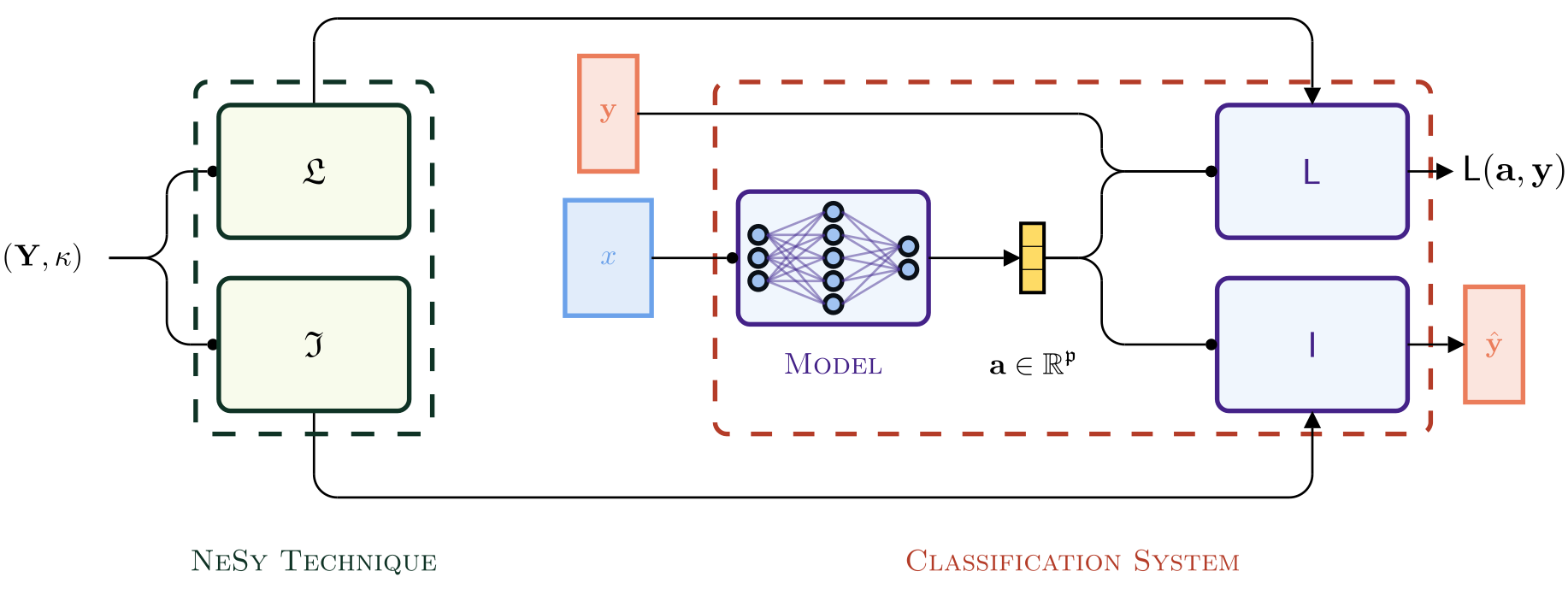
Following [15], we describe neural classification systems with three modules:
-
•
a parametric differentiable (i.e. neural) module , called the model, which takes in an input sample and parameters and produces a score for each output variable.
-
•
a non-parametric differentiable module , called the loss module, which takes the output of the model and a label and produces a positive scalar.
-
•
a non-parametric module , called the inference module, which transforms the vector of scores produced by the network into a predicted state.
The first two modules are standard in any machine learning system. The third module however, which bridges the gap between the continuous nature of the neural network (needed for backpropagation) and the discrete nature of the output space, is rarely explicitly specified.
Some neural classification systems come with a natural probabilistic interpretation. The scores produced by the model implicitly represent the parameters of a conditional probability distribution on the space of outputs . The loss module computes the negative log-likelihood of a label under that distribution. And the inference module computes the most probable output given the learned distribution.
3.3 Neurosymbolic techniques
In this paper, we assume that the architecture of the neural model (e.g. fully connected, convolutional, transformer-based, etc.) is mainly dependent on the modality of the input space (e.g. images, texts, videos, time series, etc.). Therefore we only consider neurosymbolic techniques that integrate prior knowledge in the two other modules of our neural classification system, as illustrated on Figure 1. We call such techniques model agnostic neurosymbolic techniques and give a formal definition.
Definition 4 (Neurosymbolic technique).
An abstract (model agnostic) neurosymbolic technique is such that for any abstract logic , finite set of variables and theory :
We define below three abstract neurosymbolic techniques (semantic conditioning, semantic regularization and semantic conditioning at inference) and relate each technique to the existing neurosymbolic literature.
Following the probabilistic interpretation introduced in 3.2, a natural way to integrate prior knowledge into a neural classification system is to condition the distribution on . This conditioning affects the loss and inference modules, both underpinned by the conditional distribution. It was first introduced in [10] for Hierarchical-Exclusion (HEX) graphs constraints. Semantic probabilistic layers [12] can be used to implement semantic conditioning on circuit theories. Moreover they go beyond exponential distributions and allow for a more expressive family of distributions using probabilistic circuits. NeurASP [13] defines semantic conditioning on a predicate extension of ASP programs. Likewise, DeepProbLog [16] provides an interface between Problog [17] programs and neural networks. However, since probabilistic reasoning in DeepProbLog is performed through grounding, its computational complexity is akin to that of semantic conditioning where the set of variables is the Herbrand base of the Prolog program. An approached method for semantic conditioning on linear programs is proposed in [14].
Definition 5.
Semantic conditioning is such that for any abstract logic , finite set of variables and theory :
| (4) | |||
| (5) |
An other approach and one of the most popular in the literature is to use a multi-objective scheme to train the neural network on both labeled instances and semantic constraints: a regularization term measuring the consistency of the output of the neural network with the prior knowledge is added to the standard negative log-likelihood of the labels to steer the model towards producing scores that match the background knowledge. First introduced using fuzzy logics [18, 19, 20], a regularization technique based on probabilistic reasoning was introduced for propositional theories in [11].
Definition 6.
Semantic regularization (with coefficient ) on an abstract logic is such that for any finite set of variables :
| (6) | |||
| (7) |
Finally, semantic conditioning at inference is derived from semantic conditioning, but only applies conditioning in the inference module (i.e. infers the most probable state that satisfies prior knowledge) while retaining the standard negative log-likelihood loss. It was introduced for propositional prior knowledge in [15].
Definition 7.
Semantic conditioning at inference is such that for any abstract logic , finite set of variables and theory :
| (8) | |||
| (9) |
4 Complexity
As mentioned in Section 2.2, all three abstract neurosymbolic techniques defined in Section 3.3 rely on solving MPE and PQE problems. Unfortunately, in the general cases of propositional logic, answer set programming and linear programming, MPE and PQE are NP-hard and #P-hard respectively. This implies that scaling these probabilistic neurosymbolic techniques to large classification tasks (i.e. tasks with a large number of variables) on arbitrary prior knowledge requires an exponential amount of computing resources (under the assumption that ) and is therefore not realistic. However, there are fragments of these universal logics for which probabilistic reasoning problems can be solved efficiently. Hence, it is crucial to understand more finely the computational complexity of probabilistic reasoning to assess the scalability and limitations of such techniques.
We first mention in Section 4.1 two popular families of algorithms for solving PQE and MPE problems, based on graphical models and knowledge compilation respectively. Then, we analyze in Section 4.2 the complexity of several classes of MPE and PQE problems that are frequently encountered in the neurosymbolic literature.
4.1 Algorithms
4.1.1 Graphical models
Graphical models allow to specify a family of distributions over a finite set of variables by means of a graph. The graph encodes a set of properties (e.g. factorization, independence, etc.) shared by all distributions in the family. These properties can be exploited to produce compressed representations and efficient inference algorithms. In the context of probabilistic reasoning, the primal graph of a theory specifies to which graphical model the family of exponential distributions conditioned on belong. In particular, traditional algorithms for graphical models can be leveraged to solve PQE and MPE problems in time where is the number of variables and the treewidth of the primal graph of . Such algorithms were used to implement semantic conditioning in [10].
4.1.2 Knowledge compilation
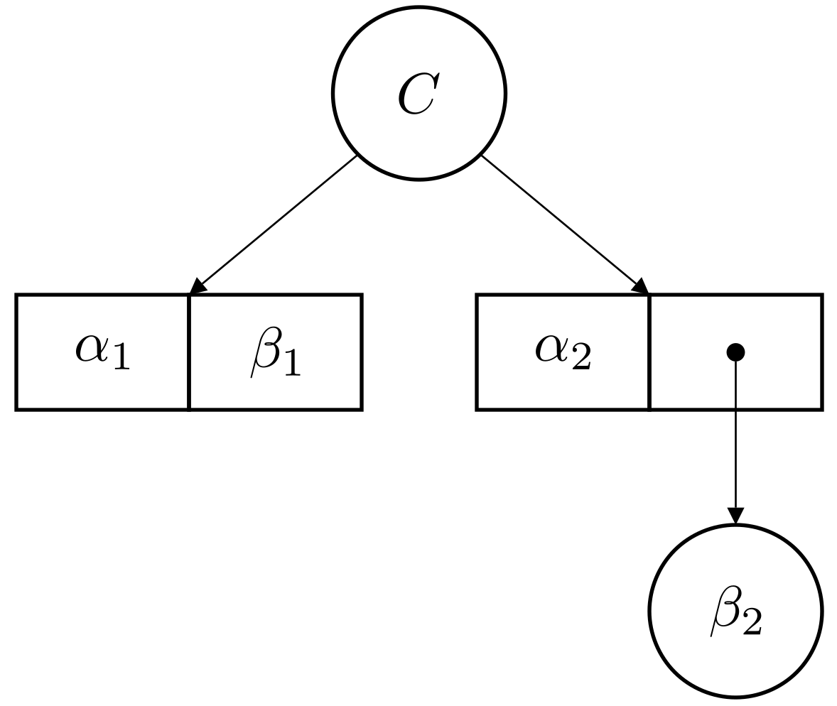
Knowledge compilation is the process of translating theories from a given representation logic (e.g. conjunctive normal form) into a target logic that supports some operations efficiently. Several fragments of boolean circuits [21] were identified as suitable target logics. Decomposable Negational Normal Form (DNNF) circuits can solve MPE problems in linear time (in the size of the circuit) and deterministic-DNNF can solve PQE problems in linear time. Sentential Decision Diagrams (SDD) [22] is a PQE and MPE-tractable fragment of boolean circuits [21] that offers linear and polynomial negation, conjunction and disjunction. Besides, [22] shows that a propositional formula in conjunctive normal form with variables and a tree-width has an equivalent compressed and trimmed SDD of size . Due to these properties, SDD has become a standard target logic for probabilistic neurosymbolic systems [11, 12]. In this paper, we use the graphical representation in [22] to represent SDD nodes. For instance, the node represented in Figure 2 is equivalent to where are terminal nodes (i.e. literals, or ) and is another SDD node (structured according to the same linear vtree).
4.2 Tractable logics
An abstract logic is concise if the size of its theories on finite sets of variables is polynomial in the number of variables. Edge-based (resp. vertice-based) logics (see Section 2.1) are concise by design: since has to be injective, the number of edges (resp. vertices) in the graph cannot be larger than the number of variables. A logic is MPE-tractable (resp. PQE-tractable) if MPE problems (resp. PQE problems) for a theory can be solved in time polynomial in the size of the theory. A logic is tractable if it is concise, MPE and PQE-tractable. Moreover, counting problems are known to be much harder in general than optimization problems [23]. Therefore, it is natural to look for logics which are concise, MPE-tractable and for which PQE is still #P-hard. We call them semi-tractable logics. Besides the theoretical interest, these logics have great relevance in the context of probabilistic neurosymbolic techniques, as some remain scalable on semi-tractable logics (e.g. semantic conditioning at inference) while others do not (e.g. semantic conditioning and semantic regularization).
As mentioned earlier, a typical criteria to identify a tractable fragment is to show that it is bounded in tree-width. However, most prior knowledge commonly found in the neurosymbolic literature do not meet this criteria. Therefore, in this section, we analyze the complexity of MPE and PQE problems for several logics of unbounded tree-width. A summary of the results can be found in Table 1. We tackle hierarchical classification [10, 12] in Section 4.2.1. Fixed cardinal constraints (or k-subset constraints) are mentioned in [14] as an example of computationally hard constraints for PQE. However, we give tractability results for such constraints in Section 4.2.2. Simple path constraints are growing increasingly popular in the neurosymbolic literature [11, 24, 14, 12, 25]. We show in Section 4.2.3 that simple path constraints are intractable in general, but that restricting to acyclic graphs render them tractable, meaning that probabilistic techniques can scale on acyclic graphs. It is worth noting that most techniques in the field are illustrated on grid graphs, which contain cycles. Informed classification tasks with matching constraints can be found in [24, 25]. We show that matching theories are semi-tractable in Section 4.2.4.
| Logics | Bounded treewidth | MPE | PQE |
|---|---|---|---|
| General | ✗ | ✗ | ✗ |
| Tree-like hiearchical | ✓ | ✓ | ✓ |
| Hierarchical with mutual exclusion | ✗ | ✓ | ✓ |
| Fixed cardinal | ✗ | ✓ | ✓ |
| Simple path in directed graphs | ✗ | ✗ | ✗ |
| Acyclic simple path | ✗ | ✓ | ✓ |
| Matchings | ✗ | ✓ | ✗ |
4.2.1 Hierarchical
Hierarchical constraints (e.g. a dog is an animal) are ubiquitous in artificial intelligence because we are used to organize concepts in taxonomies, so much so that hierarchical classification (i.e. a classification task where the set of output classes are organized in a hierarchy) is a field of research on its own.
Hierarchical logic is a vertex-based logic where a theory accepts a state (i.e. ) if the vertices selected in respect the hierarchical constraints expressed in : if a vertex belong to an accepting state (i.e. ), then all its parents in also belong to .
A hierarchical theory of can be compiled in polynomial time in a 2-cnf formula:
| (10) |
Proposition 1.
The fragment of hierarchical logic composed of theories where is a tree is tractable.
Proof.
defined in Equation 10 is a 2-cnf of treewidth 1. Therefore can be compiled into an SDD of size polynomial in . ∎
The semantics of hierarchical logic can be changed to so that variables that have no common descendants in are considered mutually exclusive: if belong to an accepting state (i.e. ) and is such that there is no directed path from to or from to , then does not belong to (i.e. ).
Proposition 2.
Hierarchical logic with mutual exclusion assumptions is tractable.
Proof.
Theories in are enumerable. For each vertex , the state that contains and its ancestors is accepted by . The null state is the only other state accepted by . Therefore, accepted states can be enumerated in polynomial time in the size of the theory. This means that PQE can be solved by summing probabilities of satisfying states. Likewise, MPE can be solved by iterating through satisfying states to find the most probable one. Hence, hierarchical logic with mutual exclusion assumptions is tractable. ∎
4.2.2 Fixed cardinal
Fixed cardinal constraints can be used to represent a classification task which consists in picking a fixed amount of variables in a given list (e.g. suggesting a given number of related products to a client).
A fixed cardinal theory consists of a linear constraint which accepts states that contain exactly variables amongst a set of size (ie. states such that ).
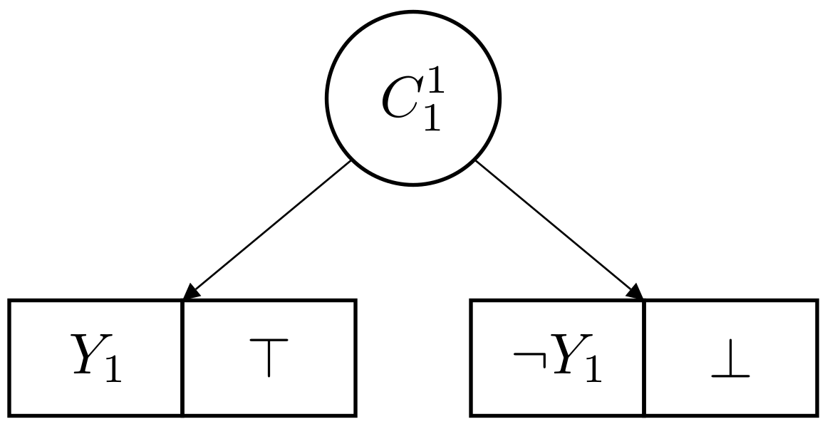
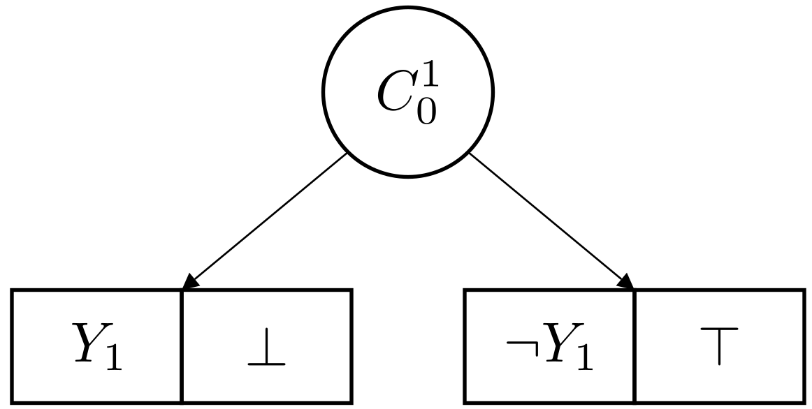
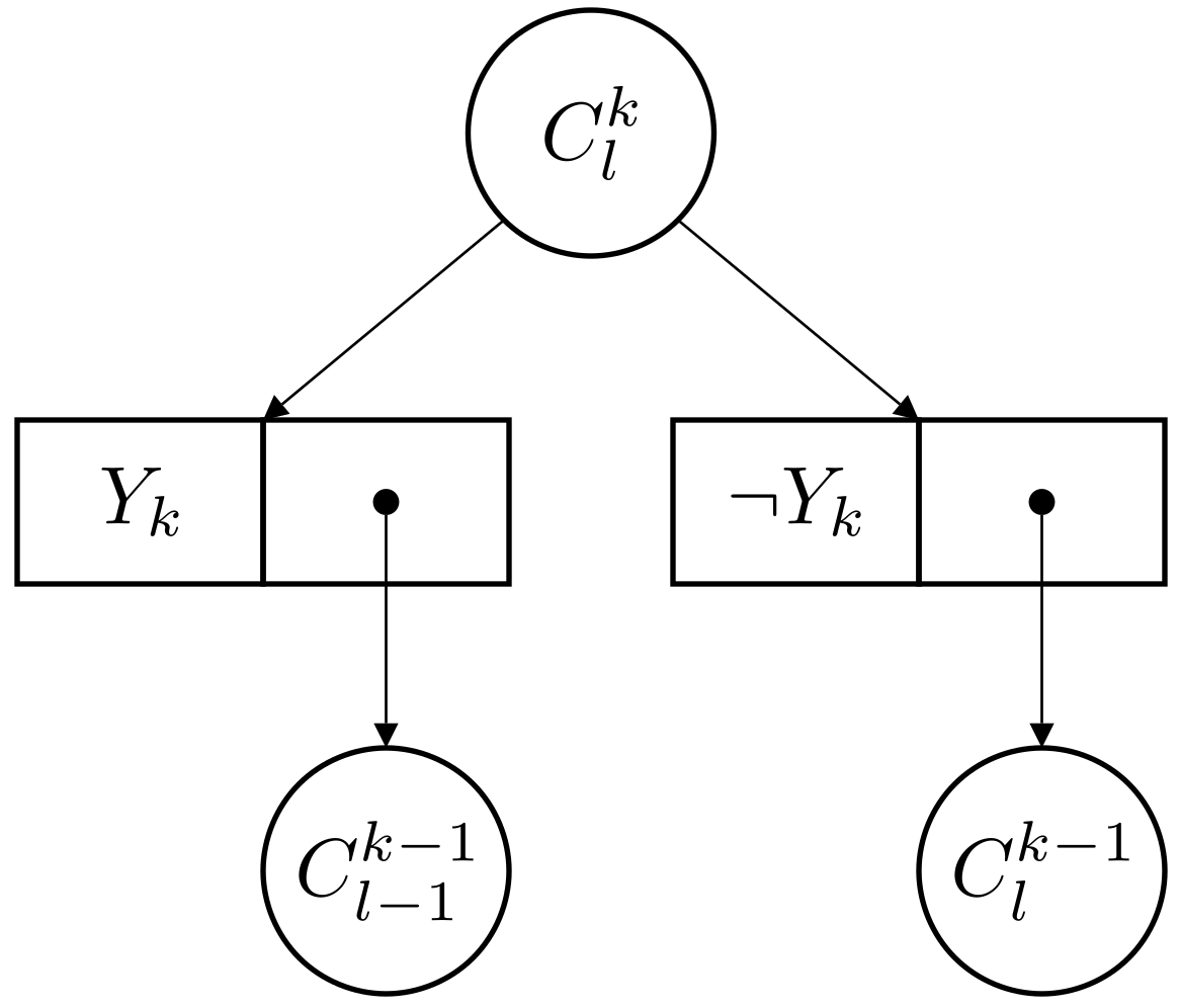
Figures 3 gives a recursive template (using the graphical representation in [22]) to compile in polynomial time (create all decision nodes and connect them appropriately) a fixed cardinal theory into a concise SDD.
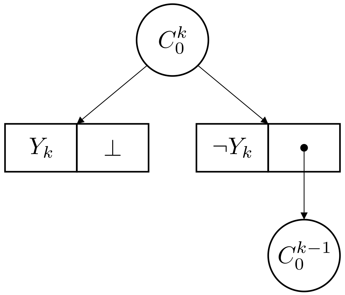
Proposition 3.
Circuit has size polynomial in .
Proof.
Circuit contains nodes with wires each, meaning that the size of the circuit is in . ∎
Proposition 4.
For any number of variables and the circuit rooted in is a SDD (and even an OBDD) structured according to the right linear vtree on .
Proof.
Proof by recurrence on starting at :
-
•
Initialization for : and only contains variable and thus is structured according to the right linear vtree on .
-
•
Heredity from to : for all , has primes and subs if and if which are all structured according to the right linear vtree on , hence is structured according to the right linear vtree on .
∎
Proposition 5.
The circuit with and accepts a state iff it contains exactly variables (ie. ).
Proof.
Proof by recurrence on starting at :
-
•
Initialization for : only accepts and only accepts .
-
•
Heredity from to , for and :
-
–
if : iff and , which means accepts iff:
-
–
if : in only two cases:
-
*
if and , which means we have:
-
*
if and , which means we have:
-
*
-
–
∎
4.2.3 Simple paths
The task of Warcraft Shortest Path [24] is to learn how to predict the shortest path on a map from a picture of the map. Such a task can be viewed as an informed classification task where the set of output variables correspond to edges in a graph and prior knowledge informs us that only states representing simple paths in the graph are satisfying answers.
Simple path logic is an edge-based logic where a theory accepts a state if the edges selected in (ie. ) form a s-t simple path in , i.e. if the selected edges forms an acyclic path from a source of the graph to a target (or sink) of the graph.
Proposition 6.
Simple path logic is MPE and PQE-intractable.
Proof.
Solving MPE for a simple path theory is equivalent to finding a shortest path in with real weights on the edges, which is known to be NP-hard by a polynomial reduction from the Hamiltonian path problem [26]. Likewise, counting the number of simple paths of a graph is known to be #P-hard [27] and has a trivial polynomial reduction to solving PQE for a simple path theory . ∎
A simple path theory is said acyclic if is a Directed Acyclic Graph (DAG). We say that is topological if is a topological ordering of the edges: for any path, the order of edges in the path is a sub-order of the topological order. For a vertex , we will note the index of the first incident edge to and the index of the last outgoing edge of . We also note the graph that contains edges and all vertices that are endpoints of those edges. Finally, we can assume without loss of generality that only contains a single source and target. If not: chose one source vertex , delete all the others and reconnect their outgoing edges to , and do the same with a target vertex . This operation can be done in polynomial type and does not change the semantic of the theory (i.e. accepted states are left unchanged).
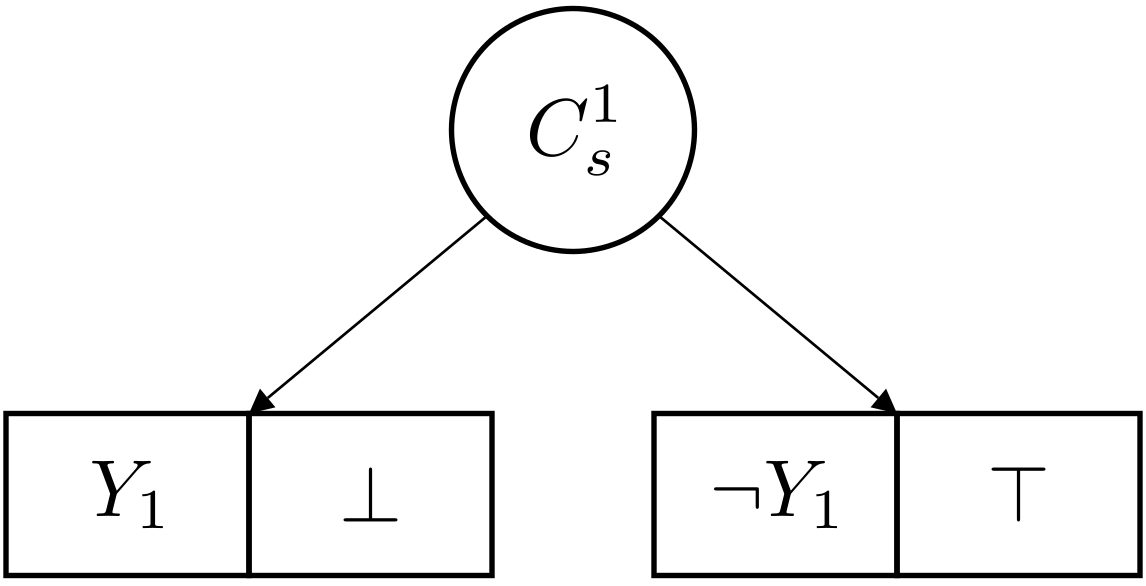
Figures 4 and 5 represent recursive templates that allow us to compile in polynomial time (create all decision nodes and connect them appropriately) an acyclic and topological simple path theory into a concise SDD rooted in node .

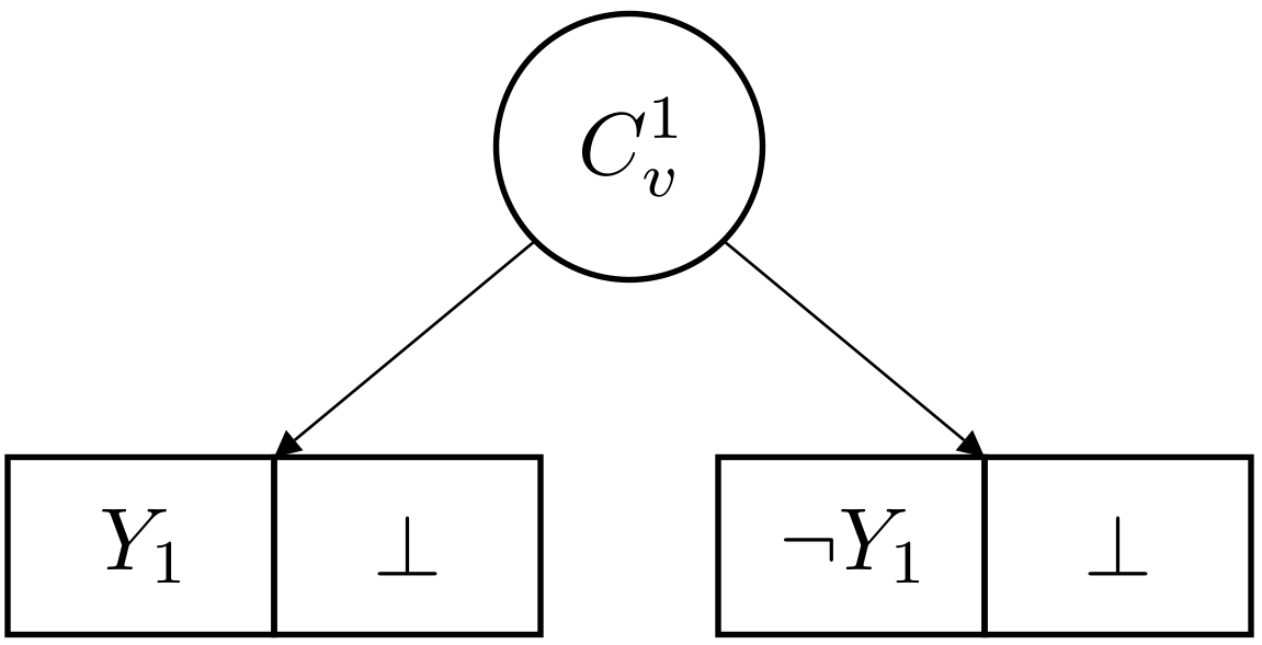
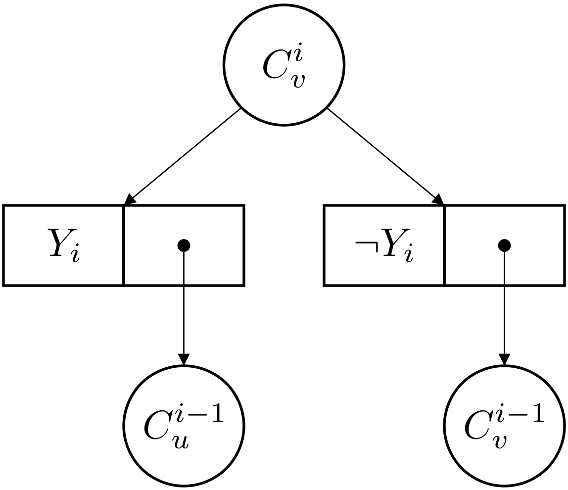
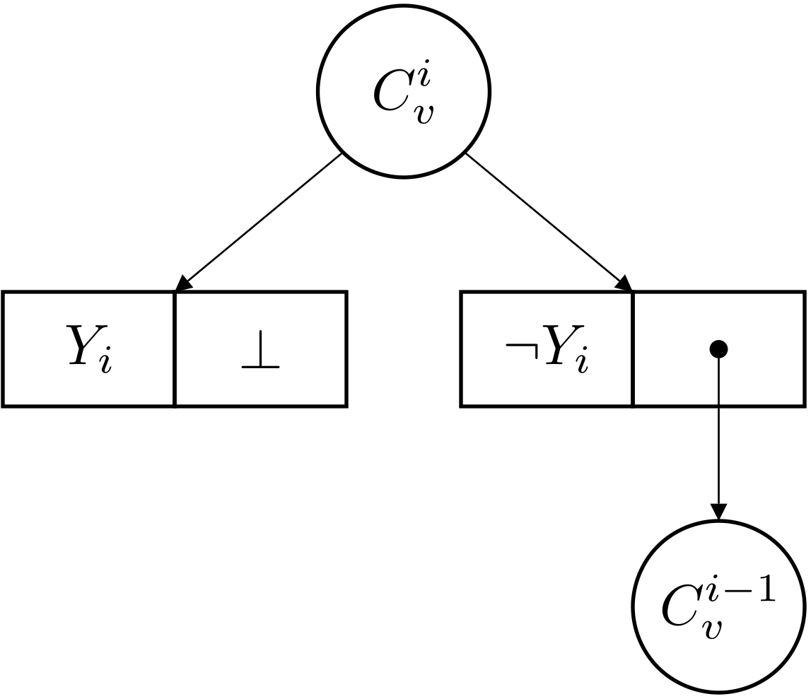
Proposition 7.
Circuit has size polynomial in the number of edges in .
Proof.
Circuit has at most decision nodes with wires each, meaning that the size of the circuit is in . ∎
Remark 1.
Notice that every node such that such that will not appear in the circuit rooted in . Similarly, every node such that is equivalent to and can thus be trimmed of the circuit. Therefore, the size of the trimmed circuit is much smaller that .
Proposition 8.
For each vertex and edge , the circuit rooted in is a SDD (and even an OBDD) structured according to the right linear vtree on .
Proof.
Proof by recurrence on :
-
•
Initialization for : for all vertices , only contains variable and thus is structured according to the right linear vtree on .
-
•
Heredity from to : for all vertices , has primes and subs which are all structured according to the right linear vtree on , hence is structured according to the right linear vtree on .
∎
Lemma 9.
Assume that edges follow a topological order. If for represents a path in and , then for some .
Proof.
We note . We first show that :
-
•
if , then .
-
•
if , since represents a path , there is an edge with , which means that .
Now let’s show that reasoning by the absurd. Let’s assume that , then since represents a path , there is an edge with . Hence, there is a path from the end point of to the start point of with , which is in contradiction with edges following a topological order.
Therefore we can conclude that for some . ∎
Lemma 10.
The circuit with only accepts the null state .
Proof.
Proof by recurrence on :
-
•
Initialization for : iff by definition (see Figure 4(c)).
-
•
Heredity from to : has no incoming edge in (because it is a source vertex), hence accepts iff and . Which means by the recurrence hypothesis that and therefore .
∎
Proposition 11.
The circuit with and accepts a state iff it is a path in . In particular represents .
Proof.
We will proceed by recurrence on , first showing that all accepted states by are paths in then showing that only them are accepted.
-
•
Initialization for : only contains the vertices and such that and accepts exactly which is the only path in .
-
•
Heredity from to :
- –
-
–
Assume a state is accepted by :
- *
-
*
if , then , hence by the recurrence hypothesis represents a path in and by not adding edge represents a path in .
∎
Finally, we can state our main result:
Proposition 12.
The fragment of simple path logic composed of acyclic theories is tractable.
Proof.
First, it is concise because it is an edge-based logic. Let’s assume an acyclic simple path theory . If needed, merge source vertices and target vertices like mentioned above. Since a topological order of the edges in a DAG can be compiled in a polynomial time, we can compute such that is acyclic and topological. We compile into a concise SDD as seen above. We rewrite leaf nodes to in the SDD. The new circuit is still a concise SDD, structured according to the right linear vtree on and is equivalent to the theory . Because SDD is MPE and PQE-tractable, we have that acyclic simple path logic is concise, MPE and PQE-tractable. Therefore, acyclic simple path logic is tractable. ∎
4.2.4 Matchings
Matching problems naturally arise in artificial intelligence when one wants to find the best pairing between various entities (e.g. individuals, tasks, resources, etc.). A matching task can be thought of as an informed classification task where classes correspond to edges in a graph and prior knowledge tells us that only states that represent a matching (i.e. a set of non-adjacent edges) are accepted.
Matching logic is an edge-based logic where a theory accepts a state if the edges selected in correspond to a matching in (i.e. no vertex in has two adjacent edges in ). Notice that matching logics ignore the direction of edges.
Matching theories can be compiled in 2-cnf formulas with:
| (11) |
Proposition 13.
Matching logic is semi-tractable.
5 Conclusion
In this paper, we introduced an abstract formalism for informed supervised classification tasks and techniques (Section 3). To the best of our knowledge, we are the first to provide such a general view that capture prior knowledge expressed in any abstract logic (e.g. propositional logic, answer set programming or linear programming). We build upon this formalism to re-frame three abstract neurosymbolic techniques based on probabilistic reasoning and relate them to various papers that defined them in the context of specific logics. Finally, we study the computational complexity of probabilistic reasoning for several families of prior knowledge commonly found in the neurosymbolic literature (Section 4). We showed for instance that some families of logical constraints that were thought computationally hard are actually scalable, while others that are frequently used in toy datasets to evaluate probabilistic neurosymbolic techniques are not. We also established that there are logics for which some techniques are tractable (e.g. semantic conditioning at inference) while others are not (e.g. semantic conditioning and semantic regularization), introducing a new criteria of comparison for probabilistic neurosymbolic techniques.
Future directions for our research include a sharper understanding of semi-tractable logics and their practical consequences for informed classification tasks. We would like to explore approximate methods for probabilistic neurosymbolic techniques, in the case where prior knowledge is intractable. Finally, we are also interested in expanding our formalism beyond supervised classification to semi-supervised and weakly-supervised settings.
References
- \bibcommenthead
- Kautz [2022] Kautz, H.A.: The third ai summer: Aaai robert s. engelmore memorial lecture. AI Mag. 43, 93–104 (2022)
- Wang et al. [2023] Wang, W., Yang, Y., Wu, F.: Towards Data-and Knowledge-Driven Artificial Intelligence: A Survey on Neuro-Symbolic Computing (2023). https://arxiv.org/abs/2210.15889
- von Rueden et al. [2023] Rueden, L., Mayer, S., Beckh, K., Georgiev, B., Giesselbach, S., Heese, R., Kirsch, B., Pfrommer, J., Pick, A., Ramamurthy, R., Walczak, M., Garcke, J., Bauckhage, C., Schuecker, J.: Informed Machine Learning – A Taxonomy and Survey of Integrating Prior Knowledge into Learning Systems. IEEE Transactions on Knowledge and Data Engineering 35(1), 614–633 (2023) https://doi.org/10.1109/TKDE.2021.3079836 . Conference Name: IEEE Transactions on Knowledge and Data Engineering
- Russakovsky et al. [2015] Russakovsky, O., Deng, J., Su, H., Krause, J., Satheesh, S., Ma, S., Huang, Z., Karpathy, A., Khosla, A., Bernstein, M., Berg, A.C., Fei-Fei, L.: Imagenet large scale visual recognition challenge. International Journal of Computer Vision 115, 211–252 (2015) https://doi.org/10.1007/s11263-015-0816-y
- Miller [1995] Miller, G.A.: Wordnet. Communications of the ACM 38, 39–41 (1995) https://doi.org/10.1145/219717.219748
- [6] Gebru, T., Krause, J., Wang, Y., Chen, D., Deng, J., Fei-Fei, L.: Fine-grained car detection for visual census estimation 31(1) https://doi.org/10.1609/aaai.v31i1.11174 . Number: 1. Accessed 2024-03-31
- Van Horn et al. [2018] Van Horn, G., Mac Aodha, O., Song, Y., Cui, Y., Sun, C., Shepard, A., Adam, H., Perona, P., Belongie, S.: The inaturalist species classification and detection dataset. In: 2018 IEEE/CVF Conference on Computer Vision and Pattern Recognition, pp. 8769–8778 (2018). https://doi.org/10.1109/CVPR.2018.00914
- van Krieken et al. [2022] Krieken, E., Thanapalasingam, T., Tomczak, J.M., Harmelen, F., Teije, A.: A-NeSI: A Scalable Approximate Method for Probabilistic Neurosymbolic Inference (2022)
- [9] Maene, J., De Raedt, L.: Soft-unification in deep probabilistic logic 36. Accessed 2024-02-21
- Deng et al. [2014] Deng, J., Ding, N., Jia, Y., Frome, A., Murphy, K., Bengio, S., Li, Y., Neven, H., Adam, H.: Large-Scale Object Classification Using Label Relation Graphs. In: Computer Vision – ECCV 2014, pp. 48–64. Springer, ??? (2014)
- Xu et al. [2018] Xu, J., Zhang, Z., Friedman, T., Liang, Y., Broeck, G.V.D.: A semantic loss function for deep learning with symbolic knowledge. In: 35th International Conference on Machine Learning, ICML 2018, vol. 12, pp. 8752–8760. International Machine Learning Society (IMLS), ??? (2018)
- Ahmed et al. [2022] Ahmed, K., Teso, S., Chang, K.-W., Broeck, G., Vergari, A.: Semantic Probabilistic Layers for Neuro-Symbolic Learning. In: Advances in Neural Information Processing Systems, vol. 35, pp. 29944–29959. Curran Associates, Inc., ??? (2022)
- [13] Yang, Z., Ishay, A., Lee, J.: NeurASP: Embracing neural networks into answer set programming. In: Proceedings of the Twenty-Ninth International Joint Conference on Artificial Intelligence, pp. 1755–1762. International Joint Conferences on Artificial Intelligence Organization. https://doi.org/10.24963/ijcai.2020/243
- Niepert et al. [2021] Niepert, M., Minervini, P., Franceschi, L.: Implicit MLE: Backpropagating through discrete exponential family distributions. In: Advances in Neural Information Processing Systems, vol. 34, pp. 14567–14579. Curran Associates, Inc., ??? (2021). https://proceedings.neurips.cc/paper_files/paper/2021/hash/7a430339c10c642c4b2251756fd1b484-Abstract.html Accessed 2024-01-17
- Ledaguenel et al. [2024] Ledaguenel, A., Hudelot, C., Khouadjia, M.: Improving Neural-based Classification with Logical Background Knowledge (2024). https://arxiv.org/abs/2402.13019
- Manhaeve et al. [2021] Manhaeve, R., Dumančić, S., Kimmig, A., Demeester, T., De Raedt, L.: Neural probabilistic logic programming in DeepProbLog. Artificial Intelligence 298, 103504 (2021) https://doi.org/10.1016/j.artint.2021.103504 . Accessed 2023-08-07
- De Raedt et al. [2007] De Raedt, L., Kimmig, A., Toivonen, H.: ProbLog: a probabilistic prolog and its application in link discovery. In: Proceedings of the 20th International Joint Conference on Artifical Intelligence. IJCAI’07, pp. 2468–2473. Morgan Kaufmann Publishers Inc., San Francisco, CA, USA (2007)
- Diligenti et al. [2017] Diligenti, M., Gori, M., Saccà, C.: Semantic-based regularization for learning and inference. Artificial Intelligence 244, 143–165 (2017) https://doi.org/10.1016/j.artint.2015.08.011
- Giannini et al. [2023] Giannini, F., Diligenti, M., Maggini, M., Gori, M., Marra, G.: T-norms driven loss functions for machine learning. Applied Intelligence 53(15), 18775–18789 (2023) https://doi.org/10.1007/s10489-022-04383-6 . Accessed 2023-08-07
- Badreddine et al. [2022] Badreddine, S., Garcez, A.d., Serafini, L., Spranger, M.: Logic Tensor Networks. Artificial Intelligence 303, 103649 (2022) https://doi.org/10.1016/j.artint.2021.103649
- [21] Darwiche, A., Marquis, P.: A knowledge compilation map 17(1), 229–264
- Darwiche [2011] Darwiche, A.: SDD: A New Canonical Representation of Propositional Knowledge Bases. In: Proceedings of the Twenty-Second International Joint Conference on Artificial Intelligence (2011)
- Toda [1991] Toda, S.: PP is as hard as the polynomial-time hierarchy. SIAM Journal on Computing 20(5), 865–877 (1991) https://doi.org/10.1137/0220053 . Publisher: Society for Industrial and Applied Mathematics. Accessed 2024-01-17
- Pogančić et al. [2019] Pogančić, M.V., Paulus, A., Musil, V., Martius, G., Rolinek, M.: Differentiation of Blackbox Combinatorial Solvers. (2019). https://openreview.net/forum?id=BkevoJSYPB Accessed 2023-10-27
- Ahmed et al. [2022] Ahmed, K., Wang, E., Chang, K.-W., Broeck, G.: Neuro-symbolic entropy regularization. In: Cussens, J., Zhang, K. (eds.) Proceedings of the Thirty-Eighth Conference on Uncertainty in Artificial Intelligence. Proceedings of Machine Learning Research, vol. 180, pp. 43–53. PMLR, ??? (2022). https://proceedings.mlr.press/v180/ahmed22a.html
- [26] Karp, R.M.: Reducibility among combinatorial problems. In: Miller, R.E., Thatcher, J.W., Bohlinger, J.D. (eds.) Complexity of Computer Computations: Proceedings of a Symposium on the Complexity of Computer Computations, Held March 20–22, 1972, at the IBM Thomas J. Watson Research Center, Yorktown Heights, New York, and Sponsored by the Office of Naval Research, Mathematics Program, IBM World Trade Corporation, and the IBM Research Mathematical Sciences Department. The IBM Research Symposia Series, pp. 85–103. Springer. https://doi.org/10.1007/978-1-4684-2001-2_9 . https://doi.org/10.1007/978-1-4684-2001-2_9 Accessed 2024-03-11
- [27] Valiant, L.G.: The complexity of enumeration and reliability problems 8(3), 410–421 https://doi.org/10.1137/0208032 . Accessed 2024-02-21
- [28] Edmonds, J.: Maximum matching and a polyhedron with 0,1-vertices 69B(1), https://doi.org/10.6028/jres.069b.013 . Number: 1 and 2. Accessed 2024-03-11
- [29] Amarilli, A., Monet, M.: Weighted Counting of Matchings in Unbounded-Treewidth Graph Families. arXiv. https://doi.org/10.48550/arXiv.2205.00851 . http://arxiv.org/abs/2205.00851 Accessed 2024-03-11