Collective Bayesian Decision-Making in a Swarm of Miniaturized Robots for Surface Inspection

Abstract

Robot swarms can effectively serve a variety of sensing and inspection applications. Certain inspection tasks require a binary classification decision. This work presents an experimental setup for a surface inspection task based on vibration sensing and studies a Bayesian two-outcome decision-making algorithm in a swarm of miniaturized wheeled robots. The robots are tasked with individually inspecting and collectively classifying a $1m\times 1m$ tiled surface consisting of vibrating and non-vibrating tiles based on the majority type of tiles. The robots sense vibrations using onboard IMUs and perform collision avoidance using a set of IR sensors. We develop a simulation and optimization framework leveraging the Webots robotic simulator and a Particle Swarm Optimization (PSO) method. We consider two existing information sharing strategies and propose a new one that allows the swarm to rapidly reach accurate classification decisions. We first find optimal parameters that allow efficient sampling in simulation and then evaluate our proposed strategy against the two existing ones using 100 randomized simulation and 10 real experiments. We find that our proposed method compels the swarm to make decisions at an accelerated rate, with an improvement of up to 20.52% in mean decision time at only 0.78% loss in accuracy.

1 Introduction

Over the last few decades, automated inspection systems have increasingly become a valuable tool across various industries [6, 22, 23, 5]. Studies have addressed applications in agricultural and hull inspection as well as infrastructure and wind-turbine maintenance [7, 18, 17, 15]. Vibration analysis is a valuable tool in these inspection processes. Different types of vibration analysis are used to detect the condition of infrastructure through structural properties such as modal shapes and eigenfrequencies [2, 19, 10]. Certain inspection processes incorporate regression analysis, while other require making a binary classification decision [24]. A class of inspection tasks involves making a binary decision about a spatially distributed feature of the inspected system. This type of decisions can be effectively addressed by a swarm of robots. Swarms improve the decision time and accuracy of by leveraging collective perception [26, 27]. Moreover, swarms eliminate the problem of sensor-placement and can provide a high-resolution map of the environment [3, 4]. Collective decision-making algorithms often draw inspiration from nature, such as groups of ants and bees [25]. A more mathematical approach is found in Bayesian algorithms. Applications of Bayesian algorithms have been studied in sensor networks [1, 20] as well as robot swarms [26, 12, 27, 11, 14]. In the study outlined in [11], a collective of agents must determine whether the predominant color of a checkered pattern is black or white. The robots function as Bayesian modellers, exchanging information based on two information sharing strategies. The robots either (i) continuously broadcast their ongoing binary observations (no feedback strategy) or (ii) continuously broadcast their irreversible decisions once reached (positive feedback strategy).

In this work, we build on top of the work in [11] in three ways. First, we move away from the agent-based simulation and present a real experimental setup built around 3-cm-sized vibration sensing wheeled robots and utilize vibration signals in the presence of measurement noise in place of simulated binary floor color observations. We develop a new sensor board to allow the robots to perform collision avoidance. Second, we develop a simulation framework in the physics-based robotic simulator Webots and employ a Particle Swarm Optimization (PSO) method to heuristically optimize the sampling behavior of the swarm across our experimental setup, similar to [8]. We show calibration of our simulation world against our real experimental setup. Third, we present a new information sharing strategy, termed soft-feedback, leveraging the stability of no feedback and coercion of positive feedback strategies. The advantages lie in its ability to drive the swarm towards consensus, particularly in difficult to classify and noisy environments. We use simulation and experimental studies to evaluate the swarm’s performance for all three information sharing strategies and consider decision time and accuracy as metrics in our assessments.

2 Problem Definition

We task a swarm of $N$ robots to individually inspect and collectively classify a 2D tiled surface section. The surface comprises two types of tiles, vibrating and non-vibrating tiles. The swarm must determine whether the tiled surface is majority vibrating or majority non-vibrating. We denote the fill-ratio $f$ as the proportion of vibrating tiles. The robots each individually inspect the surface, share their information with the rest of the swarm, and collectively classify the surface. The inspection task ends when every robot in the swarm reaches a final decision, determining if the fill-ratio is above or below 0.5. An underlying real-world scenario could involve inspecting a surface section and determining whether the surface is in a majority healthy or in a majority unhealthy state.

3 Real Experimental Setup

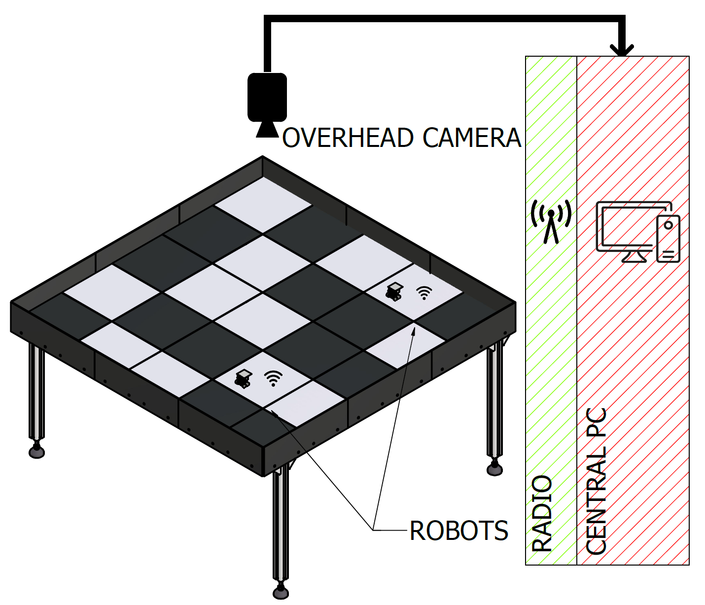
(a) Overall experimental setup.

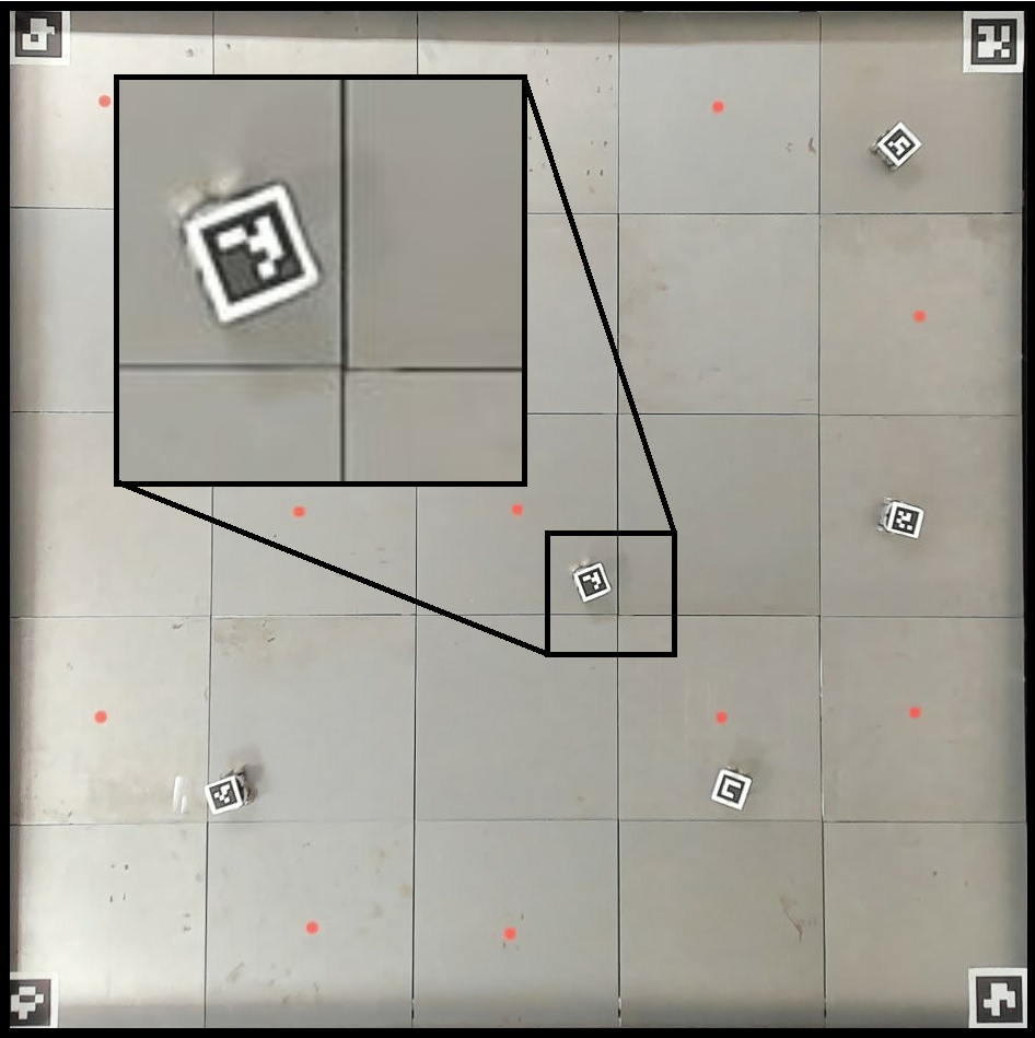
(b) View from overhead camera.

Figure 1: The experimental setup with a fill ratio of $f=\frac{12}{25}=0.48$. (a) Schematic overview of the setup is shown. The central PC uses the radio and camera data for analysis. Vibration-motors are attached on the bottom side of white tiles. (b) A snapshot from the overhead camera with detailed view (black square). The red dots indicate vibrating tiles. Each robot carries a unique AruCo marker for tracking. AruCo markers in the corners of the environment mark the boundaries.

Our experimental setup, shown in Figure 1, is built around (i) a tiled surface section of size $1m\times 1m$, and (ii) a swarm of $3cm$-sized vibration-sensing wheeled robots that traverse and inspect the tiled surface section. The surface section consists of 25 tiles, each of size $20cm\times 20cm$, that are laid out in a square grid with five tiles on each side. There are two types of tiles on the surface, vibrating and non-vibrating tiles. The vibrating tiles are excited using two miniature vibration motors mounted on top of one another underneath the tile at its center (ERM 3V Seeed Technology motors). All tiles are secured to an aluminium frame using $2cm\times 1cm$ pieces of magnetic tape around the corners. The frame consists of four strut profiles in the middle and four others along the edges of the arena. We use an overhead camera (Logitech BRIO 4k) and AruCo markers for visual tracking of the robots.

We use a revised and extended version of the Rovable robot originally presented in [9]. As shown in Figure 2, each robot measures $25mm\times 33mm\times 35mm$ and carries two customized Printed Circuit Boards (PCBs): (i) a main PCB hosting the micro-controller, an IMU, motor controllers, power circuitry and radio and (ii) an extension PCB hosting IR sensors for collision avoidance. The main PCB has essentially the same design as the one in [9], and was only revised and remade for updated components. The extension PCB is new and hosts three small Time-of-Flight (ToF) IR sensor boards, each facing a direction of $0^{\degree}$, $25^{\degree}$, and $-25^{\degree}$ relative to the forward driving direction of the robot. Each sensor has a field of view of $27^{\degree}$ and a range of up to $1m$. A 3D printed shield is mounted around the extension PCB to enhance the visibility of the robot when perceived by the IR sensors of other robots. The robot has four magnetic wheels. Only two wheels, one on the front and one on the back, are driven by PWM operated motors. At 100% PWM, the robot drives forward at around $5cm$ per second.

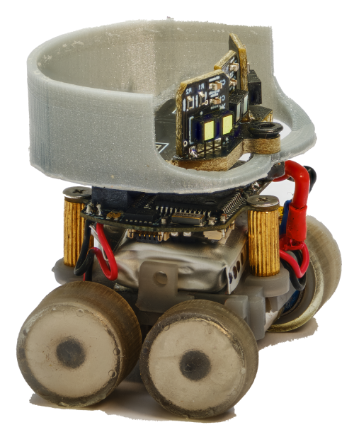
(a) Extended robot

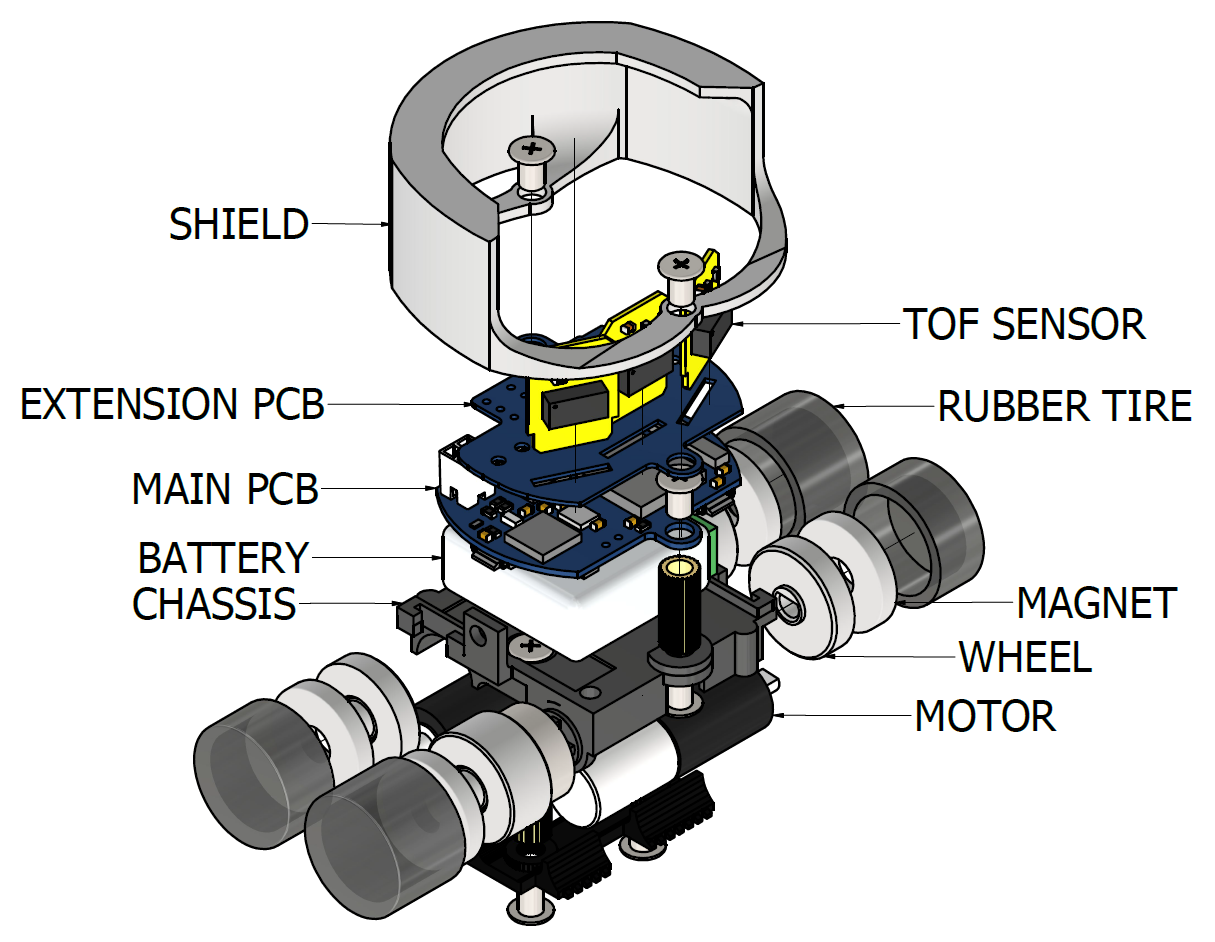
(b) 3D CAD view

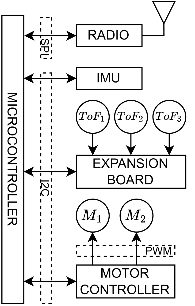
(c) Schematics view

Figure 2: We use a revised and extended version of the original Rovable robot [9]. (a) The extended robot with IR sensor board. (b) Exploded 3D CAD view of the extended robot. (c) Electronic block diagram of the extended robot. The micro-controller (Atmel SAMD21G18) interfaces with the IMU (MPU6050), 2.4 GHz radio (nRF24L01+), motor-controllers (DRV8835), and ToF IR sensors (VL53L1X).

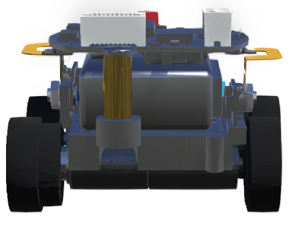
(a) Simulation, front

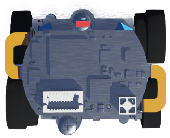
(b) Simulation, top

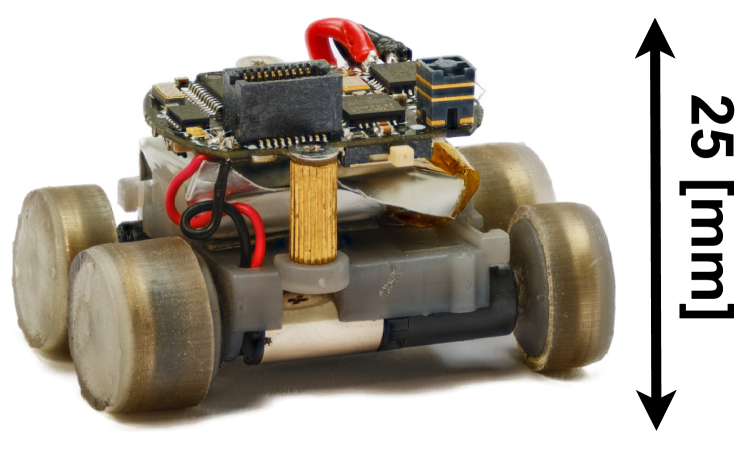
(c) Real robot, front

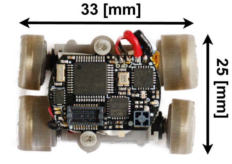
(d) Real robot, top

Figure 3: We use a simpler robot model in simulation, with IR sensors directly simulated on the main PCB. Simulated collision avoidance closely matches reality.

4 Simulation and Optimization Framework

Our simulation framework provides a virtual environment where we can study the operation of our robot swarm. The ease and speed of launching simulations enables optimization. Within Webots, we set up two main components: (i) a realistic model of our $3cm$ wheeled robot, and (ii) a tiled surface that the robots inspect, with a black and white projected floor pattern. We use the black and white tiles in simulation as a proxy for vibrating and non-vibrating tiles in our real experimental setup. In simulation, we assume noise-free binary sampling of the surface and zero loss on inter-robot communication. Figure 3 shows the simulated and the real robots side by side. In simulation, the ToF sensor board is absent, but simulated IR sensors retain comparable range and positioning. We recreate mechanical differences that exist between real robots by adding randomized offsets to the simulated left and right motor speed commands:

$$M_{l}^{s}\leftarrow M_{l}^{s}r_{v}(1-r_{a})$$ (1a)

$$M_{r}^{s}\leftarrow M_{r}^{s}r_{v}(1+r_{a})$$ (1b)

where $M_{l}^{s}$ and $M_{r}^{s}$ are the left and right motor speeds, and $r_{v}$ and $r_{a}$ are drawn from empirically chosen uniform distributions $U\sim(0.95,1.05)$ and $U\sim(-0.125,0.125)$, respectively, to account for variations in motor speed and alignment. We calibrate our simulation empirically considering three characteristic features: (i) sample distribution over the experimental setup, (ii) time between consecutive samples, and (iii) distance between consecutive samples. To obtain data for our calibrations, we run experiments using five robots for 3 $\times$ 20 minutes with algorithm parameters $[\gamma,\gamma_{0},\tau,\theta_{c}]=[5000,2000,1500,60]$ using the $u^{-}$ information sharing strategy (see Section 5). The Pearson correlation coefficients for the obtained data shown in Figure 4 corresponding to the three features mentioned above are calculated as $0.990$, $0.984$, and $0.735$, respectively. These values confirm the similarity between simulated and real swarm behaviors, enabling optimizing real experiments using simulation.

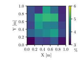
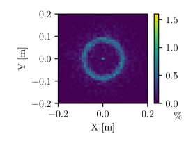
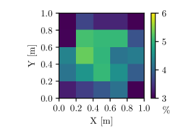
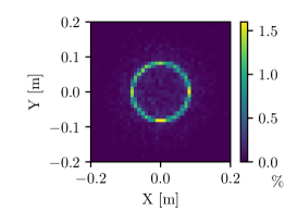
(a) (b) (c) (d)

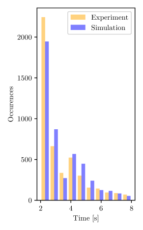
(e)

Figure 4: Distribution of samples across tiles in real (a) and simulated (c) setups. The displacement between consecutive samples in real (b) and simulated (d) setups. Time lapsed between consecutive samples in both setups is shown in (e).

Our optimization framework involves two components: (i) our calibrated simulation and (ii) a noise-resistant PSO method. Throughout the PSO iterations, every particle is evaluated multiple times on randomized floor patterns with the same fill-ratio. The velocity and position of particle $i$ are updated at iteration $k$ as:

$$\mathbf{v}_{i}^{k+1}=\omega\cdot\mathbf{v}_{i}^{k}+\omega_{p}\cdot\mathbf{r_{1}}(\mathbf{p}_{b_{i}}-\mathbf{p}_{i}^{k})+\omega_{g}\cdot\mathbf{r_{2}}(\mathbf{g}_{b}-\mathbf{p}_{i}^{k})$$ (2a)

$$\mathbf{p}_{i}^{k+1}=\mathbf{p}_{i}^{k}+\mathbf{v}_{i}^{k+1}$$ (2b)

where $\mathbf{v}_{i}^{k}$ and $\mathbf{p}_{i}^{k}$ are the velocity and position vector of particle $i$ at iteration $k$. $\mathbf{p}_{b_{i}}$ and $\mathbf{g}_{b}$ correspond to the position vector of the personal best and global best evaluations for particle $i$, respectively. We set the PSO weights for inertia, personal best, and global best as $[\omega\ \omega_{p}\ \omega_{g}]=[0.75\ 1.5\ 1.5]$, balancing local and global exploration [21, 13, 16]. The values $\mathbf{r_{1}}$ and $\mathbf{r_{2}}$ are drawn from a uniform distribution $U\sim(0,1)$ each iteration.

5 Inspection Algorithm

Algorithm 1 shows the collective Bayesian decision making algorithm that we study. The robots individually estimate and classify the fill ratio $f$ as above or below 0.5. Each robot acts as a Bayesian modeler integrating personal observations and information broadcast by other robots. The content of this shared information depends on the swarm’s information sharing strategy. We consider three strategies: (i) the no feedback ($u^{-}$) and (ii) the positive feedback ($u^{+}$) strategies, which were previously studied in [11], and (iii) the soft feedback ($u^{s}$) strategy, which we propose as a new approach.

The robots make binary observations of the surface condition as black/white in simulation or vibrating/non-vibrating in the real setup which we model as $O\in\{0,1\}$:

$$O\sim\textrm{Bernoulli}(f)$$ (3)

The fill ratio $f\in[0,1]$ is unknown to the robots and is modeled by a Beta-distribution:

$$f\sim\textrm{Beta}(\alpha,\beta)$$ (4)

The prior distribution of $f$ is initialized as $\text{Beta}(\alpha_{0}=1,\beta_{0}=1)$. Upon sampling or receiving observations from other robots, the posterior distribution of $f$ is updated as:

$$f\ |\ O\sim\textrm{Beta}(\alpha+O,\beta+(1-O))$$ (5)

Algorithm 1 Collective Bayesian Decision Making

Inputs:      $u^{-},u^{+},u^{s},T_{end},\theta_{o},\eta,\theta_{c},\tau,p_{c}$

Initialize:       $\alpha=1,\beta=1,d_{f}=-1,\text{robot }id,t_{s}=0$

while $t<T_{end}$ do

    Perform random walk for $\tau$ time

    if $t-t_{s}>\tau$ then

        $O\leftarrow$ Observation$\triangleright$ Get binary observation

        $t_{s}\leftarrow t$ $\triangleright$ Observation timestamp

        $\text{Beta}(\alpha,\beta)\leftarrow\textrm{Beta}(\alpha+O,\beta+(1-O))$ $\triangleright$ Update modeling of $f$

        $p\leftarrow P(\text{Beta}(\alpha,\beta)<0.5)$$\triangleright$ Update belief on $f$

        $O_{count}\leftarrow O_{count}+1$ $\triangleright$ Observation count

    end if

    if $(u^{s}\text{ {Or} }d_{f}==-1)$ And $(O_{count}>\theta_{o})$ then

        if $p>p_{c}$ then

           $d_{f}\leftarrow 0$

        else if $(1-p)>p_{c}$ then

           $d_{f}\leftarrow 1$

        end if

    end if

    if $u^{s}$ then

        $\Gamma\leftarrow\text{Var(Beta)}$

        $m\leftarrow\text{Bernoulli}\left((1-p)e^{-\eta\Gamma}(\frac{1}{2}-p)^{2}+O(1-e^{-\eta\Gamma}(\frac{1}{2}-p)^{2})\right)$

        Broadcast($m$) $\triangleright$ Soft feedback

    else if ($u^{+}$ And $d_{f}\neq-1$) then

        Broadcast($d_{f}$) $\triangleright$ Positive feedback

    else

        Broadcast($O$)$\triangleright$ No feedback

    end if

    if Message in queue then

        $O\leftarrow$ Message $\triangleright$ Receive message from swarm

        $\text{Beta}(\alpha,\beta)\leftarrow\textrm{Beta}(\alpha+O,\beta+(1-O))$ $\triangleright$ Update modeling of $f$

    end if

end while

The robots perform a Levy-flight type random walk, moving forward for a time drawn from a Cauchy distribution with mean $\gamma_{0}$ and average absolute deviation $\gamma$ followed by turning a uniform random angle $\phi\sim U(-\pi,\pi)$ in the direction of $\text{sign}(\phi)$ relative to the forward driving direction. The robots perform collision avoidance upon detecting an obstacle within a range of $\theta_{c}$ millimeters, by turning a random angle $\phi\sim U(-\pi,\pi)$ in the direction of $\text{sign}(\phi)$ relative to the forward driving direction.

Every $\tau$ milliseconds a robot samples a new observation $O$. In simulation, $O$ is based on a binary floor color sampling. In experiments, $O$ is calculated using a 500 millisecond vibration signal sample. The DC component of this sample is removed by employing a first-order high-pass filter with cutoff frequency $\omega_{n}=40$ Hz. Given a sampling rate of $350$ Hz, the filter parameters $\alpha_{1}$, $\alpha_{2}$, and $\alpha_{3}$ are configured to values: $0.20$, $0.60$, and $-0.60$ respectively. We define the filtered signal at time step $i$ as $\hat{a}_{i}$:

$$\hat{a}_{i}:=\alpha_{1}\hat{a}_{i-1}+\alpha_{2}a_{i}+\alpha_{3}a_{i-1}$$ (6)

where $a_{i}$ is the magnitude of the IMU’s raw acceleration data $a_{x}$, $a_{y}$, and $a_{z}$. The Root-Mean-Square (RMS) of $\hat{a}$ returns the energy of the signal as $\hat{E}=\sqrt{\frac{1}{n}\sum_{i=1}^{n}\hat{a}_{i}^{2}}$. Subsequently, the observation $O$ is determined by comparing $\hat{E}$ with a threshold $\theta_{E}$:

$$O=\begin{cases}1&\text{if }\hat{E}>\theta_{E}\\ 0&\text{if }\hat{E}\leq\theta_{E}\end{cases}\\$$ (7)

Depending on the information sharing strategy, the robots broadcast either (i) the latest observation $O$, in the case of no feedback ($u^{-}$), (ii) the latest observation $O$ before reaching a final decision, and after that their final decision $d_{f}$, in the case of positive feedback ($u^{+}$), or (iii) a binary value calculated through the soft-feedback method ($u^{s}$) as a Bernoulli sample with a probability determined by the soft feedback parameter $\eta\in\mathbb{R}^{+}$, the current observation $O\in\{0,1\}$, and the current belief $p\in[0,1]$ as below:

$$m\sim\text{Bernoulli}\left(\delta\cdot(1-p)+(1-\delta)\cdot O\right)$$ (8a)

$$\delta=e^{-\eta\Gamma}(\frac{1}{2}-p)^{2}$$ (8b)

$$p=P(\text{Beta}(\alpha,\beta)<0.5)$$ (8c)

where $m$ is the outgoing message, $\Gamma$ is the variance of the Beta distribution and $p$ is the robot’s belief evaluated as the CDF of the Beta distribution at $f=0.5$. Equation 8b depends on (i) a compelling component $e^{-\eta\Gamma}\in[0,1]$ which increases the proportion of the current belief in messages as $\Gamma$ decreases, and (ii) a stabilizing component $(\frac{1}{2}-p)^{2}\in[0,0.25]$ which is the squared distance of $p$ from the indecisive state $p=0.5$, increasing the proportion of robot’s belief in the Bernoulli sampled message to enhance accuracy.

Upon reaching a minimum of $\theta_{o}$ number of observations, a robot considers making a final decision based on its belief $p$. If above the credibility threshold $p_{c}$, the robot’s final decision $d_{f}$ is set to 0. Conversely, if $(1-p)>p_{c}$, this final decision is set to 1. The inspection task ends when all robots have made a final decision.

6 Experiments and Results

We use a swarm of five robots, all employing $p_{c}=0.95$, and floor patterns with a fill ratio of $f=0.48$ to conduct simulation and real experiments. We evaluate on decision time and accuracy for the strategies $u^{-}$, $u^{+}$, and $u^{s}$. We consider decision time as the time the last robot that makes a final decision. We average the beliefs (Equation 8c) of the robots at this decision time to calculate a corresponding decision accuracy.

6.1 Simulation Experiments

Parameter	$\gamma_{0}$[ms]	$\gamma$[ms]	$\tau$[ms]	$\theta_{c}$[mm]	$\theta_{o}$
$P_{0}$	2000	5000	2000	60	50
$\text{min}_{i}$	2000	0	1000	50	50
$\text{max}_{i}$	15000	15000	3000	100	200
$P^{*}$	7565	15000	2025	50	85

Table 1: The PSO optimization parameters and bounds. $P_{0}$ is the empirical best guess particle. $P^{*}$ is the resulting best particle with respect to our cost-function.

Five algorithmic parameters determine the sampling behavior of the swarm. These include mean ($\gamma_{0}$) and mean absolute deviation ($\gamma$) of the Cauchy distribution characterizing the robots’ random walk, the sampling interval ($\tau$), the collision avoidance threshold ($\theta_{c}$), and the observations threshold ($\theta_{o}$). Table 1 lists the boundaries of our optimization search space. The lower bounds for $\tau$ and $\theta_{c}$ are set to allow smooth pause-sample-move and collision avoidance maneuvers. The bounds on $\gamma$ and $\gamma_{0}$ are set such that a robot is able to cross the arena in one random walk step. The bounds on the observation threshold $\theta_{o}$ are established empirically. The particles in the PSO swarm are initialized randomly within the bounded search space, with the exception of one particle $P_{0}$ set to an empirically chosen location. Each particle is evaluated multiple times to mitigate randomness. For a particle $i$, we define the performance cost $\mathcal{C}_{i}$ as:

$$\mathcal{C}_{i}=\mu\left(\begin{bmatrix}c_{1}&c_{2}&\ldots&c_{N_{e}}\end{bmatrix}^{\top}\right)+1.1\cdot\sigma\left(\begin{bmatrix}c_{1}&c_{2}&\ldots&c_{N_{e}}\end{bmatrix}^{\top}\right)$$ (9)

where $N_{e}$ is the number of re-evaluations and $c_{j}$ is the outcome of the evaluation $j$:

$$\epsilon_{i}(t,d_{f})=\begin{cases}\epsilon_{f}\cdot t/T_{end}&d_{f}=d_{f}^{*}\\ \epsilon_{f}\cdot\epsilon_{d}&d_{f}\neq d_{f}^{*}\\ \epsilon_{f}&d_{f}=-1\end{cases}$$ (10a)

$$c_{j}=\sum_{i=1}^{N_{r}}\epsilon_{i}$$ (10b)

where $N_{r}=5$ is the number of robots, $\epsilon_{i}$ is the performance cost of robot $i$ for which the robot’s final decision $d_{f}$ made at time $t$ is compared with the correct decision $d_{f}^{*}$. A wrong decision is penalized by a factor of $\epsilon_{d}=5$. The value $\epsilon_{f}=1+|f-f^{*}|/\epsilon_{t}$ is calculated using the absolute difference between a robot’s current estimate of the fill ratio $f=\alpha/(\alpha+\beta)$ and the correct fill ratio $f^{*}$, divided by a normalizing factor $\epsilon_{t}=0.04$ that corresponds to the contribution of one tile in the overall 25-tile setup.

To find the optimal parameters for our inspection algorithm, we first consider running the algorithm with the $u^{-}$ information sharing strategy through our optimization framework. Our intuition is that an optimal parameter set for $u^{-}$ should allow the swarm to obtain a well-representative sample of the environment in a time-efficient manner, thus, the same parameters should also perform optimally for $u^{+}$ and $u^{s}$. Using this parameter set, we then run a systematic search to find an optimal value for the soft feedback parameter $\eta$ that characterizes the $u^{s}$ information sharing strategy.

We consider the $u^{-}$ strategy first. For the PSO optimizations, we use 30 particles, 50 iterations, and 16 re-evaluations. Each particle is evaluated for $T_{end}=1200s$ or until all robots in the swarm have reached a decision. The optimization results are shown in Figure 5. It can be seen that the average personal best performance of the particles converges to the performance of the global best particle $P^{*}$, which is listed in Table 1.

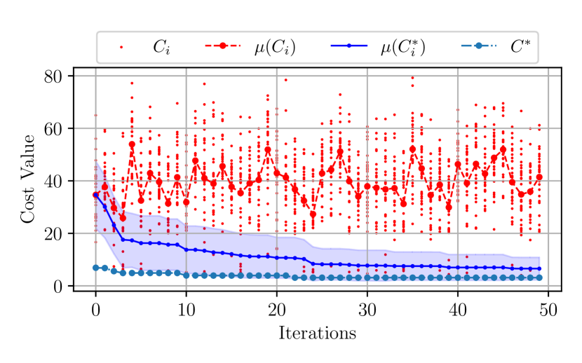
(a) Cost performance over iterations.

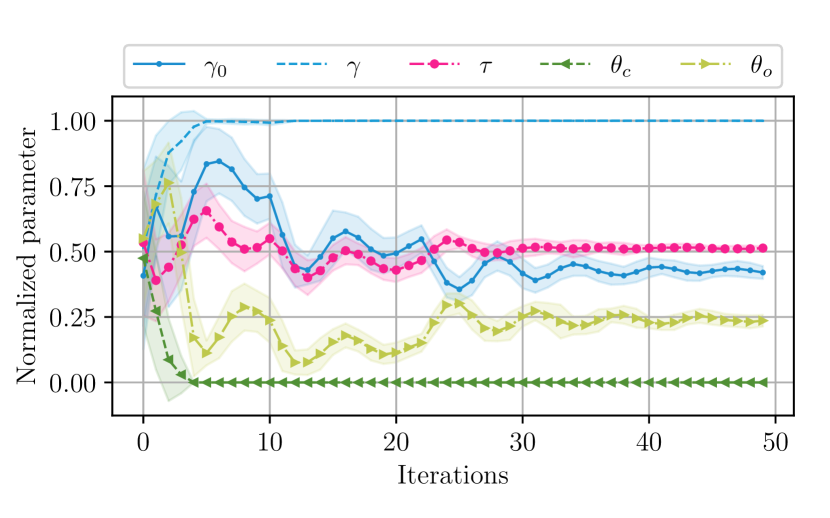
(b) Average values of particle parameters.

Figure 5: We use 30 particles, each re-evaluated 16 times, over 50 iterations using Equation 9. (a) Progression of cost performance of each particle ($C_{i}$), personal best cost performance of each particle ($C^{*}_{i}$), and the global best cost performance ($C^{*}$). (b) Progression of mean and standard deviation of parameters in Table 1.

Using $P^{*}$, we then run a systematic search for the soft-feedback parameter $\eta$. We consider five candidate values for $\eta$ based on prior empirical tests and run 100 randomized simulations to evaluate the performance of $u^{s}$ against $u^{-}$ and $u^{+}$. Figure 6 illustrates the results. We see that $u^{s}$ consistently outperforms $u^{-}$ and $u^{+}$ in decision time. Regarding accuracy, $u^{s}$ closely approaches the performance of $u^{+}$ and $u^{-}$ at $\eta=1000$. Specifically, for $\eta=1000$, the $u^{s}$ achieves a $20.52\%$ reduction in mean decision time at a $0.78\%$ loss in accuracy, compared with $u^{+}$. When compared with $u^{-}$, $u^{s}$ achieves a reduction of $22.10\%$ in mean decision time at a $1.22\%$ loss in accuracy.

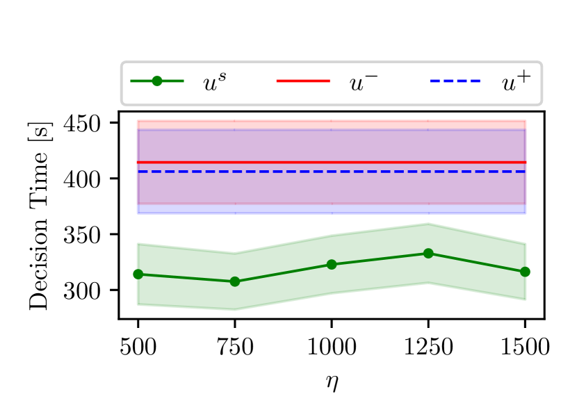
(a) Decision time for $\eta$ values.

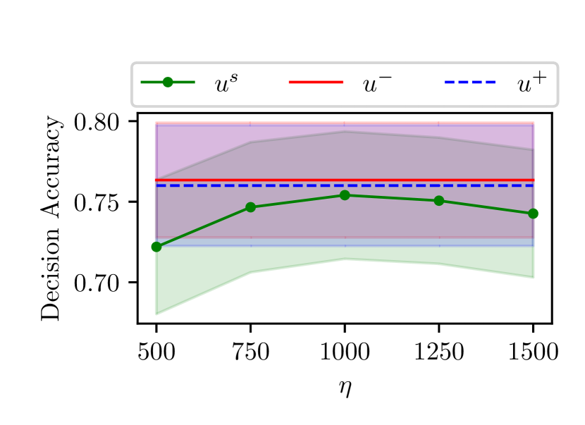
(b) Decision accuracy for $\eta$ values.

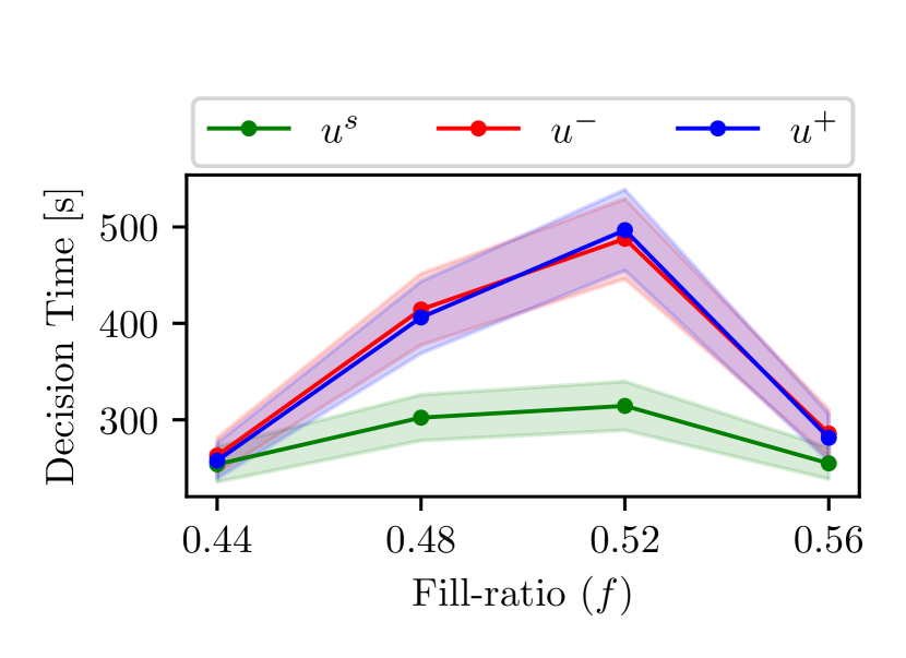
(c) Decision time for $f$ values.

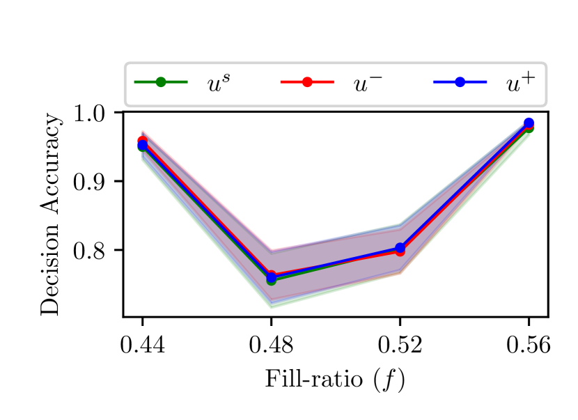
(d) Decision accuracy for $f$ values.

Figure 6: Decision time (a) and decision accuracy values (b) of 100 randomized simulation experiments using systematic search for the soft-feedback parameter $\eta$ of $u^{s}$, compared against $u^{-}$ and $u^{+}$. Using $\eta=1000$ we run 100 randomized simulations for different $f\in[0.44,0.48,0.52,0.56]$ and compare with $u^{-}$ and $u^{+}$. The resulting decision times and accuracies are shown in (c) and (d), respectively.

To assess the generalizability of our findings, we run 100 randomized simulations across fill-ratios of $f\in[0.44,0.48,0.52,0.56]$ to compare $u^{-}$, $u^{+}$ and $u^{s}$ (with $\eta=1000$) based on decision time and accuracy. Each simulation ends upon reaching $T_{end}$ or when all robots have reached a decision. For a fair comparison, we fix the random seeds used to generate floor patterns across the simulation instances. Figure 6c shows that $u^{s}$ outperforms the other two strategies in decision time. Due incorporating beliefs in the shared information, the swarm is compelled to make a decision rapidly, reducing mean and variation in decision times. This is particularly beneficial in harder environments where the fill ratio is close to $f=0.5$, facilitating reaching the credibility threshold $p_{c}$.

6.2 Real Experiments

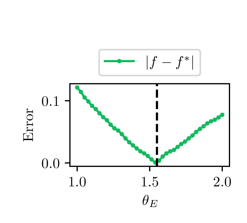
(a) $|f-f^{*}|$ vs $\theta_{E}$

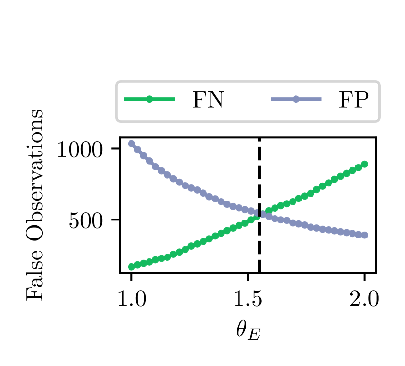
(b) FP and FN vs $\theta_{E}$

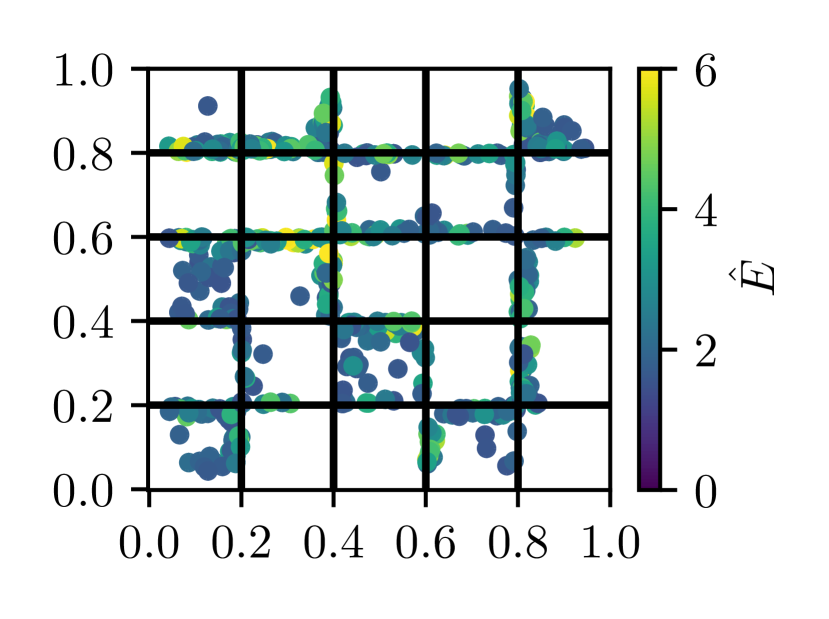
(c) FPs in arena

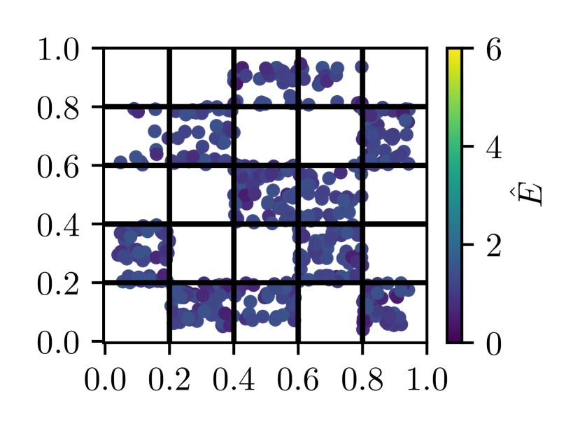
(d) FNs in arena

Figure 7: The threshold parameter $\theta_{E}$ determines binary observations of vibration data in real experiments (see Equation 7). (a) The fill ratio error $|f-f^{*}|$ for different values of $\theta_{E}$ (0.025 grid). (b) False observations for different values of $\theta_{E}$ (c) Spatial distribution of false positive and (d) false negative observations.

We validate our simulation results by real experiments in 10 trials for $u^{-},u^{+}$, and $u^{s}$. We first tune the sample threshold $\theta_{E}$ using data from one hour of swarm operation employing $u^{-}$ and algorithm parameters $[\gamma,\gamma_{0},\tau,\theta_{c}]=[5000,2000,1000,60]$, gathering a total of 6975 samples. Our evaluation criteria are the number of false observations and the fill-ratio error $|f-f^{*}|$. Figure 7 shows that we obtain $|f-f^{*}|\approx 0$ at $\theta_{E}=1.55$. Employing $\theta_{E}=1.55$ results in an equal amount of False Positives (FP) and False Negatives (FN), balancing the modeling error on the Beta distribution. Furthermore, we note that false observations appear mostly along edges of the tiles. This is expected as the robots may sample close to the tile edges while in contact with two tiles.

We conduct 10 experimental trials on our experimental setup with $f^{*}=0.48$ for assessing $u^{-}$, $u^{+}$ and $u^{s}$. The real experiments confirm our findings in simulation and reveal that the utilization of $u^{s}$ notably decreases the swarm’s decision time. Employing $u^{s}$ compels the swarm to reach decisions at an accelerated rate compared to $u^{+}$ and $u^{-}$. The decision time and accuracy data from real experiments is shown in Figure 8. We can see that $u^{s}$ demonstrates inherently less variance in decision times. Moreover, we encounter fewer indecisive trial outcomes compared to $u^{+}$ and $u^{-}$.

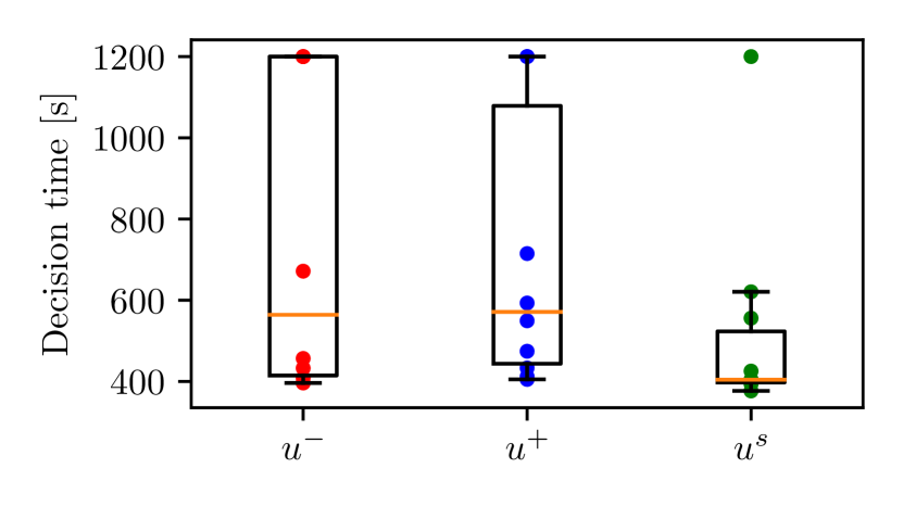
(a) Decision time

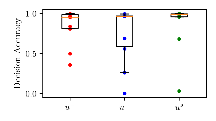
(b) Decision accuracy

Figure 8: Decision time and accuracy in real experiments with a fill-ratio of $f=0.48$. If no decision is made within $t=T_{end}$, we refer to $1200$ for decision time and the corresponding belief for accuracy. We see that $u^{s}$ is faster and equally accurate as $u^{-}$ and $u^{+}$ in real experiments, confirming our simulation results.

7 Conclusion and Future Work

In this work, we presented an experimental setup for studying a surface inspection task using a swarm of vibration sensing robots and explored the application of a Bayesian decision-making algorithm. We developed a simulation framework leveraging the physics based Webots robotic simulator and a PSO method to optimize the parameters shaping the robots’ sampling performance. The resulting optimal parameter values were assessed for three information sharing strategies in randomized simulations across different environments based on the swarm’s decision time and accuracy. We observed that our proposed soft feedback strategy yields a significant decrease in decision time without a major compromise in decision accuracy, compared to two previously studied strategies. Furthermore, hardware experimental trials validated our simulation findings. In real experiments, no drop in the decision accuracy was observed, demonstrating the adaptability and robustness of the decision-making processes to noise. In our future work, we plan to increase the complexity of our experiments in several ways, considering (i) performing inspection of complex structures such as 3D surfaces or obstacle-dense environments, (ii) classifying time-varying fill-ratios on our experimental setup, and (iii) studying the effect of the swarm size on the inspection performance.

References

- [1] Alanyali, M., Venkatesh, S., Savas, O., Aeron, S.: Distributed bayesian hypothesis testing in sensor networks. In: Proceedings of the American Control Conference. vol. 6, pp. 5369–5374. Institute of Electrical and Electronics Engineers Inc. (2004). https://doi.org/10.23919/acc.2004.1384706
- [2] Arnaud Deraemaeker, Keith Worden: New Trends in Vibration Based Structural Health Monitoring. Springer Vienna (2010)
- [3] Bayat, B., Crasta, N., Crespi, A., Pascoal, A.M., Ijspeert, A.: Environmental monitoring using autonomous vehicles: a survey of recent searching techniques (6 2017). https://doi.org/10.1016/j.copbio.2017.01.009
- [4] Bigoni, C., Zhang, Z., Hesthaven, J.S.: Systematic sensor placement for structural anomaly detection in the absence of damaged states. Computer Methods in Applied Mechanics and Engineering 371 (11 2020). https://doi.org/10.1016/j.cma.2020.113315
- [5] Bousdekis, A., Apostolou, D., Mentzas, G.: Predictive Maintenance in the 4th Industrial Revolution: Benefits, Business Opportunities, and Managerial Implications. IEEE Engineering Management Review 48(1), 57–62 (1 2020). https://doi.org/10.1109/EMR.2019.2958037
- [6] Brem, C., Siemens: Senseye Predictive Maintenance - Whitepaper True Cost Of Downtime 2022 (2023)
- [7] Carbone, C., Garibaldi, O., Kurt, Z.: Swarm Robotics as a Solution to Crops Inspection for Precision Agriculture. KnE Engineering 3(1), 552 (2 2018). https://doi.org/10.18502/keg.v3i1.1459
- [8] Chiu, D., Nagpal, R., Haghighat, B.: Optimization and Evaluation of Multi Robot Surface Inspection Through Particle Swarm Optimization (10 2023), http://arxiv.org/abs/2310.03172
- [9] Dementyev, A., Kao, H.L.C., Choi, I., Ajilo, D., Xu, M., Paradiso, J.A., Schmandt, C., Follmer, S.: Rovables: Miniature on-body robots as mobile wearables. In: UIST 2016 - Proceedings of the 29th Annual Symposium on User Interface Software and Technology. pp. 111–120. Association for Computing Machinery, Inc (10 2016). https://doi.org/10.1145/2984511.2984531
- [10] Doebling, S., Farrar, C., Prime, M., Shevitz, D.: Damage identification and health monitoring of structural and mechanical systems from changes in their vibration characteristics: A literature review. Tech. rep. (1996)
- [11] Ebert, J.T., Gauci, M., Mallmann-Trenn, F., Nagpal, R.: Bayes Bots: Collective Bayesian Decision-Making in Decentralized Robot Swarms. In: ICRA (2020). https://doi.org/10.1109/ICRA40945.2020.9196584
- [12] Ebert, J.T., Gauci, M., Nagpal, R.: Multi-Feature Col-lective Decision Making in Robot Swarms. In: Proc. ofthe 17th International Conference on Autonomous Agents and Multiagent Systems (AAMAS). vol. 9 (2018)
- [13] Gad, A.G.: Particle Swarm Optimization Algorithm and Its Applications: A Systematic Review. Archives of Computational Methods in Engineering 29(5), 2531–2561 (8 2022). https://doi.org/10.1007/s11831-021-09694-4
- [14] Haghighat, B., Ebert, J., Boghaert, J., Ekblaw, A., Nagpal, R.: A Swarm Robotic Approach to Inspection of 2.5 D Surfaces in Orbit (2022)
- [15] Halder, S., Afsari, K.: Robots in Inspection and Monitoring of Buildings and Infrastructure: A Systematic Review (2 2023). https://doi.org/10.3390/app13042304
- [16] Innocente, M.S., Sienz, J.: Coefficients’ Settings in Particle Swarm Optimization: Insight and Guidelines. Mecánica Computacional: Computational Intelligence Techniques for Optimization and Data Modeling XXIX, 9253–9269 (2010)
- [17] Lee, A.J., Song, W., Yu, B., Choi, D., Tirtawardhana, C., Myung, H.: Survey of robotics technologies for civil infrastructure inspection. Journal of Infrastructure Intelligence and Resilience 2(1), 100018 (3 2023). https://doi.org/10.1016/j.iintel.2022.100018
- [18] Liu, Y., Hajj, M., Bao, Y.: Review of robot-based damage assessment for offshore wind turbines (4 2022). https://doi.org/10.1016/j.rser.2022.112187
- [19] Magalhães, F., Cunha, A., Caetano, E.: Vibration based structural health monitoring of an arch bridge: From automated OMA to damage detection. Mechanical Systems and Signal Processing 28, 212–228 (4 2012). https://doi.org/10.1016/j.ymssp.2011.06.011
- [20] Makarenko, A., Durrant-Whyte, H.: Decentralized Bayesian algorithms for active sensor networks. Information Fusion 7(4 SPEC. ISS.), 418–433 (2006). https://doi.org/10.1016/j.inffus.2005.09.010
- [21] Poli, R., Kennedy, J., Blackwell, T.: Particle swarm optimization. Swarm Intelligence 1(1), 33–57 (10 2007). https://doi.org/10.1007/s11721-007-0002-0
- [22] PwC: PdM 4.0. Tech. rep. (2017)
- [23] Roda, I., Macchi, M., Fumagalli, L.: The future of maintenance within industry 4.0: An empirical research in manufacturing. In: IFIP Advances in Information and Communication Technology. vol. 536, pp. 39–46. Springer New York LLC (2018). https://doi.org/10.1007/978-3-319-99707-0_6
- [24] Schranz, M., Umlauft, M., Sende, M., Elmenreich, W.: Swarm Robotic Behaviors and Current Applications (4 2020). https://doi.org/10.3389/frobt.2020.00036
- [25] Seeley, T.D., Buhrman, S.C.: Group decision making in swarms of honey bees. Behav Ecol Sociobiol 45, 19–31 (1999)
- [26] Valentini, G., Brambilla, D., Hamann, H., Dorigo, M.: Collective Perception of Environmental Features in a Robot Swarm 9882 (2016). https://doi.org/10.1007/978-3-319-44427-7
- [27] Valentini, G., Ferrante, E., Hamann, H., Dorigo, M.: Collective decision with 100 Kilobots: speed versus accuracy in binary discrimination problems Collective decision with 100 Kilo-bots: speed versus accuracy in binary discrimination problems. Autonomous Agents and Multi-Agent Systems 30(3), 553–580 (2016). https://doi.org/10.1007/s10458-015-9323-3