High-fidelity Nuclear Coherent Population Transfer via the Mixed-State Inverse Engineering

Abstract

Nuclear coherent population transfer (NCPT) plays an important role in the exploration and application of atomic nuclei. How to achieve high-fidelity NCPT remains so far challenging. Here, we investigate the complete population transfer of nuclear states. We first consider a cyclic three-level system, based on the mixed-state inverse engineering scheme by adding additional laser fields in an open three-level nuclear system with spontaneous emission. We find the amplitude of the additional field is related to the ratio of the pump and Stokes field amplitudes. As long as an appropriate additional field is selected, complete transfer can be achieved even when the intensities of the pump and Stokes fields are exceedingly low. The transfer efficiency exhibits excellent robustness with respect to laser peak intensity and pulse delay. We demonstrate the effectiveness through examples such as ²²⁹Th, ²²³Ra, ¹¹³Cd, and ⁹⁷Tc, which have a long lifetime excited state, as well as ¹⁸⁷Re, ¹⁷²Yb, ¹⁶⁸Er and ¹⁵⁴Gd with a short lifetime excited state. Focusing on the case without additional coupling, we further reduce the three-level system to an effective two-level problem. We modify the pump and Stokes pulses by using counterdiabatic driving to implement high-fidelity population transfer. The schemes open up new possibilities for controlling nuclear states.

I Introduction

Nuclear coherent population transfer (NCPT) holds significant importance across various areas, ranging from nuclear physics Di Piazza et al. (2012), quantum information processing Leskowitz and Mueller (2004); Leuenberger et al. (2002) and quantum computing Stetcu et al. (2022); Zhang et al. (2021a); Yeter-Aydeniz et al. (2020); Vandersypen and Chuang (2005); Roggero et al. (2020). Typically, NCPT can be used in studying nucleus, constructing nuclear batteries Aprahamian and Sun (2005); Carroll (2004); Belic et al. (1999); Walker and Dracoulis (1999); Pálffy et al. (2007); Walker et al. (2001), and creating nuclear clocks that exhibit considerably greater precision than atomic clocks Peik et al. (2021); Seiferle et al. (2019); Kazakov et al. (2012); Beeks et al. (2021); Campbell et al. (2012). Encouraged by the development of the X-ray free electron laser (XFEL) Feldhaus et al. (1997); Saldin et al. (2001); Wootton et al. (2002); Huang et al. (2021); Pellegrini et al. (2016); Altarelli (2011), the domain of the interaction of laser fields with nuclei has gained extensive attention Wong et al. (2011); Bürvenich et al. (2006a); Liao and Pálffy (2014); Gunst et al. (2015); Junker et al. (2012); von der Wense et al. (2020); Pálffy et al. (2015); Di Piazza et al. (2007). The combination of high-frequency laser facilities with moderate acceleration of target nuclei matches photon and transition frequency Bürvenich et al. (2006b). This allows for the active NCPT using coherent hard X-ray photons Liao (2014); Amiri and Niari (2023); Chen et al. (2022); Pálffy et al. (2011).

The stimulated Raman adiabatic passage (STIRAP) technique and its extensions are employed to transfer the population of states in different nuclear systems, including $\Lambda$-like three state system Liao et al. (2013); Nedaee-Shakarab et al. (2016); Liao et al. (2011); Kirschbaum et al. (2022); Mansourzadeh-Ashkani et al. (2021a), tripod system Nedaee-Shakarab et al. (2017), multi-lambda system Mansourzadeh-Ashkani et al. (2021b) and chain system Amiri and Saadati-Niari (2023). It offers a crucial benefit that the excited state is not populated during time evolution Bergmann et al. (1998). Moreover, it is also insensitive to variations of the pulse amplitude and time delay between pulses Bergmann et al. (2019). Provided sufficient X-ray intensity, STIRAP allows us to achieve NCPT, but may present challenges in practical experiments. Nowadays, the efficient manipulation of nuclear state populations remains an area yet to be deeply explored, with an ongoing pursuit of a method that can simultaneously achieve high-fidelity, exceptional controllability, and fast execution. Recently, a fast control method called the mixed-state inverse engineering (MIE) has been proposed Wu et al. (2021). The MIE scheme has been successfully applied to a single nitrogen-vacancy center and open two-level quantum systems Wang et al. (2024). In addition, on one-photon resonance, the three-level system can be reduced to an equivalent two-level model Vitanov and Stenholm (1997); Zhang et al. (2021b). Then a feasible shortcut scheme is designed via counterdiabatic driving along with unitary transformation Li and Chen (2016). By modifying only the pump and Stokes pulses, complete transfer can be achieved without introducing additional couplings. The question then arises as to how these schemes perform in nuclear systems?

In this work, we investigate the complete population transfer based on the MIE and feasible effective two-level shortcut schemes. We consider the nuclear $\Lambda$-scheme comprising the ground state $|1\rangle$, isomeric state $|2\rangle$ and excited state $|3\rangle$, as illustrated in Fig. 1. Three X-ray laser pulses are employed to control the atomic nucleus. The pump laser drives the transition $|1\rangle\to|3\rangle$ and Stokes laser drives the transition $|2\rangle\to|3\rangle$, respectively. The additional field couples states $|1\rangle$ and $|2\rangle$. We first calculate the complete population transfer in the nuclear system based on the MIE scheme and compare it with the traditional STIRAP protocol. Moreover, the effects of laser field strength and time delay on the transfer efficiency are simulated. We further analyse the benefits of MIE by calculating fidelity. Under one-photon resonance, we reduce the quantum three-level system to an effective two-level problem. By applying counterdiabatic driving together with the unitary transformation, the shapes of the pump and Stokes fields are modified to achieve high-fidelity population transfer.

The rest of this paper is organized as follows. In section II, we introduce the model and the MIE scheme. In section III, we investigate the complete population transfer in the nuclear system. The performance of MIE scheme is evaluated by analyzing the fidelity and robustness to parameter fluctuations. Then we focus on the case without additional coupling and discuss a feasible implementation based on the counterdiabatic driving of an effective two-level system to achieve high-fidelity population transfer. Finally, a briefly summary is given in section IV.

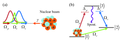
Figure 1: (a) Interaction between an accelerated nuclei and X-ray laser pulses in the laboratory frame. (b) The nuclear $\Lambda$-scheme. The initial population is in the state $|1\rangle$. The excited state $|3\rangle$ decays to other states through spontaneous emission. $\Omega_{p}$, $\Omega_{s}$ and $\Omega_{c}$ are the pump, Stokes and additional field laser pulses, respectively. $\gamma$ is the relativistic factor. $\Delta_{p}$ and $\Delta_{s}$ denote the detunings of the corresponding lasers.

II MODEL AND METHOD

We consider the system depicted in Fig. 1(a), which is composed of an accelerated nuclear beam that interacts with three incoming XFEL pulses. Here, the states $|1\rangle$ and $|3\rangle$ are coupled by pump laser pulse with Rabi frequency $\Omega_{p}(t)$ (red arrow), while states $|2\rangle$ and $|3\rangle$ are coupled by Stokes laser pulse with Rabi frequency $\Omega_{s}(t)$ (blue arrow). The additional field $\Omega_{c}(t)$ (green arrow) coupling states $|1\rangle$ and $|2\rangle$ is calculated by the MIE scheme. The interaction between the nucleus and lasers is also elucidated by a sketch like Fig. 1(b). The purple curve represents the spontaneous emission of the excited state. We model the population of this system with the density-matrix approach. The density matrix $\rho(t)$ is defined as Kirschbaum et al. (2022); Scully and Zubairy (1997)

$$\rho(t)=\sum_{i,j}\rho_{ij}(t)|i\rangle\langle j|,$$ (1)

where $\{i,j\}\in\{1,2,3\}$. The diagonal elements $\rho_{ii}$ represent the level population, while the off-diagonal elements $\rho_{ij}$ represent the coherences. The nuclear dynamics is governed by the master equation for the density matrix $\rho(t)$ Nedaee-Shakarab et al. (2016); Liao et al. (2013, 2011)

$$\frac{\partial}{\partial t}\rho(t)=\frac{1}{i\hbar}[H_{0}(t),\rho(t)]+\rho_{s}(t)+\rho_{d}(t),$$ (2)

where $\hbar$ represents the reduced Planck constant. The Hamiltonian $H_{0}(t)$ reads

$$H_{0}(t)=-\frac{\hbar}{2}\begin{pmatrix}0&0&\Omega_{p}(t)\\ 0&-2(\Delta_{p}-\Delta_{s})&\Omega_{s}(t)\\ \Omega_{p}(t)&\Omega_{s}(t)&2\Delta_{p}\end{pmatrix}.$$ (3)

Here, $\Delta_{p(s)}$ denotes the laser detuning. For simplicity, we assume the establishment of the full resonance condition $\Delta_{p(s)}=0$ in both theoretical and numerical calculations. $\rho_{s}(t)$ is the decoherence matrix induced by the spontaneous emission and has the following form

$$\rho_{s}(t)=\frac{\Gamma}{2}\left(\begin{array}[]{l l l}{{2B_{31}\rho_{33}}}&{{0}}&{{-\rho_{13}}}\\ {{0}}&{{2B_{32}\rho_{33}}}&{{-\rho_{23}}}\\ {{-\rho_{31}}}&{{-\rho_{32}}}&{{-2\rho_{33}}}\end{array}\right).$$ (7)

$\Gamma$ is the linewidth of the excited state $|3\rangle$, and $B_{3i}$ is the branching ratio of the transition $|3\rangle\to|i\rangle$, (i=1,2). $\rho_{d}(t)$ represents an additional dephasing matrix designed to model laser field pulses with limited coherence times. Consider a fully coherent XFEL source for both pump and Stokes lasers, then $\rho_{d}(t)$ is set to zero Nedaee-Shakarab et al. (2016). The slowly varying effective Rabi frequencies of laser pulses are given by Nedaee-Shakarab et al. (2016); Bergmann et al. (1998); Liao et al. (2013)

$$\begin{split}\Omega_{p(s)}(t)&=\Omega_{p0(s0)}\sqrt{I_{p(s)}}\exp\left\{-\left[\frac{\gamma(1+\beta)(t-\tau_{p(s)})}{\sqrt{2}T_{p(s)}}\right]^{2}\right\},\end{split}$$ (8)

with

$$\begin{split}\Omega_{p0(s0)}&=\sqrt{\frac{\gamma^{2}(1+\beta^{2})(L_{ij}+1)(2I_{i}+1)\mathbb{B}_{ij}(\mu L_{ij})}{c\varepsilon_{0}L_{ij}}}\\ &\times\frac{4\sqrt{\pi}k_{ij}^{L_{ij}-1}}{\hbar(2L_{ij}+1)!!}.\end{split}$$ (9)

The relativistic factor $\gamma=1/\sqrt{(1-\beta^{2})}$, where $\beta=v/c$ and $c$ is the velocity of light in vacuum. $\varepsilon_{0}$ is the vacuum permittivity. $L_{ij}$ is the multipolarity. $I_{i}$ is the nuclear spin of the level $|i\rangle$. $\mathbb{B}_{ij}(\mu L_{ij})$ is the reduced transition probability of the transition Pálffy et al. (2008). The index $\mu$ corresponds to the type of radiation multipole, either electric or magnetic, denoted by $\mu\in\left\{E,M\right\}$. $k_{ij}$ is the wave number. $I_{p(s)}$, $\tau_{p(s)}$ and $T_{p(s)}$ are the effective peak intensity, temporal peak position and pulse duration of pump (Stokes) laser, respectively.

Taking into consideration the radioactive decays of the excited state $|3\rangle$, we must establish adiabatic shortcuts in the open system. Firstly, extract the rows of the density matrix $\rho(t)$ and stack them one below the previous one, transforming the matrix into a $3^{2}$-dimensional coherence vector $|\rho\rangle\rangle$ as follows

$$|\rho(t)\rangle\rangle=(\rho_{11},\rho_{12},\rho_{13},\rho_{21},\rho_{22},\rho_{23},\rho_{31},\rho_{32},\rho_{33})^{T}.$$ (10)

Rewrite Eq. (2) via the coherent vector $|\rho\rangle\rangle$ is

$$\frac{\partial|\rho(t)\rangle\rangle}{\partial t}=\hat{\mathcal{L}}(t)|\rho(t)\rangle\rangle.$$ (11)

The Lindblad superoperator $\hat{\mathcal{L}}(t)$ becomes a $9\times 9$-dimensional supermatrix. The double brackets indicate that the state vectors are not in standard Hilbert space.

The MIE scheme enables robust and precise transitions to defined target states via a customisable mixed-state trajectory Wu et al. (2021, 2019); Lu et al. (2013). Here, select the instantaneous steady state $\rho_{\tau}(t)$ as the evolutionary trajectories. By solving $\hat{\mathcal{L}}(t)|\rho_{\tau}(t)\rangle\rangle=0$, we can get the trajectories

(12)

Then, the dynamical invariant of the open quantum system in the MIE scheme is defined $\hat{\mathcal{I}}(t)$ as Venuti et al. (2016); Sarandy et al. (2007)

$$\hat{\mathcal{I}}(t)=\Omega_{I}|\rho_{\tau}(t)\rangle\rangle\langle\langle I|,$$ (13)

where $\Omega_{I}$ is an arbitrary nonzero constant and $\langle\langle I|$ is the left vector corresponding to a $3\times 3$ identity matrix. Assume that the control Liouvillian is $\hat{\mathcal{L}}_{c}$

$$\frac{\partial}{\partial t}\rho(t) = \hat{\mathcal{L}}_{c}(t)\rho(t),$$ (14)

the control Liouvillian has the same form as Eq. (2),

$$\hat{\mathcal{L}}_{c}(t)\rho(t)=\frac{1}{i\hbar}[H_{c}(t),\rho(t)]+\rho_{s}{{}^{\prime}}(t),$$ (15)

with $H_{c}(t)$ is the control Hamiltonian

$$H_{c}(t)=-\frac{\hbar}{2}\begin{pmatrix}0&i\Omega_{c}(t)&\Omega_{p}{{}^{\prime}}(t)\\ -i\Omega_{c}(t)&0&\Omega_{s}{{}^{\prime}}(t)\\ \Omega_{p}{{}^{\prime}}(t)&\Omega_{s}{{}^{\prime}}(t)&0\end{pmatrix},$$ (16)

$\Omega_{p}{{}^{\prime}}(t)$, $\Omega_{s}{{}^{\prime}}(t)$ and $\Omega_{c}(t)$ are the control fields. The control decoherence matrix $\rho_{s}{{}^{\prime}}(t)$ is

$$\rho_{s}{{}^{\prime}}(t)=\frac{\Gamma{{}^{\prime}}}{2}\begin{pmatrix}2B_{31}{{}^{\prime}}\rho_{33}&0&-\rho_{13}\\ 0&2B_{32}{{}^{\prime}}\rho_{33}&-\rho_{23}\\ -\rho_{31}&-\rho_{32}&-2\rho_{33}\end{pmatrix},$$ (17)

$\Gamma{{}^{\prime}}$ denote the linewidth of the state $|3\rangle$ and $B_{3i}{{}^{\prime}}$ is the control branching ratio of the transition $|3\rangle\to|i\rangle$, where $i=1,2$. The dynamical invariant $\hat{\mathcal{I}}(t)$ and the control Liouvillian $\hat{\mathcal{L}}_{c}(t)$ satisfy

$$\frac{\partial\hat{\mathcal{I}}(t)}{\partial t}-[\hat{\mathcal{L}}_{c}(t),\hat{\mathcal{I}}(t)]=0.$$ (18)

In general, we need to parameterize the steady state $|\rho_{\tau}\rangle\rangle$ and the dynamical invariant $\hat{\mathcal{I}}(t)$ via the generalized Bloch vector $\{r_{i}\}_{i=1}^{8}$ Wu et al. (2021). Our aim is to evolve the system from an initial Liouvillian $\hat{\mathcal{L}}_{c}(0)$ to a final one, $\hat{\mathcal{L}}_{c}(t_{f})$. We set $[\hat{\mathcal{I}}(0),\hat{\mathcal{L}}_{c}(0)]=0$, $[\hat{\mathcal{I}}{(t_{f})},\hat{\mathcal{L}}_{c}(t_{f})]=0$, such that the transfer of the quantum state from the initial to the final state is guaranteed. More details can be found in Appendix A. Substituting Liouvillian $\hat{\mathcal{L}_{c}}(t)$ and Eq. (13) into Eq. (18), we can determine all the parameters in the control Liouvillian. Taking Eq. (8) and the Bloch vector into the analytical expressions, we can obtain the control parameters for the adiabatic trajectory

$$\Omega_{p}{{}^{\prime}}(t)= \Omega_{p}(t),\Omega_{s}{{}^{\prime}}(t)=\Omega_{s}(t),\rho_{s}{{}^{\prime}}(t)=\rho_{s}(t),$$

$$\begin{split}\Omega_{c}(t)&=2\dot{\theta}\\ &=\frac{4T_{p}^{2}\left(t-\tau_{s}\right)-4T_{s}^{2}\left(t-\tau_{p}\right)}{T_{p}^{2}T_{s}^{2}}\times\\ \end{split}$$ (19)

$$\frac{\exp\left\{-\frac{T_{s}^{2}\left(t-\tau_{p}\right)^{2}+T_{p}^{2}\left(t-\tau_{s}\right)^{2}}{T_{p}^{2}T_{s}^{2}}\right\}}{\alpha\exp\left\{-2\left[\frac{\left(t-\tau_{p}\right)}{T_{p}}\right]^{2}\right\}+\frac{1}{\alpha}\exp\left\{-2\left[\frac{\left(t-\tau_{s}\right)}{T_{s}}\right]^{2}\right\}},$$

where $\tan\theta(t)=\Omega_{p}(t)/\Omega_{s}(t)$ and $\alpha=\Omega_{s0}\sqrt{I_{s}}/\Omega_{p0}\sqrt{I_{p}}$.

III HIGH-FIDELITY NUCLEAR COHERENT POPULATION TRANSFER

The XLEF currently has two methods to improve the coherence of XFEL pulses, the XFEL oscillator (XFELO) Kim et al. (2008); Lindberg et al. (2011) and the seeded XFEL (SXFEL) Feldhaus et al. (1997). In our calculations, the SXFEL is selected with the laser photon energy of $12.4$ keV, the laser bandwidth of $10$ meV and the laser pulse duration of $0.1$ ps. The characteristic parameters of the nuclei used in our calculations are given in Appendix B. The arguments $E_{i}(i=1,2,3)$ represents the energy of states and $\hbar\omega_{p}$ is the energy of pump photon. Filling the energy gap based on the Doppler effect, the relativistic factor is given by the following condition $E_{3}-E_{1}=\gamma(1+\beta)\hbar\omega_{p}$. The time required for population transfer varies between nuclei, and this discrepancy arises from the fact that the width of the pulses in the nuclear frame depends on the distinct $\gamma$ parameter. The choice of laser frequency and the relativistic factor $\gamma$ for the accelerated nuclei must satisfy the requirement of exact resonance Bürvenich et al. (2006b).

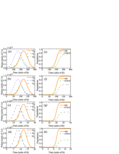
Figure 2: NCPT of the long lifetime excited state nuclei. (a)-(d) Pulse shapes for MIE and (e)-(h) populations as a function of time for ²²⁹Th, ²²³Ra, ¹¹³Cd and ⁹⁷Tc, respectively.

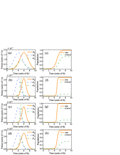
Figure 3: NCPT of the short lifetime excited state nuclei. (a)-(d) Pulse shapes for MIE and (e)-(h) populations as a function of time for ¹⁸⁷Re, ¹⁷²Yb, ¹⁶⁸Er and ¹⁵⁴Gd, respectively.

We calculate the time evolution of the target state population for the different nuclei using the MIE and STIRAP methods. The initial population is concentrated in state $|1\rangle$. Firstly, we consider long lifetime excited state nuclei for ²²⁹Th, ²²³Ra, ¹¹³Cd and ⁹⁷Tc, with lifetimes of 0.172 ns, 0.6 ns, 0.322 ns, and 0.76 ps, respectively. As the pulses presented in Figs. 2 (a)-(d) and the dynamic behavior controlled by the STIRAP and MIE schemes are shown in Figs. 2 (e)-(h). The orange solid line and green dotted line represent the populations of the target state for MIE and STIRAP methods. Compared to STIRAP, the MIE scheme can achieve nearly perfect NCPT. An important reason for this situation is that efficient transfer requires the STIRAP must meet adiabatic conditions. This typically requires a long time to evolve the system, and therefore the system has a long time to interact with the environment leading to decoherence or losses Blekos et al. (2020). For the MIE scheme, the state $|3\rangle$ remains unoccupied, effectively avoiding the decoherence during the transfer process. As shown in Fig. 3, we calculate nuclei with excited state lifetime shorter or slightly longer than the interaction time, including ¹⁸⁷Re, ¹⁷²Yb, ¹⁶⁸Er and ¹⁵⁴Gd with lifetimes of 54 fs, 11 fs, 3.5 fs and 1.54 fs respectively. Since the large energy gap between the energy levels of ¹⁷²Yb and ¹⁶⁸Er, a narrower bandwidth is required for the additional field. One of the significant advantages of the MIE scheme is that high-fidelity population transfer can be achieved regardless of whether the excited state lifetime of the nucleus exceeds the duration of the laser pulse.

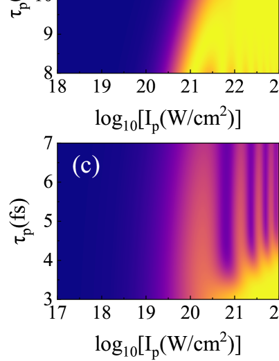
Figure 4: Contour plot of the final population of state $|2\rangle$ as a function of $I_{p}$ and $\tau_{p}$. For ⁹⁷Tc, in (a) the STIRAP and (b) the MIE scheme. The Stokes peak position $\tau_{s}$ is fixed at 6 fs. The Stokes laser intensity $I_{s}=23.514I_{p}$. For ¹⁶⁸Er, in (c) the STIRAP and (d) the MIE scheme. The Stokes peak position $\tau_{s}$ is fixed at 2 fs. The Stokes laser intensity $I_{s}=0.0703I_{p}$.

We further characterize the performance of the STIRAP and MIE methods through a meticulous analysis of the interdependence between the pump peak intensity $I_{p}$ and the temporal peak position of the laser $\tau_{p}$. We choose ⁹⁷Tc and ¹⁶⁸Er as examples. The results of the STIRAP are illustrated in Figs. 4 (a) and (c). The transfer efficiency is near 100$\%$ where the adiabatic condition is fully satisfied Bergmann et al. (1998). The dependence of transfer efficiency on parameter fluctuation can be qualitatively understood as follows: the dark state fails to adiabatically follow the STIRAP pulse, leading to reduced transfer efficiency. In contrast, as illustrated in Figs. 4 (b) and (d), the fidelity of the population transfer for the MIE method is robust against variations in both $I_{p}$ and $\tau_{p}$. The population is completely transferred from state $|1\rangle$ to state $|2\rangle$ without populating the middle state, even when the amplitudes of the pump and Stokes fields are very small.

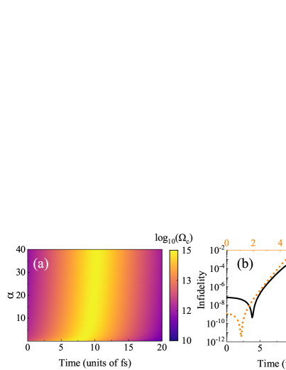
Figure 5: (a) Contour plot of the amplitude of the additional field as a function of $t$ and $\alpha$. Parameters: $\tau_{p}=12$ fs, $\tau_{s}=8$ fs, $T_{p}=T_{s}=100$ fs. (b) Infidelity as a function of time in the MIE scheme for ⁹⁷Tc (black solid line) and ¹⁵⁴Gd (orange dashed line).

To clearly analyse the benefits of the MIE scheme, we calculate the dependence of the additional field amplitude on the pump and Stokes field amplitudes based on Eq. (19). As shown in Fig. 5 (a), we can see more clearly that the intensity of the additional field is closely correlated with the ratio of the amplitudes of the pump and Stokes fields. As a result, pump and Stokes fields with lower field strengths always receive additional fields of corresponding strength (10¹⁵ W/cm²), controlling perfect population transfer. To further characterize the effectiveness of MIE, the fidelity $\mathcal{F}(t)$ is defined by

$$\mathcal{F}(t)=\left[\mathrm{tr}\left(\sqrt{\sqrt{\rho(t)}\rho_{\tau}\sqrt{\rho(t)}}\right)\right]^{2}.$$ (20)

which measures the distance between the target state $\rho(\tau)=\rho_{\tau}$ and the time evolved state $\rho(t)$ Taddei et al. (2013); Caneva et al. (2009). The infidelity $1-\mathcal{F}(t)$ of ⁹⁷Tc and ¹⁵⁴Gd is shown in Fig. 5 (b). For both long and short lifetime excited state nuclei, the infidelity can be kept below 10^-2. The system evolves completely along the instantaneous steady state. These results demonstrate that the MIE scheme exhibits excellent performance in NCPT and provides new ideas for the coherent control of nuclear states.

We further consider the case where there is no additional coupling to the initial and final states, which may be easily reached experimentally. On one-photon resonance ($\Delta=0$), we simplify the three-level system to an equivalent two-level problem Li and Chen (2016); Zhang et al. (2021b); Vitanov and Stenholm (1997). Then the Hamiltonian Eq. (3) becomes an effective Hamiltonian,

$$H_{\mathrm{eff}}(t)=\frac{\hbar}{2}\begin{pmatrix}-\Delta_{\mathrm{eff}}(t)&\Omega_{\mathrm{eff}}(t)\\ \Omega_{\mathrm{eff}}(t)&-\Delta_{\mathrm{eff}}(t)\end{pmatrix},$$ (21)

with the effective Rabi frequency $\Omega_{\mathrm{eff}}=\Omega_{p}(t)/2$ and effective detuing $\Delta_{\mathrm{eff}}(t)=\Omega_{s}(t)/2$. The counterdiabatic term is constructed as Chen et al. (2010)

$$H_{cd}=\begin{pmatrix}0&-i\dot{\theta}\\ i\dot{\theta}&0\end{pmatrix}.$$ (22)

The system Hamiltonian, $H(t)=H_{\mathrm{eff}}(t)+H_{cd}(t)$ , is calculated as

(23)

and $\phi(t)=\arctan[\dot{\theta}(t)/\Omega_{\mathrm{eff}}(t)]$. By applying the unitary transformation,

$$U(t)=\begin{pmatrix}e^{-i\phi/2}&0\\ 0&e^{i\phi/2}\end{pmatrix},$$ (24)

we further obtain $\tilde{H}_{\mathrm{eff}}(t)=U^{\dagger}HU-i\hbar U^{\dagger}\dot{U}$,

$$\tilde{H}_{\mathrm{eff}}(t)=\begin{pmatrix}-\tilde{\Delta}_{\mathrm{eff}}(t)&-\tilde{\Omega}_{\mathrm{eff}}\\ -\tilde{\Omega}_{\mathrm{eff}}&\tilde{\Delta}_{\mathrm{eff}}(t)\end{pmatrix},$$ (25)

where $\tilde{\Delta}_{\mathrm{eff}}(t)=\Delta_{\mathrm{eff}}(t)+\dot{\phi}$, $\tilde{\Omega}_{\mathrm{eff}}(t)=\sqrt{\Omega_{\mathrm{eff}}^{2}(t)+\Omega_{a}^{2}(t)}$, and $\phi(t)=\arctan[2\dot{\theta}(t)/\Omega_{p}(t)]$. Now, we return to the three-level system and design the modified pump and Stokes pulses by comparing the Hamiltonian given in Eq. (21) and Eq. (25). Assuming $\tilde{\Omega}_{\mathrm{eff}}(t)=\tilde{\Omega}_{p}(t)/2$, $\tilde{\Delta}_{\mathrm{eff}}(t)=-\tilde{\Omega}_{s}(t)/2$, the modified pump and Stokes pulses can be inversely calculated as

$$\begin{split}\tilde{\Omega}_{p}(t)&=\sqrt{\Omega_{p}^{2}(t)+4\dot{\theta}^{2}(t)},\\ \tilde{\Omega}_{s}(t)&=\Omega_{s}(t)-2\dot{\phi}(t).\end{split}$$ (26)

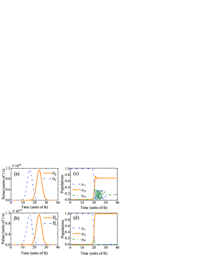
Figure 6: For ⁹⁷Tc, pulse shapes for (a) STIRAP and (b) effective two-level shortcut schemes. The populations as a function of time for (c) STIRAP and (d) effective two-level shortcut scheme are also compared.

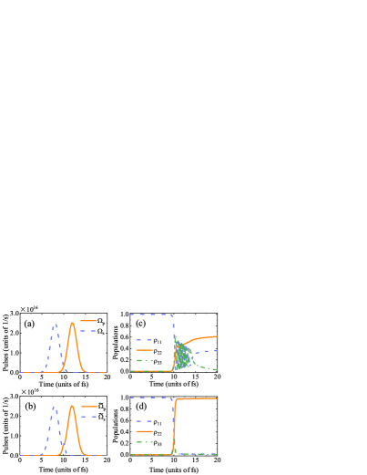
Figure 7: For ¹⁵⁴Gd, pulse shapes for (a) STIRAP and (b) effective two-level shortcut schemes. The populations as a function of time for (c) STIRAP and (d) effective two-level shortcut scheme are also compared.

We choose ⁹⁷Tc and ¹⁵⁴Gd as examples. The newly designed pump and Stokes pulses based on the effective two-level shortcut scheme, as compared to the STIRAP are shown in Figs. 6 and 7. The modified pulses are smooth enough to generate in the experiments, although they are different from standard Gaussian pulses. Both the peak value of modified pump and Stokes pulses and the operation time are greater than those in MIE. The real intensities of XFEL pulses are $I_{p}$=1 $\times$ 10²³ W/cm², $I_{s}$=2.3514 $\times$ 10²⁴ W/cm² and $I_{p}$=7.8927 $\times$ 10²¹ W/cm², $I_{s}$=1.4175 $\times$ 10²¹ W/cm² for ⁹⁷Tc and ¹⁵⁴Gd, respectively. The evolution of the states in Figs. 6 (c)-(d) and 7 (c)-(d) illustrate that high-fidelity population transfer can be achieved by using modified pulses, while the previous STIRAP does not work perfectly. When the lifetime of the excited state exceeds laser-nucleus interaction time, spontaneous emission can be neglected. The system can also be considered as a closed system. Thus, both ⁹⁷Tc and ¹⁵⁴Gd achieve almost 100$\%$ transfer efficiency. This equivalent treatment can still achieve high transfer efficiencies while providing a viable way to experimentally control nuclear states.

IV CONCLUSION

In summary, we have investigated a cyclic three-level nuclear system formed by direct coupling of the initial state $|1\rangle$ and the target state $|2\rangle$ with an additional laser field. Taking into account the effect of spontaneous emission from the intermediate excited state, we have mainly discussed the nuclear population transfer. The laser external field and instantaneous steady state of the system have been solved based on the MIE scheme. The performance of the MIE has been analysed using eight nuclei as examples, including excited state lifetimes longer (²²⁹Th,²²³Ra,¹¹³Cd,⁹⁷Tc), similar or shorter (¹⁸⁷Re,¹⁵⁴Gd,¹⁷²Yb,¹⁶⁸Er) than the laser-nucleus interaction time. Compared to STIRAP, one of the main significant advantages of the MIE is the shorter time required and the lower laser intensity. Each of the eight given nuclei can be transferred with high fidelity. This is because the additional field effectively inhibits the population of the intermediate excited state, thus avoiding the effects of spontaneous emission. The MIE scheme provides a practical, fast, and efficient means of controlling nuclear states. Another advantage is the robustness when the laser field parameters are changed. In particular, the transfer efficiency can be significantly improved by selecting the appropriate additional driving field, even when the intensities of the pump and Stokes fields are exceedingly low, without the need for powerful pump and Stokes fields. Furthermore, focusing on the absence of additional coupling between the initial and final levels, we have reduced the three-level system to an effective two-level system. By modifying the shape of the pump and Stokes pulses based on counterdiabatic driving, complete transfer has also been achieved. Our results bring a new perspective to the coherent manipulation of nuclear states, which is valuable for achieving the high-fidelity and controllable manipulation of nuclear states.

Appendix A THE DETAILS OF MIE SCHEME

The detailed procedure for obtaining laser field control parameters using the MIE scheme is given in this appendix. The explicit form of the density matrix is

$$\rho(t)=\begin{pmatrix}\rho_{11}&\rho_{12}&\rho_{13}\\ \rho_{21}&\rho_{22}&\rho_{23}\\ \rho_{31}&\rho_{32}&\rho_{33}\end{pmatrix}.$$ (27)

Substituting Eqs. (3) and (7) into Eq. (2), we obtain

$$\begin{aligned} \partial_{t}\rho_{11}&=\frac{i}{2}\Omega_{p}\rho_{13}-\frac{i}{2}\Omega_{p}\rho_{31}+\Gamma B_{31}\rho_{33},\\ \partial_{t}\rho_{12}&=\frac{i}{2}\Omega_{s}\rho_{13}-\frac{i}{2}\Omega_{p}\rho_{32},\\ \partial_{t}\rho_{13}&=\frac{i}{2}\Omega_{p}\rho_{11}+\frac{i}{2}\Omega_{s}\rho_{12}-\frac{1}{2}\Gamma\rho_{13}-\frac{i}{2}\Omega_{p}\rho_{33},\\ \partial_{t}\rho_{21}&=\frac{i}{2}\Omega_{p}\rho_{23}-\frac{i}{2}\Omega_{s}\rho_{31},\\ \partial_{t}\rho_{22}&=\frac{i}{2}\Omega_{s}\rho_{23}-\frac{i}{2}\Omega_{s}\rho_{32}+\Gamma B_{32}\rho_{33},\\ \partial_{t}\rho_{23}&=\frac{i}{2}\Omega_{p}\rho_{21}+\frac{i}{2}\Omega_{s}\rho_{22}-\frac{1}{2}\Gamma\rho_{23}-\frac{i}{2}\Omega_{s}\rho_{33},\\ \partial_{t}\rho_{31}&=-\frac{i}{2}\Omega_{p}\rho_{11}-\frac{i}{2}\Omega_{s}\rho_{21}-\frac{1}{2}\Gamma\rho_{31}+\frac{i}{2}\Omega_{p}\rho_{33},\\ \partial_{t}\rho_{32}&=-\frac{i}{2}\Omega_{p}\rho_{12}-\frac{i}{2}\Omega_{s}\rho_{22}-\frac{1}{2}\Gamma\rho_{32}+\frac{i}{2}\Omega_{s}\rho_{33},\\ \partial_{t}\rho_{33}&=-\frac{i}{2}\Omega_{p}\rho_{13}-\frac{i}{2}\Omega_{s}\rho_{23}+\frac{i}{2}\Omega_{p}\rho_{31}+\frac{i}{2}\Omega_{s}\rho_{32}-\Gamma\rho_{33}.\\ \end{aligned}$$ (28)

Apparently, the master equation in Eq. (2) can be rewritten as follows

$$\frac{\partial|\rho\rangle\rangle}{\partial t}=\hat{\mathcal{L}}(t)|\rho\rangle\rangle.$$ (29)

where

$$\hat{\mathcal{L}}(t)=\frac{1}{2}\begin{pmatrix}0&0&i\Omega_{p}&0&0&0&-i\Omega_{p}&0&2\Gamma B_{31}\\ 0&0&i\Omega_{s}&0&0&0&0&-i\Omega_{p}&0\\ i\Omega_{p}&i\Omega_{s}&-\Gamma&0&0&0&0&0&-i\Omega_{p}\\ 0&0&0&0&0&i\Omega_{p}&-i\Omega_{s}&0&0\\ 0&0&0&0&0&i\Omega_{s}&0&-i\Omega_{s}&2\Gamma B_{32}\\ 0&0&0&i\Omega_{p}&i\Omega_{s}&-\Gamma&0&0&-i\Omega_{s}\\ -i\Omega_{p}&0&0&-i\Omega_{s}&0&0&-\Gamma&0&i\Omega_{p}\\ 0&-i\Omega_{p}&0&0&-i\Omega_{s}&0&0&-\Gamma&i\Omega_{s}\\ 0&0&-i\Omega_{p}&0&0&-i\Omega_{s}&i\Omega_{p}&i\Omega_{s}&-2\Gamma\end{pmatrix}.$$ (30)

Here, we parameterize the instantaneous steady state using the generalized Bloch vector $\{r_{i}\}_{i=1}^{8}$. The density matrix of the three-level system is

$$\rho(t)=\frac{1}{3}(I+\sqrt{3}\sum_{i=1}^{8}r_{i}(t)T_{i}),$$ (31)

with $I$ is a $3\times 3$ identity matrix and the $T_{i}$ are the regular Gellmann matrices. The Bloch vectors corresponding to the instantaneous steady state are

$$\begin{aligned} r_{1}=-\sqrt{3}\frac{\Omega_{p}\Omega_{s}}{\Omega_{p}^{2}+\Omega_{s}^{2}},r_{3}=\frac{\sqrt{3}}{2}\frac{\Omega_{s}^{2}-\Omega_{p}^{2}}{\Omega_{p}^{2}+\Omega_{s}^{2}},r_{8}=\frac{1}{2},\end{aligned}$$ (32)

where $\overrightarrow{r}=(r_{1},r_{2},\dots,r_{8})$ is the generalized Bloch vector and the other components are zeros. Correspondingly, the dynamical invariant can be parameterized by the Bloch vector

$$\hat{\mathcal{I}}(t)=\begin{pmatrix}\frac{1}{3}(1+\sqrt{3}r_{3}+r_{8})&0&0&0&\frac{1}{3}(1+\sqrt{3}r_{3}+r_{8})&0&0&0&\frac{1}{3}(1+\sqrt{3}r_{3}+r_{8})\\ \frac{1}{\sqrt{3}}r_{1}&0&0&0&\frac{1}{\sqrt{3}}r_{1}&0&0&0&\frac{1}{\sqrt{3}}r_{1}\\ 0&0&0&0&0&0&0&0&0\\ \frac{1}{\sqrt{3}}r_{1}&0&0&0&\frac{1}{\sqrt{3}}r_{1}&0&0&0&\frac{1}{\sqrt{3}}r_{1}\\ \frac{1}{3}(1-\sqrt{3}r_{3}+r_{8})&0&0&0&\frac{1}{3}(1-\sqrt{3}r_{3}+r_{8})&0&0&0&\frac{1}{3}(1-\sqrt{3}r_{3}+r_{8})\\ 0&0&0&0&0&0&0&0&0\\ 0&0&0&0&0&0&0&0&0\\ 0&0&0&0&0&0&0&0&0\\ \frac{1}{3}(1-2r_{8})&0&0&0&\frac{1}{3}(1-2r_{8})&0&0&0&\frac{1}{3}(1-2r_{8})\end{pmatrix}.$$ (33)

Similar to Eq. (29), we can write Eq. (14) as

$$\frac{\partial|\rho\rangle\rangle}{\partial t}=\hat{\mathcal{L}}_{c}(t)|\rho\rangle\rangle.$$ (34)

with,

$$\hat{\mathcal{L}}_{c}(t)=\frac{1}{2}\begin{pmatrix}0&\Omega_{c}&i\Omega_{p}{{}^{\prime}}&\Omega_{c}&0&0&-i\Omega_{p}{{}^{\prime}}&0&2\Gamma B_{31}\\ -\Omega_{c}&0&i\Omega_{s}{{}^{\prime}}&0&\Omega_{c}&0&0&-i\Omega_{p}{{}^{\prime}}&0\\ i\Omega_{p}{{}^{\prime}}&i\Omega_{s}{{}^{\prime}}&-\Gamma&0&0&\Omega_{c}&0&0&-i\Omega_{p}{{}^{\prime}}\\ -\Omega_{c}&0&0&0&\Omega_{c}&i\Omega_{p}{{}^{\prime}}&-i\Omega_{s}{{}^{\prime}}&0&0\\ 0&-\Omega_{c}&0&-\Omega_{c}&0&i\Omega_{s}{{}^{\prime}}&0&-i\Omega_{s}{{}^{\prime}}&2\Gamma B_{32}\\ 0&0&-\Omega_{c}&i\Omega_{p}{{}^{\prime}}&i\Omega_{s}{{}^{\prime}}&-\Gamma&0&0&-i\Omega_{s}{{}^{\prime}}\\ -i\Omega_{p}{{}^{\prime}}&0&0&-i\Omega_{s}{{}^{\prime}}&0&0&-\Gamma&\Omega_{c}&i\Omega_{p}{{}^{\prime}}\\ 0&-i\Omega_{p}{{}^{\prime}}&0&0&-i\Omega_{s}{{}^{\prime}}&0&-\Omega_{c}&-\Gamma&i\Omega_{s}{{}^{\prime}}\\ 0&0&-i\Omega_{p}{{}^{\prime}}&0&0&-i\Omega_{s}{{}^{\prime}}&i\Omega_{p}{{}^{\prime}}&i\Omega_{s}{{}^{\prime}}&-2\Gamma\end{pmatrix}.$$ (35)

Considering all the above, upon substituting the aforementioned expression into the invariance conditions, the control parameters of the laser field can be deduced.

Appendix B THE CHARACTERISTIC PARAMETERS FOR NUCLEI

Table 1: The characteristic parameters for nuclei. $E_{i}$ is the energy of state $|i\rangle$ $(i=1,2,3)$ (in keV). $\gamma$ denotes relativistic factor. $\Gamma$ is the linewidth of state $|3\rangle$ (in meV). $B_{31}$ and $B_{32}$ are branching ratios of $|3\rangle\to|i\rangle(i=1,2)$, respectively. $\mu L_{ij}$, $\mu\in\{E,M\}$ are the multipolarities and $\mathbb{B}_{ij}(\mu L_{ij})$ (in Weisskopf units, wsu) denote the reduced matrix elements for the transitions $|i\rangle\to|3\rangle(i=1,2)$. The peak intensities of pump and Stokes laser pulse (in W/cm²) have been given in Refs. Nedaee-Shakarab et al. (2016); Kirschbaum et al. (2022).

Nucleus	$E_{3}$	$E_{2}$	$E_{1}$	$\gamma$	$\Gamma$	Branching ratio		Multipolarity		$\mathbb{B}_{13}$	$\mathbb{B}_{23}$	$\Omega_{p0}$	$\Omega_{s0}$	$I_{p}$ $\times$1021	$I_{s}$ $\times$1021
	(keV)	(keV)	(keV)		(meV)	$B_{31}$	$B_{32}$	$L_{13}$	$L_{23}$	(wsu)	(wsu)	(1/s)	(1/s)	(W/cm2)	(W/cm2)
229Th	29.19	8.19	0.00	1.18	5.45	0.0936	0.9250	$M1$	$E2$	0.003	44.9	$2.7174$ $\times$103	$8.5621$ $\times$103	$0.2750$	$0.0277$
223Ra	50.13	29.86	0.00	2.1	0.00144	0.9728	0.0272	$E1$	$E2$	0.00119	5.0	$4.1435$ $\times$103	$3.2895$ $\times$103	$5.7002$	$0.9044$
113Cd	522.26	263.54	263.54	10.5	0.00145	0.9879	0.1205	$E2$	$E1$	44.20	0.019	$6.2099$ $\times$103	$4.803$ $\times$102	$7.1528$	$1195.8$
97Tc	567.00	324.00	96.57	22.6	0.61	0.9653	0.0058	$E2$	$E1$	500	0.67	$3.5811$ $\times$104	$7.385$ $\times$103	$1.0000$	$23.514$
187Re	844.7	206.247	0.00	34.1	134.298	0.9978	0.0062	$E2$	$E2$	13000	80	$1.2585$ $\times$104	$4.8558$ $\times$104	$18.400$	$1.2360$
172Yb	1599.87	78.74	0.00	64.5	42.50	0.3911	0.6017	$E1$	$E1$	0.0018	12.3	$7.6374$ $\times$104	$1.4114$ $\times$105	$1.7923$	$0.5248$
168Er	1786.00	79.00	0.00	72	133.16	0.2908	0.7092	$E1$	$E1$	32	91	$1.1279$ $\times$105	$4.253$ $\times$105	$1.0241$	$0.0720$
154Gd	1241.00	123.00	0.00	50.1	300	0.5167	0.4752	$E1$	$E1$	0.044	490	$2.8268$ $\times$105	$6.6704$ $\times$105	$0.0790$	$0.0142$

References

- Di Piazza et al. (2012) A. Di Piazza, C. Müller, K. Z. Hatsagortsyan, and C. H. Keitel, Rev. Mod. Phys. 84, 1177 (2012).
- Leskowitz and Mueller (2004) G. M. Leskowitz and L. J. Mueller, Phys. Rev. A 69, 052302 (2004).
- Leuenberger et al. (2002) M. N. Leuenberger, D. Loss, M. Poggio, and D. D. Awschalom, Phys. Rev. Lett. 89, 207601 (2002).
- Stetcu et al. (2022) I. Stetcu, A. Baroni, and J. Carlson, Phys. Rev. C 105, 064308 (2022).
- Zhang et al. (2021a) D.-B. Zhang, H. Xing, H. Yan, E. Wang, and S.-L. Zhu, Chin. Phys. B 30, 020306 (2021a).
- Yeter-Aydeniz et al. (2020) K. Yeter-Aydeniz, R. C. Pooser, and G. Siopsis, npj Quantum Inf. 6, 63 (2020).
- Vandersypen and Chuang (2005) L. M. K. Vandersypen and I. L. Chuang, Rev. Mod. Phys. 76, 1037 (2005).
- Roggero et al. (2020) A. Roggero, C. Gu, A. Baroni, and T. Papenbrock, Phys. Rev. C 102, 064624 (2020).
- Aprahamian and Sun (2005) A. Aprahamian and Y. Sun, Nat. Phys. 1, 81 (2005).
- Carroll (2004) J. J. Carroll, Laser Phys. Lett. 1, 275 (2004).
- Belic et al. (1999) D. Belic, C. Arlandini, J. Besserer, J. de Boer, J. J. Carroll, J. Enders, T. Hartmann, F. Käppeler, H. Kaiser, U. Kneissl, M. Loewe, H. J. Maier, H. Maser, P. Mohr, P. von Neumann-Cosel, A. Nord, H. H. Pitz, A. Richter, M. Schumann, S. Volz, and A. Zilges, Phys. Rev. Lett. 83, 5242 (1999).
- Walker and Dracoulis (1999) P. Walker and G. Dracoulis, Nature 399, 35 (1999).
- Pálffy et al. (2007) A. Pálffy, J. Evers, and C. H. Keitel, Phys. Rev. Lett. 99, 172502 (2007).
- Walker et al. (2001) P. M. Walker, G. D. Dracoulis, and J. J. Carroll, Phys. Rev. C 64, 061302 (2001).
- Peik et al. (2021) E. Peik, T. Schumm, M. S. Safronova, A. Pálffy, J. Weitenberg, and P. G. Thirolf, Quantum Sci. Technol. 6, 034002 (2021).
- Seiferle et al. (2019) B. Seiferle, L. von der Wense, P. V. Bilous, I. Amersdorffer, C. Lemell, F. Libisch, S. Stellmer, T. Schumm, C. E. Düllmann, A. Pálffy, and P. G. Thirolf, Nature 573, 243 (2019).
- Kazakov et al. (2012) G. A. Kazakov, A. N. Litvinov, V. I. Romanenko, L. P. Yatsenko, A. V. Romanenko, M. Schreitl, G. Winkler, and T. Schumm, New J. Phys. 14, 083019 (2012).
- Beeks et al. (2021) K. Beeks, T. Sikorsky, T. Schumm, J. Thielking, M. V. Okhapkin, and E. Peik, Nat. Rev. Phys. 3, 238 (2021).
- Campbell et al. (2012) C. J. Campbell, A. G. Radnaev, A. Kuzmich, V. A. Dzuba, V. V. Flambaum, and A. Derevianko, Phys. Rev. Lett. 108, 120802 (2012).
- Feldhaus et al. (1997) J. Feldhaus, E. Saldin, J. Schneider, E. Schneidmiller, and M. Yurkov, Opt. Commun. 140, 341 (1997).
- Saldin et al. (2001) E. Saldin, E. Schneidmiller, Y. Shvyd’ko, and M. Yurkov, Nucl. Instrum. Methods Phys. Res., Sect. A 475, 357 (2001).
- Wootton et al. (2002) A. Wootton, J. Arthur, T. Barbee, R. Bionta, A. Jankowski, R. London, D. Ryutov, R. Shepherd, V. Shlyaptsev, R. Tatchyn, and A. Toor, Phys. Res., Sect. A 483, 345 (2002).
- Huang et al. (2021) N. Huang, H. Deng, B. Liu, D. Wang, and Z. Zhao, Innovation 2, 100097 (2021).
- Pellegrini et al. (2016) C. Pellegrini, A. Marinelli, and S. Reiche, Rev. Mod. Phys. 88, 015006 (2016).
- Altarelli (2011) M. Altarelli, Phys. Res., Sect. B 269, 2845 (2011).
- Wong et al. (2011) I. Wong, A. Grigoriu, J. Roslund, T.-S. Ho, and H. Rabitz, Phys. Rev. A 84, 053429 (2011).
- Bürvenich et al. (2006a) T. J. Bürvenich, J. Evers, and C. H. Keitel, Phys. Rev. C 74, 044601 (2006a).
- Liao and Pálffy (2014) W.-T. Liao and A. Pálffy, Phys. Rev. Lett. 112, 057401 (2014).
- Gunst et al. (2015) J. Gunst, Y. Wu, N. Kumar, C. H. Keitel, and A. Pálffy, Phys. Plasmas 22, 112706 (2015).
- Junker et al. (2012) A. Junker, A. Pálffy, and C. H. Keitel, New J. Phys. 14, 085025 (2012).
- von der Wense et al. (2020) L. von der Wense, P. V. Bilous, B. Seiferle, S. Stellmer, J. Weitenberg, P. G. Thirolf, A. Pálffy, and G. Kazakov, Eur. Phys. J. A 56, 176 (2020).
- Pálffy et al. (2015) A. Pálffy, O. Buss, A. Hoefer, and H. A. Weidenmüller, Phys. Rev. C 92, 044619 (2015).
- Di Piazza et al. (2007) A. Di Piazza, K. Hatsagortsyan, J. Evers, and C. Keitel, in Noise and Fluctuations in Photonics, Quantum Optics, and Communications (SPIE, 2007) pp. 20–30.
- Bürvenich et al. (2006b) T. J. Bürvenich, J. Evers, and C. H. Keitel, Phys. Rev. Lett. 96, 142501 (2006b).
- Liao (2014) W.-T. Liao, “Nuclear coherent population transfer with x-ray laser pulses,” in Coherent Control of Nuclei and X-Rays (Springer International Publishing, Cham, 2014) pp. 27–48.
- Amiri and Niari (2023) M. Amiri and M. S. Niari, Eur. Phys. J. A 59, 32 (2023).
- Chen et al. (2022) Y.-H. Chen, P.-H. Lin, G.-Y. Wang, A. Pálffy, and W.-T. Liao, Phys. Rev. Res. 4, L032007 (2022).
- Pálffy et al. (2011) A. Pálffy, C. H. Keitel, and J. Evers, Phys. Rev. B 83, 155103 (2011).
- Liao et al. (2013) W. T. Liao, A. Pálffy, and C. H. Keitel, Phys. Rev. C 87, 054609 (2013).
- Nedaee-Shakarab et al. (2016) B. Nedaee-Shakarab, M. Saadati-Niari, and F. Zolfagharpour, Phys. Rev. C 94, 054601 (2016).
- Liao et al. (2011) W. T. Liao, A. Pálffy, and C. H. Keitel, Phys. Lett. B 705, 134 (2011).
- Kirschbaum et al. (2022) T. Kirschbaum, N. Minkov, and A. Pálffy, Phys. Rev. C 105, 064313 (2022).
- Mansourzadeh-Ashkani et al. (2021a) N. Mansourzadeh-Ashkani, M. Saadati-Niari, F. Zolfagharpour, and B. Nedaee-Shakarab, Nucl. Phys. A 1007, 122119 (2021a).
- Nedaee-Shakarab et al. (2017) B. Nedaee-Shakarab, M. Saadati-Niari, and F. Zolfagharpour, Phys. Rev. C 96, 044619 (2017).
- Mansourzadeh-Ashkani et al. (2021b) N. Mansourzadeh-Ashkani, M. Saadati-Niari, F. Zolfagharpour, and B. Nedaee-Shakarab, J. Phys. G: Nucl. Part. Phys. 49, 015103 (2021b).
- Amiri and Saadati-Niari (2023) M. Amiri and M. Saadati-Niari, Phys. Scr. 98, 085303 (2023).
- Bergmann et al. (1998) K. Bergmann, H. Theuer, and B. W. Shore, Rev. Mod. Phys. 70, 1003 (1998).
- Bergmann et al. (2019) K. Bergmann, H.-C. Nägerl, C. Panda, G. Gabrielse, E. Miloglyadov, M. Quack, G. Seyfang, G. Wichmann, S. Ospelkaus, A. Kuhn, S. Longhi, A. Szameit, P. Pirro, B. Hillebrands, X.-F. Zhu, J. Zhu, M. Drewsen, W. K. Hensinger, S. Weidt, T. Halfmann, H.-L. Wang, G. S. Paraoanu, N. V. Vitanov, J. Mompart, T. Busch, T. J. Barnum, D. D. Grimes, R. W. Field, M. G. Raizen, E. Narevicius, M. Auzinsh, D. Budker, A. Pálffy, and C. H. Keitel, J. Phys. B: At. Mol. Opt. Phys. 52, 202001 (2019).
- Wu et al. (2021) S. Wu, W. Ma, X. Huang, and X. Yi, Phys. Rev. Appl. 16, 044028 (2021).
- Wang et al. (2024) M. Z. Wang, W. Ma, and S. L. Wu, Sci. Rep. 14, 3409 (2024).
- Vitanov and Stenholm (1997) N. V. Vitanov and S. Stenholm, Phys. Rev. A 55, 648 (1997).
- Zhang et al. (2021b) F.-Y. Zhang, Z.-Q. Feng, and C. Li, Commun. Theor. Phys. 73, 025105 (2021b).
- Li and Chen (2016) Y.-C. Li and X. Chen, Phys. Rev. A 94, 063411 (2016).
- Scully and Zubairy (1997) M. O. Scully and M. S. Zubairy, Quantum optics (Cambridge university press, 1997).
- Pálffy et al. (2008) A. Pálffy, J. Evers, and C. H. Keitel, Phys. Rev. C 77, 044602 (2008).
- Wu et al. (2019) S. L. Wu, X. L. Huang, and X. X. Yi, Phys. Rev. A 99, 042115 (2019).
- Lu et al. (2013) X. J. Lu, X. Chen, A. Ruschhaupt, D. Alonso, S. Guérin, and J. G. Muga, Phys. Rev. A 88, 033406 (2013).
- Venuti et al. (2016) L. C. Venuti, T. Albash, D. A. Lidar, and P. Zanardi, Phys. Rev. A 93, 032118 (2016).
- Sarandy et al. (2007) M. S. Sarandy, E. I. Duzzioni, and M. H. Y. Moussa, Phys. Rev. A 76, 052112 (2007).
- Kim et al. (2008) K. J. Kim, Y. Shvyd’ko, and S. Reiche, Phys. Rev. Lett. 100, 244802 (2008).
- Lindberg et al. (2011) R. R. Lindberg, K.-J. Kim, Y. Shvyd’ko, and W. M. Fawley, Phys. Rev. ST Accel. Beams 14, 010701 (2011).
- Blekos et al. (2020) K. Blekos, D. Stefanatos, and E. Paspalakis, Phys. Rev. A 102, 023715 (2020).
- Taddei et al. (2013) M. M. Taddei, B. M. Escher, L. Davidovich, and R. L. de Matos Filho, Phys. Rev. Lett. 110, 050402 (2013).
- Caneva et al. (2009) T. Caneva, M. Murphy, T. Calarco, R. Fazio, S. Montangero, V. Giovannetti, and G. E. Santoro, Phys. Rev. Lett. 103, 240501 (2009).
- Chen et al. (2010) X. Chen, I. Lizuain, A. Ruschhaupt, D. Guéry-Odelin, and J. G. Muga, Phys. Rev. Lett. 105, 123003 (2010).