Fourier optimization, the least quadratic non-residue, and the least prime in an arithmetic progression

Abstract.

By means of a Fourier optimization framework, we improve the current asymptotic bounds under GRH for two classical problems in number theory: the problem of estimating the least quadratic non-residue modulo a prime, and the problem of estimating the least prime in an arithmetic progression.

1. Introduction

In this paper, we apply a Fourier optimization framework to study two classical problems in number theory: (i) the problem of estimating the least quadratic non-residue modulo a prime, and (ii) the problem of estimating the least prime in an arithmetic progression. We are interested in establishing the strongest possible asymptotic bounds under the assumption of the Generalized Riemann Hypothesis (GRH) for Dirichlet $L$-functions. Our results are inspired by the previous work of Lamzouri, Li, and Soundararajan [25], who studied the same problems, and of Carneiro, Milinovich, and Soundararajan [12], who developed a Fourier optimization framework to study the maximum gap between primes assuming the Riemann Hypothesis. We provide a subtle, yet conceptually interesting, improvement on the results in [25]. One of the key elements of our approach is a thorough study of the extremal problems in Fourier analysis associated to these number theory problems. Throughout the paper we adopt the following normalization for the Fourier transform of a function $F\in L^{1}(\mathbb{R})$:

$$\widehat{F}(t):=\int_{-\infty}^{\infty}e^{-2\pi ixt}\,F(x)\,\text{\rm d}x.$$

1.1. The least quadratic non-residue

Let $p$ be an odd prime, and let $n_{p}$ denote the least quadratic non-residue modulo $p$. As a consequence of the Pólya-Vinogradov inequality, I. M. Vinogradov developed a clever trick that established the bound $n_{p}\ll p^{\frac{1}{2\sqrt{e}}}\log^{2}p$. Burgess later combined Vinogradov’s trick with his bounds for character sums to show that $n_{p}=O_{\varepsilon}\big{(}p^{\frac{1}{4\sqrt{e}}+\varepsilon}\big{)}$ for all $\varepsilon>0$. Vinogradov further conjectured that $n_{p}\ll_{\varepsilon}p^{\varepsilon}$ for all $\varepsilon>0$, and Vinogradov’s conjecture is now known to follow from the generalized Lindelöf hypothesis and therefore from GRH.

Under GRH, Ankeny [1] proved that $n_{p}\ll\log^{2}p$. The order of magnitude of this estimate has never been improved. Bach [2] later established the asymptotic estimate $n_{p}\leq(1+o(1))\log^{2}p$ which was improved by Lamzouri, Li, and Soundararajan [25, 26] to $n_{p}\leq(0.794+o(1))\log^{2}p$.

We consider here the following constant arising from a Fourier optimization problem:

$$\mathcal{C}(1):=\sup_{0\neq F\in\mathcal{A}}\frac{2\pi}{\|F\|_{1}}\left(\int_{-\infty}^{0}\widehat{F}(t)\,e^{\pi t}\,\text{\rm d}t-\int_{0}^{\infty}\big{|}\widehat{F}(t)\big{|}\,e^{\pi t}\,\text{\rm d}t\right),$$ (1.1)

where the supremum is taken over the class of functions $\mathcal{A}=\{F:\mathbb{R}\to\mathbb{C}\,;\ F\in L^{1}(\mathbb{R})\,;\ \widehat{F}\ {\rm is\ real\mbox{-}valued}\}$. We improve the current best conditional bounds for the least quadratic non-residue by establishing the following connection.

Theorem 1.

Assume GRH. Let $n_{p}$ be the least quadratic non-residue modulo a prime $p$. Then

$$\limsup_{p\to\infty}\frac{n_{p}}{\log^{2}p}\leq\mathcal{C}(1)^{-2}<0.7615\,.$$

This result is a particular case of our more general Theorem 6, below. We also note that the bound in Theorem 5 shows that $\mathcal{C}(1)^{-2}>0.7596$, which shows that we have essentially arrived at the limit of this method. In other words, assuming GRH, we prove that $n_{p}<\frac{61}{80}\log^{2}p$ when $p$ is sufficiently large, but that replacing $\frac{61}{80}$ by $\frac{3}{4}$ is not possible using our method.

It is not difficult to see that the least quadratic non-residue $n_{p}$ must be prime. Given this fact, it is also natural to study the size of least prime quadratic residue modulo $p$, which we denote by $r_{p}$. Analogous to his conjecture for $n_{p}$, I. M. Vinogradov conjectured that $r_{p}\ll_{\varepsilon}p^{\varepsilon}$ for any $\varepsilon>0$. The Pólya-Vinogradov inequality and Siegel’s theorem for exceptional zeros of Dirichlet $L$-functions imply that $r_{p}\ll_{\varepsilon}p^{1/2+\varepsilon}$. Yu. V. Linnik and A. I. Vinogradov [35] used Burgess’ bounds for character sums and Siegel’s theorem to show that $r_{p}\ll_{\varepsilon}p^{1/4+\varepsilon}$. The implied constants in both of these bounds are ineffective. Assuming GRH, Ankeny [1] proved that $r_{p}\ll\log^{2}p$ and the order of magnitude of this estimate has never been improved. We modify our proof of Theorem 1 to prove the following result.

Theorem 2.

Assume GRH. Let $r_{p}$ be the least prime quadratic residue modulo a prime $p$. Then

$$\limsup_{p\to\infty}\frac{r_{p}}{\log^{2}p}\leq\mathcal{C}(1)^{-2}<0.7615\,.$$

1.2. The least prime in an arithmetic progression

For $q\in\mathbb{N}$ and $a\in\mathbb{Z}$ with $\gcd(a,q)=1$, let $P(a,q)$ be the least prime in the arithmetic progression $\equiv a\,({\rm mod}\,q)$. When it comes to unconditional bounds, a classical result of Linnik establishes that $P(a,q)\ll q^{L}$ for some universal constant $L$. Heath-Brown [23] showed that $L=5.5$ is an admissible value for Linnik’s constant, and this result was later improved to $L=5.2$ by Xylouris [36].

Under GRH, the asymptotic estimate $P(a,q)\leq(1+o(1))(\phi(q)\log q)^{2}$ was established by Bach and Sorensen [3], and the absolute bound $P(a,q)\leq(\phi(q)\log q)^{2}$, for $q>3$, was established by Lamzouri, Li and Soundararajan in [25]. It was suggested in [25] that a modification of their proof, with the use of the Brun-Titchmarsh inequality, would yield an asymptotic bound of the form $P(a,q)\leq(1-\delta+o(1))(\phi(q)\log q)^{2}$, for some small $\delta>0$. Our next result finds an explicit constant for this inequality, by relating it to the following constant arising from a Fourier optimization problem:

$$\mathcal{C}(3):=\sup_{0\neq F\in\mathcal{A}}\frac{2\pi}{\|F\|_{1}}\left(\int_{-\infty}^{0}\widehat{F}(t)\,e^{\pi t}\,\text{\rm d}t-\int_{0}^{\infty}\widehat{F}(t)\,e^{\pi t}\,\text{\rm d}t-2\int_{0}^{\infty}\big{|}\widehat{F}(t)\big{|}\,e^{\pi t}\,\text{\rm d}t\right),$$ (1.2)

where the supremum is taken over the class of functions $\mathcal{A}=\{F:\mathbb{R}\to\mathbb{C}\,;\ F\in L^{1}(\mathbb{R})\,;\ \widehat{F}\ {\rm is\ real\mbox{-}valued}\}$.

Theorem 3.

Assume GRH. Let $q\in\mathbb{N}$ and $a\in\mathbb{Z}$ with $\gcd(a,q)=1$. The least prime $P(a,q)$ that is congruent to $a$ modulo $q$ verifies

$$\limsup_{q\to\infty}\frac{P(a,q)}{(\phi(q)\log q)^{2}}\leq\mathcal{C}(3)^{-2}<\frac{8}{9}.$$ (1.3)

We note in Theorem 5 that $\mathcal{C}(3)^{-2}>0.8859$, which shows, as in the case of Theorem 1, that we are essentially at the limit of the method.

1.3. Fourier optimization

A Fourier optimization problem can generally be described as a problem in which one prescribes certain constraints for a function and its Fourier transform, and wants to optimize a certain quantity of interest. Some problems of this type turn out to be connected to problems in number theory and other fields, and establishing such bridges is usually an interesting part of the process. Recent examples of Fourier optimization problems arise in connection to: bounds for the modulus and argument of the Riemann zeta-function [7, 8, 13]; bounds related to Montgomery’s pair correlation conjecture [5, 6, 11, 21, 31]; the maximum size of gaps between primes [12, 15, 16]; the proportion of simple zeros of zeta and $L$-functions [14, 27, 33]; non-vanishing of $L$-functions at the central point and low-lying heights [9, 20, 30]; and the recent breakthroughs in the sphere packing problem and energy-minimizing point configurations [17, 18, 19, 22, 34].

Throughout the paper, for a real-valued function $G$, we let

$$G_{+}(x):=\max\{G(x),0\}\ \ \ {\rm and}\ \ \ G_{-}(x):=\max\{-G(x),0\}.$$

Then, one plainly has $G(x)=G_{+}(x)-G_{-}(x)$ and $|G(x)|=G_{+}(x)+G_{-}(x)$. We consider the following family of optimization problems parametrized by a real number $0\leq A<\infty$ or $A=\infty$.

Extremal Problem 1 $(EP1)$. Given $0\leq A<\infty$, find

$$\mathcal{C}(A):=\sup_{0\neq F\in\mathcal{A}}\frac{2\pi}{\|F\|_{1}}\left(\int_{-\infty}^{0}\widehat{F}(t)\,e^{\pi t}\,\text{\rm d}t-\int_{0}^{\infty}\widehat{F}_{-}(t)\,e^{\pi t}\,\text{\rm d}t-A\int_{0}^{\infty}\widehat{F}_{+}(t)\,e^{\pi t}\,\text{\rm d}t\right),$$ (1.4)

where the supremum is taken over the class of functions $\mathcal{A}=\{F:\mathbb{R}\to\mathbb{C}\,;\ F\in L^{1}(\mathbb{R})\,;\ \widehat{F}\ {\rm is\ real\mbox{-}valued}\}$. For $A=\infty$, find

$$\mathcal{C}(\infty):=\sup_{0\neq F\in\mathcal{A}_{\infty}}\frac{2\pi}{\|F\|_{1}}\left(\int_{-\infty}^{0}\widehat{F}(t)\,e^{\pi t}\,\text{\rm d}t-\int_{0}^{\infty}\widehat{F}_{-}(t)\,e^{\pi t}\,\text{\rm d}t\right),$$ (1.5)

where the supremum is taken over the subclass $\mathcal{A}_{\infty}\subset\mathcal{A}$ given by $\mathcal{A}_{\infty}=\{F:\mathbb{R}\to\mathbb{C}\,;\ F\in L^{1}(\mathbb{R})\,;\ \widehat{F}\ {\rm is\ real\mbox{-}valued}\,;\ \widehat{F}(t)\leq 0\ {\rm for}\ t\geq 0\}$.

As we shall see, the problem of estimating the least character non-residue, generalizing the least quadratic non-residue presented in Theorem 1, is connected to (EP1) in the cases $A=1/(\ell-1)$ for $\ell\in\mathbb{N}$, $\ell\geq 2$, and hence we pay a closer attention to this problem in the range $0\leq A\leq 1$. On the other hand, the problem of estimating the least prime in an arithmetic progression is connected to (EP1) in the case $A=3$, and we also pay attention to this case. Our next result collects some qualitative and quantitative properties of $\mathcal{C}(A)$.

Theorem 4.

The following propositions hold:

• The supremum in (1.4) - (1.5) restricted to the functions $F\in\mathcal{A}$ $($or $F\in\mathcal{A}_{\infty}$ in case $A=\infty$$)$ with $\widehat{F}\in C^{\infty}_{c}(\mathbb{R})$, still yields $\mathcal{C}(A)$.

• The function $A\mapsto\mathcal{C}(A)$ is continuous and non-increasing for $0\leq A\leq\infty$.

• One has the exact endpoint values ${\mathcal{C}}(0)=2$ and ${\mathcal{C}}(\infty)=1$.

• For $0\leq A<1$, one has the bound:

  $${\mathcal{C}}(A)\geq\max\left\{2+\frac{2\,(A\!+\!1)\log\left(\frac{3-A}{A+1}\right)}{\log A}+2A\ \,;\ \,1\right\}.$$ (1.6)

Remarks. (i) Noting that the maximum of $x\mapsto 2\,(x+1)\log\!\left(\frac{3-x}{x+1}\right)$ for $0\leq x<1$ occurs at $x=0$, from (1.6) one arrives at the weaker, yet simpler, lower bound

$${\mathcal{C}}(A)\geq 2+\frac{2\log 3}{\log A}\,,$$ (1.7)

which is asymptotically equivalent to (1.6) as $A\to 0$.

(ii) From a number theoretic viewpoint, the constant $A$ in our extremal problem (EP1) arises from (over)estimating the contributions of the primes beyond the least quadratic non-residue or the least prime in an arithmetic progression. In the case of the least quadratic non-residue, we arrive at $A=1$ using the Prime Number Theorem. In the case of the least prime in an arithmetic progression, we arrive at $A=3$ using the Brun-Titchmarsh Theorem. The case $A=\infty$ corresponds to the situation where no analogue of the Brun-Titchmarsh Theorem exists. Such a situation arises when one attempts to bound the least prime in the Chebotarev density theorem in a general setting. In particular, our result that ${\mathcal{C}}(\infty)=1$ can be used to show that the results of Bach and Sorensen [3, Theorem 3.1] concerning the least prime in the Chebotarev density theorem assuming the Extended Riemann Hypothesis are best possible using their method.

(iii) The Fourier analysis framework developed in this paper should be applicable to proving conditional estimates to a variety of arithmetic problems which rely on input from low-lying zeros of $L$-functions (once one has determined the appropriate constant $A$ for the problem).

Although our extremal problem (EP1) can be stated in accessible terms, one quickly realizes that the task of actually finding the exact value of the sharp constant $\mathcal{C}(A)$ is rather subtle in general. Our next result presents high precision upper and lower bounds for $\mathcal{C}(A)$ in the most interesting cases for our applications.

Theorem 5.

One has the following bounds:

$$1.31706 <\mathcal{C}(1/4)<1.33509;$$

$$1.27722 <\mathcal{C}(1/3)<1.28781;$$

$$1.22112 <\mathcal{C}(1/2)<1.23080;$$

$$1.14600 <\mathcal{C}(1)<1.14731;$$

$$1.06082 <\mathcal{C}(3)<1.06240.$$

Establishing upper bounds for $\mathcal{C}(A)$ is a somewhat delicate issue. Our strategy unveils a connection with a suitable auxiliary extremal problem. Once this bridge is in place, the work to establish upper and lower bounds in Theorem 5 is reduced to finding near-extremal test functions for both the original and the auxiliary extremal problems, a task that is performed via suitable robust programming routines. In principle, our method of proof of Theorem 5 could be adapted to treat, with high precision, any other particular fixed value of $A$.

1.4. The least character non-residue

Proceeding slightly more generally than in §1.1, let $q\in\mathbb{N}$ and let $\chi$ be a non-principal Dirichlet character modulo $q$. Set

$$n_{\chi}:=\min\{n\in\mathbb{N};\ \chi(n)\neq 0,1\}\,,$$ (1.8)

known as the least character non-residue. Under GRH, Ankeny [1] showed that $n_{\chi}\ll\log^{2}q$, and the absolute bound $n_{\chi}\leq\log^{2}q$, if $q$ is not divisible by any prime below $\log^{2}q$, was established by Lamzouri, Li, and Soundararajan in [25]. When it comes to asymptotic results, the uniform estimate $n_{\chi}\leq\big{(}1+o(1)\big{)}\log^{2}q$ was proved by Bach [2], and later refined in [25] to $n_{\chi}\leq\big{(}0.794+o(1)\big{)}\log^{2}q$. It was observed in [25] that one can do better if one knows, a priori, the order of the character $\chi$. For instance, if $\chi$ is cubic then $n_{\chi}\leq\big{(}0.7+o(1)\big{)}\log^{2}q$, and if $\chi$ is quartic then $n_{\chi}\leq\big{(}0.66+o(1)\big{)}\log^{2}q$. Our next result provides a sharpening of these inequalities, by relating them to the solution of the extremal problem (EP1).

Theorem 6.

Assume GRH. Let $q\in\mathbb{N}$ and let $\chi$ be a non-principal Dirichlet character modulo $q$ of order $\ell$. Then the least character non-residue $n_{\chi}$ satisfies

$$\limsup_{q\to\infty}\frac{n_{\chi}}{\log^{2}q}\leq\mathcal{C}\!\left(\frac{1}{\ell\!-\!1}\right)^{-2}.$$

From Theorem 5 and the lower bound (1.7) we immediately have the following corollary.

Corollary 7.

Under the same hypotheses of Theorem 6:

• If $\ell=2$, then $n_{\chi}\leq\big{(}0.7615+o(1)\big{)}\log^{2}q$.

• If $\ell=3$, then $n_{\chi}\leq\big{(}0.6707+o(1)\big{)}\log^{2}q$.

• If $\ell=4$, then $n_{\chi}\leq\big{(}0.6131+o(1)\big{)}\log^{2}q$.

• If $\ell=5$, then $n_{\chi}\leq\big{(}0.5765+o(1)\big{)}\log^{2}q$.

• For $\ell\geq 6$, one has

  $$\limsup_{q\to\infty}\frac{n_{\chi}}{\log^{2}q}\leq\frac{1}{4}\left(1-\frac{\log 3}{\log(\ell\!-\!1)}\right)^{-2}.$$ (1.9)

Remarks. (i) Theorem 5 shows that the upper bounds in Corollary 7 (i) - (iv) cannot be improved beyond $0.7596\ldots$, $0.6601\ldots$, $0.6029\ldots$ and $0.5610\ldots$, respectively, with this method.

(ii) We note that Theorem 1 is an immediate consequence of Theorem 6 and Corollary 7 upon letting $q$ be prime and letting $\chi$ be the Legendre symbol modulo $q$ (so that $\ell=2$).

Our strategy to prove Theorem 6 is inspired in the asymptotic bounds of the previous work of Lamzouri, Li, and Soundararajan in [25], with certain differences. Both here and in [25], the idea is to consider a character sum with values $1$ up to a certain point and then $-1$ from that point on (after a suitable cancellation provided by the order of the character). In [25], this is done via the Mellin transform and appropriate contour shifting, while here we alternatively work directly with the Fourier transform and explicit formulas. If one carefully translate the arguments of [25, Section 6] to the Fourier transform language via the appropriate changes of variables, one sees that the extremal problem setup in [25, Proposition 6.1] reduces to our (EP1), in the case $A=1/(\ell-1)$, after certain simplifications due to additional restrictions on the test functions. Precisely, in [25, Proposition 6.1] one assumes that $F$ is analytic in the strip $-\frac{1}{2}-\varepsilon<{\rm Im}(s)<\frac{1}{2}+\varepsilon$, that $|F(s)|\ll(1+|s|^{2})^{-1}$ in this strip as $|{\rm Re}(s)|\to\infty$, and that $\widehat{F}\geq 0$ on $\mathbb{R}$. The first two assumptions are harmless since we prove in Theorem 4 (i) that $F$ can be taken entire and Schwartz on $\mathbb{R}$ for (EP1). However, the additional assumption that $\widehat{F}\geq 0$ on $\mathbb{R}$ makes the two problems different. It is not clear that near-extremizers of problem (EP1) will have this property (most likely not; see the discussion in Section 5). Some of our test functions used in Theorem 5 already show a small oscillation of the sign of $\widehat{F}$, e.g. the test function for the lower bound when $A=1$.

Here we not only estimate the limit of the method in the particular situations of low order characters (Theorem 5) but also in the regime where the order $\ell$ is large. This is given by (1.9), in which one gets the constant $1/4$ as the limit. The same limiting constant $1/4$ was also obtained in [25, Theorem 1.3] with a slightly larger upper bound.

1.5. Structure of the paper

The rest of the paper, in which we prove the main results stated in this introduction, can be broadly divided into three independent parts:

• The analysis part. This is Section 2, where we prove Theorem 4.

• The number theory part. This is comprised of Sections 3 and 4, where we prove Theorem 6 and Theorem 3, respectively. At the end of Section 3, we briefly indicate the changes necessary in the proof of Theorem 3 that are needed in order to prove Theorem 2.

• The computational part. This is Section 5, where we discuss the computer-assisted proof of Theorem 5.

2. Extremal problems: proof of Theorem 4

Let us introduce another important tool in our conceptual framework, that shall be relevant not only for the proof of Theorem 4 but also for the proof of Theorem 5 in the upcoming Section 5.

2.1. An auxiliary extremal problem

Let ${\bf 1}_{\mathbb{R}_{-}}$ be the characteristic function of $(-\infty,0)$ and ${\bf 1}_{\mathbb{R}_{+}}$ be the characteristic function of $(0,\infty)$. We consider the following auxiliary problem.

Extremal Problem 2 $(EP2)$. Given $0\leq A\leq\infty$, find

$$\mathcal{C}^{*}(A)=\inf_{0\neq\psi\in\mathcal{B}_{A}}\ 2\pi\,\left\|\,\widehat{{\bf 1}_{\mathbb{R}_{-}}\,e^{\pi(\cdot)}}-\widehat{{\bf 1}_{\mathbb{R}_{+}}\,\psi}\,\right\|_{\infty}\,,$$

where the infimum is taken over the class $\mathcal{B}_{A}=\{\psi:\mathbb{R}_{+}\to\mathbb{R};\ \psi\in L^{1}(\mathbb{R}_{+})\ {\rm and}\ -e^{\pi t}\leq\psi(t)\leq A\,e^{\pi t}\ {\rm for\ all}\ t\in\mathbb{R}_{+}\}$.

Remark: If $A=\infty$, the last condition is understood simply as $-e^{\pi t}\leq\psi(t)$ for all $t\in\mathbb{R}_{+}$.

It is clear from the definition of the extremal problem (EP2) that the map $A\mapsto\mathcal{C}^{*}(A)$ is non-increasing. We prove the following relation between our extremal problems (EP1) and (EP2).

Proposition 8.

For each $0\leq A\leq\infty$ one has

$$\mathcal{C}(A)\leq\mathcal{C}^{*}(A).$$ (2.1)

Proof.

Let $0\neq F\in\mathcal{A}$ (or $0\neq F\in\mathcal{A}_{\infty}$ in case $A=\infty$) be given. Using the multiplication formula for the Fourier transform, for any $\psi\in\mathcal{B}_{A}$ we have

$$\int_{-\infty}^{0}\widehat{F}(t)\,e^{\pi t}\,\text{\rm d}t -\int_{0}^{\infty}\widehat{F}_{-}(t)\,e^{\pi t}\,\text{\rm d}t-A\int_{0}^{\infty}\widehat{F}_{+}(t)\,e^{\pi t}\,\text{\rm d}t\leq\int_{-\infty}^{\infty}\widehat{F}(t)\Big{(}{\bf 1}_{\mathbb{R}_{-}}(t)\,e^{\pi t}-{\bf 1}_{\mathbb{R}_{+}}(t)\,\psi(t)\Big{)}\,\text{\rm d}t$$

$$=\int_{-\infty}^{\infty}F(x)\Big{(}\widehat{{\bf 1}_{\mathbb{R}_{-}}\,e^{\pi(\cdot)}}-\widehat{{\bf 1}_{\mathbb{R}_{+}}\,\psi}\Big{)}(x)\,\text{\rm d}x\leq\|F\|_{1}\,\left\|\,\widehat{{\bf 1}_{\mathbb{R}_{-}}\,e^{\pi(\cdot)}}-\widehat{{\bf 1}_{\mathbb{R}_{+}}\,\psi}\,\right\|_{\infty}.$$

This plainly leads us to (2.1). ∎

2.2. Approximations: proof of Theorem 4 (i)

Our argument below works in both cases $0\leq A<\infty$ and $A=\infty$. Note first that $\mathcal{C}(A)>0$; to see this just take any test function $F\in\mathcal{A}$ with ${\rm supp}\big{(}\widehat{F}\big{)}\subset(-\infty,0]$. Start with any $0\neq F\in\mathcal{A}$ (resp. $0\neq F\in\mathcal{A}_{\infty}$ if $A=\infty$) and define

$$J_{A}(F):=\frac{2\pi}{\|F\|_{1}}\left(\int_{-\infty}^{0}\widehat{F}(t)\,e^{\pi t}\,\text{\rm d}t-\int_{0}^{\infty}\widehat{F}_{-}(t)\,e^{\pi t}\,\text{\rm d}t-A\int_{0}^{\infty}\widehat{F}_{+}(t)\,e^{\pi t}\,\text{\rm d}t\right)$$

(resp. with the last integral on the right removed if $A=\infty$). We may assume that $J_{A}(F)>0$. Let $K(x)=\big{(}\sin(\pi x)/(\pi x)\big{)}^{2}$ be the Fejér kernel and recall that $\widehat{K}(t)=(1-|t|)_{+}$. For $\varepsilon>0$, define $K_{\varepsilon}(x):=\varepsilon^{-1}K(x/\varepsilon)$. Since $\widehat{F*K_{\varepsilon}}(t)=\widehat{F}(t)\widehat{K}(\varepsilon t)$, an application of dominated convergence in the numerator, together with the fact that $\|F*K_{\varepsilon}\|_{1}\to\|F\|_{1}$ as $\varepsilon\to 0$, yields $\lim_{\varepsilon\to 0}J_{A}(F*K_{\varepsilon})=J_{A}(F)$. We may hence assume that our test function $F$ is bandlimited.

Let $\eta\in C^{\infty}_{c}(\mathbb{R})$ be an even and non-negative function with ${\rm supp}(\eta)\subset[-1,1]$ and $\int_{-1}^{1}\eta(x)\,\text{\rm d}x=1$. Again, for $\varepsilon>0$, let $\eta_{\varepsilon}(x):=\varepsilon^{-1}\eta(x/\varepsilon)$. Assume that ${\rm supp}(\widehat{F})\subset[-\Lambda,\Lambda]$ and define $F^{\varepsilon}(x):=F(x)\,\widehat{\eta}(\varepsilon x)\,e^{-2\pi ix\varepsilon}$. Then $\widehat{F^{\varepsilon}}(t)=\widehat{F}*\eta_{\varepsilon}(t+\varepsilon)\in C^{\infty}_{c}(\mathbb{R})$ and ${\rm supp}(\widehat{F^{\varepsilon}})\subset[-\Lambda-2\varepsilon,\Lambda]$ (this small translation by $\varepsilon$ is just to guarantee that $F^{\varepsilon}\in\mathcal{A}_{\infty}$ in case $F\in\mathcal{A}_{\infty}$). Note that $\|F^{\varepsilon}\|_{1}\to\|F\|_{1}$ as $\varepsilon\to 0$, by dominated convergence. Since $\widehat{F}$ is uniformly continuous, note that $\widehat{F^{\varepsilon}}\to\widehat{F}$ uniformly as $\varepsilon\to 0$, and hence $\widehat{F^{\varepsilon}}_{-}\to\widehat{F}_{-}$ and $\widehat{F^{\varepsilon}}_{+}\to\widehat{F}_{+}$ uniformly as well. Yet another application of dominated convergence in the numerator yields $\lim_{\varepsilon\to 0}J_{A}(F^{\varepsilon})=J_{A}(F)$. This concludes the proof of this part.

2.3. Continuity: proof of Theorem 4 (ii)

From the definition of the problem, it is clear that the function $A\mapsto\mathcal{C}(A)$ is non-increasing. Let us show that it is continuous up to $\infty$ (i.e. we also want to show that $\lim_{A\to\infty}\mathcal{C}(A)=\mathcal{C}(\infty)$).

For a fixed $0\leq A<\infty$, given $\varepsilon>0$, let $F\in\mathcal{A}$ be such that $J_{A}(F)\geq\mathcal{C}(A)-\varepsilon$. Then, by the continuity of the numerator, there exists $\delta=\delta(\varepsilon,F)>0$ such that if $|B-A|\leq\delta$ then $J_{B}(F)\geq J_{A}(F)-\varepsilon$. Hence $\mathcal{C}(B)\geq J_{B}(F)\geq J_{A}(F)-\varepsilon\geq\mathcal{C}(A)-2\varepsilon$. Since $\varepsilon>0$ was arbitrary, we get

$$\liminf_{B\to A}\mathcal{C}(B)\geq\mathcal{C}(A).$$ (2.2)

Since $A\mapsto\mathcal{C}(A)$ is non-increasing, note that (2.2) already implies that this map is continuous at $A=0$. Note also that (2.2) is trivially true for $A=\infty$.

Now assume that $0<A<\infty$ and let $\{A_{n}\}_{n\geq 1}$ be a sequence such that $A_{n}>0$ for each $n$ and $A_{n}\to A$ as $n\to\infty$. Let $F_{n}\in\mathcal{A}$ be normalized such that $\|F_{n}\|_{1}=1$ and $J_{A_{n}}(F_{n})\geq\mathcal{C}(A_{n})-\frac{1}{n}$. Since $\|\widehat{F_{n}}\|_{\infty}\leq\|F_{n}\|_{1}=1$,

$$\left|\int_{-\infty}^{0}\widehat{F_{n}}(t)\,e^{\pi t}\,\text{\rm d}t\right|\leq\int_{-\infty}^{0}e^{\pi t}\,\text{\rm d}t=\frac{1}{\pi},$$

and from the fact that $\mathcal{C}(A_{n})>0$ we obtain

$$A_{n}\int_{0}^{\infty}\big{(}\widehat{F_{n}}\big{)}_{+}(t)\,e^{\pi t}\,\text{\rm d}t\leq\frac{1}{\pi}.$$

Therefore,

$$\big{|}J_{A}(F_{n})-J_{A_{n}}(F_{n})\big{|}=2\pi\left|(A-A_{n})\int_{0}^{\infty}\big{(}\widehat{F_{n}}\big{)}_{+}(t)\,e^{\pi t}\,\text{\rm d}t\right|\leq\frac{2\,|A-A_{n}|}{A_{n}}\,,$$

and note that this last quantity goes to $0$ as $n\to\infty$. This plainly leads us to

$$\mathcal{C}(A)\geq\limsup_{n\to\infty}J_{A}(F_{n})=\limsup_{n\to\infty}J_{A_{n}}(F_{n})=\limsup_{n\to\infty}\mathcal{C}(A_{n}).$$ (2.3)

The desired continuity at $0<A<\infty$ then follows from (2.2) and (2.3).

The argument in the previous paragraph does not immediately work to prove the continuity at $A=\infty$ since the functions $F_{n}$ may not be in the class $\mathcal{A}_{\infty}$. We have to be a bit more careful in this case, and argue using the auxiliary extremal problem (EP2). We show that $\mathcal{C}^{*}(A)=1+o(1)$ as $A\to\infty$. Recall that

$$2\pi\,\widehat{{\bf 1}_{\mathbb{R}_{-}}\,e^{\pi(\cdot)}}(x)=\frac{2}{1-2ix}.$$

The intuitive idea is the following: if we consider $\psi=\frac{1}{2\pi}{\bm{\delta}}$, where ${\bm{\delta}}$ is the Dirac delta at the origin, we would have

$$2\pi\,\widehat{{\bf 1}_{\mathbb{R}_{-}}\,e^{\pi(\cdot)}}(x)-2\pi\,\widehat{\psi}(x)=\frac{2}{1-2ix}-1=\frac{1+2ix}{1-2ix}\,,$$

and hence $2\pi\big{\|}\,\widehat{{\bf 1}_{\mathbb{R}_{-}}\,e^{\pi(\cdot)}}-\widehat{\psi}\,\big{\|}_{\infty}=1$. With this target example in mind, we argue with a suitable admissible approximation. For $A$ large (and finite), let us choose a test function $\psi_{A}\in\mathcal{B}_{A}$ for (EP2) given by $\psi_{A}(t)=A\,{\bf 1}_{[0,1/(2\pi A)]}(t)$. Then, note that

$$2\pi\,\widehat{{\bf 1}_{\mathbb{R}_{+}}\,\psi_{A}}(x)=\frac{1-e^{-ix/A}}{ix/A}.$$

By the mean value inequality, $|1-e^{i\theta}|\leq|\theta|$ for $\theta\in\mathbb{R}$, and we get

$$\big{\|}2\pi\,\widehat{{\bf 1}_{\mathbb{R}_{+}}\,\psi_{A}}(x)\big{\|}_{\infty}\leq 1.$$ (2.4)

Also, note that $\lim_{x\to 0}2\pi\,\widehat{{\bf 1}_{\mathbb{R}_{+}}\,\psi_{A}}(x)=1$.

Now let $\varepsilon>0$ be given, and let $N=N(\varepsilon)$ be large so that

$$\left|\frac{2}{1-2ix}\right|\leq\varepsilon$$ (2.5)

if $|x|\geq N$. Fix $A_{0}=A_{0}(\varepsilon,N)$, so that if $A\geq A_{0}$ we have

$$\left|\frac{1-e^{-ix/A}}{ix/A}-1\right|\leq\varepsilon$$ (2.6)

if $|x|\leq N$. Hence, if $A\geq A_{0}$ and $|x|\leq N$, we use the triangle inequality and (2.6) to get

$$\left|2\pi\,\widehat{{\bf 1}_{\mathbb{R}_{-}}\,e^{\pi(\cdot)}}(x)-2\pi\,\widehat{{\bf 1}_{\mathbb{R}_{+}}\,\psi_{A}}(x)\right| \leq\left|\frac{2}{1-2ix}-1\right|+\left|1-\frac{1-e^{-ix/A}}{ix/A}\right|\leq 1+\varepsilon.$$ (2.7)

On the other hand, if $|x|>N$, we use the triangle inequality, with (2.4) and (2.5), to get

$$\left|2\pi\,\widehat{{\bf 1}_{\mathbb{R}_{-}}\,e^{\pi(\cdot)}}(x)-2\pi\,\widehat{{\bf 1}_{\mathbb{R}_{+}}\,\psi_{A}}(x)\right| \leq\left|\frac{2}{1-2ix}\right|+\big{\|}2\pi\,\widehat{{\bf 1}_{\mathbb{R}_{+}}\,\psi_{A}}(x)\big{\|}_{\infty}\leq 1+\varepsilon.$$ (2.8)

Inequalities (2.7) and (2.8) plainly lead us to (recall that $A\mapsto\mathcal{C}^{*}(A)$ is non-increasing)

$$\lim_{A\to\infty}\,\mathcal{C}^{*}(A)\leq 1+\varepsilon.$$

Since $\varepsilon>0$ is arbitrary, and in light of Proposition 8 and the fact that the map $A\mapsto\mathcal{C}(A)$ is non-increasing, we conclude that

$$\mathcal{C}(\infty)\leq\lim_{A\to\infty}\,\mathcal{C}(A)\leq\lim_{A\to\infty}\,\mathcal{C}^{*}(A)\leq 1.$$ (2.9)

Once we prove that $\mathcal{C}(\infty)=1$, which we shall do in the next subsection, the continuity at $A=\infty$ plainly follows from (2.9) (and so does the fact that $\mathcal{C}^{*}(\infty)=1$).

2.4. Endpoint values: proof of Theorem 4 (iii)

2.4.1. The value of $\mathcal{C}(0)$

If $A=0$ and $F\in\mathcal{A}$, using the fact that $\|\widehat{F}\|_{\infty}\leq\|F\|_{1}$ note that

$$J_{0}(F)\leq\frac{2\pi}{\|F\|_{1}}\int_{-\infty}^{0}\widehat{F}(t)\,e^{\pi t}\,\text{\rm d}t\leq 2\pi\int_{-\infty}^{0}e^{\pi t}\,\text{\rm d}t=2.$$

This implies that $\mathcal{C}(0)\leq 2$. To show that we indeed have equality, consider again the Fejér kernel $K(x)=\big{(}\sin(\pi x)/(\pi x)\big{)}^{2}$ and recall that $\widehat{K}(t)=(1-|t|)_{+}$. For $\varepsilon>0$, define $K_{\varepsilon}(x):=\varepsilon^{-1}K(x/\varepsilon)$ and hence $\widehat{K_{\varepsilon}}(t)=\widehat{K}(\varepsilon t)$. Then

$$J_{0}(K_{\varepsilon})=2\pi\int_{-\infty}^{0}(1-|\varepsilon t|)_{+}\,e^{\pi t}\,\text{\rm d}t\to 2\pi\int_{-\infty}^{0}\,e^{\pi t}\,\text{\rm d}t=2$$

as $\varepsilon\to 0$, by dominated convergence. This shows that $\mathcal{C}(0)=2$.

Remark: Since $2=\mathcal{C}(0)\leq\mathcal{C}^{*}(0)$, the test function $\psi=0$ in the problem (EP2) yields $\mathcal{C}^{*}(0)=2$.

2.4.2. The value of $\mathcal{C}(\infty)$

Consider the function $F\in\mathcal{A}_{\infty}$ given by

$$F(x)=\frac{2}{\pi(1+2ix)^{2}}.$$

Note that $\|F\|_{1}=1$ and $\widehat{F}(t)=-2\pi t\,e^{\pi t}\,{\bf 1}_{\mathbb{R}_{-}}(t)$. Then

$${\mathcal{C}}(\infty)\geq J_{\infty}(F)=2\pi\int_{-\infty}^{0}(-2\pi t)\,e^{2\pi t}\,\text{\rm d}t=1.$$ (2.10)

From (2.9) and (2.10) we conclude that ${\mathcal{C}}(\infty)=1$.

2.5. Lower bound near $A=0$: proof of Theorem 4 (iv)

Fix $0<A<1$ and we keep the notation for $K_{\varepsilon}$ as in §2.4.1. The idea is to consider a translated function of the form $\widehat{F}(t)=\widehat{K_{\varepsilon}}(t+c)$, for suitable $\varepsilon>0$ and $c\geq 0$ that depend on $A$. Note that for such $F$ one has $\|F\|_{1}=\|K_{\varepsilon}\|_{1}=1$. Assuming that $0\leq c\leq\frac{1}{\varepsilon}$ one proceeds with the explicit computation:

$$\begin{split}J_{A}(F)&=2\pi\left(\int_{-\infty}^{0}\widehat{K_{\varepsilon}}(t+c)\,e^{\pi t}\,\text{\rm d}t-A\int_{0}^{\infty}\widehat{K_{\varepsilon}}(t+c)\,e^{\pi t}\,\text{\rm d}t\right)\\ &=2\pi e^{-\pi c}\left(\int_{-1/\varepsilon}^{c}\widehat{K_{\varepsilon}}(y)\,e^{\pi y}\,\text{\rm d}t-A\int_{c}^{1/\varepsilon}\widehat{K_{\varepsilon}}(y)\,e^{\pi y}\,\text{\rm d}y\right)\\ &=2-\frac{4\varepsilon e^{-\pi c}}{\pi}-\frac{2\varepsilon(\pi c-1)}{\pi}+\frac{2\varepsilon e^{-\pi c-\frac{\pi}{\varepsilon}}}{\pi}+2A\left(1-\frac{\varepsilon e^{-\pi c+\frac{\pi}{\varepsilon}}}{\pi}-\frac{\varepsilon(\pi c-1)}{\pi}\right).\\ \end{split}$$ (2.11)

We now take $\varepsilon=\pi/\log\big{(}1/A\big{)}$, and the last line of (2.11) becomes

$$=2-\frac{2}{\log\left(\frac{1}{A}\right)}\left((3-A)e^{-\pi c}+(A+1)(\pi c-1)\right)+2A.$$ (2.12)

The maximum of (2.12) over $c>0$ occurs at $c=\frac{1}{\pi}\log\big{(}(3-A)/(A+1)\big{)}$ (note that $0\leq c\leq\frac{1}{\varepsilon}$ in this case). With these particular choices, (2.11) and (2.12) yield the desired lower bound

$$\mathcal{C}(A)\geq J_{A}(F)=2-\frac{2(A+1)\log\left(\frac{3-A}{A+1}\right)}{\log\left(\frac{1}{A}\right)}+2A.$$

Naturally, one also has the alternative bound $\mathcal{C}(A)\geq\mathcal{C}(\infty)=1$. This concludes the proof.

3. Character non-residues: proof of Theorem 6

3.1. Explicit formula

We start by recalling the classical Guinand-Weil explicit formula, in the context of Dirichlet $L$-functions associated to primitive Dirichlet characters. The proof of the next result can be established by modifying the proof of [24, Theorem 12]; see for instance [10, Lemma 5].

Lemma 9 (Guinand-Weil explicit formula).

Let $h(s)$ be analytic in the strip $|\mathrm{Im}\,s|\leq\tfrac{1}{2}+\varepsilon$ for some $\varepsilon>0$, and assume that $|h(s)|\ll(1+|s|)^{-(1+\delta)}$ for some $\delta>0$ when $|\mathrm{Re}\,s|\to\infty$. Let $\chi$ be a primitive Dirichlet character modulo $q$. Then

$$\begin{split}\sum_{\rho_{\chi}}h\!\left(\frac{\rho_{\chi}-\tfrac{1}{2}}{i}\right)&=\widehat{h}(0)\frac{\log(q/\pi)}{2\pi}+\frac{1}{2\pi}\int_{-\infty}^{\infty}h(u)\,\mathrm{Re}\,\frac{\Gamma^{\prime}}{\Gamma}\left(\frac{2-\chi(-1)}{4}+\frac{iu}{2}\right)\mathrm{d}u\\ &\qquad\qquad-\frac{1}{2\pi}\sum_{n\geq 2}\frac{\Lambda(n)}{\sqrt{n}}\left\{\chi(n)\,\widehat{h}\!\left(\frac{\log n}{2\pi}\right)+\overline{\chi(n)}\,\widehat{h}\!\left(-\frac{\log n}{2\pi}\right)\right\},\end{split}$$ (3.1)

where the sum on the left-hand side runs over the non-trivial zeros $\rho_{\chi}$ of $L(s,\chi)$, and $\Lambda(n)$ is the von Mangoldt function defined to be $\log p$ if $n=p^{k}$, $p$ a prime and $k\geq 1$, and zero otherwise.

Throughout the proof below, for $\chi$ a Dirichlet character modulo $q$, we let $\chi^{*}$ denote the unique primitive Dirichlet character that induces $\chi$.

3.2. Setup

Now let $\chi$ be a non-principal Dirichlet character modulo $q$ of order $\ell$, and let $n_{\chi}$ be the least character non-residue as defined in (1.8). Throughout the proof below we set

$$\Delta:=\log n_{\chi}/(2\pi),$$

and hence $n_{\chi}=e^{2\pi\Delta}$. From the work of Lamzouri, Li, and Soundararajan [25], one has $n_{\chi}\leq\big{(}0.794+o(1)\big{)}\log^{2}q$, and hence we may assume without loss of generality that $q$ is large and that $n_{\chi}\leq\log^{2}q$.

Let $F\in\mathcal{A}$ with $\widehat{F}\in C^{\infty}_{c}(\mathbb{R})$ be fixed, say with ${\rm supp}\big{(}\widehat{F}\big{)}\subset[-N,N]$. Let

$$\widehat{h}(t):=\frac{\widehat{F}(t-\Delta)+\widehat{F}(-t-\Delta)}{2}$$ (3.2)

and assume, without loss of generality, that $\Delta\geq N$. For each $j=1,2,\ldots,\ell-1$ we apply the formula (3.1) for the primitive character $(\chi^{j})^{*}$ and the test function $h$ given by (3.2). Assuming GRH for Dirichlet $L$-functions, we may write the non-trivial zeros as $\rho_{(\chi^{j})^{*}}=\tfrac{1}{2}+i\gamma_{(\chi^{j})^{*}}$, with $\gamma_{(\chi^{j})^{*}}\in\mathbb{R}$. Adding and subtracting the sum over primes with $\chi^{j}$, and rearranging terms we get (below we let $q_{j}$ be the modulus of $(\chi^{j})^{*}$)

$$- \sum_{\gamma_{(\chi^{j})^{*}}}h\!\left(\gamma_{(\chi^{j})^{*}}\right)+\widehat{h}(0)\frac{\log(q_{j}/\pi)}{2\pi}+\frac{1}{2\pi}\int_{-\infty}^{\infty}h(u)\,\mathrm{Re}\,\frac{\Gamma^{\prime}}{\Gamma}\left(\frac{2-(\chi^{j})^{*}(-1)}{4}+\frac{iu}{2}\right)\mathrm{d}u$$

$$\ \ \ \ \ =\frac{1}{2\pi}\sum_{n\geq 2}\frac{\Lambda(n)}{\sqrt{n}}\left\{\chi^{j}(n)\,\widehat{h}\!\left(\frac{\log n}{2\pi}\right)+\overline{\chi^{j}(n)}\,\widehat{h}\!\left(-\frac{\log n}{2\pi}\right)\right\}$$ (3.3)

$$\ \ \ \ \ \ \ \ \ \ +\frac{1}{2\pi}\sum_{n\geq 2}\frac{\Lambda(n)}{\sqrt{n}}\left\{\left((\chi^{j})^{*}(n)-\chi^{j}(n)\right)\,\widehat{h}\!\left(\frac{\log n}{2\pi}\right)+\overline{\big{(}(\chi^{j})^{*}(n)-\chi^{j}(n)\big{)}}\,\widehat{h}\!\left(-\frac{\log n}{2\pi}\right)\right\}.$$

For each $j$, let us call the left-hand side of (3.2) by ${\rm(LHS)}_{j}$ and the right-hand side of (3.2) by ${\rm(RHS)}_{j}$. The idea is to sum (3.2) over $j=1,2,\ldots,\ell-1$ and proceed with an asymptotic analysis as $q\to\infty$.

3.3. Asymptotic analysis

We analyze the right and the left-hand sides of (3.2) separately.

3.3.1. Analysis of  $\sum_{j=1}^{\ell-1}{\rm(RHS)}_{j}$

Since $\widehat{F}$ is real-valued, note that $\widehat{h}$ is real-valued and even. Throughout the rest of the proof below, $p$ denotes a prime number. First note that, for each $j$,

$$\left|\frac{1}{2\pi}\sum_{n\geq 2}\frac{\Lambda(n)}{\sqrt{n}}\left\{\left((\chi^{j})^{*}(n)-\chi^{j}(n)\right)\,\widehat{h}\!\left(\frac{\log n}{2\pi}\right)+\overline{\big{(}(\chi^{j})^{*}(n)-\chi^{j}(n)\big{)}}\,\widehat{h}\!\left(-\frac{\log n}{2\pi}\right)\right\}\right|$$

$$\ \ \ \ \ \ \ \ \ \ \ \ \ \ \leq\frac{1}{\pi}\sum_{p|q}\sum_{k\geq 1}\frac{\log p}{p^{k/2}}\,\left|\widehat{h}\!\left(\frac{\log p^{k}}{2\pi}\right)\right|=O_{F}\left(\sqrt{\log q}\right).$$ (3.4)

The last estimate comes from the bounds

$$\sum_{p}\sum_{k\geq 3}\frac{\log p}{p^{k/2}}\ll 1\ \ \ \ ;\ \ \ \sum_{p|q}\frac{\log p}{p}\leq\sum_{p|q}\frac{\log p}{\sqrt{p}}\ll\sqrt{\log q}.$$ (3.5)

For the final estimate in (3.5), we split the sum at height $\log q$ and note that

$$\sum_{p\leq\log q}\frac{\log p}{\sqrt{p}}\ll\sqrt{\log q}\ \ \ \ {\rm and}\ \ \ \sum_{\begin{subarray}{c}p|q\\ \log q\leq p\end{subarray}}\frac{\log p}{\sqrt{p}}\leq\frac{1}{\sqrt{\log q}}\sum_{p|q}\log p\leq\sqrt{\log q}.$$

Recall the orthogonality relation

$$\sum_{j=1}^{\ell-1}\chi^{j}(n)=\begin{cases}\ell-1\,,&{\rm if}\ \ \chi(n)=1;\\ -1\,,&{\rm if}\ \ \chi(n)\neq 0,1.\end{cases}$$

Letting $\chi_{0}$ be the principal character modulo $q$, and recalling the definition of $n_{\chi}$ and the fact that $\widehat{h}$ is real-valued and even, we have

$$\sum_{j=1}^{\ell-1}\frac{1}{2\pi}\sum_{n\geq 2}\frac{\Lambda(n)}{\sqrt{n}}\left\{\chi^{j}(n)\,\widehat{h}\!\left(\frac{\log n}{2\pi}\right)+\overline{\chi^{j}(n)}\,\widehat{h}\!\left(-\frac{\log n}{2\pi}\right)\right\}$$

$$=\frac{(\ell\!-\!1)}{\pi}\sum_{\begin{subarray}{c}n\geq 2\\ \chi(n)=1\end{subarray}}\frac{\Lambda(n)}{\sqrt{n}}\,\widehat{h}\!\left(\frac{\log n}{2\pi}\right)-\frac{1}{\pi}\sum_{\begin{subarray}{c}n\geq 2\\ \chi(n)\neq 0,1\end{subarray}}\frac{\Lambda(n)}{\sqrt{n}}\,\widehat{h}\!\left(\frac{\log n}{2\pi}\right)$$ (3.6)

$$=\frac{(\ell\!-\!1)}{\pi}\!\!\sum_{2\leq n<n_{\chi}}\!\!\!\frac{\Lambda(n)\chi_{0}(n)}{\sqrt{n}}\,\widehat{h}\!\left(\frac{\log n}{2\pi}\right)+\frac{\ell}{\pi}\sum_{\begin{subarray}{c}n\geq n_{\chi}\\ \chi(n)=1\end{subarray}}\frac{\Lambda(n)}{\sqrt{n}}\,\widehat{h}\!\left(\frac{\log n}{2\pi}\right)-\frac{1}{\pi}\sum_{n\geq n_{\chi}}\frac{\Lambda(n)\chi_{0}(n)}{\sqrt{n}}\,\widehat{h}\!\left(\frac{\log n}{2\pi}\right)$$

$$=\frac{(\ell\!-\!1)}{\pi}\!\!\sum_{2\leq n<n_{\chi}}\!\!\!\frac{\Lambda(n)}{\sqrt{n}}\,\widehat{h}\!\left(\frac{\log n}{2\pi}\right)+\frac{\ell}{\pi}\sum_{\begin{subarray}{c}n\geq n_{\chi}\\ \chi(n)=1\end{subarray}}\frac{\Lambda(n)}{\sqrt{n}}\,\widehat{h}\!\left(\frac{\log n}{2\pi}\right)-\frac{1}{\pi}\sum_{n\geq n_{\chi}}\frac{\Lambda(n)}{\sqrt{n}}\,\widehat{h}\!\left(\frac{\log n}{2\pi}\right)+O_{F}\!\left(\ell\sqrt{\log q}\right)$$

$$\geq\frac{(\ell\!-\!1)}{\pi}\!\!\sum_{2\leq n<n_{\chi}}\!\!\!\frac{\Lambda(n)}{\sqrt{n}}\,\widehat{h}\!\left(\frac{\log n}{2\pi}\right)-\frac{\ell}{\pi}\sum_{n\geq n_{\chi}}\frac{\Lambda(n)}{\sqrt{n}}\,\widehat{h}_{-}\!\left(\frac{\log n}{2\pi}\right)-\frac{1}{\pi}\sum_{n\geq n_{\chi}}\frac{\Lambda(n)}{\sqrt{n}}\,\widehat{h}\!\left(\frac{\log n}{2\pi}\right)+O_{F}\!\left(\ell\sqrt{\log q}\right).$$

The removal of the principal character $\chi_{0}$ in the fourth line above at the expense of a small error term is justified as in (3.4). We now analyze the three sums over primes in the last line of (3.6). Recall that, under RH, we have

$$\psi(x):=\sum_{n\leq x}\Lambda(n)=x+O\big{(}\sqrt{x}\,\log^{2}x\big{)}.$$ (3.7)

Summation by parts yields

$$\begin{split}\frac{1}{\pi}\sum_{2\leq n<n_{\chi}}\frac{\Lambda(n)}{\sqrt{n}}\,\widehat{h}\!\left(\frac{\log n}{2\pi}\right)&=\frac{1}{\pi}\int_{2}^{n_{\chi}}\widehat{h}\!\left(\frac{\log x}{2\pi}\right)\frac{\text{\rm d}x}{\sqrt{x}}+O_{F}\!\left((\log\log q)^{2}\right)\\ &=2\int_{0}^{\Delta}\widehat{h}(t)\,e^{\pi t}\,\text{\rm d}t+O_{F}\!\left((\log\log q)^{2}\right)\,,\end{split}$$ (3.8)

and note that

$$\begin{split}2\int_{0}^{\Delta}\widehat{h}(t)\,e^{\pi t}\,\text{\rm d}t&=\int_{0}^{\Delta}\left(\widehat{F}(t-\Delta)+\widehat{F}(-t-\Delta)\right)\,e^{\pi t}\,\text{\rm d}t=\int_{0}^{\Delta}\widehat{F}(t-\Delta)\,e^{\pi t}\,\text{\rm d}t\\ &=e^{\pi\Delta}\int_{-\infty}^{0}\widehat{F}(y)\,e^{\pi y}\,\text{\rm d}y\,,\end{split}$$ (3.9)

from the assumptions that ${\rm supp}\big{(}\widehat{F}\big{)}\subset[-N,N]$ and $\Delta\geq N$. Similarly,

$$\frac{1}{\pi}\sum_{n\geq n_{\chi}}\frac{\Lambda(n)}{\sqrt{n}}\,\widehat{h}_{-}\!\left(\frac{\log n}{2\pi}\right)=e^{\pi\Delta}\int_{0}^{\infty}\widehat{F}_{-}(y)\,e^{\pi y}\,\text{\rm d}y+O_{F}\!\left((\log\log q)^{2}\right)\,,$$ (3.10)

and

$$\frac{1}{\pi}\sum_{n\geq n_{\chi}}\frac{\Lambda(n)}{\sqrt{n}}\,\widehat{h}\!\left(\frac{\log n}{2\pi}\right)=e^{\pi\Delta}\int_{0}^{\infty}\widehat{F}(y)\,e^{\pi y}\,\text{\rm d}y+O_{F}\!\left((\log\log q)^{2}\right).$$ (3.11)

Plugging (3.8), (3.9), (3.10), and (3.11) back into (3.6), and recalling (3.4), we arrive at

$$\begin{split}&\sum_{j=1}^{\ell-1}{\rm(RHS)}_{j}\geq e^{\pi\Delta}\left((\ell\!-\!1)\int_{-\infty}^{0}\widehat{F}(y)\,e^{\pi y}\,\text{\rm d}y-\int_{0}^{\infty}\big{(}\ell\,\widehat{F}_{-}(y)+\widehat{F}(y)\big{)}\,e^{\pi y}\,\text{\rm d}y\right)+O_{F}\!\left(\ell\sqrt{\log q}\right)\\ &=e^{\pi\Delta}(\ell\!-\!1)\left(\int_{-\infty}^{0}\widehat{F}(y)\,e^{\pi y}\,\text{\rm d}y-\int_{0}^{\infty}\widehat{F}_{-}(y)\,e^{\pi y}\,\text{\rm d}y-\frac{1}{(\ell\!-\!1)}\int_{0}^{\infty}\widehat{F}_{+}(y)\,e^{\pi y}\,\text{\rm d}y\right)+O_{F}\!\left(\ell\sqrt{\log q}\right).\end{split}$$ (3.12)

3.3.2. Analysis of  $\sum_{j=1}^{\ell-1}{\rm(LHS)}_{j}$

Start by noting that $\widehat{h}(0)=0$, since ${\rm supp}\big{(}\widehat{F}\big{)}\subset[-N,N]$ and $\Delta\geq N$. Note also that

$$h(u)=\tfrac{1}{2}\big{(}e^{2\pi iu\Delta}F(u)+e^{-2\pi iu\Delta}F(-u)\big{)}.$$ (3.13)

Using Stirling’s formula for $\Gamma^{\prime}/\Gamma$, we get

$$\left|\int_{-\infty}^{\infty}h(u)\,\mathrm{Re}\,\frac{\Gamma^{\prime}}{\Gamma}\!\left(\frac{2-(\chi^{j})^{*}(-1)}{4}+\frac{iu}{2}\right)\mathrm{d}u\right|\ll\int_{-\infty}^{\infty}|h(u)|\,\log(2+|u|)\,\text{\rm d}u=O_{F}(1).$$ (3.14)

It remains to analyze the sum over the zeros, and we are interested in an upper bound for it. Let $\eta$ modulo $\widetilde{q}$ momentarily denote one of our primitive characters $(\chi^{j})^{*}$ modulo $q_{j}$. For $T>0$, let $N(\eta,T)$ be the number of zeros $\rho_{\eta}=\beta_{\eta}+i\gamma_{\eta}$ of $L(s,\eta)$ with $0<\beta_{\eta}<1$ and $0\leq\gamma_{\eta}\leq T$ (any zeros with $\gamma_{\eta}=0$ or $\gamma_{\eta}=T$ should be counted with multiplicity $\tfrac{1}{2}$). Letting

$$S(T,\eta)=\frac{1}{\pi}\,{\rm arg}\,L\big{(}\tfrac{1}{2}+iT,\eta\big{)},$$

we have the unconditional identity [28, Corollary 14.6]

$$N(T,\eta)=\frac{T}{2\pi}\log\frac{\widetilde{q}\,T}{2\pi}-\frac{T}{2\pi}+S(T,\eta)-S(0,\eta)-\frac{\eta(-1)}{8}+O\!\left(\frac{1}{T\!+\!1}\right).$$ (3.15)

Note also that if $\rho_{\eta}=\beta_{\eta}+i\gamma_{\eta}$ is a zero of $L(s,\eta)$, with $-T\leq\gamma\leq 0$, then $\overline{\rho_{\eta}}=\beta_{\eta}-i\gamma_{\eta}$ is a zero of $L(s,\overline{\eta})$.

Under GRH, Selberg [32] proved that

$$|S(T,\eta)|\ll\frac{\log\big{(}\widetilde{q}(T\!+\!3)\big{)}}{\log\log\big{(}\widetilde{q}(T\!+\!3)\big{)}}\leq\frac{\log\big{(}q(T\!+\!3)\big{)}}{\log\log\big{(}q(T\!+\!3)\big{)}}\leq\frac{\log q}{\log\log q}+\log(T\!+\!3).$$ (3.16)

Recalling that $F$ is a Schwartz function, using (3.13) and summation by parts with (3.15) and (3.16),

$$\begin{split}\left|\sum_{\gamma_{\eta}}h\!\left(\gamma_{\eta}\right)\right|&=\left|\sum_{\gamma_{\eta}}{\rm Re}\,\left(e^{2\pi i\Delta\gamma_{\eta}}F(\gamma_{\eta})\right)\right|\leq\sum_{\gamma_{\eta}}\big{|}F\!\left(\gamma_{\eta}\right)\big{|}\\ &=\int_{0^{-}}^{\infty}|F(t)|\,\text{\rm d}N(t,\eta)+\int_{0^{-}}^{\infty}|F(-t)|\,\text{\rm d}N(t,\overline{\eta})\\ &=\frac{\log\widetilde{q}}{2\pi}\,\|F\|_{1}+O_{F}\!\left(\frac{\log q}{\log\log q}\right)\leq\frac{\log q}{2\pi}\,\|F\|_{1}+O_{F}\!\left(\frac{\log q}{\log\log q}\right).\end{split}$$ (3.17)

From (3.14) and (3.17) we arrive at

$$\sum_{j=1}^{\ell-1}{\rm(LHS)}_{j}\leq\frac{(\ell\!-\!1)\log q}{2\pi}\,\|F\|_{1}+O_{F}\!\left(\frac{\ell\,\log q}{\log\log q}\right).$$ (3.18)

3.4. Conclusion

Summing (3.2) over $j=1,2,\ldots,\ell-1$, and using (3.12) and (3.18) we get

$$e^{\pi\Delta}\left(\int_{-\infty}^{0}\widehat{F}(y)\,e^{\pi y}\,\text{\rm d}y-\int_{0}^{\infty}\widehat{F}_{-}(y)\,e^{\pi y}\,\text{\rm d}y-\frac{1}{(\ell\!-\!1)}\int_{0}^{\infty}\widehat{F}_{+}(y)\,e^{\pi y}\,\text{\rm d}y\right)\leq\frac{\log q}{2\pi}\,\|F\|_{1}+O_{F}\!\left(\frac{\log q}{\log\log q}\right).$$

Recalling that $n_{\chi}=e^{2\pi\Delta}$, this yields

$$\limsup_{q\to\infty}\frac{\sqrt{n_{\chi}}}{\log q}\leq\frac{1}{2\pi}\frac{\|F\|_{1}}{\left(\int_{-\infty}^{0}\widehat{F}(y)\,e^{\pi y}\,\text{\rm d}y-\int_{0}^{\infty}\widehat{F}_{-}(y)\,e^{\pi y}\,\text{\rm d}y-\frac{1}{(\ell-1)}\int_{0}^{\infty}\widehat{F}_{+}(y)\,e^{\pi y}\,\text{\rm d}y\right)}\,,$$ (3.19)

where we assume that the denominator on the right-hand side of (3.19) is positive. At this stage we can take the infimum of the right-hand side of (3.19) over $F\in\mathcal{A}$ with $\widehat{F}\in C^{\infty}_{c}(\mathbb{R})$ and, by Theorem 4 (i), such an infimum is indeed $\mathcal{C}\!\left(\frac{1}{(\ell-1)}\right)^{-1}$. This concludes the proof of Theorem 6.

3.5. Proof of Theorem 2

We now indicate how to appropriately modify the ideas in the proof of Theorem 6 in order to prove Theorem 2. Suppose that $p$ is prime and that $\chi$ is the Legendre symbol modulo $p$. Then $\chi$ is primitive and, assuming GRH, Lemma 9 yields

$$\begin{split}-\frac{1}{2\pi}\sum_{n\geq 2}&\frac{\Lambda(n)\chi(n)}{\sqrt{n}}\left\{\widehat{h}\!\left(\frac{\log n}{2\pi}\right)+\widehat{h}\!\left(-\frac{\log n}{2\pi}\right)\right\}\\ &\qquad=\sum_{\rho_{\chi}}h(\gamma_{\chi})-\widehat{h}(0)\frac{\log(p/\pi)}{2\pi}-\frac{1}{2\pi}\int_{-\infty}^{\infty}h(u)\,\mathrm{Re}\,\frac{\Gamma^{\prime}}{\Gamma}\!\left(\frac{2-\chi(-1)}{4}+\frac{iu}{2}\right)\mathrm{d}u.\end{split}$$

Now set $\Delta:=\log r_{p}/(2\pi)$ so that $r_{p}=e^{2\pi\Delta}$, and let $\widehat{h}(t)$ be defined as in (3.2). With these choices, we still have $\widehat{h}(0)=0$, the bound in (3.14) still holds, and the bound in (3.17) still gives

$$\left|\sum_{\gamma_{\chi}}h\!\left(\gamma_{\chi}\right)\right|\leq\frac{\log p}{2\pi}\|F\|_{1}+O_{F}\!\left(\frac{\log p}{\log\log p}\right).$$

For each prime $\ell<r_{p}$, we have $\chi(\ell)=-1$, hence arguing as in §3.3.1 and using Ankeny’s result that $r_{p}=O(\log^{2}p)$ assuming GRH, we deduce that

$$\begin{split}-\frac{1}{2\pi}\sum_{n\geq 2}\frac{\Lambda(n)\chi(n)}{\sqrt{n}}&\left\{\widehat{h}\!\left(\frac{\log n}{2\pi}\right)+\widehat{h}\!\left(-\frac{\log n}{2\pi}\right)\right\}\\ &=-\frac{1}{\pi}\sum_{n\geq 2}\frac{\Lambda(n)\chi(n)}{\sqrt{n}}\widehat{h}\!\left(\frac{\log n}{2\pi}\right)\\ &\geq\frac{1}{\pi}\sum_{n<r_{p}}\frac{\Lambda(n)}{\sqrt{n}}\widehat{h}\!\left(\frac{\log n}{2\pi}\right)-\frac{1}{\pi}\sum_{n\geq r_{p}}\frac{\Lambda(n)}{\sqrt{n}}\left|\widehat{h}\!\left(\frac{\log n}{2\pi}\right)\right|+O_{F}(\log\log p)\\ &=e^{\pi\Delta}\int_{-\infty}^{0}\widehat{F}(t)\,e^{\pi t}\,\text{\rm d}t-e^{\pi\Delta}\int_{0}^{\infty}\big{|}\widehat{F}(t)\big{|}\,e^{\pi t}\,\text{\rm d}t+O_{F}\big{(}(\log\log p)^{2}\big{)}.\end{split}$$

Recalling that $r_{p}=e^{2\pi\Delta}$, combining estimates, and arguing as in §3.4, we conclude that

$$\limsup_{p\to\infty}\frac{\sqrt{r_{p}}}{\log p}\leq\frac{1}{\mathcal{C}(1)}.$$

Theorem 2 now follows upon squaring both sides of this inequality.

4. Primes in arithmetic progressions: proof of Theorem 3

4.1. Setup

Throughout the proof below we set

$$\Delta:=\log P(a,q)/(2\pi),$$

and hence $P(a,q)=e^{2\pi\Delta}$. We may assume without loss of generality that $q$ is large and that

$$\frac{1}{2}(\phi(q)\log q)^{2}\leq P(a,q)\leq(\phi(q)\log q)^{2}.$$

The upper bound is true under GRH, for all $q>3$, from the work of Lamzouri, Li and Soundararajan [25] and, for the cases where the lower bound does not hold, our Theorem 3 is trivially true. In particular we have, as $q\to\infty$,

$$\pi\Delta=\log\phi(q)+O(\log\log q)=\big{(}1+o(1)\big{)}\log q.$$ (4.1)

As before, let $F\in\mathcal{A}$ with $\widehat{F}\in C^{\infty}_{c}(\mathbb{R})$ be fixed, say with ${\rm supp}\big{(}\widehat{F}\big{)}\subset[-N,N]$, and define $\widehat{h}$ by (3.2). Assume without loss of generality that $\Delta\geq N$. From the orthogonality relations between the Dirichlet characters modulo $q$ we have

$$\begin{split}\phi(q)\!\!\!\!\!\!\sum_{\begin{subarray}{c}n\geq 2\\ n\equiv a\,({\rm mod}\,q)\end{subarray}}&\frac{\Lambda(n)}{\sqrt{n}}\,\widehat{h}\!\left(\frac{\log n}{2\pi}\right)=\sum_{n\geq 2}\frac{\Lambda(n)\chi_{0}(n)}{\sqrt{n}}\,\widehat{h}\!\left(\frac{\log n}{2\pi}\right)+\sum_{\chi\neq\chi_{0}}\overline{\chi(a)}\sum_{n\geq 2}\frac{\Lambda(n)\chi(n)}{\sqrt{n}}\,\widehat{h}\!\left(\frac{\log n}{2\pi}\right)\,,\end{split}$$ (4.2)

where $\chi_{0}$ is the principal character modulo $q$. The strategy is to proceed with an asymptotic analysis of each of the three sums in (4.2). Part of the required work for the two sums on the right-hand side of (4.2) has already been discussed in Section 3, and we take advantage of that. For the sum on the left-hand side of (4.2), the idea is to use the definition of $P(a,q)$ together with the Brun-Titchmarsh inequality to provide a suitable upper bound.

4.2. Asymptotic analysis

4.2.1. The sum with the principal character

Reducing matters to the Riemann zeta-function and applying summation by parts with (3.7),

$$\sum_{n\geq 2}\frac{\Lambda(n)\chi_{0}(n)}{\sqrt{n}}\,\widehat{h}\!\left(\frac{\log n}{2\pi}\right) =\sum_{n\geq 2}\frac{\Lambda(n)}{\sqrt{n}}\,\widehat{h}\!\left(\frac{\log n}{2\pi}\right)-\sum_{p|q}\sum_{k\geq 1}\frac{\log p}{p^{k/2}}\ \widehat{h}\!\left(\frac{\log p^{k}}{2\pi}\right)$$

$$=\sum_{n\geq 2}\frac{\Lambda(n)}{\sqrt{n}}\,\widehat{h}\!\left(\frac{\log n}{2\pi}\right)+O_{F}\left(\sqrt{\log q}\right)$$ (4.3)

$$=\pi e^{\pi\Delta}\int_{-\infty}^{\infty}\widehat{F}(y)\,e^{\pi y}\,\text{\rm d}y+O_{F}\big{(}\log^{2}q\big{)}\,,$$

where these error terms were already discussed in §3.3.1. In this case, the error term coming from the summation by parts is $O_{F}(\Delta^{2})=O_{F}\big{(}\log^{2}q\big{)}$, which supersedes the $O_{F}\!\left(\sqrt{\log q}\right)$ in the preceding line.

4.2.2. The sum over the non-principal characters

For each $\chi\neq\chi_{0}$ let us define the function $h_{\chi}$ by

$$\widehat{h_{\chi}}(t):=\frac{\overline{\chi(a)}\,\widehat{F}(t-\Delta)+\chi(a)\,\widehat{F}(-t-\Delta)}{2}.$$

Since ${\rm supp}\big{(}\widehat{F}\big{)}\subset[-N,N]$ and $\Delta\geq N$, note that $\widehat{h_{\chi}}(0)=0$ and

$$\widehat{h_{\chi}}(t)=\begin{cases}\overline{\chi(a)}\,\widehat{h}(t),&{\rm for}\ t\geq 0;\\ \chi(a)\,\widehat{h}(t),&{\rm for}\ t\leq 0.\end{cases}$$

Since the sum is real-valued and $\widehat{h}$ is even, we have

$$\begin{split}\sum_{\chi\neq\chi_{0}}&\overline{\chi(a)}\sum_{n\geq 2}\frac{\Lambda(n)\chi(n)}{\sqrt{n}}\,\widehat{h}\!\left(\frac{\log n}{2\pi}\right)\\ &=\frac{1}{2}\sum_{\chi\neq\chi_{0}}\sum_{n\geq 2}\frac{\Lambda(n)}{\sqrt{n}}\left\{\chi(n)\overline{\chi(a)}\,\widehat{h}\!\left(\frac{\log n}{2\pi}\right)+\overline{\chi(n)}\chi(a)\,\widehat{h}\!\left(-\frac{\log n}{2\pi}\right)\right\}\\ &=\frac{1}{2}\sum_{\chi\neq\chi_{0}}\sum_{n\geq 2}\frac{\Lambda(n)}{\sqrt{n}}\left\{\chi(n)\,\widehat{h_{\chi}}\!\left(\frac{\log n}{2\pi}\right)+\overline{\chi(n)}\,\widehat{h_{\chi}}\!\left(-\frac{\log n}{2\pi}\right)\right\}.\end{split}$$ (4.4)

If $\chi$ is a non-principal Dirichlet character modulo $q$, and $\chi^{*}$ modulo $q^{*}$ is the unique primitive Dirichlet character that induces $\chi$ (we include the possibility of $\chi^{*}=\chi$, if $\chi$ is primitive) we rewrite

$$\begin{split}\sum_{n\geq 2}&\frac{\Lambda(n)}{\sqrt{n}}\left\{\chi(n)\,\widehat{h_{\chi}}\!\left(\frac{\log n}{2\pi}\right)+\overline{\chi(n)}\,\widehat{h_{\chi}}\!\left(-\frac{\log n}{2\pi}\right)\right\}\\ &=\sum_{n\geq 2}\frac{\Lambda(n)}{\sqrt{n}}\left\{\chi^{*}(n)\,\widehat{h_{\chi}}\!\left(\frac{\log n}{2\pi}\right)+\overline{\chi^{*}(n)}\,\widehat{h_{\chi}}\!\left(-\frac{\log n}{2\pi}\right)\right\}\\ &\ \ \ \ \ \ \ \ \ +\sum_{n\geq 2}\frac{\Lambda(n)}{\sqrt{n}}\left\{\big{(}\chi(n)-\chi^{*}(n)\big{)}\,\widehat{h_{\chi}}\!\left(\frac{\log n}{2\pi}\right)+\big{(}\overline{\chi(n)}-\overline{\chi^{*}(n)}\big{)}\,\widehat{h_{\chi}}\!\left(-\frac{\log n}{2\pi}\right)\right\}\\ &=\sum_{n\geq 2}\frac{\Lambda(n)}{\sqrt{n}}\left\{\chi^{*}(n)\,\widehat{h_{\chi}}\!\left(\frac{\log n}{2\pi}\right)+\overline{\chi^{*}(n)}\,\widehat{h_{\chi}}\!\left(-\frac{\log n}{2\pi}\right)\right\}+O_{F}\!\left(\sqrt{\log q}\right)\,,\end{split}$$ (4.5)

with the error term as discussed in (3.4)-(3.5). Note that

$$h_{\chi}(u)=\frac{1}{2}\Big{(}\overline{\chi(a)}e^{2\pi iu\Delta}F(u)+\chi(a)e^{-2\pi iu\Delta}F(-u)\Big{)}$$

is real-valued. For the primitive character $\chi^{*}$, we use the explicit formula (Lemma 9) and proceed exactly as in §3.3.2 to get

$$\left|\sum_{n\geq 2}\frac{\Lambda(n)}{\sqrt{n}}\left\{\chi^{*}(n)\,\widehat{h_{\chi}}\!\left(\frac{\log n}{2\pi}\right)+\overline{\chi^{*}(n)}\,\widehat{h_{\chi}}\!\left(-\frac{\log n}{2\pi}\right)\right\}\right|$$

$$\ \ \ \ \ \ =\left|\int_{-\infty}^{\infty}h_{\chi}(u)\,\mathrm{Re}\,\frac{\Gamma^{\prime}}{\Gamma}\left(\frac{2-\chi^{*}(-1)}{4}+\frac{iu}{2}\right)\mathrm{d}u-2\pi\sum_{\gamma_{\chi^{*}}}h_{\chi}\!\left(\gamma_{\chi^{*}}\right)\right|$$ (4.6)

$$\ \ \ \ \ \ \leq(\log q)\,\|F\|_{1}+O_{F}\!\left(\frac{\log q}{\log\log q}\right).$$

From (4.4), (4.5), (4.2.2) and the triangle inequality, we arrive at

$$\left|\sum_{\chi\neq\chi_{0}}\overline{\chi(a)}\sum_{n\geq 2}\frac{\Lambda(n)\chi(n)}{\sqrt{n}}\,\widehat{h}\!\left(\frac{\log n}{2\pi}\right)\right|\leq\frac{\phi(q)\log q}{2}\,\|F\|_{1}+O_{F}\!\left(\frac{\phi(q)\log q}{\log\log q}\right).$$ (4.7)

4.2.3. The sum over the arithmetic progression: an upper bound via Brun-Titchmarsh

We continue to reserve below the letter $p$ for a prime number. From the definition of $\widehat{h}$ and $P(a,q)$, we have

$$\begin{split}\sum_{\begin{subarray}{c}n\geq 2\\ n\equiv a\,({\rm mod}\,q)\end{subarray}}\frac{\Lambda(n)}{\sqrt{n}}\,\widehat{h}\!\left(\frac{\log n}{2\pi}\right)&=\frac{1}{2}\sum_{\begin{subarray}{c}2\leq n<e^{2\pi(\Delta+N)}\\ n\equiv a\,({\rm mod}\,q)\end{subarray}}\frac{\Lambda(n)}{\sqrt{n}}\,\widehat{F}\!\left(\frac{\log n}{2\pi}-\Delta\right)\\ &=\frac{1}{2}\sum_{\begin{subarray}{c}e^{2\pi\Delta}\leq p<e^{2\pi(\Delta+N)}\\ p\equiv a\,({\rm mod}\,q)\end{subarray}}\frac{\log p}{\sqrt{p}}\,\widehat{F}\!\left(\frac{\log p}{2\pi}-\Delta\right)+O_{F}(\log q).\end{split}$$ (4.8)

The error term above follows from the fact that

$$\sum_{p}\sum_{k\geq 3}\frac{\log p}{p^{k/2}}\ll 1\ \ \ \ ;\ \ \ \sum_{p\leq\sqrt{e^{2\pi(\Delta+N)}}}\frac{\log p}{p}\ll\pi(\Delta+N)\ll\log q.$$

We now break the sum on the right-hand side of (4.8) into intervals $I_{k}$ of size $|I_{k}|=\frac{e^{2\pi\Delta}}{\Delta}$ by writing

$$\frac{1}{2}\sum_{\begin{subarray}{c}e^{2\pi\Delta}\leq p<e^{2\pi(\Delta+N)}\\ p\equiv a\,({\rm mod}\,q)\end{subarray}}\frac{\log p}{\sqrt{p}}\,\widehat{F}\!\left(\frac{\log n}{2\pi}-\Delta\right)=\frac{1}{2}\sum_{k=0}^{M}\sum_{\begin{subarray}{c}p\in I_{k}\\ p\equiv a\,({\rm mod}\,q)\end{subarray}}\frac{\log p}{\sqrt{p}}\,\widehat{F}\!\left(\frac{\log p}{2\pi}-\Delta\right)\,,$$

where $I_{k}:=\Big{[}e^{2\pi\Delta}+k\frac{e^{2\pi\Delta}}{\Delta}\,,\,e^{2\pi\Delta}+(k+1)\frac{e^{2\pi\Delta}}{\Delta}\Big{)}$ and $M:=\lfloor\Delta(e^{2\pi N}-1)\rfloor$.

Letting $\pi(x,q,a)$ be the number of primes $p\leq x$ with $p\equiv a\,({\rm mod}\,q)$, Montgomery and Vaughan [29, Theorem 2] established the following version of the Brun-Titchmarsh inequality: for any real numbers $x>0$ and $y>q$, one has

$$\pi(x+y,q,a)-\pi(x,q,a)<\frac{2y}{\phi(q)\log(y/q)}.$$ (4.9)

Let us momentarily shorten the notation and write

$$G(x):=\frac{1}{\sqrt{x}}\,\widehat{F}\left(\frac{\log x}{2\pi}-\Delta\right).$$ (4.10)

Using that $\log p\leq 2\pi(\Delta+N)$ in our range, inequality (4.9) plainly leads us to

$$\sum_{\begin{subarray}{c}p\in I_{k}\\ p\equiv a\,({\rm mod}\,q)\end{subarray}}(\log p)\,G(p)\leq\left(\sup_{x\in I_{k}}G_{+}(x)\right)\big{(}2\pi(\Delta+N)\big{)}\frac{2|I_{k}|}{\phi(q)\log(|I_{k}|/q)}\,,$$

and hence

$$\begin{split}\frac{1}{2}\sum_{k=0}^{M}\sum_{\begin{subarray}{c}p\in I_{k}\\ p\equiv a\,({\rm mod}\,q)\end{subarray}}(\log p)\,G(p)&\leq\left(\frac{2\pi(\Delta+N)}{\phi(q)\,\log(|I_{k}|/q)}\right)\sum_{k=0}^{M}\left(\sup_{x\in I_{k}}G_{+}(x)\right)|I_{k}|\\ &=\frac{\big{(}2+o_{F}(1)\big{)}}{\phi(q)}\sum_{k=0}^{M}\left(\sup_{x\in I_{k}}G_{+}(x)\right)|I_{k}|,\end{split}$$ (4.11)

where we have used (4.1).

Let $I=\cup_{k=0}^{M}I_{k}$. The last sum in (4.11) is a Riemann sum, and the idea is to compare with the integral of the function $G_{+}(x)$ over $I$. Let $x_{k}\in\overline{I_{k}}$ be such that $\sup_{x\in I_{k}}G_{+}(x)=G_{+}(x_{k})$. The functions $\widehat{F}_{+}$ and $G_{+}$ are absolutely continuous and hence we have the classical derivative

$$(G_{+})^{\prime}(t)=-\frac{1}{2\,t^{3/2}}\,\widehat{F}_{+}\!\!\left(\frac{\log t}{2\pi}-\Delta\right)+\frac{1}{2\pi\,t^{3/2}}\,\big{(}\widehat{F}_{+})^{\prime}\!\left(\frac{\log t}{2\pi}-\Delta\right).$$

for almost every $t$. Since $t\geq e^{2\pi\Delta}$ in our interval $I$, we get

$$\big{|}(G_{+})^{\prime}(t)\big{|}\ll_{F}\frac{1}{e^{3\pi\Delta}}\ \ \ {\rm for\ a.e.}\ t\in I.$$ (4.12)

Then, if $x\in I_{k}$, we use the fundamental theorem of calculus and (4.12) to get

$$\big{|}G_{+}(x_{k})-G_{+}(x)\big{|}=\left|\int_{x}^{x_{k}}(G_{+})^{\prime}(t)\,\text{\rm d}t\,\right|\ll_{F}\frac{|I_{k}|}{e^{3\pi\Delta}}.$$ (4.13)

Using (4.13) we get

$$\left|\sum_{k=0}^{M}\left(\sup_{x\in I_{k}}G_{+}(x)\right)|I_{k}|-\int_{I}G_{+}(x)\,\text{\rm d}x\right|=\left|\sum_{k=0}^{M}\int_{I_{k}}\big{(}G_{+}(x_{k})-G_{+}(x)\big{)}\,\text{\rm d}x\right|$$

$$\ \ \ \ \ \ \ \leq\sum_{k=0}^{M}\int_{I_{k}}\big{|}G_{+}(x_{k})-G_{+}(x)\big{|}\,\text{\rm d}x$$

$$\ \ \ \ \ \ \ \ll_{F}(M+1)\,\frac{|I_{k}|^{2}}{e^{3\pi\Delta}}\leq\frac{e^{2\pi N}e^{\pi\Delta}}{\Delta}\,,$$

and therefore

$$\begin{split}\sum_{k=0}^{M}\left(\sup_{x\in I_{k}}G_{+}(x)\right)|I_{k}|&\leq\int_{I}G_{+}(x)\,\text{\rm d}x+O_{F}\!\left(\frac{e^{\pi\Delta}}{\Delta}\right)\\ &=2\pi e^{\pi\Delta}\left(\int_{0}^{\infty}\widehat{F}_{+}(y)\,e^{\pi y}\,\text{\rm d}y+o_{F}(1)\right),\end{split}$$ (4.14)

after an appropriate change of variables and the use of (4.1).

Combining (4.8), (4.10), (4.11) and (4.14) we arrive at

$$\sum_{\begin{subarray}{c}n\geq 2\\ n\equiv a\,({\rm mod}\,q)\end{subarray}}\frac{\Lambda(n)}{\sqrt{n}}\,\widehat{h}\!\left(\frac{\log n}{2\pi}\right)\leq\frac{4\pi\,e^{\pi\Delta}}{\phi(q)}\left(\int_{0}^{\infty}\widehat{F}_{+}(y)\,e^{\pi y}\,\text{\rm d}y+o_{F}(1)\right).$$ (4.15)

4.3. Conclusion

From (4.2) we have

$$\sum_{n\geq 2}\frac{\Lambda(n)\chi_{0}(n)}{\sqrt{n}}\,\widehat{h}\!\left(\frac{\log n}{2\pi}\right)-\,\,\phi(q)\!\!\!\!\!\sum_{\begin{subarray}{c}n\geq 2\\ n\equiv a\,({\rm mod}\,q)\end{subarray}}\frac{\Lambda(n)}{\sqrt{n}}\,\widehat{h}\!\left(\frac{\log n}{2\pi}\right)\leq\left|\sum_{\chi\neq\chi_{0}}\overline{\chi(a)}\sum_{n\geq 2}\frac{\Lambda(n)\chi(n)}{\sqrt{n}}\,\widehat{h}\!\left(\frac{\log n}{2\pi}\right)\right|\,,$$

and then (4.2.1), (4.7) and (4.15) imply that

$$\pi e^{\pi\Delta}\left(\int_{-\infty}^{\infty}\widehat{F}(y)\,e^{\pi y}\,\text{\rm d}y-4\int_{0}^{\infty}\widehat{F}_{+}(y)\,e^{\pi y}\,\text{\rm d}y+o_{F}(1)\right)\leq\frac{\phi(q)\log q}{2}\,\big{(}\|F\|_{1}+o_{F}(1)\big{)}.$$ (4.16)

Recalling that $P(a,q)=e^{2\pi\Delta}$, when we send $q\to\infty$ in (4.16) we arrive at the inequality

$$\limsup_{q\to\infty}\frac{\sqrt{P(a,q)}}{\phi(q)\log q}\leq\frac{1}{2\pi}\frac{\|F\|_{1}}{\left(\int_{-\infty}^{0}\widehat{F}(y)\,e^{\pi y}\,\text{\rm d}y-\int_{0}^{\infty}\widehat{F}_{-}(y)\,e^{\pi y}\,\text{\rm d}y-3\int_{0}^{\infty}\widehat{F}_{+}(y)\,e^{\pi y}\,\text{\rm d}y\right)}\,,$$ (4.17)

where we assume that the denominator on the right-hand side of (4.17) is positive. At this point we can take the infimum of the right-hand side of (4.17) over $F\in\mathcal{A}$ with $\widehat{F}\in C^{\infty}_{c}(\mathbb{R})$ and, by Theorem 4 (i), such an infimum is indeed $\mathcal{C}(3)^{-1}$. This concludes the proof of Theorem 3.

5. Computer-assisted techniques: proof of Theorem 5

With Proposition 8, the problem of finding upper bounds for $\mathcal{C}(A)$ is reduced to finding good test functions for the extremal problem (EP2). Intuitively speaking, if $F$ is a near-extremizer for (EP1), the function $\psi(t)=e^{\pi t}\big{(}-{\bf 1}_{\{F<0\}}(t)+A\,{\bf 1}_{\{F>0\}}(t)\big{)}$ tends to be a near-extremizer for (EP2), although it may not lie in the class $\mathcal{B}_{A}$. Motivated by this intuition, our choices of test functions for (EP2) will be suitable truncations of these, namely

$$\psi(t)=e^{\pi t}\sum_{n=0}^{N-1}\left(\left(\tfrac{-1+(-1)^{n}}{2}\right)+A\left(\tfrac{1+(-1)^{n}}{2}\right)\right){\bf 1}_{(T_{n},T_{n+1})}\,,$$ (5.1)

with $0=T_{0}<T_{1}<T_{2}<\ldots<T_{N}$.

5.1. Upper bound numerics

When taking this family of test functions, (EP2) is now a restricted minimization problem on $\mathbb{R}^{N}$, over the parameters $(T_{1},\ldots,T_{N})$. For each given value of $A$, we attempt to solve this problem numerically. Our search routine first takes initial random values of $0=T_{0}<T_{1}<T_{2}<\ldots<T_{N}$, and for each random initialization, attempts to find a nearby local minimum with standard numerical optimization methods. This is carried out iteratively, starting with $N=1$ and then using the best example found for a given $N$ to take nearby random initializations for $N+1$, until no significant improvements are found. In this way, for each value of $A$, we find the examples and upper bounds given by Table 1.

$A$	Bound	$T_{1}$	$T_{2}$	$T_{3}$	$T_{4}$	$T_{5}$	$T_{6}$	$T_{7}$
$\frac{1}{4}$	1.33509	0.3530083	0.3780727	0.3925238	0.3928645	0.4072127	0.4073054	-
$\frac{1}{3}$	1.28781	0.3184544	0.3597874	0.4171521	0.4208919	-	-	-
$\frac{1}{2}$	1.23080	0.2490362	0.2972170	0.3313443	0.3330512	0.3375152	-	-
$1$	1.14731	0.1509068	0.2090402	0.2318820	0.2409230	0.2629189	0.2789340	0.2820042
$3$	1.06240	0.0561589	0.1037093	0.1133532	0.1234334	0.1257599	0.1362797	0.1375030

Table 1. Upper bounds for $\mathcal{C}^{*}(A)$ for each $A$, and the parameters to define the corresponding test functions for (EP2), defined as in (5.1).

The computations were carried out in floating point arithmetic, using sufficient precision to justify the decimal digits shown in this section, in the sense that the digits shown in Table 1 remain stable after increasing precision. To carefully compute the numerical bound in (EP2) given the respective values of $A$ and $T_{i}$, we proceed as follows. We explain the computation in more detail in the case $A=1$, and the bounds for the other values of $A$ are verified similarly.

For $A\in\left\{\frac{1}{4},\frac{1}{3},\frac{1}{2},1,3\right\},$ consider the function

$$g_{A}(t):=\ 2\pi\left(\,\widehat{{\bf 1}_{\mathbb{R}_{-}}\,e^{\pi(\cdot)}}-\widehat{{\bf 1}_{\mathbb{R}_{+}}\,\psi}\right)(t),$$ (5.2)

where $\psi$ is given by (5.1), and $T_{i}$ are given by the corresponding values in Table 1. Then, in (EP2) we have that $\mathcal{C}^{*}(A)\leq\|g_{A}\|_{\infty}$. Let us compute $\|g_{A}\|_{\infty}$ in the case $A=1$. See Figure 2 for a plot of the test function $g_{1}$. One can check that $g_{1}(t)$ has three local maxima in the interval $[0,1.1]$, namely around $t=0$, $t=0.2902\ldots$, and $t=1.0410\ldots$; see Figure 2. It is straightforward to numerically compute the maximum values to arbitrary precision for each of the three local maxima, and we find that the maximum of the three occurs at $t=0$, with the value $g_{1}(0)=1.1473077\ldots$. One can also clearly see that, for instance, $g_{1}(t)<1.1$ for $t>1.1$. Therefore, $\|g_{1}\|_{\infty}=1.1473077\ldots$, giving the upper bound shown in Table 1. Similarly, we see that for $A=\frac{1}{4}$, $g_{A}$ has two local maxima near $t=0$ and $t=0.2287\ldots$ on the interval $[0,1]$ and is smaller beyond it, with the global maximum being near $t=0$ and giving the desired bound. For $A=\frac{1}{3}$, there are two local maxima near $t=0$ and $t=0.2648\ldots$ on the interval $[0,1]$, with the global maximum near $t=0$ giving the desired bound. For $A=\frac{1}{2}$, there are two local maxima near $t=0.0940\ldots$ and $t=0.5101\ldots$ on the interval $[0,1]$, with the global maximum near $t=0.5101\ldots$ giving the desired bound. Finally, for $A=3$, there are three local maxima near $t=0$, $t=0.3550\ldots$, and $t=2.1464\ldots$ on the interval $[0,4]$, and the maximum of these near $t=0$ gives the stated bound.

Figure 1. The function $g_{1}$ defined in (5.2) on the interval $[0,15]$.

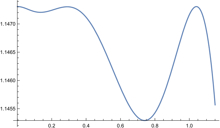
Figure 2. The function $g_{1}$ defined in (5.2) on the interval $[0,1.1]$.

5.2. Lower bound numerics

Consider the Fourier transform pairs

$$F_{n}(x)=\frac{(2n-1)!}{\pi(1+2ix)^{2n}};\qquad\widehat{F_{n}}(t)=-(\pi t)^{2n-1}\,e^{\pi t}\,{\bf 1}_{\mathbb{R}_{-}}(t),$$ (5.3)

and note that $F_{n}(x)\in\mathcal{A}_{\infty}$ for all positive integers $n$. In §2.4.2, we showed that the function $F_{1}(x)$ yields the extremal value $C(\infty)=1$. We now consider the following family of test functions, composed by dilations and translations of linear combinations of functions as in (5.3), defined in terms of their Fourier transform:

$$\widehat{F}(t)=g\left(\frac{\pi t-c}{a}\right),\text{ where }\ g(t)=\sum_{n=1}^{N}b_{n}\,t^{2n-1}\,e^{t}\,{\bf 1}_{\mathbb{R}_{-}}(t).$$ (5.4)

Here, $b_{n},c\in\mathbb{R}$ and $a>0$. Taken over this family of functions, (EP1) is an unrestricted optimization problem over $\mathbb{R}^{N+2}$ on the variables $b_{1},\ldots,b_{N},a,c$. The functional to maximize involves a numerical computation of the several integrals that appear in the formulation of (EP1) in (1.4). It is also not smooth, since the integrands involve taking $L^{1}$-norms of complex-valued functions and positive and negative parts of real-valued functions. As before, we compute the integrals in floating point arithmetic, using sufficient precision to justify the decimal digits shown in this section, in the sense that the digits that we will show remain stable after successively increasing precision. To optimize such a functional, we use the principal axis method of Brent [4], which searches for a local maximum of an unrestricted, non-smooth problem.

In Table 2, we give our lower bound for $C(A)$ for each value of $A$, together with the parameters necessary to construct the test function as defined in (5.4).

$A$	$\frac{1}{4}$	$\frac{1}{3}$	$\frac{1}{2}$	$1$	$3$
Bound	1.31706	1.27722	1.22112	1.14600	1.06082
$a$	0.856	0.727	0.587	0.1135	0.209
$c$	1.082	0.922	0.758	0.626	0.201
$b_{1}$	0.151	0.14	0.1135	$-1.562*10^{20}$	0.042
$b_{2}$	2	2	2	2	2
$b_{3}$	-0.0961	-0.0636	0.0000	$1.983*10^{21}$	0.0119
$b_{4}$	0.00233	0.00142	0.0000	$-7.316*10^{18}$	0.00495
$b_{5}$	-0.0000228	$-9.542*10^{-6}$	0.0000	$5.360*10^{17}$	-0.000592
$b_{6}$	$7.0009*10^{-8}$	$-2.224*10^{-8}$	0.0000	$1.561*10^{15}$	$1.122*10^{-6}$
$b_{7}$	$1.132*10^{-10}$	$3.962*10^{-10}$	0.0000	$-1.340*10^{13}$	$-5.946*10^{-9}$
$b_{8}$	$-6.493*10^{-13}$	$-1.0272*10^{-12}$	0.0000	$1.107*10^{11}$	$2.41*10^{-11}$
$b_{9}$	$2.053*10^{-16}$	$8.035*10^{-16}$	0.0000	$1.522*10^{8}$	$-1.688*10^{-14}$
$b_{10}$	0.0000	$-6.439*10^{-19}$	0.0000	$-1.178*10^{6}$	$-3.199*10^{-17}$
$b_{11}$	0.0000	0.0000	0.0000	$2391.83$	$1.087*10^{-19}$
$b_{12}$	0.0000	0.0000	0.0000	-0.698149	$4.339*10^{-23}$

Table 2. Lower bounds for $\mathcal{C}(A)$ for each $A$, and the parameters to define the corresponding test functions for (EP1), defined as in (5.4).

In Figures 4 and 4 we plot the functions $\widehat{F}(t)/\widehat{F}(0)$, defined as in (5.4) for $A=1$ and $A=3$ (respectively), and where we normalized by dividing by $\widehat{F}(0)$ for a better comparison between the two plots.

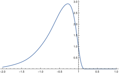
Figure 3. The function $\widehat{F}(t)/\widehat{F}(0)$ defined in (5.4) for $A=1$, with the corresponding parameters from Table 2.

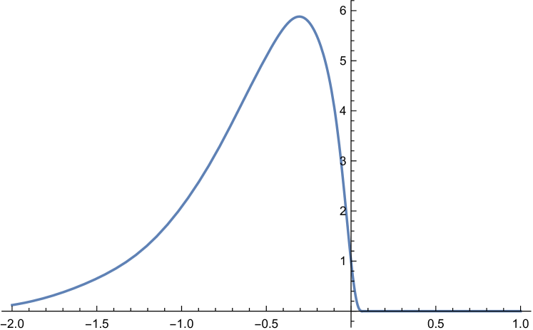
Figure 4. The function $\widehat{F}(t)/\widehat{F}(0)$ defined in (5.4) for $A=3$, with the corresponding parameters from Table 2.

Remark: Recent works have used strong computational techniques, in particular semidefinite programming, to find numerical bounds for Fourier optimization problems associated to some number theoretic quantities of interest (see, for instance, [14, 15, 31]). The fact that we must necessarily work with complex-valued functions $F\in L^{1}(\mathbb{R})$ is an important difference to the Fourier analysis frameworks in the aforementioned works (which use even, real-valued functions), and it is not clear if a similar approach with semidefinite programming may be applied in our situation.

References

- [1] N. C. Ankeny, The least quadratic non residue, Ann. of Math. (2) 55 (1952), 65–72.
- [2] E. Bach, Explicit bounds for primality testing and related problems, Math. Comp. 55 (1990), no. 191, 355–380.
- [3] E. Bach and J. Sorenson, Explicit bounds for primes in residue classes, Math. Comp. 65 (1996), no. 216, 1717–1735.
- [4] R. P. Brent, Algorithms for minimization without derivatives, Prentice-Hall Series in Automatic Computation. Prentice- Hall, Inc., Englewood Cliffs, N.J., 1973.
- [5] E. Carneiro, V. Chandee, A. Chirre, and M. B. Milinovich, On Montgomery’s pair correlation conjecture: a tale of three integrals, J. Reine Angew. Math. 786 (2022), 205–243.
- [6] E. Carneiro, V. Chandee, F. Littmann, and M. B. Milinovich, Hilbert spaces and the pair correlation of zeros of the Riemann zeta-function, J. Reine Angew. Math. 725 (2017), 143–182.
- [7] E. Carneiro, V. Chandee, and M. B. Milinovich, Bounding and on the Riemann hypothesis, Math. Ann. 356 (2013), no. 3, 939–968.
- [8] E. Carneiro and A. Chirre, Bounding on the Riemann hypothesis, Math. Proc. Cambridge Philos. Soc. 164 (2018), no. 2, 259–283.
- [9] E. Carneiro, A. Chirre, and M. B. Milinovich, Hilbert spaces and low-lying zeros of -functions, Adv. Math. 410 (2022), part B, Paper No. 108748, 48 pp.
- [10] E. Carneiro and R. Finder, On the argument of L-functions, Bull. Braz. Math. Soc. (N.S.) 46 (2015), no. 4, 601–620.
- [11] E. Carneiro, M. B. Milinovich, and A. P. Ramos, Fourier optimization and Montgomery’s pair correlation conjecture, preprint, arXiv:2310.01913.
- [12] E. Carneiro, M. B. Milinovich, and K. Soundararajan, Fourier optimization and prime gaps, Comment. Math. Helv. 94 (2019), no. 3, 533–568.
- [13] V. Chandee and K. Soundararajan, Bounding on the Riemann hypothesis, Bull. London Math. Soc. 43 (2011), no. 2, 243–250.
- [14] A. Chirre, F. Gonçalves, and D. de Laat, Pair correlation estimates for the zeros of the zeta function via semidefinite programming, Adv. Math. 361 (2020), 106926, 22.
- [15] A. Chirre, V. J. Pereira Júnior, and D. de Laat, Primes in arithmetic progressions and semidefinite programming, Math. Comp. 90 (2021), no. 331, 2235–2246.
- [16] A. Chirre and E. Quesada-Herrera, Fourier optimization and quadratic forms, Q. J. Math. 73 (2022), no. 2, 539–577.
- [17] H. Cohn and N. Elkies, New upper bounds on sphere packings. I. Ann. of Math. (2) 157 (2003), no. 2, 689–714.
- [18] H. Cohn, A. Kumar, S. D. Miller, D. Radchenko, and M. Viazovska, The sphere packing problem in dimension 24, Ann. Math. 185 (2017), 1017–1033.
- [19] H. Cohn, A. Kumar, S. D. Miller, D. Radchenko, and M. Viazovska, Universal optimality of the and Leech lattices and interpolation formulas, Ann. of Math. (2) 196 (2022), no. 3, 983–1082.
- [20] J. Freeman and S. J. Miller, Determining optimal test functions for bounding the average rank in families of -functions, SCHOLAR – a scientific celebration highlighting open lines of arithmetic research, 97–116, Contemp. Math., 655, Centre Rech. Math. Proc., Amer. Math. Soc., Providence, RI, 2015.
- [21] P. X. Gallagher, Pair correlation of zeros of the zeta function, J. Reine Angew. Math. 362 (1985), 72–86.
- [22] D. V. Gorbachev, Extremal problem for entire functions of exponential spherical type, connected with the Levenshtein bound on the sphere packing density in (Russian), Izvestiya of the Tula State University Ser. Mathematics Mechanics Informatics 6 (2000), 71–78.
- [23] D. R. Heath-Brown, Zero-free regions for Dirichlet L-functions, and the least prime in an arithmetic progression, Proc. London Math. Soc. (3) 64 (1992), no. 2, 265–338.
- [24] H. Iwaniec and E. Kowalski, Analytic Number Theory, AMS Colloquium Publications, vol. 53 (2004).
- [25] Y. Lamzouri, X. Li, and K. Soundararajan, Conditional bounds for the least quadratic non-residue and related problems, Math. Comp. 84 (2015), no. 295, 2391–2412.
- [26] Y. Lamzouri, X. Li, and K. Soundararajan, Corrigendum to “Conditional bounds for the least quadratic non-residue and related problems”, Math. Comp. 86 (2017), no. 307, 2551–2554.
- [27] H. L. Montgomery, Distribution of the zeros of the Riemann zeta function, Proceedings of the International Congress of Mathematicians (Vancouver, B. C., 1974), Vol. 1, pp 379–381. Canad. Math. Congress, Montreal, Que., 1975
- [28] H. L. Montgomery and R. C. Vaughan, Multiplicative number theory. I. Classical theory. Cambridge Studies in Advanced Mathematics, 97. Cambridge University Press, Cambridge, 2007.
- [29] H. L. Montgomery and R. C. Vaughan, The large sieve, Mathematika 20 (1973), 119–134.
- [30] H. Iwaniec, W. Luo, and P. Sarnak, Low-lying zeros of families of -functions, Publ. Math. Inst. Hautes Études Sci. 91 (2000) 55–131.
- [31] E. Quesada-Herrera, On the q-analogue of the pair correlation conjecture via Fourier optimization, Math. Comp. 91 (2022), no. 337, 2347–2365.
- [32] A. Selberg, Contributions to the theory of Dirichlet’s -functions, Skr. Norske Vid.-Akad. Oslo I 1946 (1946), no. 3, 62 pp.
- [33] K. Sono, A note on simple zeros of primitive Dirichlet -functions, Bull. Aust. Math. Soc. 93 (2016), no. 1, 19–30.
- [34] M. Viazovska, The sphere packing problem in dimension 8, Ann. Math. 185 (2017), 991–1015.
- [35] A. I. Vinogradov and Ju. V. Linnik, Hypoelliptic curves and the least prime quadratic residue, Dokl. Akad. Nauk SSSR., 168 (1966), 258–261.
- [36] T. Xylouris, On Linnik’s constant, Acta Arith. 150 (2011), 65–91.