Detecting a Gravitational-Wave Background from Null Energy Condition Violation: Prospects for Taiji

Abstract

The null energy condition (NEC) is a fundamental principle in general relativity, and its violation could leave discernible signatures in gravitational waves (GWs). A violation of the NEC during the primordial era would imprint a blue-tilted spectrum on the stochastic gravitational wave background (SGWB) at nanohertz frequencies, potentially accounting for the recently detected signal by pulsar timing arrays. Remarkably, models of NEC violation during inflation also predict a nearly scale-invariant GW spectrum in the millihertz frequency range, which could be detectable by upcoming space-based GW detectors such as Taiji. The observation of this distinctive spectrum would provide compelling evidence for new physics beyond the standard cosmological paradigm. In this study, we explore Taiji’s ability to detect an SGWB arising from NEC violation during inflation, considering various foregrounds and noise sources, including an extragalactic foreground from binary black hole mergers throughout the universe, a galactic foreground from white dwarf binaries, and the intrinsic noise of the Taiji detector. Employing comprehensive Bayesian parameter estimation techniques to analyze simulated Taiji data, we demonstrate a remarkable precision improvement of three orders of magnitude compared to the NANOGrav 15-year data set for measuring the tensor power spectrum amplitude, $P_{T,2}$, during the second inflationary stage. This substantial enhancement in measurement capabilities underscores Taiji’s potential as a powerful probe for investigating the NEC violation in the early Universe.

1 Introduction

The direct detection of gravitational waves (GWs) [1] has not only confirmed a major prediction of Einstein’s theory of general relativity but also opened a novel observational window into the universe [2, 3, 4]. While observations have primarily focused on transient GW events from the binary black hole and neutron star mergers, detected by ground-based interferometers like LIGO [5] and Virgo [6], these detections have revolutionized our understanding of compact objects and their coalescence dynamics [7, 8, 9]. However, an equally promising and more elusive target for GW detectors is the stochastic gravitational-wave background (SGWB), which carries a wealth of information about the early universe and the fundamental laws of physics.

The landscape of GW astronomy is rapidly advancing, with pulsar timing arrays (PTAs) emerging as a critical tool for probing the low-frequency GW spectrum. Recent announcements from leading PTA collaborations, including NANOGrav [10, 11], PPTA [12, 13], EPTA [14, 15], and CPTA [16], have provided compelling evidence of a stochastic signal that aligns with the Hellings-Downs spatial correlations [17] expected from an SGWB as predicted by general relativity. These findings mark a significant milestone in the detection of GWs through the timing of highly stable millisecond pulsars.

Despite these achievements, the exact origin of the observed PTA signals remains elusive [18, 19], with hypotheses spanning both astrophysical and cosmological sources. The diverse potential origins include supermassive black hole binaries [20, 21, 22, 23, 24], as well as more exotic phenomena such as scalar-induced GWs [25, 26, 27, 28, 29, 30, 31, 32, 33, 34, 35, 36, 37, 38] that could be linked to primordial black hole formation [39, 40, 41, 42, 43, 44, 45], cosmic phase transitions [46, 47, 48, 49, 50, 51, 52, 53, 54], domain walls [55, 56, 57], and cosmic strings [58, 59, 60, 61]. Another exciting possibility is that the detected signal is the SGWB from the violation of the null energy condition (NEC) in the early universe [62].

The NEC is a fundamental principle in general relativity, asserting that the contraction of any null vector with the energy-momentum tensor yields a non-negative value. However, NEC violation has been hypothesized to explain various early Universe phenomena, such as inflation and primordial black hole formation [63, 64, 65, 66, 67, 68, 69, 70, 71]; see the review by [72]. Recent developments in modified gravity theories, particularly those beyond Horndeski models [73, 74, 75, 76, 77], have demonstrated the theoretical possibility of stable NEC violations, overcoming pathological instabilities. The violation of the NEC has a significant impact on the generation of primordial GWs in the early Universe, leading to an amplification of the primordial tensor power spectrum [78, 79]. This amplification is characterized by a blue tilt in the tensor power spectrum, signifying enhanced production of high-frequency GWs. Consequently, the SGWB is expected to exhibit a distinctive pattern that reflects the NEC-violating phase. The detection of this characteristic signature in the SGWB would provide strong evidence for NEC-violating physics and shed light on the nature of gravity at high energies.

Investigating NEC violation through its effect on the SGWB presents a novel approach to probing early Universe physics, complementing other cosmological observations. By comparing the theoretical predictions of NEC-violating models with observational SGWB constraints, valuable insights can be gained into the fundamental laws governing the Universe’s earliest stages, enabling the exploration of new physics beyond the standard cosmological paradigm. Remarkably, models of NEC violation during inflation also predict a nearly scale-invariant GW spectrum in the millihertz frequency range, which could be detectable by upcoming space-based GW detectors such as Taiji. The Taiji program [80], China’s space-based GW observatory, is poised to contribute significantly to this frontier of physics. With its planned launch in the near future, Taiji will surpass the sensitivity of current ground-based detectors at low frequencies and thus holds the potential to detect the subtle signals of an SGWB. Prospects for Taiji are bolstered by its ability to operate in a frequency band that complements LIGO, Virgo, and PTA, providing a broad observational baseline to search for GW signals.

In this paper, we investigate the SGWB produced by NEC violation during inflation and constrain the model parameters using the NANOGrav 15-year data set. We then analyze simulated Taiji data and apply parameter estimation techniques to quantify the uncertainties in determining the model parameters. This analysis provides valuable insights into the precision and accuracy of parameter estimation for the SGWB produced by NEC violation during inflation, as well as the detection capabilities of Taiji. The paper is structured as follows. In Sec. 2, we offer a brief review of the SGWB produced by the NEC violation during inflation and the constraints on the model parameters obtained from the NANOGrav 15-year data set. Sec. 3 introduces the various components of the model used in the simulation and parameter estimation, including the Taiji noise model, the foreground from double white dwarfs (DWDs), and the extragalactic compact binary (ECB) foreground. The methodology for simulating Taiji data and inferring model parameters is described in Sec. 4. Finally, we summarize our findings and provide concluding remarks in Sec. 5.

2 SGWB from NEC violation during inflation

The intermediate NEC violation during inflation is a captivating scenario that has been proposed to explain the distinctive features of the primordial GW background. In this section, we will delve into the intricate details of this model, as outlined by [62].

The Universe is assumed to begin with an initial phase of slow-roll inflation, characterized by a Hubble parameter $H=H_{\text{inf1}}$. This stage sets the foundation for the subsequent evolution of the Universe. As the inflationary epoch progresses, a fascinating transition occurs: the Universe enters a second phase of slow-roll inflation, marked by a significantly larger Hubble parameter, $H=H_{\text{inf2}}$. This transition is not instantaneous; instead, it is punctuated by an intermediate stage of NEC violation, which serves as a bridge between the two slow-roll inflationary phases. Throughout this intricate evolution, a remarkable phenomenon takes place: the comoving Hubble horizon,$a^{-1}H^{-1}$, undergoes a continuous decrease. This reduction in the comoving Hubble horizon has profound implications for the behaviour of perturbation modes. As the Universe experiences accelerated expansion during inflation, perturbation modes gradually exit the horizon, crossing the threshold from the sub-horizon to the super-horizon regime. These modes remain in the super-horizon state until they re-enter the horizon during the ensuing radiation-dominated or matter-dominated era.

The power spectra of perturbation modes exiting the horizon during the first ($k<k_{1}$) and second ($k>k_{2}$) stages of slow-roll inflation exhibit a remarkable property: they are nearly scale-invariant. This scale-invariance is a crucial feature, as it aligns with the observations of the cosmic microwave background temperature anisotropies. However, a striking difference emerges between the two stages. The power spectrum amplitude of modes exiting during the second stage is significantly larger than that of the modes exiting during the first stage. This amplification in the power spectrum amplitude is a hallmark of the intermediate NEC violation scenario. The scale-invariance of the tensor power spectrum at large scales has important consequences for the tensor-to-scalar ratio $r$ and the slow-roll parameter in canonical single-field slow-roll inflation. The non-suppressed nature of these quantities ensures their compatibility with observational constraints. Moreover, at small scales, the scale-invariance of both scalar and tensor power spectra plays a crucial role in maintaining the validity of perturbation theory at higher frequencies. By preventing the power spectra from growing to $\mathcal{O}(1)$, the scale-invariance ensures that the perturbation approach remains valid and reliable.

The primordial tensor power spectrum $P_{T}$ is a fundamental quantity that encapsulates the essential features of the SGWB produced during the early Universe. In this work, we adopt the parametrization proposed by [62], which elegantly captures the key characteristics of the power spectrum in the presence of an intermediate NEC violation during inflation:

$$P_{T}=P_{T,1}+\frac{\pi}{4}(2-n_{T})\frac{k}{k_{2}}|g(k)|^{2}P_{T,2},$$ (2.1)

where $P_{T,1}$ and $P_{T,2}$ represent the power spectrum amplitudes during the first and second slow-roll inflationary stages, and the auxiliary function $g(k)$ is expressed as

$$g(k)=H_{\frac{3-n_{T}}{2}}^{(1)}\left[\frac{2-n_{T}}{2}\frac{k}{k_{2}}\right]\sin\frac{k}{k_{2}}+H_{\frac{1-n_{T}}{2}}^{(1)}\left[\frac{2-n_{T}}{2}\frac{k}{k_{2}}\right]\left(\cos\frac{k}{k_{2}}-\frac{k_{2}}{k}\sin\frac{k}{k_{2}}\right)~{}.\textbf{}$$ (2.2)

Here, $n_{T}$ denotes the tensor spectral index during the NEC-violating stage and $H_{\nu}^{(1)}$ is the Hankel function of the first kind. In the limit of $k\ll k_{1}$, the primordial tensor power spectrum $P_{T}$ is approximately equal to $P_{T,1}$, as the second term in Eq. (2.1) becomes negligible compared to $P_{T,1}$. On the other hand, for $k\gg k_{1}$, the second term in Eq. (2.1) becomes dominant, ensuring that the features around $k\simeq k_{2}$ are well captured. Although this formulation may sacrifice some accuracy around the first transition scale $k\simeq k_{1}$, the impact of this compromise on our interests is minimal. The primordial tensor power spectrum $P_{T}$ can be converted to the GW energy spectrum using the relation given by [81]:

$$\Omega_{\rm{GW}} =\frac{k^{2}}{12H_{0}^{2}}\left[\frac{3\Omega_{m}j_{l}(k\tau_{0})}{k\tau_{0}}\sqrt{1.0+1.36\frac{k}{k_{\text{eq}}}+2.50\left(\frac{k}{k_{\text{eq}}}\right)^{2}}\right]^{2}P_{T}$$ (2.3)

$$\simeq\frac{1}{24}\left(\frac{k}{H_{0}}\right)^{2}\left[\frac{3\Omega_{m}}{(k\tau_{0})^{2}}\sqrt{1.0+1.36\frac{k}{k_{\text{eq}}}+2.50\left(\frac{k}{k_{\text{eq}}}\right)^{2}}\right]^{2}P_{T}$$

where $\tau_{0}=1.41\times 10^{4}$ Mpc, $H_{0}=67.4\,{\rm km/s/Mpc}$ is the Hubble constant [82], $k_{\text{eq}}=0.073\,\Omega_{\text{m}}h^{2}$ Mpc^-1 is the wavenumber at matter-radiation equality, $\Omega_{\rm m}$ is the density fraction of matter today, and the wavenumber $k$ is related to the frequency $f$ by $k=2\pi f$. This relation allows us to translate the primordial tensor power spectrum, which is a function of wavenumber $k$, into the observable GW energy spectrum $\Omega_{\rm{GW}}$. The GW energy spectrum represents the fraction of the critical energy density of the Universe that is contained in GWs at a given frequency. As previously discussed, our focus lies on the case where $k_{1}\ll k$. In this regime, the first term in Eq. (2.1) becomes significantly smaller than the second term, allowing us to safely neglect $P_{T,1}$. This simplification leads to a more manageable parametrization of the theoretical spectrum, which is now fully characterized by three parameters: ${P_{T,2},\ n_{T},\ f_{c}}$. The transition frequency $f_{c}$ is related to the characteristic scale $k_{2}$ by the relation $f_{c}\equiv 2\pi k_{2}$.

Figure 1: Parameter estimation results derived from the NANOGrav 15-year data set, with the red dot indicating the maximum-likelihood values used as the basis for the Taiji data injections. Here, the contours in 2D plots correspond to $1\sigma$, $2\sigma$, and $3\sigma$ confidence levels in the parameter space.

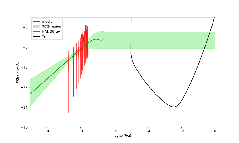
Figure 2: Posterior predictive distribution of the energy density spectrum resulting from NEC violation during inflation (green color), alongside the free spectrum derived from the NANOGrav 15-year data set (red color) and the power-law integrated sensitivity curves for Taiji (black dashed line).

The recently detected PTA signal can potentially be explained by the SGWB produced by primordial NEC violation during inflation [62]. To constrain the model parameters using the NANOGrav 15-year data set, we perform a Bayesian inference following the methodology outlined in [23, 25, 83, 28, 29], taking into account the Hellings-Downs correlations. The resulting posterior distributions, shown in Fig. 1, yield the following parameter estimates: $P_{T,2}=0.14^{+0.68}_{-0.12}$, $f_{c}=4.2^{+2.0}_{-3.2}\times 10^{-8}\,{\mathrm{Hz}}$, and $n_{T}=1.66^{+0.31}_{-0.68}$. These posterior distributions are broadly consistent with those reported in [62]. Fig. 2 illustrates the posterior predictive distribution for the GW energy density, along with the power-law integrated sensitivity curves of the Taiji detector. The wide frequency range covered by the energy density spectrum suggests that the SGWB generated by NEC violation during inflation could be detectable by Taiji. Motivated by these findings, we will focus on examining the detection capability of the Taiji detector for this specific SGWB signal in the following analysis.

3 Model components

In this section, we present the key components of our model for analyzing the sensitivity of the Taiji mission to SGWBs. We consider the instrumental noise characteristics of the Taiji detector, as well as two important astrophysical foregrounds: the DWD foreground and the ECB foreground.

3.1 Taiji noise model

The triangular geometry of the Taiji detector enables the combination of interferometric phase differences using the time delay interferometry (TDI) techniques to suppress laser frequency noise [84, 85]. This process results in the creation of three independent GW measurement channels: the $X,Y,Z$ TDI channels [86]. Accurately characterizing the noise properties in the Taiji mission is a complex technical challenge, and a detailed analysis of the noise intricacies is beyond the scope of this work. For the purposes of this study, we make several simplifying assumptions regarding the SGWB signal and the instrument noise. We assume that the SGWB signal in the $X,Y,Z$ channels is stationary and uncorrelated with the Taiji instrument noise. Additionally, we model the instrument noise as consisting of test mass acceleration noise and optical path length fluctuation noise, which are assumed to be identical in each spacecraft. Furthermore, we consider the Taiji instruments’ arm lengths to be equal, forming an equilateral triangle with arm lengths $L_{1}=L_{2}=L_{3}=L=3\times 10^{9}\,\mathrm{m}$. Under these assumptions, the response functions and cross-spectra of the $X,Y,Z$ channel combinations are found to be identical [87]. These simplifications allow us to focus on the key aspects of the Taiji detector’s performance in detecting the SGWB signal while maintaining a tractable analysis. By assuming stationarity and the absence of correlation between the SGWB signal and the instrument noise, we can treat the two components independently and simplify the statistical analysis. The assumption of identical noise properties in each spacecraft and equal arm lengths further reduces the complexity of the problem, enabling us to derive concise expressions for the response functions and cross-spectra of the TDI channels. While these assumptions may not capture the full complexity of the Taiji mission, they provide a solid foundation for understanding the detector’s sensitivity to the SGWB and serve as a starting point for more detailed analyses in the future.

The noise components of the Taiji instrument can be effectively described by two distinct functions. The high-frequency noise, originating from the optical metrology system, is characterized by the power spectral density (PSD) as [88]

$$P_{\mathrm{oms}}(f)=P^{2}\times 10^{-24}\frac{1}{\mathrm{Hz}}\left[1+\left(\frac{2\,\mathrm{mHz}}{f}\right)^{4}\right]\left(\frac{2\pi f}{c}\mathrm{m}\right)^{2},$$ (3.1)

where $f$ denotes the frequency, $c$ represents the speed of light, and $P=8$ [89]. The low-frequency noise, associated with test mass acceleration, is captured by the PSD [88]

$$P_{\mathrm{acc}}(f)=A^{2}\times 10^{-30}\frac{1}{\mathrm{Hz}}\left[1+\left(\frac{0.4\,\mathrm{mHz}}{f}\right)^{2}\right]\left[1+\left(\frac{f}{8\,\mathrm{mHz}}\right)^{4}\right]\left(\frac{1}{2\pi fc}\frac{\mathrm{m}}{\mathrm{s}^{2}}\right)^{2},$$ (3.2)

where $A=3$ [89]. The total PSD for the noise auto-correlation is given by

$$N_{aa}(f,A,P)=16\sin^{2}\left(\frac{f}{f_{*}}\right)\left\{\left[3+\cos\left(\frac{2f}{f_{*}}\right)\right]P_{\mathrm{acc}}(f,A)+P_{\mathrm{oms}}(f,P)\right\},$$ (3.3)

where $f_{*}=c/(2\pi L)$ is a characteristic frequency determined by the arm length $L$. The noise cross-spectra are expressed as

$$N_{ab}(f,A,P)=-8\sin^{2}\left(\frac{f}{f_{*}}\right)\cos\left(\frac{f}{f_{*}}\right)\left[4P_{\mathrm{acc}}(f,A)+P_{\mathrm{oms}}(f,P)\right],$$ (3.4)

where $a,b\in\{\mathrm{X},\mathrm{Y},\mathrm{Z}\}$ and $a\neq b$. Note that the noise covariance matrix is real under these assumptions.

To simplify the analysis, we can utilize linear combinations of the channels. For the space-borne GW instrument, three particular channels are frequently employed: the noise “orthogonal” channels $A$ and $E$, and the “null” channel $T$. These channels are defined as follows:

$$\left\{\begin{array}[]{l}A=\frac{1}{\sqrt{2}}(Z-X),\\ E=\frac{1}{\sqrt{6}}(X-2Y+Z),\\ T=\frac{1}{\sqrt{3}}(X+Y+Z).\end{array}\right.$$ (3.5)

These combinations offer the advantage of noise orthogonality and reduced sensitivity to GWs in the null channel $T$. In the AET basis, the noise spectra can be expressed as

$$N_{\mathrm{A}} = N_{\mathrm{E}}=N_{\mathrm{XX}}-N_{\mathrm{XY}},$$ (3.6)

$$N_{\mathrm{T}} = N_{\mathrm{XX}}+2N_{\mathrm{XY}}.$$ (3.7)

By substituting the noise auto- and cross-spectra from Eq. (3.3) and Eq. (3.4) into these expressions, we obtain the following results for the noise spectra in the AE and T channels:

$$N_{\mathrm{A,E}}=8\sin^{2}\left(\frac{f}{f_{*}}\right)\left\{4\left[1+\cos\left(\frac{f}{f_{*}}\right)+\cos^{2}\left(\frac{f}{f_{*}}\right)\right]P_{\mathrm{acc}}+\left[2+\cos\left(\frac{f}{f_{*}}\right)\right]P_{\mathrm{oms}}\right\},$$ (3.8)

and

$$N_{\mathrm{T}}=16\sin^{2}\left(\frac{f}{f_{*}}\right)\left\{2\left[1-\cos\left(\frac{f}{f_{*}}\right)\right]^{2}P_{\mathrm{acc}}+\left[1-\cos\left(\frac{f}{f_{*}}\right)\right]P_{\mathrm{oms}}\right\}.$$ (3.9)

The use of the AET basis and these noise spectra expressions greatly simplifies the analysis of the Taiji instrument’s sensitivity to GWs, as it allows for a clear separation of the noise contributions and a straightforward comparison of the noise levels in the different channels.

To facilitate our analysis, we define the equivalent energy spectral density as

$$\Omega_{\alpha}(f)=S_{\alpha}(f)\frac{4\pi^{2}f^{3}}{3H_{0}^{2}},$$ (3.10)

where $\alpha\in\{\mathrm{A,E,T}\}$ denotes the different channel combinations, and $S_{\alpha}$ represents the corresponding noise spectral densities. These noise spectral densities can be expressed as

$$S_{\mathrm{A}}(f) = S_{\mathrm{E}}(f)=\frac{N_{\mathrm{A}}(f)}{\mathcal{R}_{\mathrm{A,E}}(f)},$$ (3.11)

$$S_{\mathrm{T}}(f) = \frac{N_{\mathrm{T}}(f)}{\mathcal{R}_{\mathrm{T}}(f)},$$ (3.12)

where $\mathcal{R}\alpha$ denotes the response functions for each channel. Approximate expressions for these response functions have been provided in [90], which take the form

$$\mathcal{R}_{\mathrm{A}}^{\mathrm{Fit}}(f) = \mathcal{R}_{\mathrm{E}}^{\mathrm{Fit}}(f)=\frac{9}{20}|W(f)|^{2}\left[1+\left(\frac{f}{4f_{*}/3}\right)^{2}\right]^{-1},$$ (3.13)

$$\mathcal{R}_{\mathrm{T}}^{\mathrm{Fit}} \simeq \frac{1}{4032}\left(\frac{f}{f_{*}}\right)^{6}|W(f)|^{2}\left[1+\frac{5}{16128}\left(\frac{f}{f_{*}}\right)^{8}\right]^{-1},$$ (3.14)

where $W(f)=1-e^{-2if/f_{*}}$. While these approximate expressions can be useful, in this study, we employ the more accurate analytical expressions for the response functions that were recently derived in [91]. These analytical expressions provide a more precise description of the detector’s response and are essential for the accurate characterization of the GW signal.

3.2 Double white dwarf foreground

Astrophysical population models [92, 93] predict the existence of tens of millions of DWD binaries within our Milky Way galaxy. These DWD binaries are expected to emit GWs simultaneously within a frequency range spanning from $10^{-5}\,\mathrm{Hz}$ to $0.1\,\mathrm{Hz}$ [94]. While a small fraction of these DWD binaries are individually resolvable, the vast majority remain unresolved and collectively contribute to a stochastic “galactic foreground” or “confusion noise” for the Taiji mission [95]. The DWD foreground can be approximated by a polynomial function $S_{c}(f)$ in the logarithmic scale as [95]

$$S_{\mathrm{DWD}}(f)=\exp\left(\sum_{i=0}^{5}a_{i}\left(\log\left(\frac{f}{\mathrm{mHz}}\right)\right)^{i}\right)\mathrm{Hz}^{-1}.$$ (3.15)

This approximation is valid for the frequency range $0.1\,\mathrm{mHz}<f<10\,\mathrm{mHz}$. The values of the parameters $a_{i}$ for a $4$-year observation are $a_{0}=-85.5448$, $a_{1}=-3.23671$, $a_{2}=-1.64187$, $a_{3}=-1.14711$, $a_{4}=0.0325887$, $a_{5}=0.187854$. The corresponding dimensionless energy spectral density is given by

$$\Omega_{\mathrm{DWD}}(f)=S_{\mathrm{DWD}}(f)\frac{4\pi^{2}f^{3}}{3H_{0}^{2}}.$$ (3.16)

In this work, we employ a broken power law to model the dimensionless energy spectral density $\Omega_{\mathrm{DWD}}$ of the DWD foreground. The expression for $\Omega_{\mathrm{DWD}}(f)$ is given by

$$\Omega_{\mathrm{DWD}}(f)=\frac{A_{1}\left(f/f_{*}\right)^{\alpha_{1}}}{1+A_{2}\left(f/f_{*}\right)^{\alpha_{2}}},$$ (3.17)

with the following parameter values: $A_{1}=3.98\times 10^{-16}$, $A_{2}=4.79\times 10^{-7}$, $\alpha_{1}=-5.7$, and $\alpha_{2}=-6.2$ [96]. The broken power-law spectral shape of the DWD foreground arises from the physical constraint imposed by the finite radii of the two white dwarfs in each binary system. As the frequency increases, the number of DWDs capable of emitting at those frequencies decreases, leading to a change in spectral behaviour.

3.3 Extragalactic compact binary foreground

The existence of a background originating from compact binaries, comprising black holes and neutron stars, in distant galaxies is predicted by current models [97]. Nevertheless, ground-based GW observatories have not yet succeeded in detecting this ECB foreground. In this study, we model the energy spectral density of the ECB foreground using a power-law approximation:

$$\Omega_{\mathrm{ECB}}(f)=A_{\mathrm{ECB}}\left(\frac{f}{f_{\mathrm{ref}}}\right)^{\alpha_{\mathrm{ECB}}},$$ (3.18)

where $f_{\mathrm{ref}}=25\mathrm{Hz}$ is the reference frequency, and $\alpha_{\mathrm{ECB}}=\frac{2}{3}$ represents the power-law index. The amplitude $A_{\mathrm{ECB}}$ is estimated to be $1.8\times 10^{-9}$, based on the findings presented in [97]. The inclusion of the ECB foreground is crucial for accurately assessing the mission’s ability to detect and characterize other sources of SGWBs, such as those originating from the early Universe or more exotic phenomena. As the sensitivity of GW detectors continues to improve, the detection and precise characterization of the ECB foreground will become increasingly important for advancing our understanding of the population and evolution of compact binary systems throughout the cosmos.

4 Methodology

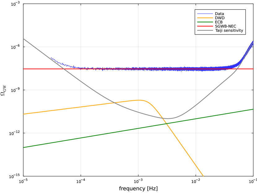
Figure 3: The simulated A-channel data (blue) for Taiji in the frequency domain. The DWD foreground (orange), ECB foreground (green), and SGWB produced by NEC violation (red) are also shown. Additionally, the Taiji sensitivity curve is displayed in terms of the dimensionless energy spectral density $\Omega_{\mathrm{GW}}(f)$.

In this study, we simulate the Taiji data, closely adhering to the procedures outlined in Refs. [98, 87]. We consider a scenario where data is collected over a full mission duration of $4$ years, with an estimated efficiency of $75\%$, resulting in an effective observation time of $3$ years. The TDI data is segmented into approximately $N_{\mathrm{c}}=94$ chunks, each spanning $11.5$ days [98, 87]. The Taiji mission’s frequency range of interest extends from $3\times 10^{-5}\,\mathrm{Hz}$ to $5\times 10^{-1}\,\mathrm{Hz}$, with a frequency resolution of approximately $10^{-6}\,\mathrm{Hz}$. This results in a total of roughly $5\times 10^{7}$ data points for the entire simulation.

To analyze the data stream, we perform a Fourier transform, considering only positive frequencies due to the real nature of the time stream. The time data stream can be expressed as

$$d(t)=\sum_{f=f_{\min}}^{f_{\max}}\left[d(f)e^{-2\pi ift}+d^{*}(f)e^{2\pi ift}\right].$$ (4.1)

where $d(f)$ represents the Fourier amplitudes at frequency $f$, and $d^{*}(f)$ denotes the complex conjugate of $d(f)$. Assuming the SGWB and the noise are both stationary, namely $\langle d(t)d(t^{\prime}\rangle=f(t-t^{\prime})$ and $\langle d(t)\rangle=0$, the ensemble averages of the Fourier coefficients satisfy

$$\left\langle d(f)d\left(f^{\prime}\right)\right\rangle=0\quad\text{ and }\quad\left\langle d(f)d^{*}\left(f^{\prime}\right)\right\rangle=D(f)\delta_{ff^{\prime}},$$ (4.2)

indicating that the Fourier coefficients at different frequencies are uncorrelated, and the correlation strength at the same frequency is determined by the PSD, $D(f)$.

Parameter	Prior	Injected value	Recovered value
$A$	${\mathcal{U}}(2.95,3.05)$	$3$	$2.997^{+0.013}_{-0.013}$
$P$	${\mathcal{U}}(7.99,8.01)$	$8$	$8.000^{+0.002}_{-0.002}$
$\log_{10}A_{1}$	${\mathcal{U}}(-17,-14)$	$-15.4$	$-15.11^{+0.98}_{-1.28}$
$\alpha_{1}$	${\mathcal{U}}(-7,-4)$	$-5.7$	$-5.50^{+1.12}_{-1.27}$
$\log_{10}A_{2}$	${\mathcal{U}}(-8,-5)$	$-6.32$	$-6.96^{+1.59}_{-0.95}$
$\alpha_{2}$	${\mathcal{U}}(-9,-5)$	$-6.2$	$-6.60^{+1.20}_{-0.85}$
$\log_{10}A_{\mathrm{ECB}}$	${\mathcal{U}}(-10,-7)$	$-8.74$	$-8.38^{+0.81}_{-1.02}$
$\alpha_{\mathrm{ECB}}$	${\mathcal{U}}(0.2,1)$	$2/3$	$0.67^{+0.29}_{-0.39}$
$\log_{10}P_{T,2}$	${\mathcal{U}}(-1.52,-1.148)$	$-1.15$	$-1.1500^{+0.0005}_{-0.0007}$
$\log_{10}(f_{c}/\mathrm{Hz})$	${\mathcal{U}}(-9,-6)$	$-7.55$	$-7.51^{+1.38}_{-1.34}$
$n_{T}$	${\mathcal{U}}(1,2)$	$1.9$	$1.51^{+0.45}_{-0.46}$

Table 1: Summary of the model parameters and their associated priors employed in the Bayesian inference analysis. The injected values used in the simulation are provided, along with the recovered values obtained from the parameter estimation. The recovered values are presented as the median and $90\%$ equal-tail credible intervals. The notation ${\mathcal{U}}$ represents the uniform distribution.

To simulate a signal, we employ Gaussian distributions to generate random variables that correspond to the real and imaginary components of the Fourier coefficients. These variables are drawn from distributions with a variance of $D(f)/2$. By modelling both the signal and noise as Gaussian processes, we assert that their statistical properties can be completely described by their respective power spectra, denoted by $\Omega_{\mathrm{GW}}(f)$ for the GW signal and $\Omega_{\mathrm{A,E,T}}(f)$ for the detector noise in different channels. Specifically, at each discrete frequency $f_{i}$, we compute the signal power, $S_{i}$, and noise power, $N_{i}$, as

$$S_{i} = \left|\frac{G_{i1}\left(0,\sqrt{\Omega_{\mathrm{GW}}\left(f_{i}\right)}\right)+iG_{i2}\left(0,\sqrt{\Omega_{\mathrm{GW}}\left(f_{i}\right)}\right)}{\sqrt{2}}\right|^{2},$$ (4.3)

$$N_{i} = \left|\frac{G_{i3}\left(0,\sqrt{\Omega_{\mathrm{A,E,T}}\left(f_{i}\right)}\right)+iG_{i4}\left(0,\sqrt{\Omega_{\mathrm{A,E,T}}\left(f_{i}\right)}\right)}{\sqrt{2}}\right|^{2}.$$ (4.4)

Here, $G_{i1}(M,\sigma),\ldots,G_{i4}(M,\sigma)$ represent Gaussian-distributed real numbers with mean $M$ and standard deviation $\sigma$. These are the stochastic realizations of the real and imaginary parts of the Fourier coefficients for both signal and noise. The total power at each frequency, $D_{i}$, is obtained by summing the corresponding signal and noise powers, which we assume to be independent:

$$D_{i}=S_{i}+N_{i}.$$ (4.5)

For each frequency bin indexed by $i$, we generate a set of $N_{\mathrm{c}}$ data points, ${D_{i1},D_{i2},\ldots,D_{iN_{\mathrm{c}}}}$, and compute their mean, $\bar{D}_{i}$. The simulated data, depicted in Fig. 3, is generated using parameter values listed in Table 1.

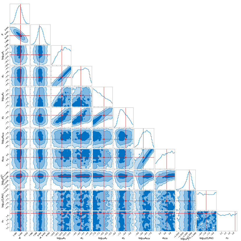
Figure 4: Posterior distributions of the model parameters for the NEC violation model, as inferred by the Taiji detector. The red points indicate the injected values for each parameter, serving as a reference for evaluating the accuracy of the parameter estimation. The contours represent the $1\sigma$, $2\sigma$, and $3\sigma$ confidence levels in the two-dimensional parameter space.

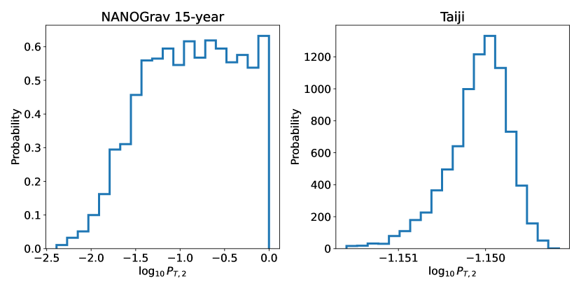
Figure 5: Comparison of the posterior distributions for the tensor power spectrum amplitude during the second inflationary stage, $P_{T,2}$, as derived from the NANOGrav 15-year data set (left panel) and the simulated Taiji mission data (right panel). The plot highlights the significant improvement in the precision of the $P_{T,2}$ measurement achieved by Taiji, with a substantially narrower posterior distribution compared to that obtained from the NANOGrav data.

To streamline the computational demands associated with high-frequency data, we employ a rebinning strategy, termed “coarse graining”, for frequencies from $f=10^{-3}\,\mathrm{Hz}$ to $f_{\max}=0.5\,\mathrm{Hz}$. The rebinning process consolidates the frequency range into $1000$ equally spaced logarithmic intervals. Frequencies in the lower spectrum, specifically from $f_{\min}=3\times 10^{-5}\,\mathrm{Hz}$ to $f=10^{-3}\,\mathrm{Hz}$, are preserved in their original form. The modified data set thus comprises $1971$ bins per segment, optimizing computational efficiency without compromising data integrity. The rebinned data within this specified frequency domain are redefined as

$$f_{k} \equiv \sum_{j\in\operatorname{bin}k}w_{j}f_{j},$$ (4.6)

$$\bar{D}_{k} \equiv \sum_{j\in\operatorname{bin}k}w_{j}\bar{D}_{j},$$ (4.7)

where $w_{j}$ are the weighting factors given by

$$w_{j}=\frac{\mathcal{D}^{\mathrm{th}}(f_{j},\vec{\theta},\vec{n})^{-1}}{\sum_{l\in\mathrm{bin}k}\mathcal{D}^{\mathrm{th}}(f_{l},\vec{\theta},\vec{n})^{-1}},$$ (4.8)

for each frequency $j$ within the aggregated interval $k$. The theoretical data model, $\mathcal{D}^{\mathrm{th}}(f,\vec{\theta},\vec{n})$, is defined by the sum of the GW spectrum, $\Omega_{\mathrm{GW}}(f,\vec{\theta})$, and detector noise, $\Omega_{\alpha}(f,\vec{n})$. Here, $\vec{n}=\{A,P\}$ represents the noise parameters, while the signal parameters are encapsulated by $\vec{\theta}=\{A_{1},\alpha_{1},A_{2},\alpha_{2},A_{\mathrm{ECB}},\alpha_{\mathrm{ECB}},n_{T},f_{c},P_{T,2}\}$. For practical analysis, we use the AET basis, which simplifies the covariance matrix to a diagonal form, facilitating more straightforward computations.

The likelihood function is computed as a composition of the Gaussian part and the log-normal part [87]. The log-likelihood combination is mathematically represented as

$$\ln\mathcal{L}=\frac{1}{3}\ln\mathcal{L}_{\mathrm{G}}+\frac{2}{3}\ln\mathcal{L}_{\mathrm{LN}}.$$ (4.9)

The Gaussian component of the likelihood, $\ln\mathcal{L}_{\mathrm{G}}$, which scrutinizes the residuals between the theoretical model and observed data, is given by

$$\ln\mathcal{L}_{\mathrm{G}}(D|\vec{\theta},\vec{n})=-\frac{N_{\mathrm{c}}}{2}\sum_{\alpha}\sum_{k}n_{\alpha}^{(k)}\left[\frac{\mathcal{D}_{\alpha}^{\mathrm{th}}\left(f_{\alpha}^{(k)},\vec{\theta},\vec{n}\right)-\mathcal{D}_{\alpha}^{(k)}}{\mathcal{D}_{\alpha}^{\mathrm{th}}\left(f_{\alpha}^{(k)},\vec{\theta},\vec{n}\right)}\right]^{2},$$ (4.10)

where the sums iterate over the AET detector channels, denoted by $\alpha$, and the frequency bins, indexed by $k$. The log-normal component, $\ln\mathcal{L}_{\mathrm{LN}}$, assesses the logarithmic deviations and is formalized as

$$\ln\mathcal{L}_{\mathrm{LN}}(D|\vec{\theta},\vec{n})=-\frac{N_{\mathrm{c}}}{2}\sum_{\alpha}\sum_{k}n_{\alpha}^{(k)}\ln^{2}\left[\frac{\mathcal{D}_{\alpha}^{\mathrm{th}}\left(f_{\alpha}^{(k)},\vec{\theta},\vec{n}\right)}{\mathcal{D}_{\alpha}^{(k)}}\right].$$ (4.11)

5 Result and discussion

We employ the dynesty [99] sampler, accessed through the Bilby package [100, 101], to thoroughly investigate the parameter space. Table 1 provides a comprehensive summary of the model parameters and their corresponding priors. Fig. 4 presents the posterior distributions for the parameters, obtained using data from the Taiji detector. The injected values, denoted in red, are overlaid on these distributions, showing that the parameters can be well recovered within a $2\sigma$ confidence interval. For ease of comparison, the median values and $90\%$ credible intervals are concisely tabulated in Table 1. Our analysis reveals that the noise parameters, denoted by $A$ and $P$, can be precisely determined with relative uncertainties of $0.4\%$ and $0.03\%$, respectively. In contrast, the parameters associated with the ECB and the DWD foregrounds exhibit larger uncertainties due to their more subtle signatures compared to the prominent SGWB from NEC violation. Remarkably, the tensor power spectrum amplitude during the second inflationary stage can be determined with an impressive relative uncertainty of $0.16\%$ with a result of $P_{T,2}=7.079^{+0.007}_{-0.012}\times 10^{-2}$. This level of precision represents a substantial improvement, more than a factor of $5000$, compared to what was achievable with the NANOGrav 15-year data. This highlights the exceptional sensitivity of the Taiji detector in refining the measurements of these crucial parameters. To effectively illustrate the progress made, we directly compare the posterior distributions obtained from the NANOGrav 15-year data set with those derived using the Taiji detector, as depicted in Fig. 5. This side-by-side comparison demonstrates the remarkable enhancements in parameter estimation achieved with Taiji, emphasizing its potential to revolutionize our understanding of NEC violation.

In this paper, we have explored the potential of the Taiji space-based GW detector to detect an SGWB originating from the violation of the NEC during inflation. We posited that the stochastic signal observed by PTAs, such as NANOGrav, stems from NEC violation during the inflationary epoch and leveraged the NANOGrav 15-year data set to constrain the model parameters. By conducting parameter estimation on simulated Taiji data, we quantified the uncertainties in determining the model parameters associated with the GW signal from NEC violation during inflation. Our results demonstrate a remarkable improvement in precision compared to the NANOGrav 15-year data set, surpassing it by more than three orders of magnitude. This significant enhancement highlights the superior measurement capabilities of the Taiji detector. Consequently, space-based GW detectors like Taiji will play a pivotal role in verifying the stochastic signal detected by PTAs and serve as invaluable tools for further validation of NEC violation signatures. Moreover, our study underscores the importance of accurately characterizing various components of the model [102, 96], including the Taiji noise model and foreground contributions from DWDs and ECBs.

In conclusion, the prospects for Taiji to detect an SGWB from NEC violation during inflation appear promising, and our study provides valuable insights into the parameter estimation and detection capabilities of Taiji for NEC violation during inflation. Future observations and analyses from Taiji and other space-based GW detectors will continue to illuminate the origin and properties of the SGWB, contributing to our understanding of the early Universe and fundamental physics.

References

- [1] LIGO Scientific, Virgo collaboration, Observation of Gravitational Waves from a Binary Black Hole Merger, Phys. Rev. Lett. 116 (2016) 061102 [1602.03837].
- [2] LIGO Scientific, Virgo collaboration, Tests of General Relativity with the Binary Black Hole Signals from the LIGO-Virgo Catalog GWTC-1, Phys. Rev. D 100 (2019) 104036 [1903.04467].
- [3] LIGO Scientific, Virgo collaboration, Tests of general relativity with binary black holes from the second LIGO-Virgo gravitational-wave transient catalog, Phys. Rev. D 103 (2021) 122002 [2010.14529].
- [4] LIGO Scientific, VIRGO, KAGRA collaboration, Tests of General Relativity with GWTC-3, 2112.06861.
- [5] LIGO Scientific collaboration, Advanced LIGO, Class. Quant. Grav. 32 (2015) 074001 [1411.4547].
- [6] VIRGO collaboration, Advanced Virgo: a second-generation interferometric gravitational wave detector, Class. Quant. Grav. 32 (2015) 024001 [1408.3978].
- [7] LIGO Scientific, Virgo collaboration, Binary Black Hole Population Properties Inferred from the First and Second Observing Runs of Advanced LIGO and Advanced Virgo, Astrophys. J. Lett. 882 (2019) L24 [1811.12940].
- [8] LIGO Scientific, Virgo collaboration, Population Properties of Compact Objects from the Second LIGO-Virgo Gravitational-Wave Transient Catalog, Astrophys. J. Lett. 913 (2021) L7 [2010.14533].
- [9] KAGRA, VIRGO, LIGO Scientific collaboration, Population of Merging Compact Binaries Inferred Using Gravitational Waves through GWTC-3, Phys. Rev. X 13 (2023) 011048 [2111.03634].
- [10] NANOGrav collaboration, The NANOGrav 15 yr Data Set: Observations and Timing of 68 Millisecond Pulsars, Astrophys. J. Lett. 951 (2023) L9 [2306.16217].
- [11] NANOGrav collaboration, The NANOGrav 15 yr Data Set: Evidence for a Gravitational-wave Background, Astrophys. J. Lett. 951 (2023) L8 [2306.16213].
- [12] A. Zic et al., The Parkes Pulsar Timing Array third data release, Publ. Astron. Soc. Austral. 40 (2023) e049 [2306.16230].
- [13] D.J. Reardon et al., Search for an Isotropic Gravitational-wave Background with the Parkes Pulsar Timing Array, Astrophys. J. Lett. 951 (2023) L6 [2306.16215].
- [14] EPTA collaboration, The second data release from the European Pulsar Timing Array - I. The dataset and timing analysis, Astron. Astrophys. 678 (2023) A48 [2306.16224].
- [15] EPTA, InPTA: collaboration, The second data release from the European Pulsar Timing Array - III. Search for gravitational wave signals, Astron. Astrophys. 678 (2023) A50 [2306.16214].
- [16] H. Xu et al., Searching for the Nano-Hertz Stochastic Gravitational Wave Background with the Chinese Pulsar Timing Array Data Release I, Res. Astron. Astrophys. 23 (2023) 075024 [2306.16216].
- [17] R.w. Hellings and G.s. Downs, UPPER LIMITS ON THE ISOTROPIC GRAVITATIONAL RADIATION BACKGROUND FROM PULSAR TIMING ANALYSIS, Astrophys. J. Lett. 265 (1983) L39.
- [18] NANOGrav collaboration, The NANOGrav 15 yr Data Set: Search for Signals from New Physics, Astrophys. J. Lett. 951 (2023) L11 [2306.16219].
- [19] EPTA collaboration, The second data release from the European Pulsar Timing Array: V. Implications for massive black holes, dark matter and the early Universe, 2306.16227.
- [20] NANOGrav collaboration, The NANOGrav 15 yr Data Set: Constraints on Supermassive Black Hole Binaries from the Gravitational-wave Background, Astrophys. J. Lett. 952 (2023) L37 [2306.16220].
- [21] J. Ellis, M. Fairbairn, G. Hütsi, J. Raidal, J. Urrutia, V. Vaskonen et al., Gravitational waves from supermassive black hole binaries in light of the NANOGrav 15-year data, Phys. Rev. D 109 (2024) L021302 [2306.17021].
- [22] Z.-Q. Shen, G.-W. Yuan, Y.-Y. Wang and Y.-Z. Wang, Dark Matter Spike surrounding Supermassive Black Holes Binary and the nanohertz Stochastic Gravitational Wave Background, 2306.17143.
- [23] Y.-C. Bi, Y.-M. Wu, Z.-C. Chen and Q.-G. Huang, Implications for the supermassive black hole binaries from the NANOGrav 15-year data set, Sci. China Phys. Mech. Astron. 66 (2023) 120402 [2307.00722].
- [24] E. Barausse, K. Dey, M. Crisostomi, A. Panayada, S. Marsat and S. Basak, Implications of the pulsar timing array detections for massive black hole mergers in the LISA band, Phys. Rev. D 108 (2023) 103034 [2307.12245].
- [25] L. Liu, Z.-C. Chen and Q.-G. Huang, Implications for the non-Gaussianity of curvature perturbation from pulsar timing arrays, Phys. Rev. D 109 (2024) L061301 [2307.01102].
- [26] G. Franciolini, A. Iovino, Junior., V. Vaskonen and H. Veermae, Recent Gravitational Wave Observation by Pulsar Timing Arrays and Primordial Black Holes: The Importance of Non-Gaussianities, Phys. Rev. Lett. 131 (2023) 201401 [2306.17149].
- [27] S. Wang, Z.-C. Zhao, J.-P. Li and Q.-H. Zhu, Implications of pulsar timing array data for scalar-induced gravitational waves and primordial black holes: Primordial non-Gaussianity fNL considered, Phys. Rev. Res. 6 (2024) L012060 [2307.00572].
- [28] J.-H. Jin, Z.-C. Chen, Z. Yi, Z.-Q. You, L. Liu and Y. Wu, Confronting sound speed resonance with pulsar timing arrays, JCAP 09 (2023) 016 [2307.08687].
- [29] L. Liu, Z.-C. Chen and Q.-G. Huang, Probing the equation of state of the early Universe with pulsar timing arrays, JCAP 11 (2023) 071 [2307.14911].
- [30] Z.-C. Zhao, Q.-H. Zhu, S. Wang and X. Zhang, Exploring the Equation of State of the Early Universe: Insights from BBN, CMB, and PTA Observations, 2307.13574.
- [31] K. Harigaya, K. Inomata and T. Terada, Induced gravitational waves with kination era for recent pulsar timing array signals, Phys. Rev. D 108 (2023) 123538 [2309.00228].
- [32] S. Balaji, G. Domènech and G. Franciolini, Scalar-induced gravitational wave interpretation of PTA data: the role of scalar fluctuation propagation speed, JCAP 10 (2023) 041 [2307.08552].
- [33] Z. Yi, Z.-Q. You and Y. Wu, Model-independent reconstruction of the primordial curvature power spectrum from PTA data, JCAP 01 (2024) 066 [2308.05632].
- [34] Z.-Q. You, Z. Yi and Y. Wu, Constraints on primordial curvature power spectrum with pulsar timing arrays, JCAP 11 (2023) 065 [2307.04419].
- [35] L. Liu, Y. Wu and Z.-C. Chen, Simultaneously probing the sound speed and equation of state of the early Universe with pulsar timing arrays, JCAP 04 (2024) 011 [2310.16500].
- [36] G. Domènech, S. Pi, A. Wang and J. Wang, Induced Gravitational Wave interpretation of PTA data: a complete study for general equation of state, 2402.18965.
- [37] Z.-C. Chen and L. Liu, Can we distinguish the adiabatic fluctuations and isocurvature fluctuations with pulsar timing arrays?, 2402.16781.
- [38] Z.-C. Chen, J. Li, L. Liu and Z. Yi, Probing the speed of scalar-induced gravitational waves with pulsar timing arrays, 2401.09818.
- [39] N. Bhaumik, R.K. Jain and M. Lewicki, Ultralow mass primordial black holes in the early Universe can explain the pulsar timing array signal, Phys. Rev. D 108 (2023) 123532 [2308.07912].
- [40] L. Liu, Z.-K. Guo, R.-G. Cai and S.P. Kim, Merger rate distribution of primordial black hole binaries with electric charges, Phys. Rev. D 102 (2020) 043508 [2001.02984].
- [41] M. Bousder, A. Riadsolh, A.E. Fatimy, M.E. Belkacemi and H. Ez-Zahraouy, Implications of the NANOGrav results for primordial black holes and Hubble tension, 2307.10940.
- [42] Y. Gouttenoire, S. Trifinopoulos, G. Valogiannis and M. Vanvlasselaer, Scrutinizing the Primordial Black Holes Interpretation of PTA Gravitational Waves and JWST Early Galaxies, 2307.01457.
- [43] H.-L. Huang, Y. Cai, J.-Q. Jiang, J. Zhang and Y.-S. Piao, Supermassive primordial black holes in multiverse: for nano-Hertz gravitational wave and high-redshift JWST galaxies, 2306.17577.
- [44] P.F. Depta, K. Schmidt-Hoberg, P. Schwaller and C. Tasillo, Do pulsar timing arrays observe merging primordial black holes?, 2306.17836.
- [45] X. Wang, Y.-l. Zhang and M. Sasaki, Enhanced Curvature Perturbation and Primordial Black Hole Formation in Two-stage Inflation with a break, 2404.02492.
- [46] A. Addazi, Y.-F. Cai, A. Marciano and L. Visinelli, Have pulsar timing array methods detected a cosmological phase transition?, Phys. Rev. D 109 (2024) 015028 [2306.17205].
- [47] P. Athron, A. Fowlie, C.-T. Lu, L. Morris, L. Wu, Y. Wu et al., Can supercooled phase transitions explain the gravitational wave background observed by pulsar timing arrays?, 2306.17239.
- [48] L. Zu, C. Zhang, Y.-Y. Li, Y. Gu, Y.-L.S. Tsai and Y.-Z. Fan, Mirror QCD phase transition as the origin of the nanohertz Stochastic Gravitational-Wave Background, Sci. Bull. 69 (2024) 741 [2306.16769].
- [49] S. Jiang, A. Yang, J. Ma and F.P. Huang, Implication of nano-Hertz stochastic gravitational wave on dynamical dark matter through a dark first-order phase transition, Class. Quant. Grav. 41 (2024) 065009 [2306.17827].
- [50] Y. Xiao, J.M. Yang and Y. Zhang, Implications of nano-Hertz gravitational waves on electroweak phase transition in the singlet dark matter model, Sci. Bull. 68 (2023) 3158 [2307.01072].
- [51] K.T. Abe and Y. Tada, Translating nano-Hertz gravitational wave background into primordial perturbations taking account of the cosmological QCD phase transition, Phys. Rev. D 108 (2023) L101304 [2307.01653].
- [52] Y. Gouttenoire, First-Order Phase Transition Interpretation of Pulsar Timing Array Signal Is Consistent with Solar-Mass Black Holes, Phys. Rev. Lett. 131 (2023) 171404 [2307.04239].
- [53] H. An, B. Su, H. Tai, L.-T. Wang and C. Yang, Phase transition during inflation and the gravitational wave signal at pulsar timing arrays, 2308.00070.
- [54] Z.-C. Chen, S.-L. Li, P. Wu and H. Yu, NANOGrav hints for first-order confinement-deconfinement phase transition in different QCD-matter scenarios, Phys. Rev. D 109 (2024) 043022 [2312.01824].
- [55] N. Kitajima, J. Lee, K. Murai, F. Takahashi and W. Yin, Gravitational waves from domain wall collapse, and application to nanohertz signals with QCD-coupled axions, Phys. Lett. B 851 (2024) 138586 [2306.17146].
- [56] S. Blasi, A. Mariotti, A. Rase and A. Sevrin, Axionic domain walls at Pulsar Timing Arrays: QCD bias and particle friction, JHEP 11 (2023) 169 [2306.17830].
- [57] E. Babichev, D. Gorbunov, S. Ramazanov, R. Samanta and A. Vikman, NANOGrav spectral index =3 from melting domain walls, Phys. Rev. D 108 (2023) 123529 [2307.04582].
- [58] N. Kitajima and K. Nakayama, Nanohertz gravitational waves from cosmic strings and dark photon dark matter, Phys. Lett. B 846 (2023) 138213 [2306.17390].
- [59] J. Ellis, M. Lewicki, C. Lin and V. Vaskonen, Cosmic superstrings revisited in light of NANOGrav 15-year data, Phys. Rev. D 108 (2023) 103511 [2306.17147].
- [60] Z. Wang, L. Lei, H. Jiao, L. Feng and Y.-Z. Fan, The nanohertz stochastic gravitational wave background from cosmic string loops and the abundant high redshift massive galaxies, Sci. China Phys. Mech. Astron. 66 (2023) 120403 [2306.17150].
- [61] W. Ahmed, T.A. Chowdhury, S. Nasri and S. Saad, Gravitational waves from metastable cosmic strings in the Pati-Salam model in light of new pulsar timing array data, Phys. Rev. D 109 (2024) 015008 [2308.13248].
- [62] G. Ye, M. Zhu and Y. Cai, Null energy condition violation during inflation and pulsar timing array observations, JHEP 02 (2024) 008 [2312.10685].
- [63] Y. Cai and Y.-S. Piao, A covariant Lagrangian for stable nonsingular bounce, JHEP 09 (2017) 027 [1705.03401].
- [64] R. Kolevatov, S. Mironov, N. Sukhov and V. Volkova, Cosmological bounce and Genesis beyond Horndeski, JCAP 08 (2017) 038 [1705.06626].
- [65] A. Ilyas, M. Zhu, Y. Zheng and Y.-F. Cai, Emergent Universe and Genesis from the DHOST Cosmology, JHEP 01 (2021) 141 [2009.10351].
- [66] A. Ilyas, M. Zhu, Y. Zheng, Y.-F. Cai and E.N. Saridakis, DHOST Bounce, JCAP 09 (2020) 002 [2002.08269].
- [67] M. Zhu and Y. Zheng, Improved DHOST Genesis, JHEP 11 (2021) 163 [2109.05277].
- [68] J.E. Lesnefsky, D.A. Easson and P.C.W. Davies, Past-completeness of inflationary spacetimes, Phys. Rev. D 107 (2023) 044024 [2207.00955].
- [69] Y. Cai, M. Zhu and Y.-S. Piao, Primordial black holes from null energy condition violation during inflation, 2305.10933.
- [70] Z.-C. Chen and L. Liu, Constraints on Null Energy Condition Violation from Advanced LIGO and Advanced Virgo’s First Three Observing Runs, 2404.07075.
- [71] D.A. Easson and J.E. Lesnefsky, Eternal Universes, 2404.03016.
- [72] V.A. Rubakov, The Null Energy Condition and its violation, Phys. Usp. 57 (2014) 128 [1401.4024].
- [73] Y.-F. Cai, D.A. Easson and R. Brandenberger, Towards a Nonsingular Bouncing Cosmology, JCAP 08 (2012) 020 [1206.2382].
- [74] M. Libanov, S. Mironov and V. Rubakov, Generalized Galileons: instabilities of bouncing and Genesis cosmologies and modified Genesis, JCAP 08 (2016) 037 [1605.05992].
- [75] T. Kobayashi, Generic instabilities of nonsingular cosmologies in Horndeski theory: A no-go theorem, Phys. Rev. D 94 (2016) 043511 [1606.05831].
- [76] D.A. Dobre, A.V. Frolov, J.T. Gálvez Ghersi, S. Ramazanov and A. Vikman, Unbraiding the Bounce: Superluminality around the Corner, JCAP 03 (2018) 020 [1712.10272].
- [77] Y. Cai, J. Xu, S. Zhao and S. Zhou, Perturbative unitarity and NEC violation in genesis cosmology, JHEP 10 (2022) 140 [2207.11772].
- [78] Y. Cai and Y.-S. Piao, Intermittent null energy condition violations during inflation and primordial gravitational waves, Phys. Rev. D 103 (2021) 083521 [2012.11304].
- [79] Y. Cai and Y.-S. Piao, Generating enhanced primordial GWs during inflation with intermittent violation of NEC and diminishment of GW propagating speed, JHEP 06 (2022) 067 [2201.04552].
- [80] W.-H. Ruan, Z.-K. Guo, R.-G. Cai and Y.-Z. Zhang, Taiji program: Gravitational-wave sources, Int. J. Mod. Phys. A 35 (2020) 2050075 [1807.09495].
- [81] M.S. Turner, M.J. White and J.E. Lidsey, Tensor perturbations in inflationary models as a probe of cosmology, Phys. Rev. D 48 (1993) 4613 [astro-ph/9306029].
- [82] Planck collaboration, Planck 2018 results. VI. Cosmological parameters, Astron. Astrophys. 641 (2020) A6 [1807.06209].
- [83] Y.-M. Wu, Z.-C. Chen and Q.-G. Huang, Cosmological interpretation for the stochastic signal in pulsar timing arrays, Sci. China Phys. Mech. Astron. 67 (2024) 240412 [2307.03141].
- [84] M. Tinto, J.W. Armstrong and F.B. Estabrook, Discriminating a gravitational wave background from instrumental noise in the LISA detector, Phys. Rev. D 63 (2001) 021101.
- [85] M. Tinto, F.B. Estabrook and J.W. Armstrong, Time delay interferometry for LISA, Phys. Rev. D 65 (2002) 082003.
- [86] M. Vallisneri and C.R. Galley, Non-sky-averaged sensitivity curves for space-based gravitational-wave observatories, Class. Quant. Grav. 29 (2012) 124015 [1201.3684].
- [87] R. Flauger, N. Karnesis, G. Nardini, M. Pieroni, A. Ricciardone and J. Torrado, Improved reconstruction of a stochastic gravitational wave background with LISA, JCAP 01 (2021) 059 [2009.11845].
- [88] Z. Ren, T. Zhao, Z. Cao, Z.-K. Guo, W.-B. Han, H.-B. Jin et al., Taiji data challenge for exploring gravitational wave universe, Front. Phys. (Beijing) 18 (2023) 64302 [2301.02967].
- [89] Z. Luo, Z. Guo, G. Jin, Y. Wu and W. Hu, A brief analysis to Taiji: Science and technology, Results Phys. 16 (2020) 102918.
- [90] T.L. Smith, T.L. Smith, R.R. Caldwell and R. Caldwell, LISA for Cosmologists: Calculating the Signal-to-Noise Ratio for Stochastic and Deterministic Sources, Phys. Rev. D 100 (2019) 104055 [1908.00546].
- [91] P.-P. Wang, Y.-J. Tan, W.-L. Qian and C.-G. Shao, Sensitivity functions of space-borne gravitational wave detectors for arbitrary time-delay interferometry combinations regarding nontensorial polarizations, Phys. Rev. D 104 (2021) 023002.
- [92] V. Korol et al., Populations of double white dwarfs in Milky Way satellites and their detectability with LISA, Astron. Astrophys. 638 (2020) A153 [2002.10462].
- [93] V. Korol, N. Hallakoun, S. Toonen and N. Karnesis, Observationally driven Galactic double white dwarf population for LISA, Mon. Not. Roy. Astron. Soc. 511 (2022) 5936 [2109.10972].
- [94] N. Karnesis, S. Babak, M. Pieroni, N. Cornish and T. Littenberg, Characterization of the stochastic signal originating from compact binary populations as measured by LISA, Phys. Rev. D 104 (2021) 043019 [2103.14598].
- [95] C. Liu, W.-H. Ruan and Z.-K. Guo, Confusion noise from Galactic binaries for Taiji, Phys. Rev. D 107 (2023) 064021 [2301.02821].
- [96] Z.-C. Chen, Q.-G. Huang, C. Liu, L. Liu, X.-J. Liu, Y. Wu et al., Prospects for Taiji to detect a gravitational-wave background from cosmic strings, JCAP 03 (2024) 022 [2310.00411].
- [97] Z.-C. Chen, F. Huang and Q.-G. Huang, Stochastic Gravitational-wave Background from Binary Black Holes and Binary Neutron Stars and Implications for LISA, Astrophys. J. 871 (2019) 97 [1809.10360].
- [98] C. Caprini, D.G. Figueroa, R. Flauger, G. Nardini, M. Peloso, M. Pieroni et al., Reconstructing the spectral shape of a stochastic gravitational wave background with LISA, JCAP 11 (2019) 017 [1906.09244].
- [99] J.S. Speagle, dynesty: a dynamic nested sampling package for estimating Bayesian posteriors and evidences, Mon. Not. Roy. Astron. Soc. 493 (2020) 3132 [1904.02180].
- [100] G. Ashton et al., BILBY: A user-friendly Bayesian inference library for gravitational-wave astronomy, Astrophys. J. Suppl. 241 (2019) 27 [1811.02042].
- [101] I.M. Romero-Shaw et al., Bayesian inference for compact binary coalescences with bilby: validation and application to the first LIGO–Virgo gravitational-wave transient catalogue, Mon. Not. Roy. Astron. Soc. 499 (2020) 3295 [2006.00714].
- [102] G. Boileau, A.C. Jenkins, M. Sakellariadou, R. Meyer and N. Christensen, Ability of LISA to detect a gravitational-wave background of cosmological origin: The cosmic string case, Phys. Rev. D 105 (2022) 023510 [2109.06552].