Polarisable soft solvent models with applications in dissipative particle dynamics

Abstract

We critically examine a broad class of explicitly polarisable soft solvent models aimed at applications in dissipative particle dynamics. We obtain the dielectric permittivity using the fluctuating box dipole method in linear response theory, and verify the models in relation to several test cases including demonstrating ion desorption from an oil-water interface due to image charge effects. We additionally compute the Kirkwood factor and find it uniformly lies in the range $g_{\text{K}}\approx 0.7$–0.8, indicating that dipole-dipole correlations are not negligible in these models. This is supported by measurements of dipole-dipole correlation functions. As a consequence, Onsager theory over-predicts the dielectric permittivity by approximately 20–30%. On the other hand, the mean square molecular dipole moment can be accurately estimated with a first-order Wertheim perturbation theory.
Copyright © (2024) Silvia Chiacchiera, Patrick B. Warren, Andrew J. Masters, Michael A. Seaton.
This article is distributed under a Creative Commons Attribution (CC BY) License.

I Introduction

The relative dielectric permittivity of water ($\epsilon_{r}\approx 78$) is much higher than that of a typical apolar liquid such as a hydrocarbon oil ($\epsilon_{b}\approx 2$). This means that aqueous structured liquids can have significant dielectric contrasts between water-rich and water-poor regions, and this may modify the distribution of charged species. Examples of low dielectric regions include the oily cores of surfactant micelles, oil-rich regions in microemulsions or lyotropic liquid crystal phases, the interiors of lipid bilayers, and the oily centres of globular proteins. In addition, interfaces in such systems (as indeed in simple liquids) present dielectric discontinuities which can influence the local structure, affect the interface properties, and contribute to specific adsorption effects. For example, repulsion of ions from the air-water interface (Fig. 1) leads to ion desorption and a consequent increase in the air-water surface tension Onsager and Samaras (1934); Bier et al. (2008).

Coarse-grained molecular dynamics methods, such as dissipative particle dynamics (DPD) Frenkel and Smit (2002); Español and Warren (2017), are often used to model the properties of structured liquids, and different approaches have been taken to incorporate dielectric effects. The simplest is to assume a static background dielectric permittivity representative of the system as a whole, and capture the effects of local dielectric inhomogeneities in the coarse-grained interaction potentials following a systematic top-down parametrisation strategy Fraaije et al. (2016); R. L. Anderson, et al. (2017). This does appear to have some success, for example in modelling surfactant self assembly Vishnyakov et al. (2013); Lee et al. (2013); M. A. Johnston, et al. (2016); R. L. Anderson, et al. (2018). However the question remains whether essentially many-body dielectric effects can be truly captured by what are often pairwise coarse-grained interaction potentials. Further, the transferability of these top-down parameter sets may be limited to systems with similar microstructural motifs.

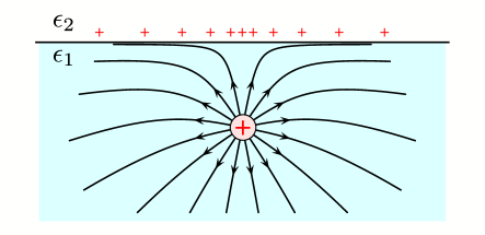
Figure 1: Field lines and induced surface charges for a point charge near an air-water or oil-water interface ($\epsilon_{1}\gg\epsilon_{2}$).

A more sophisticated approach is an implicit method which solves the Poisson equation with an inhomogeneous dielectric matched to the local composition. For example Groot Groot (2003a, b) introduced a particle-particle particle-mesh (P³M) method, with an underlying grid onto which the local dielectric permittivity is mapped. Implicit methods like Groot’s P³M typically require bespoke numerical codes, precluding the use of standard methods such as Ewald summation. But in addition, as Groot remarks, in an implicit dielectric method there must also be forces on the neutral solvent particles.

To see why this is the case, focus on Fig. 1 where a test charge $Q$ is embedded in a medium with a high dielectric permittivity (e. g. water) at a distance $h$ from an interface with a medium with a low dielectric permittivity (e. g. air, or oil). This textbook problem is readily solved to find the charge is repelled from the interface with a force $QQ^{\prime}/(16\pi\epsilon_{1}\epsilon_{0}h^{2})$, where $Q^{\prime}=Q(\epsilon_{1}-\epsilon_{2})/(\epsilon_{1}+\epsilon_{2})$ (the image charge) is located a distance $h$ on the opposite side of the interface. Of course, the image charge is just a convenient mathematical fiction introduced to solve the inhomogeneous electrostatic problem, and in reality the embedded charge is repelled by induced surface charges as shown in Fig. 1.

An implicit dielectric approach will certainly correctly calculate the force on the embedded charge due to the induced charges, but unless one takes into account the induced forces on solvent particles, the back reaction on the medium will be missed. Neglecting this leads to a situation in which there are unbalanced forces, with potentially disastrous consequences for the underlying physics. Other examples make the same point. For instance a well-known scientific parlour trick is to use a plastic comb charged by friction to pick up small bits of paper Feynman et al. (1963). This works because the bits of paper, although uncharged, are polarised by the inhomogeneous electric field of the static charges on the comb, and as such feel a force in this field. Now consider this from the point of view of an implicit dielectric simulation method where the dielectric body comprises solely neutral particles. If there are no induced forces on these particles, there is no force on the dielectric body in an inhomogeneous field, and a basic physical principle is violated. To counter this Groot argued the forces on neutral particles (such as solvent beads) can be neglected if spatial inhomogeneities are weak Groot (2003a). We agree, but by the same token the forces on the explicit charges (e. g. solute ions) due to induced image charges are similarly weak, and can also be neglected. If this is the case, there is no need to worry about spatial dielectric inhomogeneities in the first place.

Since computing the back-reaction forces in an implicit method is quite onerous, this leads us to explore a third explicit approach to modelling dielectric inhomogeneities, one in which we allow the dielectric properties to emerge naturally as a consequence of having explicitly polarisable solvent molecules in the model Wertheim (1979); Stell et al. (1981); Gray et al. (2011). In the models we shall explore below, the polarisability arises from partial charges on the (net electrically neutral) solvent molecules. In this approach, the static background dielectric permittivity is set to a constant (e. g. representative of a hydrocarbon oil phase) and dielectric inhomogeneities emerge spontaneously corresponding to the distribution of the polar solvent molecules. Induced charges are explicitly represented, by the disposition of the partial charges. The partial charges interact with other charges, such as the test charge in Fig. 1, through the normal Coulomb law. Force balance is satisfied at all times, and basic physical principles are fully respected.

The penalty introduced here is the need to solve the electrostatics problem including all the partial charges of the solvent molecules. These are of course usually much more numerous that any explicit charges thus there is a considerable additional computational cost. However, this cost replaces the laborious and bespoke calculation of the reaction forces on neutral solvent particles that we have just argued is required in an implicit method. On the other hand an immediate and clear advantage is that a well-stocked cabinet of molecular dynamics (MD) methods is available to deal with the electrostatics problem Allen and Tildesley (1987); Frenkel and Smit (2002). Mesh discretisation artefacts such as might be encountered using grid-based implicit methods are also obviously absent, but there is no free lunch: other artefacts may arise due to the finite size of the polar molecules, unwanted dielectric saturation, or an unphysical frequency response. Therefore a systematic approach is required.

Our aim here is to explore the properties of a broad class of polarisable soft solvent models in the paradigm just described, and in the context of dissipative particle dynamics (DPD) as a widely-used prototypical coarse-grained MD method Español and Warren (2017). In the rest of this paper we first describe the models and analysis methods, before reporting on the basic properties in terms of dielectric behaviour. We propose a couple of specific models which could be used for oil-water mixtures, and demonstrate the behaviour in test cases of increasing complexity.

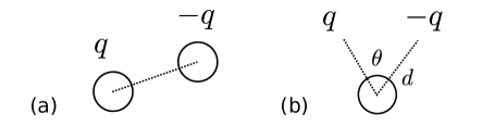
Figure 2: Polarisable soft solvent models: (a) molecular dimer comprising a bound pair of solvent beads carrying equal and opposite partial charges, (b) trimer comprising a single solvent bead dressed with a pair of tethered partial charges.

II Models

II.1 Design principles

In this work polarisable soft solvent models are built by adding partial charges to small solvent ‘molecules’. In constructing these models we shall attempt to minimally perturb the ‘standard’ DPD solvent model, which has seen considerable service underpinning various recent systematic parameterisation efforts Fraaije et al. (2016); R. L. Anderson, et al. (2017). This basic underlying model has solvent beads interacting with the standard short-range, pairwise, soft repulsions described by the pairwise interaction potential $\beta\phi(r)=A(1-r/r_{c})^{2}/2$ for $r\leq r_{c}$, and $\phi(r)=0$ for $r>r_{c}$, where $r$ is the bead-bead centre separation, $A$ is the repulsion amplitude, $r_{c}$ is a cut-off distance, and $\beta=1/k_{\text{B}}T$ is the inverse of the unit of thermal energy $k_{\text{B}}T$. In what follows we shall use $r_{c}$ and $k_{\text{B}}T$ for the simulation units of length and energy, and make the usual choice $\rho r_{c}^{3}=3$ for the bead density and $A=25$ for the repulsion amplitude Groot and Warren (1997).

Building on this, we consider two classes of polarisable solvent model (Fig. 2). In the dimer class (Fig. 2a), pairs of DPD solvent beads are joined by springs and assigned equal and opposite partial charges $\pm q$. Given the standard choice of bead density, the molecular density in this class is $\rho_{m}r_{c}^{3}={3}/{2}$. In the dressed solvent class (Fig. 2b), we shall keep the original solvent beads but to each solvent bead tether a pair of equal and opposite partial charges $\pm q$ by springs. In this class of trimer models the central beads interact only via the DPD soft repulsions, and partial charges only via electrostatics, thus severing the springs decouples the two systems. The molecular density in this case is $\rho_{m}r_{c}^{3}=3$.

The dimer class has a computational advantage since the density of partial charges is half that of the dressed solvent class, and is favourable if one is only interested in permittivity. However, a potential disadvantage is that the springs may intrude upon the solvent rheology. Additionally, Gaussian springs can stretch indefinitely under some flow conditions and FENE springs might be a better choice. Thus, apart from computational efficiency, one might disfavour this choice.

The dressed solvent class includes models initially investigated by Peter and Pivkin Peter and Pivkin (2014) and Peter, Lykov and Pivkin Peter et al. (2015), and refined recently by Vaiwala, Jadhav and Thaokar Vaiwala et al. (2018). These models can be regarded as an evolution of the Drude oscillator water model developed for the MARTINI force field Yesylevskyy et al. (2010); P. C. T. Souza, et al. (2021). The solvent dynamics in the dressed solvent class may also differ from that of the standard DPD solvent, but only indirectly via coupling to the electrostatics.

For both classes, the springs correspond to a bonding interaction potential given by $\beta\phi(d)=\frac{1}{2}k_{d}(d-d_{0})^{2}$ where $d$ is the separation between the force centres, $k_{d}$ is a spring constant, and $d_{0}$ the nominal bond length (which may be set to zero). In addition for the dressed solvent class of models we can allow for an angular spring $\beta\phi(\theta)=\frac{1}{2}k_{\theta}(\theta-\theta_{0})^{2}$ where $\theta$ is the angle subtended at the central bead by the partial charges, $k_{\theta}$ the angular spring constant, and $\theta_{0}$ the nominal opening angle.

II.2 Length scale mapping

The partial charges $\pm q$ are expressed in terms of the fundamental unit of charge, but before proceeding to this step it is first necessary to map $r_{c}$ into physical units. To do this, we follow the seminal lead of Groot and Rabone Groot and Rabone (2001) in introducing a solvent bead mapping number ${\cal N}_{m}$ (usually a small integer, but not necessarily so), which is the mean number of real solvent molecules represented by one DPD solvent bead. It follows that one mole of DPD ‘volume elements’ occupies a volume

$$N_{A}r_{c}^{3}=\rho r_{c}^{3}{\cal N}_{m}V_{m}\,,$$ (1)

where $V_{m}$ is the solvent molar volume and $N_{A}$ is Avogadro’s number; from this $r_{c}$ can be calculated. For example, with the common choice ${\cal N}_{m}=3$ to represent water ($V_{m}\approx 0.018\,\mathrm{L}\,\mathrm{mol}^{-1}$), we find $N_{A}r_{c}^{3}\approx 0.162\,\mathrm{L}\,\mathrm{mol}^{-1}$ assuming the solvent bead density $\rho r_{c}^{3}=3$ as above, which corresponds to $r_{c}\approx 0.646\,\text{nm}$. The identification of $r_{c}$ underpins the conversion of all lengths and molecular densities. We should emphasise that we do not expect the solvent molecular density and molecular polarisability in the coarse-grained model to be the same as those of the real system. Rather, the intent is that the solvent model should appear as a featureless dielectric continuum on length scales greater than $r_{c}$. Any residual effects of solvent granularity should be viewed as discretisation artefacts.

Throughout the rest of the paper we use DPD units, which amount to setting $k_{B}T=1$, $m=1$ and $r_{c}=1$ (that is, in using the thermal energy, DPD bead mass and radius as fundamental units). To help the reader in better grasping the corresponding physical scales, Table 1 gives the conversion for some key physical quantities, and the values of the reference quantities in SI units for our typical DPD mapping choice.

Physical quantity	DPD unit	Example value	unit
length	$r_{c}$	$0.646$	nm
electric field	$k_{\text{B}}T/(er_{c})$	$3.98\times 10^{7}$	$\mathrm{V}\,\mathrm{m}^{-1}$
electric dipole	$er_{c}$	$1.03\times 10^{-28}$	$\mathrm{C}\,\mathrm{m}$
		$=31.0$	D (Debye)
pressure	$k_{\text{B}}T/r_{c}^{3}$	15.3	MPa
surface tension	$k_{\text{B}}T/r_{c}^{2}$	$9.9$	$\mathrm{mN}\,\mathrm{m}^{-1}$
kinetic time scale	$r_{c}\sqrt{{m}/{k_{\text{B}}T}}$	$3.01$	ps

Table 1: DPD units and physical units for relevant physical quantities. The values in the third column correspond to the choice ${\cal N}_{m}=3$, $\rho r_{c}^{3}=3$ and room temperature ($T=298\,\mathrm{K}$).

II.3 Electrostatics

Now we turn to the specification of the electrostatics. In terms of the dielectric properties, we draw a careful distinction between the following quantities sub :

$$\begin{split}&\epsilon_{0}=\text{absolute permittivity of free space (vacuum)},\\ &\epsilon_{b}=\text{static background relative permittivity},\\ &\epsilon_{r}=\text{polarisable solvent relative permittivity}.\end{split}$$ (2)

The latter two are defined relative to free space (vacuum). We further define, relative to background,

$$\epsilon={\epsilon_{r}}/{\epsilon_{b}}\,.$$ (3)

The full permittivity of our polar solvent model for example is thus $\epsilon\epsilon_{b}\epsilon_{0}$.

The central problem addressed in the present work is to design a model which achieves a desired value of $\epsilon$. Thus for example, for water in coexistence with water vapour at room temperature, we should choose $\epsilon_{b}=1$, and aim for $\epsilon\approx 78$. We describe such pure water models in more detail in Sec. V. For another example, in a water-in-oil system we can choose for example $\epsilon_{b}=2$ for the oil oil , and then aim for $\epsilon\approx 39$ so that $\epsilon_{r}=\epsilon\epsilon_{b}\approx 78$ for the water. We note that in principle one could always use vacuum as a background and make the oil polarisable too, but this would increase the number of charges required in the simulation, since both fluids (oil and water) would comprise polar(isable) molecules, and consequently increase the computational time.

The long-range Coulomb law between unit charges in the static background (e. g. oil) fixes the Bjerrum length,

$$l_{\text{B}}=\frac{e^{2}}{4\pi\epsilon_{b}\epsilon_{0}k_{\text{B}}T}\,.$$ (4)

In practical terms, it is the dimensionless ratio $l_{\text{B}}/r_{c}$ that should be specified, or the dimensionless coupling parameter $\Gamma=4\pi l_{\text{B}}/r_{c}$. For instance if the static background is intended to be a hydrocarbon oil we might designate $\epsilon_{b}=2$ for which $l_{\text{B}}\approx 27\,\text{nm}$, and then $l_{\text{B}}/r_{c}\approx 42$ ($\Gamma\approx 530$), assuming the ${\cal N}_{m}=3$ mapping. For another example, for vacuum as background one would have $l_{\text{B}}\approx 55\,\text{nm}$ and $l_{\text{B}}/r_{c}\approx 85$ ($\Gamma\approx 1070$).

The final part of the electrostatics specification concerns charge smearing, which is required to prevent a ‘collapse’ since there are no hard cores Fisher and Ruelle (1966). Here we consider both Gaussian charge smearing Warren et al. (2013); Warren and Vlasov (2014), and Slater charge smearing González-Melchor et al. (2006); Ibergay et al. (2009); Vaiwala et al. (2017). For Gaussian charges the interaction potential (between partial charges) is

$$\beta\phi(r)=\frac{l_{\text{B}}q^{2}}{r}\operatorname{erf}\Bigl{(}\frac{r}{2\sigma}\Bigr{)}\,,$$ (5)

where $\sigma$ is the smearing length. For Slater partial charges (which are used in the models described in Sec. V) we use the approximate form

$$\beta\phi(r)=\frac{l_{\text{B}}q^{2}}{r}[1-(1+\beta^{\star}r^{\star})e^{-2\beta^{\star}r^{\star}}]\,,$$ (6)

where $\beta^{\star}=r_{c}/\lambda$, $r^{\star}=r/r_{c}$, and $\lambda$ is the Slater smearing length. In both of these the correct long-range Coulomb law is recovered for large separations.

To summarise: the polarisable solvent models we study are specified by the molecular parameters $k_{d}$, $d_{0}$, and additionally for trimers $k_{\theta}$, $\theta_{0}$ ; the magnitude of the partial charges $q$ ; the charge smearing scheme and length $\sigma$ or $\lambda$ ; the choice of static background $\epsilon_{b}$ which sets the Bjerrum length $l_{\text{B}}$ ; the repulsion amplitude between solvent beads $A$ ; the bead or molecular density $\rho_{m}$ ; and the ${\cal N}_{m}$ mapping choice which fixes $r_{c}$. The key target is the ratio $\epsilon=\epsilon_{r}/\epsilon_{b}$.

II.4 Specific models

Before listing the specific models used in the present work, let us make some general remarks. As mentioned, the central aim of a mesoscale polarisable solvent model is to provide a featureless dielectric continuum, in so far as the solvent beads are uniformly distributed. To achieve this we should endeavour to keep structural features and artefacts to length scales less than $r_{c}$. Following this line of argument, in order to get a large value of $\epsilon$ we should make the individual molecular dipoles as large as possible, but with a bond length not larger than $r_{c}$. This thinking drives the essential choices below. Nevertheless, it shall become apparent that there are dipole-dipole correlations in these models, which obliges care in applications.

In the dimer (DIM) class, we fix $\rho_{m}r_{c}^{3}=3/2$, $A=25$, $k_{d}=5$, $d_{0}=0$, and use Gaussian charge smearing with $\sigma=0.5$. Then $l_{B}$ and $q$ are varied to match the target system. In particular, for water in oil we suggest $(l_{B}/r_{c},q)=(42,0.463)$, and call the parameterisation WinO-DIM.

In the dressed solvent (DS) class, we fix $\rho_{m}r_{c}^{3}=3$, $A=25$, $k_{d}=10$, $d_{0}=0$, and use Gaussian smearing with $\sigma=0.5$. Here, for water in oil we suggest $(l_{B}/r_{c},q)=(42,0.36)$, and call the parameterisation WinO-DS. Within the same class, five other models obtained by varying the partial charge are considered (namely: $l_{B}/r_{c}=42$ and $q=0.08,0.1,0.2,0.3,0.4$). We call these parameterisations DS-q0.08, DS-q0.1, and so on. The dielectric properties are reported in Sec. IV.1, and for practical reasons some are used in the tests of Sec. IV.2.

In the codes the long range electrostatics part is dealt with by Ewald summation, as discussed in Appendix B, or in the case of dl_meso optionally also by smooth particle mesh Ewald (SPME) Essmann et al. (1995). In physical terms, neither $\sigma$ nor $\lambda$ should have any significance, and the actual choice is dictated by pragmatic considerations Warren et al. (2013); Warren and Vlasov (2014). For completeness, the parameterisations WinO-DIM and WinO-DS are reported in Table 2.

A subset of the dressed solvent class includes the Peter-Pivkin water-in-vacuum models Peter and Pivkin (2014); Peter et al. (2015) with strong harmonic bonds and the additional angle potential. Here we would like to highlight that they do not lead to the desired permittivity for water without modification. We discuss this class of model, including parameterisation challenges, more fully in Sec. V.

model class $\rightarrow$	dimer solvent	dressed solvent
parametrisation	WinO-DIM	WinO-DS
$r_{c}$	$0.646\,\text{nm}$	$0.646\,\text{nm}$
$A$	25	25
$k_{d}/r_{c}^{-2}$	5	10
$q$	0.463	0.36
$\sigma/r_{c}$	0.5	0.5
$l_{\text{B}}$	$27\,\text{nm}$	$27\,\text{nm}$
$l_{\text{B}}/r_{c}$	42	42
$\rho_{m}r_{c}^{3}$	3/2	3
$\langle{\Delta{\bf r}^{2}}\rangle/r_{c}^{2}$	0.669(1)	0.5660(5)
$g_{\text{C}}$	1.02(4)	1.05(5)
$\epsilon_{r}/\epsilon_{b}=\epsilon$	40(2)	42(2)
$g_{\text{K}}$	0.69(3)	0.70(2)
$\epsilon_{b}$ (oil)	2	2
$\epsilon_{r}$ (water)	80(4)	84(4)

Table 2: Parameters of the dimer solvent and dressed solvent models, with the values of $q$ and $l_{\text{B}}$ appropriate for water in oil. As explained in the text, the standard DPD soft repulsion acts between all beads in the dimer class, whereas only between neutral beads in the dressed solvent class. The dielectric properties (see Sec. II.3, III.3 and III.4) are computed here from Monte-Carlo simulations (see also Table 3). A figure in brackets here and elsewhere is an estimate of the error in the final digit.

III Methods

III.1 Simulations

We study the properties of the models introduced above with a combination of dissipative particle dynamics (DPD) using dl_meso Seaton et al. (2013) ECA , and Monte-Carlo (MC) simulations using a bespoke code. Whereas dl_meso can be applied to a wide variety of interesting problems, the MC code is limited to generating homogeneous solvent configurations to compute structural and thermodynamic solvent properties, including of course the relative permittivity $\epsilon=\epsilon_{r}/\epsilon_{b}$.

For the DPD simulations, unless otherwise stated, the typical simulated volume is a cubic box of side $L=10$. The time step is always $\delta t=0.01$, and simulations are typically run for $5\times 10^{5}$ time steps, after $10^{4}$ equilibration steps. Sampling is done every 100 steps. The DPD drag coefficient is $\gamma=4$.

Whilst dl_meso is well documented, we here provide some brief details of the MC code, which was based on earlier work Warren et al. (2013). For present purposes this was configured to run in an $NVT$ ensemble, with single-particle trial displacements. A standard Metropolis scheme is implemented Frenkel and Smit (2002), with trial displacements $\delta r=0.25$–0.4 chosen to obtain an acceptance rate of 30–50%. We typically consider cubic boxes of side $L=8$, and typically equilibrate for $3\times 10^{5}$ trial MC moves before sampling the configuration every $1.5\times 10^{5}$ trial moves. One can show that this is sufficient to allow all the particles to move a distance of order 1–$2\,r_{c}$ between sampled configurations. A large number (500–1000) of samples are required to estimate the mean square box dipole moment with sufficient accuracy. We achieve this in part by task-farming across a 100+ node cluster (at the expense of having to equilibrate on each node).

Benchmarking dl_meso against the MC code allows us to test for issues due to incomplete equilibration, as well as possible artefacts coming from the DPD thermostat (which, recall, is a pairwise spring-dashpot type); no significant effects were found. Also, the independently developed MC code uses interparticle potentials, whereas dl_meso uses interparticle forces, which provides a stringent test for coding errors in the implementation of the electrostatics, and in fact in the course of the work we uncovered a problem with the implementation of Slater smearing in dl_meso which can be traced to an incorrect expression for the forces in the literature Ibergay et al. (2009); it was obviously fixed for the present study. For completeness, in Appendix B we document the nature of the problem and provide some precision benchmark MC results for the reference Slater charge plasma (see below).

To summarise, dl_meso and the bespoke MC code are found to be in excellent mutual agreement. This gives us a high degree of confidence in the results.

III.2 Liquid state theory

For supporting calculations we shall occasionally use a liquid state theory to calculate the structural properties of multicomponent charged fluids (plasmas). This was developed for our previous work Warren et al. (2013); Warren and Vlasov (2014), and uses the hypernetted chain (HNC) approximation to close the Ornstein-Zernike equations Hansen and McDonald (2006). The HNC is known to yield particularly accurate results for soft potentials Fraaije et al. (2016), and takes proper account of the electrostatics such as the Stillinger-Lovett sum rules Hansen and McDonald (2006). Some benchmark results related to the present problem are included in Table 8 in Appendix B.

III.3 Dielectric permittivity

To calculate the relative dielectric permittivity, we use either dl_meso or MC to generate configurations of $N_{m}$ solvent molecules in a cubic simulation box of volume $L^{3}=V$. Then, in linear response theory, the dielectric constant can be computed from fluctuations in the box dipole moment as described in Frenkel and Smit Frenkel and Smit (2002), Allen and Tildesley Allen and Tildesley (1987), and Kusalik et al. Kusalik et al. (1994). Note that there is scope for considerable confusion over units here, with some authors preferring Gaussian (cgs) units, and others using bespoke reduced units. In the present work we shall formulate the problems initially using SI units, but switch to writing expressions in terms of the Bjerrum length $l_{\text{B}}$ where practically possible.

For the most part we adopt the so-called ‘tin-foil’ or conducting boundary conditions since this gives the most accurate results for a given computational cost Allen and Tildesley (1987). To summarise the calculation in the present context, let the dipole of the $i$-th solvent molecule be ${\bf p}_{i}$ and the total dipole moment in the simulation box be ${\bf P}_{\text{box}}=\sum_{i=1}^{N_{m}}{\bf p}_{i}$ box . Then Allen and Tildesley (1987); Frenkel and Smit (2002)

$$\epsilon=1+\frac{\langle{{\bf P}_{\text{box}}^{2}}\rangle}{3\epsilon_{b}\epsilon_{0}Vk_{\text{B}}T}\,,$$ (7)

where, to recall, $\epsilon={\epsilon_{r}}/{\epsilon_{b}}$ is the permittivity of the polarisable solvent relative to the static background, and $\langle{\dots}\rangle$ denotes an ensemble average. Note that the static background relative permittivity features also in the denominator on the right-hand side of this equation.

In terms of the Bjerrum length defined in Eq. (4), the above expression can be written as

$$\epsilon=1+3yg_{\text{C}}\,,$$ (8)

where $y={4\pi l_{\text{B}}\rho_{m}\langle{{\bf p}^{2}}\rangle}/{9e^{2}}$ and $g_{\text{C}}={\langle{{\bf P}_{\text{box}}^{2}}\rangle}/{N_{m}\langle{{\bf p}^{2}}\rangle}$, following an established notation Allen and Tildesley (1987); Hansen and McDonald (2006). Here $\rho_{m}=N_{m}/V$ is the number density of solvent molecules, $\langle{{\bf p}^{2}}\rangle$ is the mean square molecular dipole moment, and the subscript ‘C’ on $g_{\text{C}}$ signals the choice of (conducting) boundary conditions.

The solvent molecules in our models have equal and opposite partial charges, so in practical terms ${\bf p}_{i}=qe\Delta{\bf r}_{i}$ where $\Delta{\bf r}_{i}$ is the vector from $-q$ to $q$. We additionally define $\Delta{\bf R}=\sum_{i=1}^{N}\Delta{\bf r}_{i}$. For charge smeared models, the charge clouds are centro-symmetric and $\Delta{\bf r}_{i}$ is measured between the charge cloud centres. From these,

$$y=\frac{4\pi l_{\text{B}}q^{2}\rho_{m}\langle{\Delta{\bf r}^{2}}\rangle}{9}\,,\quad g_{\text{C}}=\frac{\langle{\Delta{\bf R}^{2}}\rangle}{N_{m}\langle{\Delta{\bf r}^{2}}\rangle}\,.$$ (9)

The values of $\langle{\Delta{\bf r}^{2}}\rangle$ and $\langle{\Delta{\bf R}^{2}}\rangle$ required in these expressions (in units of $r_{c}^{2}$) can be obtained from a time series of simulation snapshots. Care is taken to ensure the simulation snapshots are uncorrelated, by measuring the time autocorrelation function for $\Delta{\bf R}$. Errors are estimated by block averaging, and further controlled by replicate simulation runs.

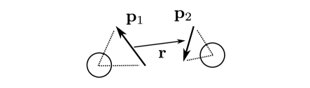
Figure 3: Geometry for molecular dipole distribution functions: for each pair of solvent dipoles (here illustrated for the trimer model) we define the dipole moments ${\bf p}_{1}$ and ${\bf p}_{2}$, and the distance between the dipole centers ${\bf r}$.

Parametrisation		DS-q0.08	DS-q0.1	DS-q0.2	DS-q0.3	WinO-DS (or DS-q0.36)		DS-q0.4
Method	Quantity	$q=0.08$	$q=0.1$	$q=0.2$	$q=0.3$	$q=0.36$	[$\epsilon^{\prime}=42$]	$q=0.4$
DPD	$\langle{\Delta{\bf r}^{2}}\rangle/r_{c}^{2}$	0.5926(5)	0.5898(3)	0.5785(3)	0.5709(3)	0.5669(3)		0.5648(3)
	$g_{\text{C}}$	1.00(2)	1.02(3)	1.08(3)	1.08(3)	1.07(3)		1.00(4)
	$\epsilon_{r}/\epsilon_{b}=\epsilon$	2.99(5)	4.18(9)	14.2(4)	30.3(8)	42(1)		49(2)
	$g_{\text{K}}$	0.78(1)	0.76(2)	0.75(2)	0.73(2)	0.72(2)		0.67(3)
Monte-Carlo	$\langle{\Delta{\bf r}^{2}}\rangle/r_{c}^{2}$	0.593(1)	0.590(1)	0.579(1)	0.571(1)	0.5660(5)	0.5660(4)	0.564(1)
	$g_{\text{C}}$	1.03(6)	1.05(6)	1.01(6)	1.02(3)	1.04(4)		1.09(3)
	$\epsilon_{r}/\epsilon_{b}=\epsilon$	3.1(1)	4.3(2)	13.4(7)	29(2)	41(2)	43(2)	53(2)
	$g_{\text{K}}$	0.80(4)	0.78(4)	0.70(4)	0.69(2)	0.70(2)	0.72(2)	0.73(2)
pressure	$r_{c}^{3}{\mathfrak{p}}/k_{\text{B}}T$	23.64(2)	23.62(2)	23.50(2)	23.37(2)	23.26(1)		23.21(2)
Wertheim	$\langle{\Delta{\bf r}^{2}}\rangle/r_{c}^{2}$	0.5948	0.5934	0.5874	0.5830	0.5809		0.5796
Onsager	$\epsilon_{r}/\epsilon_{b}$	3.65	5.29	19.1	42.1	60.1		73.9

Table 3: Tabulated results for all dressed solvent models as a function of partial charge. Results are shown for DPD using dl_meso and for comparison from Monte-Carlo simulations, for which we also report the pressure ${\mathfrak{p}}$. Generally, the first two rows are computed directly from simulation, being the mean square molecular dipole length $\langle{\Delta{\bf r}^{2}}\rangle$, and the factor $g_{\text{C}}=\langle{\Delta{\bf R}^{2}}\rangle/N_{m}\langle{\Delta{\bf r}^{2}}\rangle$ computed under conducting boundary conditions. These are used to calculate the relative permittivity $\epsilon_{r}/\epsilon_{b}$ (third row) from Eqs. (8) and (9), and the Kirkwood factor $g_{\text{K}}$ (fourth row) from Eq. (14). The penultimate row labelled ‘Wertheim’ is from the theory in Sec. III.5 with the plasma reference correction; without this the entries would all be $\langle{\Delta{\bf r}^{2}}\rangle/r_{c}^{2}=3/5=0.6$. The final row utilises Onsager theory to estimate the relative permittivity from Eq. (17), which assumes $g_{\text{K}}=1$. For the WinO-DS model ($q=0.36$), an extra column is inserted for properties computed in Monte-Carlo with a reaction field, where the embedding medium relative permittivity is set to $\epsilon^{\prime}=42$ to match that of the fluid (or, close enough for present purposes).

III.4 Correlation functions

To quantify the structural properties we examine the solvent bead pair distribution function, $g_{00}(r)$, and the molecular dipole-dipole correlation functions following Stell et al. Stell et al. (1981). For the latter we introduce a number of radially-resolved moment correlation functions (see Fig. 3 for the geometry),

$$\begin{array}[]{l}g_{000}(r)=\langle{1}\rangle_{r}\,,\quad g_{110}(r)=\langle{{\bf p}_{1}\cdot{\bf p}_{2}}\rangle_{r}\,,\\[3.0pt] g_{112}(r)=\langle{\frac{3}{2}({\bf p}_{1}\cdot\hat{{\bf r}})({\bf p}_{2}\cdot\hat{{\bf r}})-\frac{1}{2}{\bf p}_{1}\cdot{\bf p}_{2}}\rangle_{r}\,,\end{array}$$ (10)

where $r=|{\bf r}|$, $\hat{{\bf r}}={\bf r}/r$, and $\langle{\dots}\rangle_{r}$ indicates a radially-resolved average. For normalisation we ensure $g_{000}(r)\to 1$ as $r\to\infty$ so that it behaves like a standard pair distribution function, and for the higher moments we ensure that $\int\mathrm{d}^{3}{\bf r}\,g_{110}(r)\equiv(1/N_{m})\sum_{i\neq j}\langle{{\bf p}_{i}\cdot{\bf p}_{j}}\rangle$ , and mutatis mutandis for $g_{112}$.

These correlation functions (involving dipole moments) should be measured under matched or ‘Kirkwood’ boundary conditions in which the dielectric permittivity of the embedding medium is the same as that of the system itself, otherwise there are spurious artefacts on the length scale of the simulation box g (11). To simulate under these conditions one needs to include, in addition to the inter-particle potential, a ‘reaction field’ term Allen and Tildesley (1987); Frenkel and Smit (2002), which in terms of the Bjerrum length is

$$\beta\phi_{\text{pol}}=\frac{2\pi l_{\text{B}}{\bf P}_{\text{box}}^{2}}{(2\epsilon^{\prime}+1)Ve^{2}}\,.$$ (11)

The permittivity $\epsilon^{\prime}$ in here is that of the embedding medium (relative to background), which should be matched to that of the fluid (i. e. $\epsilon^{\prime}=\epsilon$). This means that the relative permittivity $\epsilon$ of the fluid should be pre-computed, for instance using conducting boundary conditions as described in the preceeding section.

Under these matched ($\epsilon^{\prime}=\epsilon$) boundary conditions, the expression in Eq. (8) for the dielectric permittivity is replaced by the Onsager-Kirkwood expression Allen and Tildesley (1987); Frenkel and Smit (2002); Böttcher (1973),

$$\frac{(\epsilon-1)(2\epsilon+1)}{9\epsilon}=yg_{\text{K}}\,.$$ (12)

Here the ‘Kirkwood factor’ $g_{\text{K}}={\langle{{\bf P}_{\text{box}}^{2}}\rangle}/{N_{m}\langle{{\bf p}^{2}}\rangle}=\langle{\Delta{\bf R}^{2}}\rangle/N_{m}\langle{\Delta{\bf r}^{2}}\rangle<g_{\text{C}}$ , since $\phi_{\text{pol}}$ acts to suppress fluctuations in the box dipole moment, making $\langle{{\bf P}_{\text{box}}^{2}}\rangle$ smaller than under conducting boundary conditions. On the other hand, to $O(1/N_{m})$, $\langle{{\bf p}^{2}}\rangle$ is unaffected by the choice of boundary conditions Gray et al. (2011).

Since $\langle{{\bf P}_{\text{box}}^{2}}\rangle=N_{m}\langle{{\bf p}^{2}}\rangle+\sum_{i\neq j}\langle{{\bf p}_{i}\cdot{\bf p}_{j}}\rangle$ , the Kirkwood factor can also be computed from $g_{110}(r)$ as

$$g_{\text{K}}=1+\frac{1}{\langle{{\bf p}^{2}}\rangle}\int_{0}^{\infty}\!\!\mathrm{d}r\;4\pi r^{2}\,g_{110}(r)\,.$$ (13)

Thus $g_{110}(r)$ quantifies the dipole-dipole correlations which contribute to $g_{\text{K}}\neq 1$. For completeness, the function $g_{112}(r)$ is included in the list of computed correlation functions, and the corresponding integral is, apart from a constant of proportionality, approximately the energy associated with the dipoles (exactly so, for true point dipoles).

Since $\langle{{\bf p}^{2}}\rangle$ and therefore $y$, as defined below Eq. (8), are unaffected by the choice of boundary conditions, eliminating $y$ between Eqs. (8) and (12) obtains

$$\frac{g_{\text{K}}}{g_{\text{C}}}=\frac{2\epsilon+1}{3\epsilon}\,.$$ (14)

This allows us to compute the Kirkwood factor $g_{\text{K}}$, given the value of $g_{\text{C}}$ computed under conducting boundary conditions and the permittivity $\epsilon$.

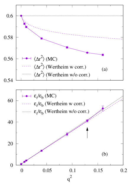
Figure 4: Dielectric properties of dressed solvent models in Table 3, as a function of $q^{2}$: (a) mean square dipole length $\langle{\Delta{\bf r}^{2}}\rangle$, and (b) relative permittivity $\epsilon=\epsilon_{r}/\epsilon_{b}$; the arrowed point is the WinO-DS model (Table 2), with $q=0.36$ and $\epsilon=42\pm 2$. Markers with error bars are Monte-Carlo simulations (error bars not shown in (a) as the error is smaller than markers). Lines are liquid state theory predictions with (dashed lines) and without (dotted lines) the plasma reference state correction.

III.5 Wertheim and Onsager theories

A relatively simple liquid state theory can be used to predict the value of $\langle{\Delta{\bf r}^{2}}\rangle$ in the above section, and from there the permittivity itself. The approach is rigorously based in Wertheim perturbation theory and more details will be presented elsewhere Mas . The first-order theory results in an approximate expression for the probability distribution ${\mathcal{P}}(\Delta r)$ for the distance $\Delta r$ between partial charges, with

$${\mathcal{P}}(r)=C\exp[-\beta\phi^{\text{int}}_{+-}(r)]\>g^{\text{ref}}_{+-}(r)\,.$$ (15)

Here $C$ is such that $4\pi\int_{0}^{\infty}\mathrm{d}r\,r^{2}\,{\mathcal{P}}(r)=1$. In Eq. (15), $\phi^{\text{int}}_{+-}(r)$ is the intramolecular pair potential between the partial charges arising from the bonds and $g^{\text{ref}}_{+-}(r)$ is the pair distribution function between the partial charges in a reference system in which all the bonds have been cut. Given all this,

$$\langle{\Delta{\bf r}^{2}}\rangle\approx 4\pi\int_{0}^{\infty}\!\!\mathrm{d}r\;r^{4}\,{\mathcal{P}}(r)\,.$$ (16)

Details of the intramolecular potentials for the models studied in the present work are given in Appendix A.

In the reference system (i. e. where the intramolecular bonds have been cut) $g^{\text{ref}}_{+-}$ is the pair distribution function between unlike charges in a neutral two-component plasma, at a total number density set by the original molecular solvent density ($\rho_{m}$ for the dimer case, $2\rho_{m}$ for the trimer case). In the following sections, we refer to such a reference system as a reference plasma. To calculate $g^{\text{ref}}_{+-}$ we can therefore deploy the HNC liquid state theory described in Sec. III.2. However, since the plasma is generally weakly coupled, one can already get quite accurate predictions by setting $g^{\text{ref}}_{+-}=1$. This gives estimates for $\langle{\Delta{\bf r}^{2}}\rangle$ in some cases in a closed analytic form. In principle higher order terms can be included in the perturbation expansion, but these are harder to calculate Mas .

This now allows us to compute $y$ from the first of Eqs. (9), and from this $\epsilon$ itself can be estimated using Onsager theory Böttcher (1973) in the form $(\epsilon-1)(2\epsilon+1)/\epsilon=9y$, which solves to

$$\epsilon\approx\frac{{1+9y+3\surd({1+2y+9y^{2}})}}{4}\,.$$ (17)

Onsager theory is equivalent to setting $g_{\text{K}}=1$ in (the exact) Eq. (12), and so involves the further approximation of the neglect of the dipole-dipole correlations. The more familiar (but even more approximate) Clausius-Mossotti relation, namely $(\epsilon-1)/(\epsilon+2)=y$, cannot be used if $y>1$ (which is usually the case here) since that lies outside its domain of validity Böttcher (1973).

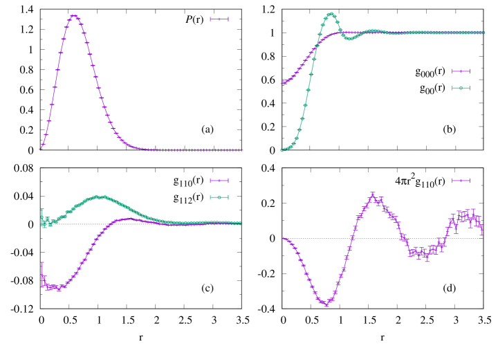
Figure 5: Correlation functions for the WinO-DS model (Table 2): (a) dipole length distribution, (b) central bead pair distribution function $g_{00}(r)$ and dipole-dipole centre distribution function $g_{000}(r)$, (c) and (d) higher order dipole-dipole correlation functions $g_{110}(r)$ and $g_{112}(r)$. The functions in (c) and (d) are normalised by dividing by $\langle{{\mathbf{p}}^{2}}\rangle$. These functions are computed using matched ‘Kirkwoood’ boundary conditions, with $\epsilon^{\prime}=42$ in the reaction field, as described in Sec. III.4 (see also Table 3).

IV Results

In this section we report on the dielectric properties of the proposed solvent models, then describe a series of problems that allow us to test them. Concrete examples are given for the class of dressed solvent (DS) model.

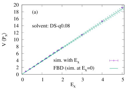
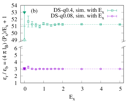
Figure 6: Application of an external electric field. (a) Mean polarisation under an applied field (points), compared to prediction from Eq. (19) in the text (lines) using $\epsilon_{r}/\epsilon_{b}=2.99(5)$ from the fluctuating box dipole method (Table 3). (b) Relative permittivity computed from this response as a function of the applied field. Results are from DPD simulations with dressed solvent models having $q=0.08$ and $q=0.4$. The horizontal lines are fits. For comparison, points at $E_{x}=0$ show the prediction from the fluctuating box dipole method in DPD (open upward triangles) and MC (filled downward triangles).

IV.1 Dielectric properties

As already described, we have explored the properties of both the dimer solvent and dressed solvent models. Our results for the dimer solvent are similar to those for the dressed solvents, and so we report only on the latter in detail. The relative permittivity $\epsilon=\epsilon_{r}/\epsilon_{b}$ and the $g_{\text{C}}$ factor are given in the second column in Table 2 for the water-in-oil dimer model ‘WinO-DIM’, in Table 3 and Fig. 4 for the dressed solvent models in general, and in the third column in Table 2 for the water-in-oil specific model ‘WinO-DS’. Apart from certain simulations of the WinO-DS model, all these results are obtained using the fluctuating box dipole method with conducting boundary conditions as described in Sec. III.3. To gain insight into the rôle of dipole-dipole correlations, the Kirkwood factor $g_{\text{K}}$ is included, calculated from $\epsilon$ and $g_{\text{C}}$ using Eq. (14).

For the majority, we compute these properties both using the dl_meso DPD code, and separately with our bespoke Monte-Carlo (MC) code. We find excellent agreement between these, which gives us a high degree of confidence in the results.

We also report the MC pressure for the dressed solvent models, observing that it diminishes very slightly with increasing $q$ because of the net cohesive effect of adding the partial charges, but is otherwise very close to the canonical DPD solvent ($\rho r_{c}^{3}=3$, $A=25$) for which we find the pressure in reduced units $r_{c}^{3}{\mathfrak{p}}/k_{\text{B}}T=23.65\pm 0.02$. This suggests that the addition of tethered partial charges in these models is only minimally perturbative to the underlying DPD solvent model.

For the dielectric properties, we can see from Table 3 and Fig. 4a that the mean square dipole length $\langle{\Delta{\bf r}^{2}}\rangle$ is relatively insensitive to the magnitude of the partial charges, although it decreases somewhat with increasing $q$, which is to be expected as opposite charges attract. For the dressed solvent models, in the absence of a plasma correction $\langle{\Delta{\bf r}^{2}}\rangle=3k_{\text{B}}T/(k_{d}/2)$ by equipartition, where $k_{d}/2$ is the effective spring constant, as argued in Appendix A. This results in $\langle{\Delta{\bf r}^{2}}\rangle=3/5$ since $k_{d}=10$, which is already close to the reported results. If the plasma reference correction is additionally included, as in Sec. III.5, then the agreement between the theory (Wertheim) and the model improves still further, as seen by comparing the corresponding rows in Table 3.

By far the biggest controlling factor for the relative dielectric permittivity is therefore the magnitude of $q$, and this is the reason we chose this as the main adjustable parameter in our models. The dependence of $\epsilon=\epsilon_{r}/\epsilon_{b}$ on $q$ is shown in Fig. 4b, which indicates that $\epsilon$ grows approximately linearly in $q^{2}$ for $\epsilon\gg 1$. As a design criterion, this observation allows us to relatively easily build models to reproduce targeted values of the dielectric permittivity. This will be illustrated in relation to the Peter-Pivkin water-in-vacuum models in Sec. V.

The Kirkwood factor is roughly constant across all the models, including the dimer model WinO-DIM, and takes the value $g_{\text{K}}\approx 0.7$–0.8. This indicates that dipole-dipole correlations are not negligible in these models. This is verified by the correlation functions calculated for WinO-DS model, shown in Fig. 5. Note in particular the damped oscillatory nature of $g_{110}(r)$ whose integral is directly related to $g_{\text{K}}$ by Eq. (13). As mentioned, these correlation functions are computed under matched boundary conditions, by including the appropriate reaction field and utilising the relative permittivity computed under conducting boundary conditions. This allows also a direct computation of $g_{\text{K}}$ and a separate estimate of the relative permittivity, which are found to be in excellent agreement with those calculated using conducting boundary conditions (see columns labelled WinO-DS in Table 3).

Given that the Kirkwood factor $g_{\text{K}}\approx 0.7$–0.8, Onsager theory (final row in Table 3) over-predicts the dielectric permittivity by approximately 20–30%. Nevertheless, the combination of Wertheim and Onsager allows a useful initial estimate of these properties, before resorting to simulation.

IV.2 Test problems

Here, various physical situations are analyzed to confirm that the solvent behaves as expected, i. e. as a medium having the dielectric permittivity as determined by the fluctuating box dipole method. DPD simulations with models belonging to the dressed solvent class are used for this purpose.

In the presence of an electric field, the polarisation density from classical electrostatics is ${\bf P}=(\epsilon_{r}-1)\epsilon_{0}{\bf E}$. For our polarisable molecular solvent with a background relative permittivity, this generalises to the induced polarisation of the solvent (i. e. the response of the partial charges),

$${\bf P}=(\epsilon-1)\epsilon_{b}\epsilon_{0}{\bf E}\,,$$ (18)

where, as usual and as a reminder, $\epsilon=\epsilon_{r}/\epsilon_{b}$.

All three methods below can be reverse-engineered to calculate the ratio $\epsilon_{r}/\epsilon_{b}$ and the results are summarised in Table 4, compared to the consensus results from fluctuating box dipole method using DPD and MC. In general the agreement is very good. As a practical comment, we note that measuring the induced polarisation with an applied electric field is the most accurate of these.

Parametrisation		DS-q0.08	DS-q0.4
Method	Refer to	$q=0.08$	$q=0.4$
Fluctuating box dipole	Table 3	3.0(1)00	51(2).00
Applied field	Sec. IV.2.1	3.021(3)	51.24(1)
Force reduction	Sec. IV.2.2	3.03(4)0	44(7).00
Charge screening	Sec. IV.2.3	3.00(7)0	—

Table 4: Values of $\epsilon_{r}/\epsilon_{b}$ from various tests described in the main text, compared to the consensus (DPD and MC) values using the fluctuating box dipole method (FBD) reported in Table 3, for dressed solvent models with the indicated values of the partial charge $q$.

IV.2.1 Application of an electric field

As a first test, an electric field $E_{x}$ along the $x$ direction is applied to a simulation box containing the polarisable solvent molecules at the standard density, and the resulting average polarisation is measured. In Fig. 6a this direct response (points) is compared with the linear response expected using the permittivity from the fluctuating box dipole method (solid line).

In reduced units, Eq. (18) becomes for this problem

$$\frac{q\Delta R_{x}r_{c}^{2}}{V}=\Bigl{(}\frac{\epsilon_{r}}{\epsilon_{b}}-1\Bigr{)}\,\frac{r_{c}}{4\pi l_{\text{B}}}\times\frac{er_{c}E_{x}}{k_{\text{B}}T}\,.$$ (19)

The quantity on the left-hand side is the polarisation density in the box in reduced units, and the second factor on the right-hand side is the electric field expressed as a force per unit charge, again in reduced units. Measuring the slope of the response therefore allows us to compute $\epsilon_{r}/\epsilon_{b}$, which is shown for dressed solvent models with $q=0.08$ and $q=0.4$ in Fig. 6b, with the final results reported in Table 4. In general, a good agreement is found, confirming that the dielectric responds linearly to the external field, for the field strengths considered, i. e. at least up to $5k_{\text{B}}T/(er_{c})$.

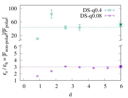
Figure 7: Force reduction (points) as function of the distance between the charges, $d/r_{c}$, and its best estimate for $d>2r_{c}$ (dashed lines). Results are from DPD simulations with test charges $Q=\pm 5$ in dressed solvent models with $q=0.08$ or $q=0.4$. Note that points for $q=0.4$ and $d>4r_{c}$ are not shown, as $F_{\text{polar}}$ is too small to be measured. For comparison, points at large $d$ show the prediction from the fluctuating box dipole method in DPD (open upward triangles) and MC (filled downward triangles).

IV.2.2 Force between two test charges

In this second test, two charges $\pm Q$ are fixed at a distance $d$ from each other and embedded in a solvent. Passing from an apolar to a polar medium, the force acting on each one is reduced by a factor $\epsilon_{b}/\epsilon_{r}=|F_{\text{polar}}|/|F_{\text{non-polar}}|$. Since we work with simulation boxes with periodic boundary conditions, what is actually reported here is the force reduction per charge, averaged over the three axis directions, and both ions, for a pair of interleaved, infinite cubic arrays of equal and opposite charges, separated by a distance $d$ along the diagonal.

In Fig. 7 we show results for the force reduction (points) as a function of $d/r_{c}$. The polar (non-polar) medium is represented here by the dressed solvent model with $q\neq 0$ ($q=0$), and we choose $Q=\pm 5$. For large enough $d$, it can be seen that the force reduction agrees nicely with $\epsilon_{r}$ from the fluctuating box dipole method (the ratio $\epsilon_{r}/\epsilon_{b}$ extracted from fitting the large separation reduction to a constant is given in Table 4). However, at low $d$, $F_{\text{polar}}$ is instead stronger than predicted by classical electrostatic theory: this lack of screening is an artefact of the model, related to the finite size of the solvent molecules. We note in passing that, to be able to detect this force-reduction effect, low $\epsilon_{r}/\epsilon_{b}$ and large $Q/q$ are needed: in the bottom part of Fig. 7, $\epsilon_{r}/\epsilon_{b}\simeq 3$, and $Q/q\simeq 63$.

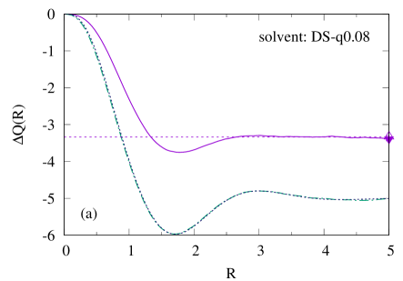
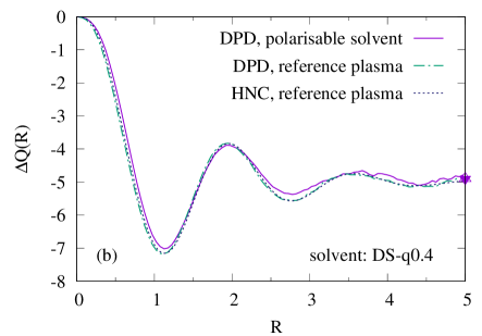
Figure 8: Solvent charge $\Delta Q(R)$ defined by Eq. (21) in the text (solid lines), in a sphere of radius $R$ centered on a test charge $Q=5$, in dressed solvent models with (a) $q=0.08$ and (b) $q=0.4$. Also shown for comparison is $\Delta Q(R)$ for a test charge in a reference plasma, computed by DPD (chain lines) and compared to HNC (dotted lines). As in previous figures, points at large $R$ show the prediction from the fluctuating box dipole method in DPD (open upward triangles) and MC (filled downward triangles).

IV.2.3 Screening around a test charge

The electric field around a test charge $Q$ embedded in our polarisable solvent is partially screened by the dielectric response to ${\bf E}={Q{\bf r}}/{4\pi\epsilon_{r}\epsilon_{0}r^{3}}$. Using Eq. (18) again, this implies an induced polarisation ${\bf P}=(\epsilon-1)Q{\bf r}/4\pi\epsilon r^{3}$. Since $\nabla\cdot({\bf r}/r^{3})=4\pi\,\delta^{3}({\bf r})$, this corresponds to an induced polarisation charge located exactly on top of the test charge, of magnitude and sign

$$\Delta Q=-\Bigl{(}1-\frac{\epsilon_{b}}{\epsilon_{r}}\Bigr{)}\,Q\,.$$ (20)

As another test therefore, we compute the solvent charge (i. e. from the partial charges) contained in a sphere of radius $R$ centered on a positive ion $Q$. Microscopically, this can be written in terms of the pair distribution functions between the test charge and the partial solvent charges, as

$$\Delta Q(R)=4\pi\rho_{m}q\int_{0}^{R}\!\!\mathrm{d}r\,r^{2}\,[g_{Q+}(r)-g_{Q-}(r)]\,.$$ (21)

We expect this to saturate to the value given in Eq. (20) as $R\to\infty$ (i. e. beyond the dipole-dipole correlation length).

In Fig. 8 we show the solvent charge $\Delta Q(R)$ computed as a function of the sphere radius $R$ around a test charge $Q=5$ , for dressed solvent models with small ($q=0.08$) and large ($q=0.4$) permittivities scr . In addition, we also show results for a test charge embedded in the reference plasma of Sec. III.5 (i. e. the solvent with the partial charges cut loose), and compare this to HNC calculations of the same (i. e. using a three-component system with a vanishingly small density of test charges). For all cases it can be seen that after a few damped oscillations $\Delta Q(R)$ becomes constant, attaining the expected value from Eq. (20) in the solvent (partial screening) and $-Q$ in the plasma (total screening). The damped oscillations, which persist in the reference plasma and are corroborated by HNC results, reflect the charge ordering taking place in a strong dielectric: see, for example, Keblinski et al. Keblinski et al. (2000). Note that in the negative arms of the oscillations the charge compensation is larger than the test charge itself, $|\Delta Q|>Q$, indicating overscreening locally.

We can use Eq. (21) in the limit of large $R$, with Eq. (20), to back out the ratio $\epsilon=\epsilon_{r}/\epsilon_{b}$. This only really works for the case where $\epsilon$ is not too large otherwise we cannot distinguish between partial screening and total screening (cf. Fig. 8b) which is also the limit of Eq. (20) as $\epsilon_{r}\to\infty$. Such a situation determines $\epsilon_{r}/\epsilon_{b}$ very imprecisely, and we therefore report only the result for $q=0.08$ in Table 4.

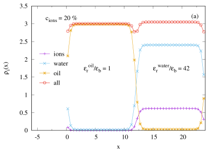
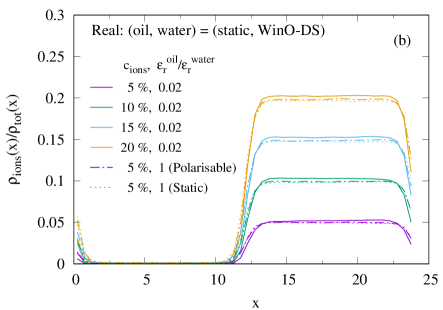
Figure 9: Desorption of ions from an oil/water interface. Results are from DPD simulations with ions of charge $\pm 1$ and the dressed solvent model with $q=0.36$ or $q=0$. See text for more details.

IV.3 Ion desorption from oil/water interface

We now turn to a less trivial example demonstrating that our model shows ion desorption from an oil/water interface of the kind alluded to in the introduction. We recall from that discussion that a point charge of any sign, embedded in a certain medium, is repelled from an interface with a medium of lower $\epsilon_{r}$. In the limit of infinite dielectric contrast, it effectively sees an identical image charge across the interface.

Accordingly, as a fourth test, we consider two immiscible solvents, oil and water, and add ions at various concentrations in the water phase. The DPD repulsion parameter is tuned to ensure immiscibility and to prevent the ions from leaving the water phase: $A=40$ between water and oil and between ions and oil (for water and oil, we intend between their neutral beads), whereas for intra-solvent interactions and between ions we keep $A=25$. To reproduce the real dielectric permittivity mismatch between water and oil, we use the dressed solvent model with $q=0.36$ (for water) and with $q=0$ (for oil).

We then observe the ionic density profiles and compare them with controls in which there is no dielectric mismatch, by arranging for the oil and water permittivities to be equal (with both set to the water value). For these controls, we either set $q=0$ for both oil and water, with a static background $l_{B}=1$ ; or set $q=0.36$ for both, with a static background $l_{B}=42$.

The simulation box is $24\times 6\times 6$ and the interface is perpendicular to the $x$-axis, being approximately located at $x=0$. The ions have charges $\pm 1$ to minimize clustering effects. To improve the statistics, for each case we average over 24 runs with different initial spatial configurations.

In Fig. 9 we show (a) the density profiles for oil (stars), water (crosses) and ions (tilted crosses), for a concentration of 20% of ions, and (b) a summary of the relative abundance of ions for the four concentrations considered (solid lines), together with the reference results in the polarisable (dot-dashed lines) and static (dotted lines) implementation. It can be clearly seen that ions are repelled from the oil/water interface when $\epsilon_{r}^{\text{oil}}/\epsilon_{r}^{\text{water}}<1$ (as compared to $\epsilon_{r}^{\text{oil}}/\epsilon_{r}^{\text{water}}=1$). Also, it can be seen that the two controls give very similar results.

To quantify this let us suppose Gibbs dividing surfaces are inserted at $x_{1}$ and $x_{2}$ such that $0\leq x_{1}<x_{2}\leq L_{x}$, with the ion-containing water phase occupying the region $x_{1}\lesssim x\lesssim x_{2}$, and the oil phase occupying the remainder. Then, noting there are two interfaces in the simulation box, the interfacial excess $\Gamma_{i}$ (not to be confused with the dimensionless coupling parameter introduced in Sec. II.3) for the $i$-th species is given by

$$2\Gamma_{i}=\frac{N_{i}}{A}-{\overline{\rho}}_{i}^{(1)}x_{1}-{\overline{\rho}}_{i}^{(2)}(x_{2}-x_{1})-{\overline{\rho}}_{i}^{(1)}(L_{x}-x_{2})\,,$$ (22)

where $N_{i}$ is the total number of molecules of species $i$ in the simulation box, of cross sectional area $A$, and ${\overline{\rho}}_{i}^{(1)}$ and ${\overline{\rho}}_{i}^{(2)}$ are the mean densities in the bulk regions of the two phases. Anticipating that the interfaces are a distance of the order $L_{x}/2$ apart, and defining $\Delta x=x_{2}-x_{1}-L_{x}/2$, this rewrites as

$$2\Gamma_{i}=A_{i}+B_{i}\,\Delta x\,,$$ (23)

where

$$A_{i}=\frac{N_{i}}{A}-\frac{L_{x}}{2}({\overline{\rho}}_{i}^{(1)}+{\overline{\rho}}_{i}^{(2)})\,,\qquad B_{i}={\overline{\rho}}_{i}^{(1)}-{\overline{\rho}}_{i}^{(2)}\,.$$ (24)

This demonstrates that $\Gamma_{i}$ depends only on the separation of the Gibbs dividing surfaces and not on their absolute positions, and furthermore is a linear function of the relative separation, here expressed as $\Delta x$. To calculate the coefficients in Eq. (23) we only need to measure the densities of the various species in the bulk regions and insert them into Eq. (24).

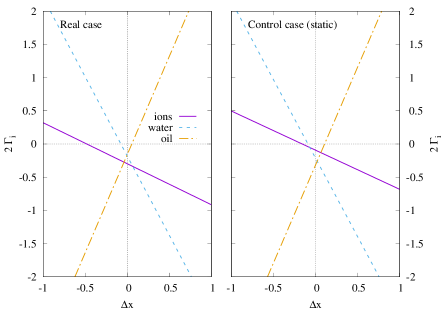
Figure 10: Interfacial excess for ions, water and oil as a function of the relative separation of the Gibbs dividing surfaces, for a concentration of ions of $20\%$. Left panel: real case, with dielectric mismatch; right panel: control (static) case, with no dielectric mismatch.

We do this first for the most concentrated ion solution (20%), and plot the resulting straight lines in Fig. 10 as a function of $\Delta x$, comparing the case where we have a dielectric discontinuity and a fully implemented polarisable water model (on the left) with a ‘control’ case where there is no dielectric discontinuity (on the right). We first note that there is no unique definition of $\Delta x$ which makes the water and oil interfacial excesses simultaneously vanish. This corresponds to the ‘dip’ in the total bead concentration seen in Fig. 9a. However, most striking is that the line for the ions lies below the intersection of the water and oil lines in the left hand plot, but above it in the right hand plot. This is a clear indication that ions are desorped from the interface in the case where there is a dielectric mismatch, compared to the control.

To further quantify this, let us define $\Delta x^{*}$ as the point where $\Gamma_{\text{water}}=0$ (i. e. where the dashed water lines in the plots cross the zero axis). We can then use this to define the relative surface excess for the ions $\Gamma_{\text{ions}}^{*}=\Gamma_{\text{ions}}(\Delta x^{*})$ Rowlinson and Widom (1989). This eliminates the dependence on $\Delta x$ and facilitates the propagation of errors in the calculation, however it is still arbitrary to some extent. Table 5 reports the results for a number of cases, clearly confirming ion desorption is significantly present only where there is a dielectric mismatch.

$c$ ($\%$)	$\Gamma_{\text{ions}}^{*}$	control (static)	control (polarisable)
5	$-$0.05(1)0	$-$0.007(8)	$-$0.015(4)
10	$-$0.088(7)	$-$0.013(9)	$-$0.026(8)
15	$-$0.107(8)	$-$0.02(1)0	$-$0.03(1)0
20	$-$0.125(8)	$-$0.020(9)	$-$0.05(1)0

Table 5: Ion surface excesses $\Gamma_{\text{ions}}^{*}$ relative to water (see text) as a function of the concentration in the water phase (total mole fraction of ions, as a percentage). Note desorption where there is dielectric mismatch (first column), compared to controls (second and third columns). This is further analysed in Table 6.

Finally, for the latter case, we define a (negative) adsorption length by dividing the surface excess by the bulk concentration in the water phase, $\Gamma_{\text{ions}}^{*}/\,{\overline{\rho}}_{\text{ions}}$ (we omit the superscript denoting the phase), and compare it to the Debye length $\lambda_{\text{D}}$ calculated from $\lambda_{\text{D}}^{-2}=4\pi l_{B}{\overline{\rho}}_{\text{ions}}$, being sure to use the Bjerrum length for water. Results are given in Table 6 mol . We see that the adsorption length is decreasing in magnitude as the concentration increases, and $\Gamma_{\text{ions}}^{*}/\,{\overline{\rho}}_{\text{ions}}\approx-\lambda_{\text{D}}/2$. This latter observation is a little puzzling, since we are in a concentration regime (see, e. g., second column in Table 6) where $\lambda_{\text{D}}$ should cease to have a physical meaning. Moreover, the adsorption length is smaller than the charge smearing length, and indeed likely smaller than the width of the interface itself (Fig. 9a). Further analysis is beyond the scope of the present study, but this is all highly intriguing and further work to explore this phenomenon is planned. We can also investigate the effect on the surface tension $\gamma$ itself gib .

$c$ (%)	$c/\mathrm{M}$	${\overline{\rho}}_{\text{ions}}$	$\Gamma_{\text{ions}}^{*}/\,{\overline{\rho}}_{\text{ions}}$	$\lambda_{\text{D}}$	$\Gamma_{\text{ions}}^{*}/(\lambda_{\text{D}}{\overline{\rho}}_{\text{ions}})$
05	0.5	0.158(2)	$-$0.33(9)	0.71(2)	$-$0.5(1)0
10	1.0	0.313(1)	$-$0.28(2)	0.50(1)	$-$0.56(6)
15	1.4	0.465(1)	$-$0.23(2)	0.41(1)	$-$0.55(6)
20	1.9	0.617(1)	$-$0.20(1)	0.359(9)	$-$0.56(5)

Table 6: Adsorption length for ions and the Debye length in the salt solution, and their ratio, for the dielectric mismatch case study (first column in Table 5). The second column indicates the approximate salt concentration in molar units, calculated using the length scale mapping in Sec. II.2.

V Water-in-vacuum models

We now return to a class of polarisable solvent models which use a vacuum as reference, thus $\epsilon_{b}=1$. These include the two Peter-Pivkin modelsPeter and Pivkin (2014); Peter et al. (2015), both of which are based upon the Drude oscillator water model developed for the MARTINI force field Yesylevskyy et al. (2010) and are equivalent to the dressed solvent model studied in this work with an additional bond angle potential. As we will discuss in the following, we believe these do not lead to the desired permittivity, therefore also we propose a third corrected version, which is an opportunity to demonstrate our approach to design a model with a desired permittivity. The three models are summarised in Table 7, together with a fourth trial one (see below).

		Ref. Peter and Pivkin,2014	Ref. Peter et al.,2015	***	†††
	$r_{c}$	$0.646\,\text{nm}$
	$A$	25
	$k_{d}/r_{c}^{-2}$	$10^{5}$
	$d_{0}/r_{c}$	0.2	0.2	0.5	0.5
	$k_{\theta}/\text{rad}^{-2}$	1	7.5	0	0
	$\theta_{0}$	0
	$q$	0.2	0.75	0.38	0.4
	$\lambda/r_{c}=1/\beta^{\star}$	0.7
	$l_{\text{B}}$	$55.0\,\text{nm}$
	$l_{\text{B}}/r_{c}$	85.9
	$\Gamma$ (coupling)	1080
	$\rho_{m}r_{c}^{3}$	3
MC	$\langle{\Delta{\bf r}^{2}}\rangle/r_{c}^{2}$	$4.08\times 10^{-2}$	$6.41\times 10^{-3}$	0.412	0.406
	$g_{\text{C}}$	1.06(2)	1.07(3)	1.20(3)	1.25(7)
	$\epsilon_{r}/\epsilon_{b}$	2.87(4)	5.1(1)	78(2)	89(5)
	$g_{\text{K}}$	0.83(2)	0.78(2)	0.80(2)	0.84(4)
Wert.	$\langle{\Delta{\bf r}^{2}}\rangle/r_{c}^{2}$	$4.24\times 10^{-2}$	$8.10\times 10^{-3}$	0.447	0.444
Ons.	$\epsilon_{r}/\epsilon_{b}$	3.39	7.94	104.9	115.7

Table 7: Parameters of Peter-Pivkin models designed for water relative to vacuum, and dielectric properties computed from Monte-Carlo simulations, compared to liquid state theory (cf. Table 2 and Table 3). The first two columns show parameters for the two published versions of the model. The third column (***) shows proposed parameters to recover the dielectric permittivity of water (in bold). Included for completeness, the fourth column (†††) is a trial (see text).

All the models were studied using the same techniques and codes as for the dimer and dressed solvent models, albeit with some modifications. While the dissipative particle dynamics (DPD) code in dl_meso required no modification, a reduction in time step size to $\delta t=0.001$ was needed to explicitly implement the stiff harmonic radial spring forces. The stiffness of these forces required a different approach from the standard Metropolis scheme for the Monte-Carlo (MC) code. In this case, we replace the radial springs by rigid arms of length $d_{0}$. These arms are free to rotate about the central bead, subject to the additional angular spring (which being soft causes no problems). To make a MC move with these rigid-arm trimers, we first select a bead or partial charge at random. If it is one of the solvent beads, we make a trial linear displacement of the whole molecule. If it is one of the partial charges we make a trial rotation of the arm, keeping the central bead and other arm fixed in position. The overall scheme is such that detailed balance is satisfied. No significant differences were observed between the DPD calculations with stiff harmonic bonds and MC calculations with rigid arms.

As shown in Table 7, the original Peter-Pivkin models proposed in Refs. Peter and Pivkin (2014) and Peter et al. (2015) have a dielectric permittivity which is nowhere near as large as reported, and we urge caution in using these models for aqueous systems, recommending alternative values for $d_{0}$ and $q$ to obtain the dielectric permittivity of water. Our confidence in these results is bolstered by the generally good alignment we find between the MC and dl_meso simulation results, and the Wertheim and Onsager theories applied to the present situation.

Given that the Bjerrum length is fixed by the choice of background (vacuum), the basic reason why the dielectric permittivity of the original models is too small in the original Peter-Pivkin models is that the dipole moment is too small. Our proposed remedy is therefore to increase the dipole moment, both by increasing the magnitude of the partial charges and lengthening the distance between them. If we limit ourselves to the case where the maximum separation between the partial charges $2d_{0}\leq r_{c}$, this suggests for maximum effectiveness the arm length $d_{0}=r_{c}/2$. We also propose to drop the angular potential as that can only have the effect of reducing the dipole moment. Then, we only have to adjust the magnitude of the partial charges to get the desired permittivity.

We start by injecting $\epsilon=78$ and $g_{\text{K}}=0.8$ into Eq. (12), and utilising the first of Eqs. (9) with $l_{\text{B}}/r_{c}=85.9$ and $\rho_{m}r_{c}^{3}=3$, to find we should target $q^{2}\langle{\Delta{\bf r}^{2}}\rangle\approx 0.0598\,r_{c}^{2}$. We cannot immediately deconvolute this since $q$ enters the plasma correction which affects the Wertheim theory prediction for $\langle{\Delta{\bf r}^{2}}\rangle$. However, one iteration here will suffice since the error will be corrected in the simulation stage. Starting from the simple analytic estimate $\langle{\Delta{\bf r}^{2}}\rangle=2d_{0}^{2}=0.5\,r_{c}^{2}$ from Appendix A, our initial guess is $q\approx 0.345$. We can now go back and incorporate the plasma correction in the Wertheim theory with this value of $q$. This improves the estimate to $\langle{\Delta{\bf r}^{2}}\rangle\approx 0.451\,r_{c}^{2}$, which now implies (first iteration) $q\approx 0.365$. Since we know this is unlikely to be exactly correct, let us round this up to $q=0.4$. If we simulate this (Table 7, final column), we find that $\epsilon\approx 89$ which is about 15% larger than what we want. Since we expect $\epsilon\propto q^{2}$ for $\epsilon\gg 1$ (Fig. 4a), we now adjust the magnitude of the partial charges to $q=0.38$ (rounding again). Checking this revised model, we find that its properties are (perhaps slightly fortuitously) exactly what we want (Table 7, third column).

This approach combines theoretical estimates using Wertheim and Onsager theory, with the assumption $g_{\text{K}}\approx 0.8$, to build an initial model which is then simulated to provide a concrete result with a single-step heuristic refinement. If we did not want to assume $g_{\text{K}}\approx 0.8$ in these models, we could also proceed by first supposing that $g_{\text{K}}=1$, and then measuring the dielectric permittivity and $g_{\text{C}}$ in the initial model to compute a better estimate for $g_{\text{K}}$ from Eq. (14), that could be fed back into the calculation. It seems likely that such a procedure should converge after at most one or two iterations.

VI Discussion

In this work we motivated the use of explicitly polarisable solvent models for mesoscale modelling of aqueous structured liquids, and interfaces in aqueous systems. We have examined two broad classes of such models, with applicability to the well-establised dissipative particle dynamics (DPD) mesoscale simulation methodology. For water in oil systems ($\epsilon_{r}/\epsilon_{b}\approx 40$) we propose a specific dressed DPD solvent model ‘WinO-DS’ (Table 2) which we confirm behaves as expected in a number of test situations, including capturing ion desorption from an oil-water interface. Amongst other interesting and worthwhile applications, such as the use of the model to explore ions at solvent interfaces, one can include the self assembly of ionic surfactants R. L. Anderson, et al. (2018), and the effect of a reduced dielectric permittivity in the micelle cores.

Our approach to design these solvent models has been to make sure that the partial charges are only weakly correlated on length scales $\gtrsim r_{c}$ (representing the solvent granularity), so that above this length scale the solvent appears as a uniform, featureless dielectric continuum. This motivates the use of molecular dipoles in which the separation of the partial charges is of the order $r_{c}$. Then, the magnitude $q$ of the partial charges is tuned as the final step to set $\epsilon_{r}/\epsilon_{b}$. In all the systems studied, the Kirkwood factor $g_{\text{K}}\approx 0.7$–0.8. If we assume that this holds true generally, then a good estimate of the system parameters needed to attain a target relative permittivity could be made via a combination of Wertheim and Onsager theory. This can be used as a starting point to iterate towards a final target value of the permittivity, with hopefully only a single calibration run required to fine-tune $q$ to get the desired ratio $\epsilon_{r}/\epsilon_{b}$. We therefore anticipate this approach is generically useful, for building mesoscale polarisable solvent models.

The models examined in the present work are all based on molecular dipoles with explicit (smeared) partial point charges. An intriguing opportunity exists though to make a polarisable solvent model in which true dipoles are embedded into DPD solvent beads. Most of the technical apparatus for this has already been developed. Ewald summation methods for computing forces and torques on dipoles S (98); Aguado and Madden (2003); Laino and Hutter (2008) can presumably be adapted to accommodate charge smearing; and likewise the necessary tools exist to deal with the rotational dynamics of the dipoles, and angular momentum conservation Müller et al. (2015). If such a solvent model is combined with many-body DPD Warren (2003), in principle one can simulate vapour-liquid interfaces with dielectric liquids, with possible applications for example to the electrical behaviour of nano-droplets in aerosols. We leave development along these lines for future work.

Appendix A Intramolecular potentials

We give details for the intramolecular potentials that can be used to calculate $\langle{\Delta{\bf r}^{2}}\rangle$ in Sec. III.5, for the models discussed in the main text. Recall $\beta\phi^{\text{int}}_{+-}(r)$ is the intramolecular potential between the partial charges separated by $r$ and arising from the bonded interactions, after integrating out all the other molecular degrees of freedom.

In the dimer class, there are no internal degrees of freedom and the intramolecular potential is trivially $\beta\phi^{\text{int}}_{+-}(r)=\frac{1}{2}k_{d}(r-d_{0})^{2}$, where we currently consider the case $d_{0}=0$. Note that unlike many molecular dynamics force fields Pronk et al. (2013), it is conventional in DPD modeling to retain the pairwise soft repulsions between all beads, including bonded pairs.

For the trimer class, one has to integrate out the central bead degrees of freedom. In general this leads to analytically intractable convolutions of Boltzmann factors, but conveniently for us analytic solutions can be given for the two specific models that we have focussed on in the present work. The first is the case where there are Hookean springs with $d_{0}=0$ and no angular potential. In that case the convolution also gives rise to an effective Hookean spring, with an effective spring constant which is the harmonic mean of the two original spring constants (Hookean springs in series), thus specifically in this case the effective spring constant is $k_{d}/2$ and the intramolecular potential $\beta\phi^{\text{int}}_{+-}(r)=k_{d}r^{2}/4$. For this, neglecting the plasma correction yields $\langle{\Delta{\bf r}^{2}}\rangle=3k_{\text{B}}T/(k_{d}/2)$.

The other case is the Peter-Pivkin model with rigid arms (of length $d_{0}$) where the only internal degree of freedom of the molecule is the opening angle $\theta$. Formally

$$4\pi r^{2}\exp[-\beta\phi^{\text{int}}_{+-}(r)]=\int_{0}^{\pi}\!\!\mathrm{d}\theta\;\frac{\sin\theta}{2}\,\exp[-{\textstyle\frac{1}{2}}k_{\theta}(\theta-\theta_{0})^{2}]\\ \times\delta(r-2d_{0}\sin{\textstyle\frac{1}{2}}\theta)\,.$$ (25)

The factors in the integrand are the density of states associated with the angular integration, the Boltzmann weight of the angular potential, and a $\delta$-function constraining the separation between the partial charges to $r$ (see Fig. 2b for geometry).

We make a change of variable to $u=2d_{0}\sin{\textstyle\frac{1}{2}}\theta$. The integral can now be done to get

$$4\pi r^{2}\exp[-\beta\phi^{\text{int}}_{+-}(r)]=\frac{r}{2d_{0}^{2}}\exp[-{\textstyle\frac{1}{2}}k_{\theta}(\theta-\theta_{0})^{2}]\,,$$ (26)

where $\theta=2\sin^{-1}(r/2d_{0})$. One application of this is to the case where there is no angular potential and the plasma correction is neglected. Then $4\pi r^{2}{\mathcal{P}}(r)=r/2d_{0}^{2}$ for $r\leq 2d_{0}$, and vanishes for $r>2d_{0}$, so that $\langle{\Delta{\bf r}^{2}}\rangle=\int_{0}^{2d_{0}}\!\mathrm{d}r\,r^{3}/2d_{0}^{2}=2d_{0}^{2}$.

Appendix B Charge smearing models

For completeness we report here details of the charge smearing models used in the simulations, and comment on the link to the Ewald method for dealing with electrostatics in periodic simulation boxes Frenkel and Smit (2002); Ibergay et al. (2009); Warren et al. (2013); Vaiwala et al. (2017). We also report in Table 8 some precision MC results for Slater charges as a benchmark for this problem. Excellent agreement is found with the HNC liquid state theory, with deviations only becoming apparent in the pressure for the largest $q$ value.

The Ewald method is based on the following summation identity Kittel (1956); Frenkel and Smit (2002)

$$\sum_{i>j}\frac{q_{i}q_{j}}{r_{ij}}=\frac{2\pi}{V}\sum_{k}A_{k}|Q_{\bf k}|^{2}+\sum_{i>j}\frac{q_{i}q_{j}}{r_{ij}}\operatorname{erfc}(\alpha r_{ij})\\ -\frac{\alpha}{\sqrt{\pi}}\sum_{i}q_{i}^{2}\,,$$ (27)

where $A_{k}=e^{-k^{2}/4\alpha^{2}}\!/k^{2}$ and $Q_{\bf k}=\sum_{i}q_{i}\,e^{-i{\bf k}\cdot{\bf r}_{i}}$. Here $\alpha$ is the Ewald ‘splitting parameter’.

For charge smeared models this becomes

$$\sum_{i>j}\frac{q_{i}q_{j}}{r_{ij}}[1-f(r_{ij})]=\frac{2\pi}{V}\sum_{k}A_{k}|Q_{\bf k}|^{2}\\ +\sum_{i>j}\frac{q_{i}q_{j}}{r_{ij}}[\operatorname{erfc}(\alpha r_{ij})-f(r_{ij})]-\frac{\alpha}{\sqrt{\pi}}\sum_{i}q_{i}^{2}\,,$$ (28)

where $f(r)=\operatorname{erfc}(r/2\sigma)$ for Gaussian charges Warren et al. (2013), and $f(r)=(1+\beta^{\star}r^{\star})e^{-2\beta^{\star}r^{\star}}$ for Slater smearing González-Melchor et al. (2006). We note the latter is an approximation for the interaction between Slater charges Warren and Vlasov (2014), but it is the one that is commonly used in the literature González-Melchor et al. (2006); Ibergay et al. (2009); Vaiwala et al. (2017). The three terms on the right hand side of Eq. (28) are the reciprocal space term, the real space term, and the self energy term. The last is a constant but should be retained to compare with HNC calculations of the energy density.

It is clear that choosing $2\alpha\sigma=1$ for Gaussian charges makes the real space term vanish Coslovich et al. (2011); Warren et al. (2013). This can be convenient albeit at the expense of losing the ability to tune $\alpha$ for computational efficiency Frenkel and Smit (2002). The final results should be insensitive to the choice of $\alpha$ (Table 8).

$q=0.2\>\to\>l_{\text{B}}q^{2}=3.436\,r_{c}$
	$\alpha$	$r_{\text{cut}}$	$k_{\text{cut}}$		${\mathfrak{p}}$	${\mathfrak{e}}$
HNC					$5.1262$	$-13.316$
MC	$0.75$	$3.0$	$4.5$		$5.12$	$-13.3$
	$1.0$	$3.0$	$5.5$		$5.13$	$-13.3$
$q=0.52\>\to\>l_{\text{B}}q^{2}=23.2274\,r_{c}$
	$\alpha$	$r_{\text{cut}}$	$k_{\text{cut}}$		${\mathfrak{p}}$	${\mathfrak{e}}$
HNC					$3.0266$	$-95.584$
MC	$0.75$	$3.0$	$4.5$		$3.03$	$-95.6$
	$1.0$	$3.0$	$5.5$		$3.04$	$-95.6$
$q=0.75\>\to\>l_{\text{B}}q^{2}=48.3188\,r_{c}$
	$\alpha$	$r_{\text{cut}}$	$k_{\text{cut}}$		${\mathfrak{p}}$	${\mathfrak{e}}$
HNC					$1.4927$	$-201.372$
MC	$0.75$	$3.0$	$4.5$		$1.69$	$-201.6$
	$1.0$	$3.0$	$5.5$		$1.67$	$-201.6$

Table 8: Precision Monte-Carlo (MC) results (dimensionless pressure ${\mathfrak{p}}$ and energy density ${\mathfrak{e}}$) supported by HNC calculations, for a Slater charge plasma under the stated conditions, with $l_{\text{B}}/r_{c}=85.9$ (coupling parameter $\Gamma=1080$), $A=0$, $\rho r_{c}^{3}=6$, $\lambda/r_{c}=1/\beta^{\star}=0.7$. MC results are reported with an estimated accuracy of 3 significant figures. The HNC pressure is the virial pressure.

The reciprocal and real space sums in Eq. (28) need cut-offs, $k_{\text{cut}}$ and $r_{\text{cut}}$ respectively, and care should be taken with this. For Slater charges with $1/\beta^{\star}=0.7$, examination of the real space contribution suggests $\alpha=1$ leads to the smallest $r_{\text{cut}}$, however this is a compromise since a larger $\alpha$ requires a larger $k_{\text{cut}}$ (essentially, this is controlled by the form of $A_{k}$).

The MC results in Table 8 were generated for two choices of $\alpha$, with the corresponding rather conservative choices for $k_{\text{cut}}$. All simulations were done with same real space cut-off $r_{\text{cut}}=3.0$ (in units of $r_{c}$) which is undoubtedly also rather conservative. Note that to use the minimum image convention in periodic boundary conditions the box size should be $\geq 2r_{\text{cut}}$ (the results in Table 8 were computed in an $8^{3}$ box). We note that the pressure is quite sensitive to $k_{\text{cut}}$ as a consequence of an extra factor $k^{2}$ in the reciprocal space contribution (see Eq. (12) in Ref. Warren et al. (2013)). The real space term contributes to the virial pressure in the usual way S (87).

Finally, we report the force law that derives from the above Ewald methodology. The general expression for the electrostatic force acting on particle $j$ due to reciprocal and real space contributions is

$$\begin{split}\frac{{\bf F}_{i}}{l_{\text{B}}q_{i}}&=-\frac{4\pi}{V}\sum_{k}i{\bf k}e^{-i{\bf k}\cdot{\bf r}_{i}}A_{k}Q_{\bf k}\\ &\hskip 20.00003pt{}+\sum_{j\neq i}\frac{q_{j}}{r_{ij}^{2}}\Bigl{[}\frac{2\alpha r_{ij}}{\sqrt{\pi}}e^{-\alpha^{2}r_{ij}^{2}}+\operatorname{erfc}(\alpha r_{ij})\\ &\hskip 80.00012pt{}+r_{ij}\,f^{\prime}\!(r_{ij})-f(r_{ij})\Bigr{]}\frac{{\bf r}_{ij}}{r_{ij}}\,,\end{split}$$ (29)

where $f^{\prime}\!(r)=df\!/dr$, and noting that no contribution arises from the self-energy term. As with the potential, the choice of $\alpha=1/(2\sigma)$ for Gaussian charges cancels out the real space force contribution. In the case of Slater charge smearing, the expression for the force is correctly given in Ref. Vaiwala et al. (2017). A previous expression for the force in the literature Ibergay et al. (2009) was based on the derivative of an incorrect form of the second (real space) term in Eq. (28): $\sum_{i>j}({q_{i}q_{j}}/{r_{ij}})\operatorname{erfc}\left(\alpha r_{ij}\right)\left[1-f(r_{ij})\right]$.

References

- Onsager and Samaras (1934) L. Onsager and N. N. T. Samaras, J. Chem. Phys. 2, 528 (1934).
- Bier et al. (2008) M. Bier, J. Zwanikken, and R. van Roij, Phys. Rev. Lett. 101, 046104 (2008).
- Frenkel and Smit (2002) D. Frenkel and B. Smit, Understanding Molecular Simulation (Academic Press, San Diego, CA, 2002).
- Español and Warren (2017) P. Español and P. B. Warren, J. Chem. Phys. 146, 150901 (2017).
- Fraaije et al. (2016) J. G. E. M. Fraaije, J. van Male, P. Becherer, and R. Serral Gracià, J. Chem. Inf. Model. 56, 2361 (2016).
- R. L. Anderson, et al. (2017) R. L. Anderson, et al., J. Chem. Phys. 147, 094503 (2017).
- Vishnyakov et al. (2013) A. Vishnyakov, M.-T. Lee, and A. V. Neimark, J. Phys. Chem. Lett. 4, 797 (2013).
- Lee et al. (2013) M.-T. Lee, A. Vishnyakov, and A. V. Neimark, J. Phys. Chem. B 117, 10304 (2013).
- M. A. Johnston, et al. (2016) M. A. Johnston, et al., J. Phys. Chem. B 120, 6337 (2016).
- R. L. Anderson, et al. (2018) R. L. Anderson, et al., J. Chem. Theory Comput. 14, 2633 (2018).
- Groot (2003a) R. D. Groot, J. Chem. Phys. 118, 11265 (2003a).
- Groot (2003b) R. D. Groot, J. Chem. Phys. 119, 10454 (2003b).
- Feynman et al. (1963) R. P. Feynman, R. B. Leighton, and M. Sands, The Feynman Lectures on Physics (Addison-Wesley, Reading, MA, 1963).
- Wertheim (1979) M. S. Wertheim, Ann. Rev. Phys. Chem. 30, 471 (1979).
- Stell et al. (1981) G. Stell, G. N. Patey, and J. S. Høye, Adv. Chem. Phys. 48, 183 (1981).
- Gray et al. (2011) C. G. Gray, K. E. Gubbins, and C. G. Joslin, Theory of Molecular Fluids, vol 2 (OUP, Oxford, UK, 2011).
- Allen and Tildesley (1987) M. P. Allen and D. J. Tildesley, Computer Simulation of Liquids (Clarendon, Oxford, UK, 1987).
- Groot and Warren (1997) R. D. Groot and P. B. Warren, J. Chem. Phys. 107, 4423 (1997).
- Peter and Pivkin (2014) E. K. Peter and I. V. Pivkin, J. Chem. Phys. 141, 164506 (2014).
- Peter et al. (2015) E. K. Peter, K. Lykov, and I. V. Pivkin, Phys. Chem. Chem. Phys. 17, 24452 (2015).
- Vaiwala et al. (2018) R. Vaiwala, S. Jadhav, and R. Thaokar, Mol. Sim. 44, 540 (2018).
- Yesylevskyy et al. (2010) S. O. Yesylevskyy, L. V. Schäfer, D. Sengupta, and S. J. Siewert J. Marrink, PLoS Comput. Biol. 6, e1000810 (2010).
- P. C. T. Souza, et al. (2021) P. C. T. Souza, et al., Nature Methods 18, 382 (2021).
- Groot and Rabone (2001) R. Groot and K. Rabone, Biophys. J. 81, 725 (2001).
- (25) With the exception of , we use subscripts to indicate permittivities which are defined relative to free space, and no subscript for permittivities defined relative to the static background.
- (26) The oil in this case would correspond to a non-polarisable liquid with so that its full permittivity is .
- Fisher and Ruelle (1966) M. E. Fisher and D. Ruelle, J. Math. Phys. 7, 260 (1966).
- Warren et al. (2013) P. B. Warren, A. Vlasov, L. Anton, and A. J. Masters, J. Chem. Phys. 138, 204907 (2013).
- Warren and Vlasov (2014) P. B. Warren and A. Vlasov, J. Chem. Phys. 140, 084904 (2014).
- González-Melchor et al. (2006) M. González-Melchor, E. Mayoral, M. E. Velázquez, and J. Alejandre, J. Chem. Phys. 125, 224107 (2006).
- Ibergay et al. (2009) C. Ibergay, P. Malfreyt, and D. J. Tildesley, J. Chem. Theory Comput. 5, 3245 (2009).
- Vaiwala et al. (2017) R. Vaiwala, S. Jadhav, and R. Thaokar, J. Chem. Phys. 146, 124904 (2017).
- Essmann et al. (1995) U. Essmann et al., J. Chem. Phys. 103, 8577 (1995).
- Seaton et al. (2013) M. A. Seaton, R. L. Anderson, S. Metz, and W. Smith, Mol. Simul. 39, 796 (2013).
- (35) Software utilities for dl_meso developed in the context of this work and the E-CAM project are available at https://e-cam.readthedocs.io/en/latest/Meso-Multi-Scale-Modelling-Modules/index.html. Note that the notation is slightly different from the present manuscript (please refer to the project documentation for details). For the present work, dl_meso v2.6 and the corresponding utilities were used.
- Hansen and McDonald (2006) J.-P. Hansen and I. R. McDonald, Theory of Simple Liquids (Academic Press, Amsterdam, The Netherlands, 2006).
- Kusalik et al. (1994) P. G. Kusalik, M. E. Mandy, and I. M. Svishchev, J. Chem. Phys. 100, 7654 (1994).
- (38) We use the subscript ‘box’ to distinguish this quantity from the polarisation density, introduced in Sec. IV.2.
- g (11) We have investigated the effect of the choice of boundary conditions on and plan to publish this separately.
- Böttcher (1973) C. J. F. Böttcher, Theory of Electric Polarization (Elsevier, Amsterdam, The Netherlands, 1973).
- (41) A. J. Masters et al., in preparation.
- (42) We use a pair of equal and opposite test charges, held fixed at a distance from each other along the diagonal of a (units ) simulation box.
- Keblinski et al. (2000) P. Keblinski, J. Eggebrecht, D. Wolf, and S. Phillpot, J. Chem. Phys. 113, 282 (2000).
- Rowlinson and Widom (1989) J. S. Rowlinson and B. Widom, Molecular Theory of Capillarity (OUP, Oxford, UK, 1989).
- (45) To obtain the molar concentrations, we divide the total ion density by , where the factor ‘2’ arises because each neutral ion pair contributes two ions, and is taken from Eq. (1).
- (46) In this context, if is the chemical potential of the -th species and is the pressure, the Gibbs-Duhem relation implies , since by mechanical force balance the pressures in the two phases are equal. This implies the Gibbs adsorption isotherm is independent of the choice of position of the Gibbs dividing surfaces, as is expected.
- S (98) W. Smith, CCP5 Newsletter No. 46 (1998).
- Aguado and Madden (2003) A. Aguado and P. A. Madden, J. Chem. Phys. 119, 7471 (2003).
- Laino and Hutter (2008) T. Laino and J. Hutter, J. Chem. Phys. 129, 074102 (2008).
- Müller et al. (2015) K. Müller, D. A. Fedosov, and G. Gompper, J. Comput. Phys. 281, 301 (2015).
- Warren (2003) P. B. Warren, Phys. Rev. E 68, 066702 (2003).
- Pronk et al. (2013) S. Pronk et al., Bioinformatics 29, 845 (2013).
- Kittel (1956) C. Kittel, Introduction to Solid State Physics, 2nd edn (Wiley, New York, NY, 1956).
- Coslovich et al. (2011) D. Coslovich, J.-P. Hansen, and G. Kahl, Soft Matter 7, 1690 (2011).
- S (87) W. Smith, CCP5 Newsletter No. 26 (1987).