Let It Flow: Simultaneous Optimization of 3D Flow and Object Clustering

Abstract

We study the problem of self-supervised 3D scene flow estimation from real large-scale raw point cloud sequences, which is crucial to various tasks like trajectory prediction or instance segmentation. In the absence of ground truth scene flow labels, contemporary approaches concentrate on deducing optimizing flow across sequential pairs of point clouds by incorporating structure based regularization on flow and object rigidity. The rigid objects are estimated by a variety of 3D spatial clustering methods. While state-of-the-art methods successfully capture overall scene motion using the Neural Prior structure, they encounter challenges in discerning multi-object motions. We identified the structural constraints and the use of large and strict rigid clusters as the main pitfall of the current approaches and we propose a novel clustering approach that allows for combination of overlapping soft clusters as well as non-overlapping rigid clusters representation. Flow is then jointly estimated with progressively growing non-overlapping rigid clusters together with fixed size overlapping soft clusters. We evaluate our method on multiple datasets with LiDAR point clouds, demonstrating the superior performance over the self-supervised baselines reaching new state of the art results. Our method especially excels in resolving flow in complicated dynamic scenes with multiple independently moving objects close to each other which includes pedestrians, cyclists and other vulnerable road users. Our codes will be publicly available.

Figure 1: Comparison of the proposed method with self-supervised competitors on Argoverse2 Dataset [3]. Our method is able to distinguish the different motion patterns and separate objects, while other methods tend to under-segment objects and fit incorrect rigid motion.

1 Introduction

Accurate estimation of the 3D flow field [13, 31, 19, 12] between two consecutive point cloud scans is crucial for many applications in autonomous driving and robotics as it provides per-point motion features inherently useful for a myriad of subsequent tasks, including semantic/instance segmentation [1, 33, 14], object detection [8, 14], motion prediction [22, 4, 15] or scene reconstruction [21]. Since manually annotated data for fully-supervised training are expensive and largely not available, we focus on the self-supervised setup, which is practically useful and reaches competitive results.

Self-supervision in 3D flow estimation always stems from strong prior assumptions about the scene structure. Many existing approaches, as exemplified by works [1, 11, 14, 19, 33], assume that the underlying scene consists of a static background and several rigid spatially compact objects, the motion of which satisfies kinematic and dynamic constraints. State-of-the-art methods [11, 19, 33, 7, 36] typically construct spatially compact clusters [9], that are assumed to correspond to rigidly moving objects as a first step and then apply rigid flow regularization for these clusters. Such premature clustering inevitably suffers from under-segmentation (i.e. merging several rigid objects into a single cluster) and over-segmentation (i.e. disintegration of a single rigid object to multiple clusters). To partially suppress the under-segmentation issue, the outlier rejection technique has recently been proposed [36]. Nevertheless, the quality of the initial clustering remains the main bottleneck, which prevents estimating the accurate flow, especially in situations where multiple small objects are moving independently close to each other. In contrast to existing approaches, we generate many small overlapping spatio-temporal rigid-cluster hypotheses and then jointly optimize the flow with the rigid-body segmentation. We quantitatively and qualitatively demonstrate that such an approach mitigates the over and under-segmentation issues and consequently yields superior results, especially on dynamic objects; see Figure 1 for the comparison.

Figure 2: Outline of the proposed losses: The left image shows pointcloud represented by black crosses that contains two vertical rigid objects. There is no spatial clustering that would segment them correctly; therefore any independent flow estimation will be strongly biased by the incorrect clustering. In contrast, we cover the pointcloud by (i) non-overlapping hard rigid clusters and (ii) overlapping soft rigid clusters. The right image demonstrates losses, visualized by springs, that are used for the flow estimation. The resulting flow is used for merging the hard clusters on spatio-temporal domain. The procedure is repeated until convergence. The resulting hard rigid clusters delivers rigid object segmentation.

In the proposed self-supervised framework, we employ two losses that are visualized using the analogy of a mechanical machine with springs, see Figure 2. The equilibrium of this machine corresponds to the globally optimal flow. The machine consists of two consecutive pointclouds in time (black and red crosses) which are not allowed to move, flow arrows attached to blue points by swivel telescopic joints, and two losses (rigid and distance) represented by springs. The scene depicts two rigid vertical objects that are moving in different directions. We employ standard distance loss (red springs), which attracts the flow of black points toward the corresponding red points from the consecutive pointcloud. Since objects in black pointcloud are close to each other, there is no spatial clustering that would separate them correctly. In contrast to existing methods, we instead introduce overlapping clusters (blue/green/magenta regions), within which the rigidity is encouraged through rigidity loss (blue/green/magenta springs). This rigid loss constructs springs among the arrow end-points in each source rigid-clusters, which prevents the flow from deforming the rigid cluster. The color of the springs matches the color of the cluster.

We also enable outlier rejection through spectral clustering as proposed in [36]. In terms of the mechanical machine analogy, the intuition of outlier rejection is that it adjusts the stiffness of springs in order to weaken the springs that connect outlier points (i.e. the points, the motion of which is non-rigid with respect to the rest of the cluster). To further regularize the flow, a structural regularization through Neural prior [20, 36, 21, 7] has also been proposed. We identified that the Neural prior regularizer helps mostly with static scenes flow estimation with a small number of dynamic objects; however, it over-regularizes the flow in highly dynamic scenes due to the limited capacity of the Neural-prior network. Therefore, we decided to drop this regularization in our proposed approach.

The main novelty of our approach stems from replacing the large spatially compact non-overlapping clusters delivered by an independent clustering algorithm, such as DBSCAN [9], with two different types of clusters: (i) soft mutually overlapping clusters, which are assumed to spread over multiple rigid objects and (ii) hard non-overlapping rigid clusters, which are expected to cover only the points from a single rigid object or its part. The soft clusters are optimized by the rigidity loss with outlier rejection, and the hard clusters are optimized by the rigidity loss without the outlier rejection. While soft clusters remain fixed, the hard clusters are progressively growing towards consistently moving points in the spatial and temporal domain.

We argue that while the flow estimated from large non-overlapping clusters [36] heavily suffers from over and under-segmentation, usage of the proposed overlapping growing clusters significantly suppresses this issue, see Figure 1. In particular, it mitigates the over-segmentation by spatially propagating the rigidity through the overlap; see Figure 2, for example, that the blue and magenta clusters deliver strong rigidity springs between the points of the left object, which consequently grows the hard rigid cluster over the whole rigid object. Mitigation of the under-segmentation is achieved by using only small rigid clusters combined with outlier rejection techniques; for example, even though all three soft clusters contain an outlier, the resulting rigidity springs between left and right rigid objects are weakened, and the hard rigid cluster grows only within the rigid object. Consequently, the only assumption required in order to correctly segment inconsistently moving rigid objects is that each point of the rigid object appears as an inlier in at least one soft cluster hypothesis.

The main contributions of the paper are three-fold:

• Novel clustering method, where the rigid object segmentation is initialized from spatial-temporal grouping and is jointly optimized with the flow.

• The proposed self-supervised method achieves superior accuracy among state-of-the-art methods [21, 7, 20, 17] on all tested datasets (Agroverse2 [3], Waymo [34], StereoKITTI [27])

• Significant improvements on long tail classes, such as independently moving pedestrians and cyclists, where current solutions fail due to structural prior regularization.

2 Related Work

Supervised scene flow.

In the early stages of learning-based 3D scene flow estimation, methodologies relied on synthetic datasets [12, 26, 38, 25] for preliminary training. FlowNet3D [24], assimilated principles from FlowNet [13] and underwent comprehensive supervised training, employing L2 loss in conjunction with ground-truth flow annotations. BiPFN [6] orchestrated the bidirectional propagation of features from each point cloud, thereby enriching the representation of individual points. FLOT [31] introduced an innovative correspondence-based network, transforming the initial flow estimation to optimal transport estimation problem, succeeded by meticulous flow refinement through trained convolutions. The recently unveiled IHNet architecture [39] proposes an iterative hierarchical network, steered by high-resolution inferred information and estimating flow in a coarse-to-fine manner.

Self-supervised scene flow.

Recent methodologies have sidestepped the requirement for ground-truth flow by embracing self-supervised learning. Among the early adopters of this approach, PointPWC-Net [41] presented a wholly self-supervised methodology, combining nearest-neighbors and Laplacian losses. Similarly, in [28], a self-supervised nearest neighbor loss was implemented, ensuring the cycle consistency between forward and reverse scene flow. Najibi et al. [29] employ self-learned flow within an automated pseudo-labeling pipeline, designed for training an open-set object detector and trajectory predictor. RigidFlow [19] formulates a methodology for generating pseudo scene flow within the domain of self-supervised learning. This approach relies on piecewise rigid motion estimation applied to collections of pseudo-rigid regions, identified through the supervoxels method [23]. Flowstep3D [16] undertakes flow estimation through local and global feature matching utilizing correlation matrices and iterative warping. The method known as SCOOP [17] adopts a hybrid framework of correspondence-based feature matching, coupled with a flow refinement layer employing self-supervised losses. Shen et al. [32] seamlessly integrated superpoint generation directly into their model for iterative flow refinement. Compared to supervised and self-supervised approaches, our method do not require any labeled or unlabeled training data as it is optimization-based.

Direct flow optimization.

The Graph Prior approach, as introduced by [30], is rooted in pure optimization, enabling flow estimation without the need for training data. The Neural Prior[20] illustrates that flows can be optimized by incorporating a structure-based prior within the network architecture. The central objective in [21] revolves around expediting the Neural Scene Flow [21]. Li et al. identify the Chamfer distance as a computational bottleneck and use the Distance Transform as a surrogate correspondence-free loss function. The methodology outlined in Scene Flow via Distillation by [35] embodies a direct distillation framework. This innovative approach utilizes a label-free optimization method to generate pseudo-labels, which are subsequently employed to supervise a feed-forward model to achieve better speed/performance ratio. The two newest optimization-based methods, the MBNSFP [36] and Chodosh [7] adopt Neural Prior architecture and enhanced it with spatial consistency regularization [36] and post-process cluster rigidity [7], respectively. We also use rigidity regularization, but we do not limit our method to fixed initial clusters as [36, 7]. Instead, we jointly optimize initial cluster and flow to progressively merge and enlarge clusters while enforcing rigidity on them. Another difference to aforementioned methods, is the absence of Neural Prior as structural regularization, which plays crucial role for populated dynamic scenes.

Rigidity Regularization.

Given the presence of multiple local minima in the conventional self-supervised Chamfer distance loss, the introduction of regularization mechanisms becomes imperative to attain physically plausible flows—ones that faithfully trace the motion of rigid structures and objects. Implicit rigidity regularization is enforced through a robust model prior in [20, 2, 42]. The introduction of weak supervision, in the form of ego-motion and foreground segmentation, has demonstrated its capacity to provide object-level abstraction for estimating rigid flows [11]. FlowStep3D [16] imposed constraints on the source point cloud to preserve its Laplacian when warped by the predicted flow, constituting the smoothness loss. SLIM [1] incorporated the smoothness loss into the process of learning network weights and SCOOP [17] integrated the smoothness loss within the optimization-based flow refinement layer. In [5], a novel global similarity measure takes the form of a second-order spatial compatibility measure on consensus seeds, that serve as input to a weighted SVD algorithm, ultimately producing global rigid transformation. Contrary to [5], we use spatial consistency mechanism for rigidity regularization, but for multiple objects.

3 Method

The main goal is the self-supervised estimation of the flow field $F$ between two consecutive point clouds $P$ and $Q$. Point clouds consist of 3D points $\mathbf{p}_{i}\in P\subset\mathbb{R}^{3}$ and $\mathbf{q}_{i}\in Q\subset\mathbb{R}^{3}$. Since real-world scenes consist mostly of a static background, we follow a good practice of compensating the ego-motion [7] first before running our method. We calculate the ICP [37] as an estimate of ego-motion and use it to transform the source point cloud $P$. In the rest of this section, we focus on the estimation of the remaining flow, which corresponds to the motion between transformed source pointcloud $P$ and target pointcloud $Q$. Consequently, the flow of point $\mathbf{p}_{i}\in P$ is a 3D vector $\mathbf{f}_{i}\in F\subset\mathbb{R}^{3}$ that is non-zero only on dynamic objects if the ego-motion is correctly estimated.

3.1 Method overview

The method is summarized by pseudo-code in Algorithm 1. The proposed method first initialize two sets of clusters: hard and soft. Hard rigid clusters are non-overlapping small clusters that are assumed to cover only a single rigid object or its part. Each rigid cluster $H\in\mathcal{H}$ is a small compact cluster delivered through spatial-temporal segmentation on $P$ including the adjacent temporal point clouds. In contrast, the soft rigid clusters are small overlapping clusters that are expected to overflow into neighboring objects. Each point $\mathbf{p}\in P$ is associated with the one soft cluster $S\in\mathcal{S}$, which is defined as the set of its $k$ nearest neighbours $N_{k}(\mathbf{p},P)$ from the pointcloud $P$. Given these two sets of clusters, we optimize the flow to minimize (i) hard rigidity loss on hard clusters, (ii) soft rigidity loss on soft clusters and (iii) distance loss on all points. Both rigidity losses enforce rigid flow on points within the cluster. The main difference is that the soft rigidity loss allows for outlier rejection. All losses are detailed in the following paragraphs. Once the optimized flow is available, we merge rigid clusters in $P$, whose flow goes into the same rigid cluster in $Q$. Since the algorithm is iteratively called on all consecutive pairs of pointclouds, the rigidity is propagated throughout the temporal domain.

Algorithm 1 Joint flow estimation and rigid object segmentation

pointcloud $P,Q$

flow $F$

1. Initialize set of hard rigid clusters $\mathcal{H}$.

2. Initialize set of soft rigid clusters $\mathcal{S}$.

3. Optimize

   $$\mathcal{L}(F)=\alpha\sum_{\mathbf{f}\in F}\mathcal{L}_{\textrm{dist}}(\mathbf{f})+\beta\sum_{H\in\mathcal{H}}\sum_{\mathbf{f}\in H}\mathcal{L}_{\textrm{hard}}(\mathbf{f})+\gamma\sum_{S\in\mathcal{S}}\sum_{\mathbf{f}\in S}\mathcal{L}_{\textrm{soft}}(\mathbf{f}),$$

   where $\alpha,\beta$ and $\gamma$ are hyper-parameters of the proposed method.

4. If the flow of two different rigid clusters $H_{i},H_{j}\in\mathcal{H}$ goes into the same rigid cluster in pointcloud $Q$, then merge $H_{i},H_{j}$ into the same cluster.

5. Repeat from 3 until convergence or reaching maximum number of iterations.

3.2 Distance loss

Similarly to existing approaches, we assume that the motion of objects is sufficiently small with respect to the spatio-temporal resolution of the sensor. This assumption transforms into so-called distance loss, which attracts the flow of points from the point cloud $P$ toward the consecutive point cloud $Q$.

$$\mathcal{L}_{\mathrm{dist}}(\mathbf{f})=\sum_{i\in P}\|\mathbf{p}_{i}+\mathbf{f}_{i}-N_{1}(\mathbf{p}_{i}+\mathbf{f}_{i},Q)\|$$ (1)

where $N_{1}(\mathbf{p},Q)$ is the nearest neighbour of point $\mathbf{p}$ from pointcloud $Q$. In practice, we use it bidirectionally for both point sets $P,Q$, which is equivalent to Chamfer distance.

3.3 Hard rigidity loss

Since the distance loss is typically insufficient for a reliable flow estimation, the additional prior assumption that takes into account the rigidity of objects is considered. In contrast to existing approaches [9, 11, 33, 36], we do not explicitly model a fixed number of independently moving rigid objects, but we simultaneously optimize flow with the rigid clusters as describe in Algorithm 1. Given a cluster $C$ consisting of $k$ points from pointcloud $P$, we construct the complete undirected graph $\mathcal{G}=(\mathcal{V},\mathcal{E})$ with $k$ vertices $\mathcal{V}=C$ and $k(k-1)/2$ edges $\mathcal{E}$ corresponding to all possible pair-wise connections among points (without self-loops). Each edge is associated with a reward function that encourages the flow in incident vertices to preserve the mutual distance between the corresponding points, i.e., encourage the rigid motion. The reward for preserving rigidity is defined as follows:

$$r_{ij}=1-\sum_{u}\frac{(d_{ij}^{u}-\hat{d}_{ij}^{u})^{2}}{\theta},$$ (2)

where $d_{ij}^{u}=|\mathbf{p}_{i}^{u}-\mathbf{p}_{j}^{u}|$ is the distance between the $u$-th dimension of points $\mathbf{p}_{i},\mathbf{p}_{j}\in C$ and similarly $\hat{d}_{ij}^{u}=|(\mathbf{p}_{i}^{u}+\mathbf{f}_{i}^{u})-(\mathbf{p}_{j}^{u}+\mathbf{f}_{j}^{u})|$ is the distance after applying the estimated flow on these points, and $\theta$ is a hyper-parameter of the proposed method. If the motion is rigid, the distance difference is zero, and the reward equals one; if the distance is non-zero the reward is proportionally smaller. Given this notation, we introduce hard rigidity loss

$$\mathcal{L}_{\textrm{hard}}(\mathbf{f})=\sum_{(\mathbf{p}_{i},\mathbf{p}_{j})\in\mathcal{V}}-\log(r_{ij}).$$ (3)

3.4 Soft rigidity loss

Intuitively, when the cluster $C$ is incorrect (e.g. it overflows into neighbouring objects), the optimization of the flow through the hard rigid loss delivers inaccurate flow. In order to enable outlier rejection, we introduce $k$-dimensional soft clustering vector $\mathbf{v}\in\mathopen{[}0,1\mathclose{]}^{(k+1)},\|\mathbf{v}\|=1$ that is supposed to softly selects high-reward edges. This vector models how much the points are likely to be in the rigid object that is dominant within the cluster. Given this notation, we define the soft rigidity score induced by the point $\mathbf{p}_{m}$ as

$$s_{m}(\mathbf{v})=\sum_{(\mathbf{p}_{i},\mathbf{p}_{j})\in\mathcal{V}}r_{ij}\mathbf{v}_{i}\mathbf{v}_{j}=\mathbf{v}^{\top}\mathbf{A}_{m}\mathbf{v},$$ (4)

where matrix $\mathbf{A}_{m}$ consists of elements $[\mathbf{A}_{m}]_{i,j}=r_{ij}$. Product $\mathbf{v}_{i}\mathbf{v}_{j}$ corresponds to the spring stiffness between point $\mathbf{p}_{i}$ and $\mathbf{p}_{j}$ in the mechanical analogy from Figure 1.

Given the score matrix $\mathbf{A}_{m}$, the optimal soft clustering is, by Raleigh’s ratio theorem, the principal eigenvector of matrix $\mathbf{A}_{m}$

$$\mathrm{eig}(\mathbf{A}_{m})=\mathop{\arg\max}_{\|\mathbf{v}\|=1}\mathbf{v}^{\top}\mathbf{A}_{m}\mathbf{v}.$$ (5)

The score (4) for the optimal soft clustering (which is equal to the principal eigenvalue of $\mathbf{A}_{m}$) describes how much the flow is consistent with the rigid motion. In order to make the estimated flow more rigid under the optimal soft clustering, we introduce the soft rigidity loss

$$\mathcal{L}_{\textrm{soft}}(\mathbf{f})=\sum_{m}-\log\Big{(}s_{m}\big{(}\mathrm{eig}(\mathbf{A}_{m}(\mathbf{f}))\big{)}\Big{)},$$ (6)

which pushes the principal eigenvalue up and consequently makes the flow on spatially compact clusters more rigid.

4 Experiments

Datasets.

We conducted experiments using standard scene flow benchmarks. Firstly, we employed two large-scale, well-known LiDAR autonomous driving datasets: Argoverse1 [3] and also newer version Argoverse2 [40] and Waymo [34] open dataset. These datasets encompass challenging dynamic scenes with various maneuvers captured by different LiDAR sensor suites. To ensure a fair comparison, we sampled and processed the LiDAR datasets according to the methodology outlined in [20] and use validation split sequences first frames. As there are no official scene flow annotations, we adopted the data processing approach from [15] to derive pseudo-ground-truth scene flow information based on object detection annotations, akin to the methodology employed in [20]. Finally, we removed ground points in the height of 0.3 meters or lower for Waymo dataset, following the procedure outlined in previous works [24, 20, 17, 21, 11, 36]. For Argoverse1 and Argoverse2, we used the accompanying ground maps to remove ground points and constrain the range of input points to 35 meters as done in [7, 11, 41, 17].

Subsequently, we utilized the stereoKITTI dataset [27, 24], which comprises real-world scenes from autonomous driving scenarios. The point clouds in the stereoKITTI dataset are however constructed by lifting the depth from stereo images by calculated optical flow, resulting in 3D points with one-to-one correspondence and huge amount of dynamic points per object [7]. The dataset was further divided by [28] into a testing part referred to as KITTI_t.

Implementation Details.

We use $k=16$ and set $\alpha$ and $\beta$ loss weights to 1. We use the learning rate of 0.004. The $\theta$ distance threshold for outlier rejection is set to 0.03 as in [5, 36]. We perform hard clustering by spatio-temporal DBSCAN over horizon of 5 point clouds and set epsilon parameter to 0.3 and minimal samples to 1, resulting in clustering the points to the same cluster if the Euclidian distance is lower than 0.3. The flows are optimized until a fixed number of iterations (1500) or until reaching the convergence of the loss function. For other comparative methods, we use the same optimized parameters as reported in their original papers and official implementations.

Evaluation metrics.

For proper evaluation of results we need to define point error $e_{i}$ and relative point error $e_{i}^{r}$. Following the notation introduced in Section 3, we define these errors in meters as follows:

$$e_{i}=\|\mathbf{f}_{i}-\mathbf{f}^{\text{gt}}_{i}\|_{2},\quad e^{\text{r}}_{i}=\frac{{\|\mathbf{f}_{i}-\mathbf{f}^{\text{gt}}_{i}\|}_{2}}{\|\mathbf{f}^{\text{gt}}_{i}\|_{2}},$$

where $\mathbf{f}_{i}$ and $\mathbf{f}^{\text{gt}}_{i}$ are the predicted and ground-truth flow for point $\mathbf{p}_{i}$, respectively. From $e_{i},e^{\text{r}}$ we calculate Average Point Error in meters (EPE), Strict Accuracy (AS), Relaxed Accuracy (AR), Angle Error ($\theta$) and Outliers ($Out.$), which are standard metrics used in the literature, e.g., [20, 17]. AS is a percentage of points that reached errors $e_{i}<0.05$ or $e^{\text{r}}_{i}<5\%$. The AR is the percentage of points for which the error satisfies either $e_{i}<0.1$ or $e^{\text{r}}_{i}<10\%$. Metric $Out.$ is the percentage of points with error either $e_{i}>0.3$ or $e^{\text{r}}_{i}>10\%$, and finally $\theta$ denotes the mean angle error between $\mathbf{f}_{i}$ and $\mathbf{f}^{\text{gt}}_{i}$.

In automotive scenes, the majority of the points come from a static background. When the metrics ($EPE$, $AS$, $AR$) are calculated and averaged for the full point cloud, the results show mostly performance on static points, lowering the importance of dynamic objects [7, 35]. If we dig even further, the dynamic points are heavily dominated by large vehicles and the performance on smaller, yet equally important classes, like Pedestrians and Cyclists are not observable from the dynamic $EPE$ metrics. Therefore, we also report the metrics per-class on the main benchmark, Argoverse2.

4.1 Comparison with State-of-the-Art Methods

Table 1: Performance on Argoverse2 dataset in foreground aware metrics, i.e. Threeway EPE metric.

		Dynamic Foreground			Static Foreground			Static Background
Methods	Avg. EPE [m]$\downarrow$	EPE [m]$\downarrow$	AS [%]$\uparrow$	AR [%]$\uparrow$	EPE [m]$\downarrow$	AS [%]$\uparrow$	AR [%]$\uparrow$	EPE [m]$\downarrow$	AS [%]$\uparrow$	AR [%]$\uparrow$
MBNSFP [36]	0.159	0.393	9.325	25.72	0.034	88.54	96.98	0.051	84.96	92.59
NSFP [20]	0.083	0.141	39.85	71.69	0.059	75.15	91.14	0.048	81.96	93.56
Chodosh [7]	0.070	0.132	41.80	75.49	0.049	77.29	93.74	0.028	87.97	95.30
Ours	0.047	0.079	67.90	85.35	0.035	86.26	95.78	0.026	93.02	96.30

Table 2: Performance on Argoverse2 dataset in object class aware EPE.

	Pedestrian			Cyclist			Vehicles
Methods	Avg.$\downarrow$	Dyn.$\downarrow$	Stat.$\downarrow$	Avg.$\downarrow$	Dyn.$\downarrow$	Stat.$\downarrow$	Avg.$\downarrow$	Dyn.$\downarrow$	Stat.$\downarrow$
MBNSFP [36]	0.071	0.115	0.026	0.302	0.570	0.034	0.245	0.457	0.034
NSFP [20]	0.062	0.080	0.044	0.058	0.099	0.017	0.111	0.156	0.065
Chodosh [7]	0.068	0.083	0.052	0.047	0.083	0.011	0.100	0.145	0.054
Ours	0.031	0.039	0.023	0.012	0.016	0.009	0.068	0.097	0.039

We benchmark our method against the top-performing methods, such as NSFP [20], MBNSFP [36] and Chodosh [14], which all share the same structural optimization-based regularization, i.e Neural Prior [20, 21]. For all methods, we use the official implementation provided in papers. For Chodosh [7], we used the codebase published in [35]. For each method, we compensate the ego-motion with KISS-ICP [37] first, then estimate the flow by methods.

In Table 1, we show results on Argoverse2, the main benchmark for 3D scene flow estimation. Our method dominates the dynamic foreground metrics, while the MBNSFP [36] has better static foreground. We suggest, that their reliance on Neural prior architecture coupled with under-segmented rigidity tends to overfit on the static classes, since they share a single movement, caused by ego-motion, and the MLP layers in Neural Prior do not have expressive capacity to catch multiple motion patterns. Chodosh [7] do not optimize rigidity and Neural prior jointly, but fine-tune the rigidity as a post-processing step, resulting in more separable object motion. Our method without Neural Prior and merging clusters achieves the best average EPE over the dynamic and static metrics.

When zooming in to per-class scene flows, we observe a trend of overfitting to larger dynamic objects, i.e. vehicles. We suggest, that fitting one structural neural prior to multiple objects in the scene leads to the local minima of solving the objects with the most of points, and sacrificing the smaller ones. In Table 2, we show the performance on Pedestrians, Cyclists and Vehicles separately. For example, we can see, that the performance of the other methods on Pedestrian class is halved, compared to ours, where the over-segmentation of the scene usually safely cluster the whole Pedestrian as one hard cluster and estimate rigid flow without structural neural constraints. We see that in Cyclist category, the performance of ours is even higher. We do not lose the ability estimate flows on Vehicles, as we can separate them in our merging clustering as well. We have worse static vehicles compared to MBNSFP[36], which we explain by overfitting into static flow.

4.2 Neural Prior with Hard and Soft Clusters.

In order to compare our proposed rigidity via hard and soft clusters to the most similar methods (MBNSFP [36] as it also use spatial consistency with outlier rejection), we change the direct optimization of flows for neural prior architecture as in other methods [20, 36, 7]. We also perform experiments under the metrics proposed in MBNSFP [36], i.e. overall end point error without foreground/background split.

In Table 3, we see the results on Waymo [34] and Argoverse1 [3] datasets on splits used in  [36]. We can see, that the better performance is reached with our rigidity regularization. The MBNSFP [36] is the second top-performing methods with regular Neural prior [20] with cycle consistency and structural regularization behind.

Runtime Benefit of Implementing Soft Clusters as Neighborhoods.

We analyze the performance-time trade-off in Figure 3 by acquiring the $EPE$ based on inference time for our method on Argoverse1 dataset while using Neural Prior architecture with proposed Soft Clusters. The speed was measured on NVIDIA Tesla V100 GPU on complete point clouds. We compare with optimization-based methods FastNSF [21] and MBNSF [36] with distance transform acceleration proposed by [21] and DBSCAN clustering, and Neural prior [20] without distance transform acceleration [21].

Table 3: Performance on LiDAR datasets. We show performance on standard LiDAR benchmarks with overall metrics (without dynamic/class split). Results are averages over 3 runs.

Dataset	Method	EPE [m]$\downarrow$	AS [%]$\uparrow$	AR [%]$\uparrow$	$\theta$ [rad]$\downarrow$
	JGF [28]	0.542	8.80	20.28	0.715
	PointPWC-Net [41]	0.409	9.79	29.31	0.643
Argoverse1	NSFP	0.065	77.89	90.68	0.230
	MBNSFP [36]	0.057	86.76	92.46	0.273
	NSFP + Ours	0.050	87.06	94.26	0.269
	R3DSF[11]	0.414	35.47	44.96	0.527
	NSFP[20]	0.087	78.96	89.96	0.300
Waymo	MBNSFP[36]	0.066	82.29	92.44	0.277
	NSFP + Ours	0.039	88.96	95.65	0.297

Compared to the MBNSFP [36], our method is approximately $\mathbf{10}\times$ faster while stopping at the same prediction error. Even though their spatial consistency regularization uses the same algorithm of computing the point-to-point displacements with outlier rejection, our method is significantly faster because we design the clusters on the same-sized neighborhoods, which can be efficiently parallelized on GPUs. In contrast to our method, MBNSFP computes eigen vectors of matrix with variable-sized clusters [9]. Thus, MBNSFP is looping over $c$ clusters $\{N_{0},N_{1},...,N_{c}\}$ one-by-one, whereas our method allows GPU to parallel the $\mathbb{R}^{N\times k\times k}$ tensor computation for $N$ points in point cloud and $k$ neighbors simultaneously.

Figure 3: Flow estimation error vs. run time on Argoverse1 dataset. Our method in green offers speed-accuracy trade-off that outperforms the converged baselines on overall EPE metric.

4.3 Results on StereoKITTI benchmark.

We also evaluate our method on both the full StereoKITTI and its testing subset KITTI_t  following the experimental setting in [17, 28, 16]. We compare our method to the top-performing methods in self-supervised 3D scene flow and also to recent fully-supervised methods trained on FT3D [10] dataset. Our self-supervised method without any training data is on par with the most recent and top performing fully-supervised method, the IHNet [39] in terms of $AS$ (Ours 98.0% and fully-supervised IHNet 97.8%), see Figure 4.

Our main baselines for performance comparison are state of the art self-supervised methods such as SCOOP [17], SLIM [1], FastNSF [21], Rigid Flow [19]. Our method achieves the new self-supervised state-of-the-art performance on stereoKITTI benchmark with the relative improvement of 38% of $EPE$ compared to top-performing SCOOP [17] on StereoKITTI and also achieves the improvement of 42% of $EPE$ compared to the top-performing NSFP [21] on KITTI_t.

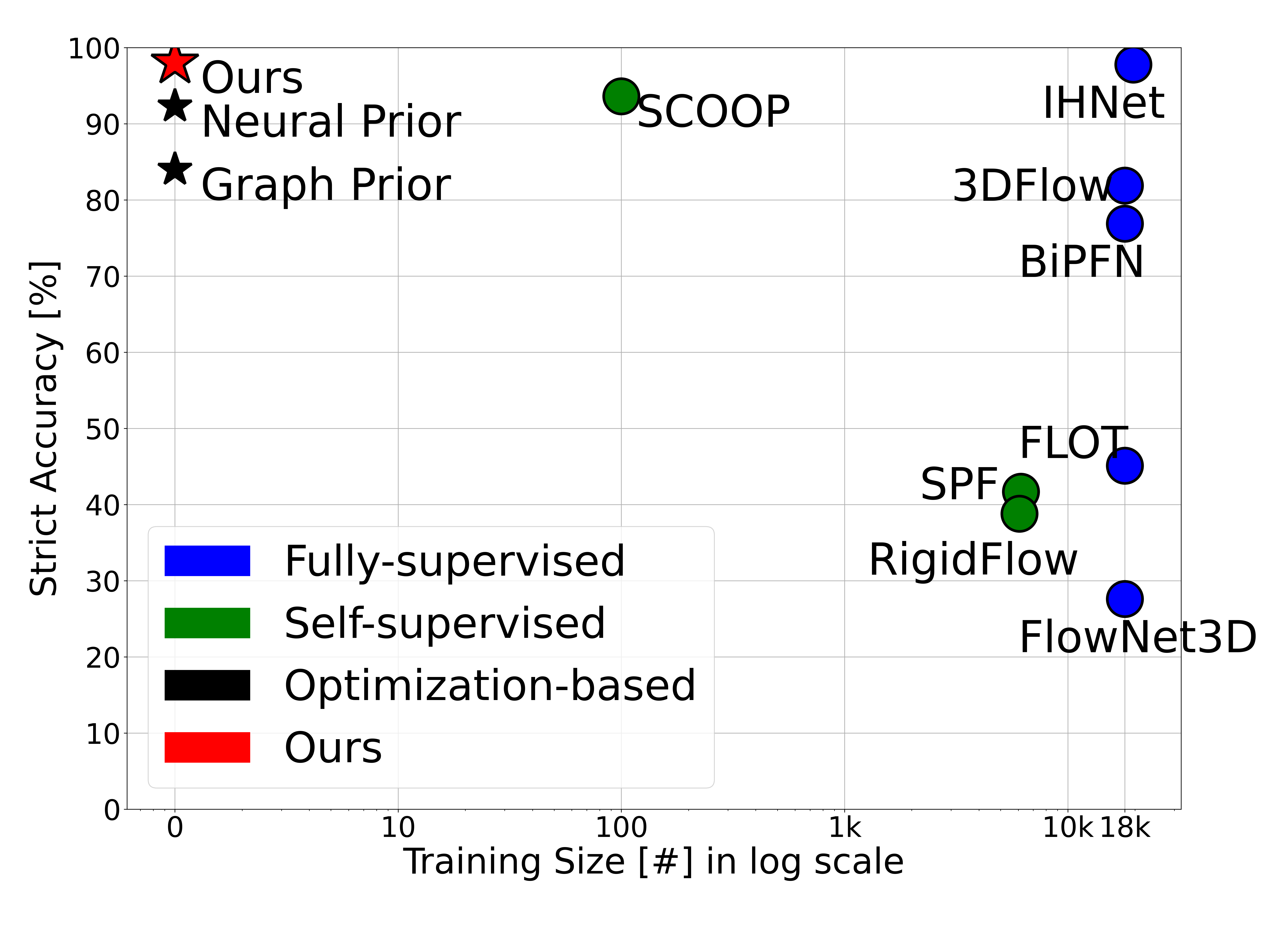
Figure 4: Comparison of the proposed method with self-supervised [17, 19, 18, 20, 30] and fully-supervised [24, 31, 39] competitors on StereoKITTI benchmark.

Table 4: Comparison with State-of-the-Art on KITTI dataset. We evaluate scene flow based on standard metrics $EPE$, $AS$, $AR$ and $Out.$ for StereoKITTI dataset. Previous state of the art performance is underlined and current best is in bold. Our results averaged over 5 runs.

Test data	Method	$EPE(m)$ $\downarrow$	$AS(\%)$ $\uparrow$	$AR(\%)$ $\uparrow$	$Out.(\%)$ $\downarrow$
KITTIo	FlowStep3D [16]	0.102	70.8	83.9	24.6
	RigidFlow [19]	0.102	48.4	75.6	44.2
	SLIM [1]	0.067	77.0	93.4	24.9
	MBNSFP [36]	0.112	80.7	86.3	14.5
	NSFP [21]	0.051	89.8	95.1	14.3
	SCOOP [17]	0.047	91.3	95.0	18.6
	Ours	0.029	98.0	98.7	11.7
KITTIt	JGF [28]	0.105	46.5	79.4	-
	RigidFlow [19]	0.117	38.8	69.7	-
	MBNSFP [36]	0.112	81.6	87.3	15.0
	SCOOP [17]	0.039	93.6	96.5	15.2
	NSFP [21]	0.036	92.3	96.2	13.2
	Ours	0.021	98.7	99.1	11.0

4.4 Ablation Study

Method components

In Table 5, we show metrics when adding one enhancement per time. We observe the benefits of components on final performance on the Argoverse2 dataset. Without rigidity regularization and clusters a), the methods resembles flow only to the nearest neighbors in target point cloud and therefore fails to produce meaningful motions. By including the hard cluster rigidity b), we observe physically consistent motions. However, since we enforce rigidity on over-segmented clusters, the objects still deforms. With addition of soft clusters c), we are able to connect nearby points from different hard segments to rigidity term and reject outliers, expanding the object rigidity. By guiding the hard clusterization with flows d), we acquire small boost by connecting lonely clusters divided by occlusions or separate by LiDAR sampling rate back to the major rigid body.

Table 5: Ablation study for individual method components on Argoverse2.

Module	Avg. $EPE(m)$ $\downarrow$	Dyn. Fore. $EPE(m)$ $\downarrow$	Stat. Fore. $EPE(m)$ $\downarrow$	Stat. Back. $EPE(m)$ $\downarrow$
a) w/o Rigidity	0.244	0.504	0.103	0.124
b) w/ Hard Clusters Rigidity	0.052	0.089	0.040	0.028
c) w/ Hard Clusters and Soft Clusters Rigidity	0.047	0.079	0.035	0.026
d) w/ Rigidity and Flow Guided Hard Clusters	0.046	0.077	0.035	0.025

5 Limitations

Even though our method is reasonably fast, it still does not, as the other methods, achieve real-time performance while keeping high accuracy. Potential direction for improvement is shown in [35]. Secondly, our method does not deal with the local minima of the distance loss, resulting in sub-optimal flows even when the object is correctly clustered. These two issues are worth of the future research to improve scene flow further.

6 Conclusion

We presented a novel self-supervised method for 3D scene flow prediction inspired by rigid motion of multiple objects in the scene. The method introduced overlapping cluster rigidity regularization, that achieve state-of-the-art on standard benchmarks and is tuned towards the complex dynamic objects rather then static backgrounds. The framework is part of the optimization-based models family a therefore does not require any training data. The proposed solution cleverly adapts rigidity mechanism to discover long tail object flows showing that it is important, how are the points paired into the regularization mechanism.

Appendix 0.A Datasets and Code Implementation

For datasets splits in comparison with MBNSFP [36], we maintain the philosophy of the aforementioned method and extract first frames from each sequence of Argoverse [3] and Waymo [34]. For the main experiments against [7, 20, 36], we extract the third frame from each Argoverse2 [3] sequence, as we perform spatio-temporal clustering and past frames are always available. That resembles 150 unique scenes with various agents, motion and ego manuevers including rotational movement. We apply KISS-ICP [37] on the sequences to compensate ego-motion for all methods.

We used implementation of Chodosh [7] from https://github.com/kylevedder/zeroflow, as it comes from the same group and no other official implementation is available. For MBNSFP [36], we used the official implementation from https://github.com/kavisha725/MBNSF/tree/main.

Our implementation is available on https://github.com/vacany/let-it-flow

Appendix 0.B DBSCAN Clustering in Scene Flow

In order to achieve the best possible clustering in competing methods, the authors of [36, 7] tune The DBSCAN algorithm to catch the bigger objects, which is visible in parameter epsilon (distance grouping threshold) set to 0.8 and minimal number of point samples in one density-based cluster set to 30 in MBNSFP [36]. Such parametrization allows for successful grouping of points in whole bodies of large objects such as vehicles, but simultaneously group multiple smaller objects together. Another issue stems of points, that falls below such threshold and therefore do not form the cluster and are treated without rigidity regularization in the methods. See example of such DBSCAN clustering in Figure 5, where the multiple pedestrians are grouped together with a tree or a vehicle in the middle of point cloud has blue points (points not assigned to any cluster).

We conclude that such clustering parametrization leads to over-fiting on large objects a therefore we designed our hard clustering approach to assign all points to clusters in a "over-segmentation" manner and gradually merge the over-segmented clusters based on flow optimization.

Figure 5: Qualitative example on Waymo Dataset. We show, that by DBSCAN under-segmentation (left part of the image, where color denotes cluster id), it is impossible to separate motions of multiple objects in one cluster. When the MBNSFP [36] method converges, the flow vectors on a single cluster looks uniform, resembling similar motion patterns on separate objects, while with our gradual clustering, we are able to separate motions and assign correct headings of flows. In the last row, we applied DBSCAN clustering to only flow vectors to show, that we can separate the objects based on our method output flows. We could not find parameters to separate objects with MBNSFP [36] flows, as they are too close to each other.

References

- [1] Stefan Baur, David Emmerichs, Frank Moosmann, Peter Pinggera, Bjorn Ommer, and Andreas Geiger. SLIM: Self-supervised lidar scene flow and motion segmentation. In ICCV, pages 13126–13136, 2021.
- [2] Aseem Behl, Despoina Paschalidou, Simon Donné, and Andreas Geiger. PointFlowNet: Learning representations for rigid motion estimation from point clouds. In CVPR, pages 7962–7971, 2019.
- [3] Ming-Fang Chang, John W Lambert, Patsorn Sangkloy, Jagjeet Singh, Slawomir Bak, Andrew Hartnett, De Wang, Peter Carr, Simon Lucey, Deva Ramanan, and James Hays. Argoverse: 3D tracking and forecasting with rich maps. In CVPR, pages 8748–8757, 2019.
- [4] X. Chen, S. Li, B. Mersch, L. Wiesmann, J. Gall, J. Behley, and C. Stachniss. Moving Object Segmentation in 3D LiDAR Data: A Learning-based Approach Exploiting Sequential Data. IEEE RA-L, 6:6529–6536, 2022.
- [5] Zhi Chen, Kun Sun, Fan Yang, and Wenbing Tao. SC-PCR: A second order spatial compatibility for efficient and robust point cloud registration. In CVPR, pages 13221–13231, 2022.
- [6] Wencan Cheng and Jong Hwan Ko. Bi-PointFlowNet: Bidirectional learning for point cloud based scene flow estimation. In ECCV, 2022.
- [7] Nathaniel Chodosh, Deva Ramanan, and Simon Lucey. Re-evaluating lidar scene flow. In Proceedings of the IEEE/CVF Winter Conference on Applications of Computer Vision (WACV), pages 6005–6015, January 2024.
- [8] Emeç Erçelik, Ekim Yurtsever, Mingyu Liu, Zhijie Yang, Hanzhen Zhang, Pınar Topçam, Maximilian Listl, Yılmaz Kaan Çaylı, and Alois Knoll. 3D object detection with a self-supervised lidar scene flow backbone. In ECCV, 2022.
- [9] Martin Ester, Hans-Peter Kriegel, Jörg Sander, and Xiaowei Xu. A density-based algorithm for discovering clusters in large spatial databases with noise. In Proceedings of the Second International Conference on Knowledge Discovery and Data Mining, KDD’96, page 226–231. AAAI Press, 1996.
- [10] Christian Fruhwirth-Reisinger, Michael Opitz, Horst Possegger, and Horst Bischof. Fast3d: Flow-aware self-training for 3d object detectors. In BMVC, 2021.
- [11] Zan Gojcic, Or Litany, Andreas Wieser, Leonidas J. Guibas, and Tolga Birdal. Weakly supervised learning of rigid 3D scene flow. In CVPR, pages 5692–5703, June 2021.
- [12] Xiuye Gu, Yijie Wang, Chongruo Wu, Yong Jae Lee, and Panqu Wang. Hplflownet: Hierarchical permutohedral lattice flownet for scene flow estimation on large-scale point clouds. In CVPR, pages 3254–3263, 2019.
- [13] Jun Han, Jun Tao, and Chaoli Wang. FlowNet: A deep learning framework for clustering and selection of streamlines and stream surfaces. IEEE Trans. Vis. Comput. Graph., 26(4):1732–1744, 2020.
- [14] Cansen Jiang, Danda Pani Paudel, David Fofi, Yohan Fougerolle, and Cédric Demonceaux. Moving object detection by 3d flow field analysis. IEEE T-ITS, 22(4):1950–1963, 2021.
- [15] Philipp Jund, Chris Sweeney, Nichola Abdo, Zhifeng Chen, and Jonathon Shlens. Scalable scene flow from point clouds in the real world. IEEE RA-L, 7(2):1589–1596, 2022.
- [16] Yair Kittenplon, Yonina C. Eldar, and Dan Raviv. Flowstep3d: Model unrolling for self-supervised scene flow estimation. In CVPR, pages 4112–4121, 2021.
- [17] Itai Lang, Dror Aiger, Forrester Cole, Shai Avidan, and Michael Rubinstein. SCOOP: Self-Supervised Correspondence and Optimization-Based Scene Flow. In CVPR, pages 5281–5290, 2023.
- [18] Ruibo Li, Guosheng Lin, and Lihua Xie. Self-point-flow: Self-supervised scene flow estimation from point clouds with optimal transport and random walk. In CVPR, pages 15577–15586, 2021.
- [19] Ruibo Li, Chi Zhang, Guosheng Lin, Zhe Wang, and Chunhua Shen. RigidFlow: Self-supervised scene flow learning on point clouds by local rigidity prior. In CVPR, pages 16959–16968, 2022.
- [20] Xueqian Li, Jhony Kaesemodel Pontes, and Simon Lucey. Neural scene flow prior. NeurIPS, 34:7838–7851, 2021.
- [21] Xueqian Li, Jianqiao Zheng, Francesco Ferroni, Jhony Kaesemodel Pontes, and Simon Lucey. Fast neural scene flow. In ICCV, pages 9878–9890, 2023.
- [22] Ming Liang, Bin Yang, Rui Hu, Yun Chen, Renjie Liao, Song Feng, and Raquel Urtasun. Learning lane graph representations for motion forecasting. In Andrea Vedaldi, Horst Bischof, Thomas Brox, and Jan-Michael Frahm, editors, ECCV, pages 541–556, Cham, 2020. Springer International Publishing.
- [23] Yangbin Lin, Cheng Wang, Dawei Zhai, Wei Li, and Jonathan Li. Toward better boundary preserved supervoxel segmentation for 3D point clouds. ISPRS Journal of Photogrammetry and Remote Sensing, 143:39–47, 2018.
- [24] Xingyu Liu, Charles R Qi, and Leonidas J Guibas. FlowNet3D: Learning scene flow in 3d point clouds. CVPR, pages 529–537, 2019.
- [25] Xingyu Liu, Mengyuan Yan, and Jeannette Bohg. MeteorNet: Deep learning on dynamic 3d point cloud sequences. In ICCV, 2019.
- [26] N. Mayer, E. Ilg, P. Häusser, P. Fischer, D. Cremers, A. Dosovitskiy, and T. Brox. A large dataset to train convolutional networks for disparity, optical flow, and scene flow estimation. In CVPR, pages 4040–4048, 2016.
- [27] Moritz Menze and Andreas Geiger. Object scene flow for autonomous vehicles. In CVPR, pages 3061–3070, 2015.
- [28] Himangi Mittal, Brian Okorn, and David Held. Just go with the flow: Self-supervised scene flow estimation. In CVPR, pages 11177–11185, June 2020.
- [29] Mahyar Najibi, Jingwei Ji, Yin Zhou, Charles R. Qi, Xinchen Yan, Scott Ettinger, and Dragomir Anguelov. Motion inspired unsupervised perception and prediction in autonomous driving. In ECCV, pages 424–443, 2022.
- [30] Jhony Kaesemodel Pontes, James Hays, and Simon Lucey. Scene flow from point clouds with or without learning. In 3DV, pages 261–270, 2020.
- [31] Gilles Puy, Alexandre Boulch, and Renaud Marlet. FLOT: Scene Flow on Point Clouds Guided by Optimal Transport. In ECCV, 2020.
- [32] Yaqi Shen, Le Hui, Jin Xie, and Jian Yang. Self-supervised 3D scene flow estimation guided by superpoints. In CVPR, pages 5271–5280, 2023.
- [33] Ziyang Song and Bo Yang. OGC: Unsupervised 3d object segmentation from rigid dynamics of point clouds. In Alice H. Oh, Alekh Agarwal, Danielle Belgrave, and Kyunghyun Cho, editors, NeurIPS, 2022.
- [34] Pei Sun, Henrik Kretzschmar, Xerxes Dotiwalla, Aurelien Chouard, Vijaysai Patnaik, Paul Tsui, James Guo, Yin Zhou, Yuning Chai, Benjamin Caine, Vijay Vasudevan, Wei Han, Jiquan Ngiam, Hang Zhao, Aleksei Timofeev, Scott Ettinger, Maxim Krivokon, Amy Gao, Aditya Joshi, Yu Zhang, Jonathon Shlens, Zhifeng Chen, and Dragomir Anguelov. Scalability in perception for autonomous driving: Waymo open dataset. In CVPR, pages 2446–2454, June 2020.
- [35] Kyle Vedder, Neehar Peri, Nathaniel Chodosh, Ishan Khatri, Eric Eaton, Dinesh Jayaraman, Yang Liu, Deva Ramanan, and James Hays. ZeroFlow: Scalable Scene Flow via Distillation. arXiv:2305.10424, 2023.
- [36] Kavisha Vidanapathirana, Shin-Fang Chng, Xueqian Li, and Simon Lucey. Multi-body neural scene flow. In 2024 International Conference on 3D Vision (3DV). IEEE, 2024.
- [37] Ignacio Vizzo, Tiziano Guadagnino, Benedikt Mersch, Louis Wiesmann, Jens Behley, and Cyrill Stachniss. KISS-ICP: In Defense of Point-to-Point ICP – Simple, Accurate, and Robust Registration If Done the Right Way. IEEE Robotics and Automation Letters (RA-L), 8(2):1029–1036, 2023.
- [38] Shenlong Wang, Simon Suo, Wei-Chiu Ma, Andrei Pokrovsky, and Raquel Urtasun. Deep parametric continuous convolutional neural networks. In CVPR, pages 2598–2597, June 2018.
- [39] Yun Wang, Cheng Chi, Min Lin, and Xin Yang. IHNet: iterative hierarchical network guided by high-resolution estimated information for scene flow estimation. In ICCV, pages 10073–10082, October 2023.
- [40] Benjamin Wilson, William Qi, Tanmay Agarwal, John Lambert, Jagjeet Singh, Siddhesh Khandelwal, Bowen Pan, Ratnesh Kumar, Andrew Hartnett, Jhony Kaesemodel Pontes, Deva Ramanan, and James Hays. Argoverse 2: Next generation datasets for self-driving perception and forecasting. In NeurIPS Datasets and Benchmarks, 2021.
- [41] Wenxuan Wu, Zhi Yuan Wang, Zhuwen Li, Wei Liu, and Li Fuxin. PointPWC-Net: Cost volume on point clouds for (self-) supervised scene flow estimation. In ECCV, pages 88–107, 2020.
- [42] Li Yi, Haibin Huang, Difan Liu, Evangelos Kalogerakis, Hao Su, and Leonidas Guibas. Deep part induction from articulated object pairs. ACM Trans. Graph., 37(6), dec 2018.