OmniSat: Self-Supervised Modality Fusion
for Earth Observation

Abstract

The field of Earth Observations (EO) offers a wealth of data from diverse sensors, presenting a great opportunity for advancing self-supervised multimodal learning. However, current multimodal EO datasets and models focus on a single data type, either mono-date images or time series, which limits their expressivity. We introduce OmniSat, a novel architecture that exploits the spatial alignment between multiple EO modalities to learn expressive multimodal representations without labels. To demonstrate the advantages of combining modalities of different natures, we augment two existing datasets with new modalities. As demonstrated on three downstream tasks— forestry, land cover classification, and crop mapping—OmniSat can learn rich representations in an unsupervised manner, leading to improved performance in the semi- and fully-supervised settings, even when only one modality is available for inference. The code and dataset are available at github.com/gastruc/OmniSat.

1 Introduction

Self-supervised multimodal learning is of significant interest within the computer vision [1, 2, 3] and Earth Observation (EO) [4, 5] communities . EO is particularly well-suited for developing and evaluating such approaches, thanks to the large amount of open-access data captured by sensing technologies with complementary capabilities [6, 7]. Moreover, combining different sources of EO observations is crucial for several high-impact applications, including environmental [8, 9, 10] and climate monitoring [11, 12], as well as improving food security [13]. Learning with few or no labels is essential for developing regions with limited data annotation capabilities [14, 15, 16].

Despite this potential, most multimodal EO datasets and models focus on a single data type, either mono-date images or time series. This limitation prevents them from simultaneously leveraging the spatial resolution of aerial images [17, 18], the temporal and spectral resolutions of optical satellite time series [19], and the resilience of radar to weather effects [20, 21]. Additionally, existing approaches are often specialized for a given set of sensors, resulting in poor generalization and limited applicability to downstream tasks.

To address these challenges, we propose OmniSat, a novel architecture designed for the self-supervised fusion of diverse EO data. Existing multimodal approaches consider multiple unrelated observations from different modalities, and map each one to a pivot modality [3, 2] or a shared latent space [22, 23]. In contrast, OmniSat combines multiple views of the same area from different modalities into a single representation. The resulting multimodal feature merges the specific information captured by each modality into a single vector [24, 25, 26].

In computer vision, obtaining finely aligned multimodal observations generally requires specialized sensors [27, 28, 29] or the computation of complex mappings between each modality [30, 31]. On the other hand, EO data can be naturally aligned spatially with georeferencing. To leverage this property, we adapt multimodal contrastive learning [32, 33] and cross-modal masked auto-encoding techniques [34] to learn rich multimodal EO representations with a generalist fusion scheme.

To address the scarcity of EO datasets with a diverse range of heterogeneous modalities (see Table 1), we enrich the TreeSatAI [35] and PASTIS-R [36, 37] datasets with new aligned modalities. This allows us to evaluate OmniSat’s ability to handle an arbitrary number of inputs with varying natures and resolutions. Our contributions can be summarized as follows:

• We introduce OmniSat, a new model that learns to combine varied sources of EO observations in a self-supervised manner, resulting in richer joint representations that capture the unique characteristics of each modality.

• We augment two EO benchmarks to create the first datasets with three modalities of different natures (very high resolution images, optical time series, and SAR time series).

• We demonstrate that utilizing diverse modalities with our flexible model leads to better representations, establishing new states-of-the-art for tree species, crop type, and land cover classification. Furthermore, our self-supervised training with multiple modalities improves performance even when only one modality is available during inference.

Table 1: Publicly Available Multimodal EO Datasets. We provide in parenthesis the spatial resolutions of the single-date images and labels, and the temporal resolutions of time series. S1/S2 denotes Sentinel-1 and 2. $\star$ : modalities added in this work.

Dataset	Modalities		Labels
	images (single date)	time series
SpaceNet6 [38]	SAR+optical (0.5m-2m)	✗	building footprint (¡1m)
TreeSatAI [35]	aerial (0.2m) & S1/S2 (10m)	✗	forestry (60m)
BigEarthNet [39]	S1/S2 (10m)	✗	land cover (100m)
DFC20 [40]	S1/S2 (10m)	✗	land cover (500m)
MDAS [41]	S1/S2 + hyperspectral (2.2-10m)	✗	land cover (0.25m)
PASTIS-R [36, 37]	✗	S1/S2 (30-140 / year)	agriculture (10m)
SSL4EO-S12 [42]	✗	S1/S2 (4 / year)	✗
DFC21-DSE [43]	✗	S1/S2 + LS8 (3-9/year)	human activity (500m)
MapInWild [44]	✗	S1/S2 (4 / years)	protected areas (10m)
SEN12MS-CR-TS [45]	✗	S1/S2 (30 / years)	cloud cover (10m)
MultiSenge [46]	✗	S1/S2 (30-140 / years)	land cover (10m)
WildfireSpreadTS [47]	✗	VIIRS + Weather (1 / day)	fire events (375m)
FLAIR [48]	aerial (0.2m)	S2 (20-114 / year)	land cover (0.2m)
Satlas [49]	NAIP (1m)	S2 (8-12 / year)	various
PASTIS-HD	$\star$ SPOT 6-7 (1.5m)	S1/S2 (30-140 / year)	agriculture (10m)
TreeSatAI-TS	aerial (0.2m)	$\star$ S1/S2 (10-70 / year)	forestry (60m)

2 Related Work

This section provides an overview of the fields of self-supervised and multimodal learning, emphasizing the specificities of their usage for Earth observation. Lastly, we highlight the scarcity of multimodal EO datasets with diverse data types.

Self-Supervised Learning.

This technique consists in learning expressive data representations without labels by using a pretext task. This approach has been particularly successful for natural language [50] and image [51] analysis. Initially focused on discriminative tasks [52, 53, 54], recent self-supervised approaches for images can be categorized as contrastive or generative.

Contrastive methods minimize the distance between representations of paired samples, often the same image under different transformations, and maximize the distance with other samples [55, 56, 57]. More efficient methods only consider positive samples and avoid mode collapse by introducing various asymmetries [58, 59] or normalization [60]. Such approaches have been successfully adapted to EO, for which samples are paired according to their location [61] or time of acquisition [62, 63].

Very high resolution

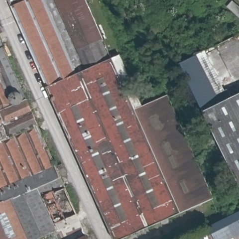
Sentinel-2 time series

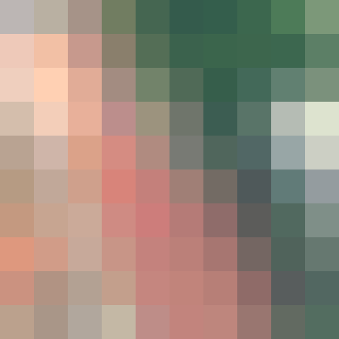
(a) FLAIR

Very high resolution RGB+NIR
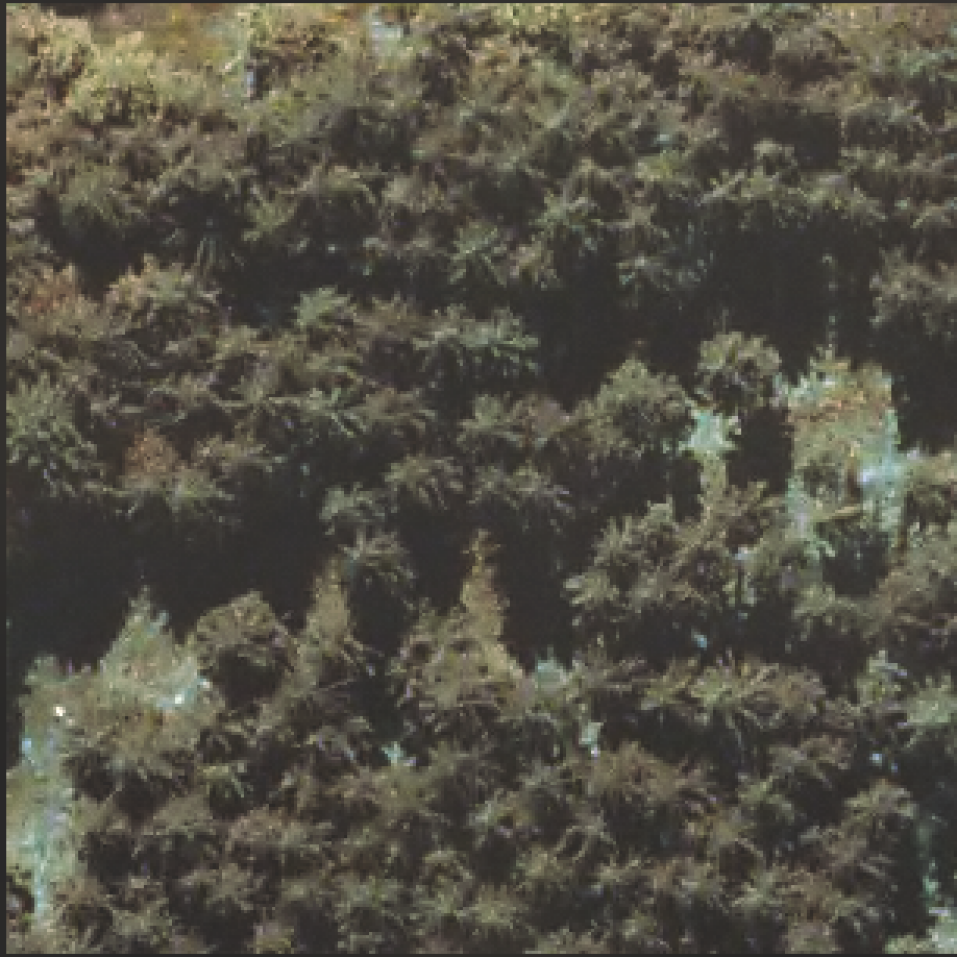
$\star$ Sentinel-2 time series
	black$\rightarrow$
$\star$ Sentinel-1 time series
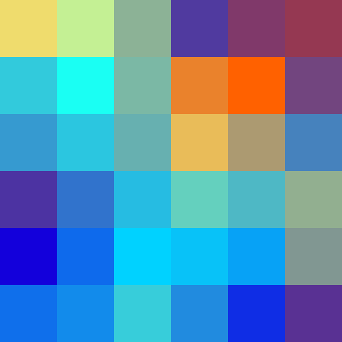
	black$\rightarrow$

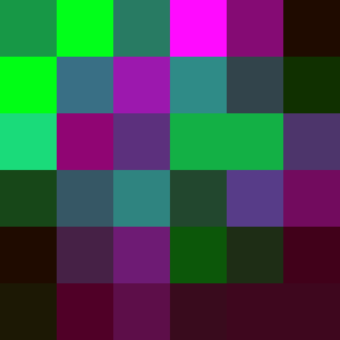
(b) TreeSatAI-TS

PASTIS: Sentinel-2 time series

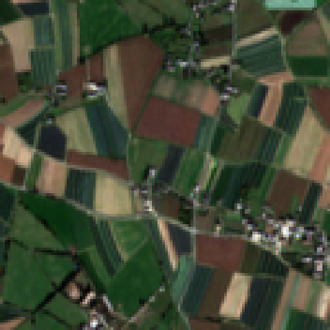
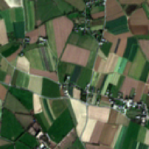
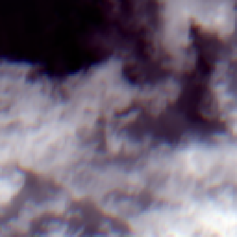
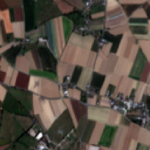
PASTIS-R: + Sentinel-1 time series

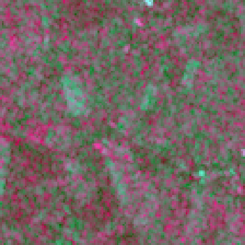
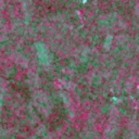
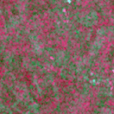
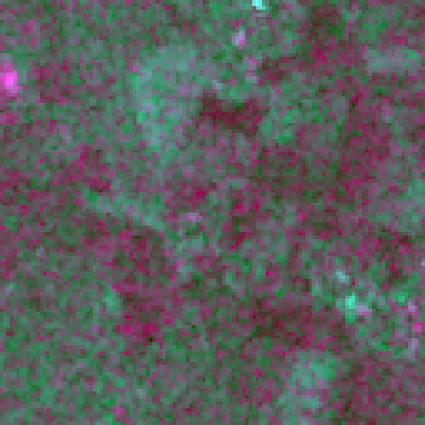
$\star$ Very high resolution RGB

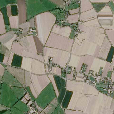
(c) PASTIS-HD

Figure 1: Datasets. We represent three tiles from our considered multilabel classification datasets: FLAIR (1(a)), TreeSatAI-TS (1(b)) and PASTIS-HD (1(c)). TreeSatAI-TS is a new dataset built by replacing the single-date Sentinel-1 and 2 images of TreeSatAI [35] by year-long time series. PASTIS-HD (1(c)) is a version of PASTIS-R [37] enriched with VHR satellite images. NIR stands for Near-InfraRed. $\star$ : modalities added in this work.

Generative methods reason at the level of individual token—a small portion of the input, typically a patch for images [64]. The objective is to reconstruct the masked tokens of an input image in pixel [65, 66, 67] or feature space [68]. This principle has been successfully adapted to EO analysis [69, 70, 71], and was further extended to handle multiple spatial scales [72], multimodality [4, 5], or hyperspectral observations [73, 74].

Several hybrid approaches combine the discriminative power of contrastive methods and the scalability of generative objectives for natural images [51, 75] and EO data [4]. Our proposed OmniSat also implements both mechanisms. A key difference is that the precise alignment between different sources of EO data allows us to contrastively match small patches of different modalities rather than entire images or time series.

Self-Supervised Multimodal Learning.

Multimodal computer vision has received a lot of interest [76], notably due to the success of cross-modal pre-training [32]. Recent models align the embeddings of heterogeneous modalities such as video and sound [33], depth and images [77], text and image [78, 79], or multiple combinations of these modalities [3, 2, 22, 23].

Multimodal learning also has a long history in EO [80, 81, 82] due to the large variety and complementarity of sensors [6, 7]. However, recent transformer-based architectures [83] for EO are often limited to one type of modality, be it a single image [70, 72] or time-series [84, 37]. For example, CROMA [4] and PRESTO [85] are specifically designed for paired optical and radar observations, but cannot handle very high resolution (VHR) data. USat [5] considers images with different resolutions, but only takes a single date within a time series. UT&T [48] can natively take single and multi-date observations of different modalities, but cannot be easily pre-trained in a self-supervised manner since it relies on convolutions and an ad-hoc late fusion scheme.

Multimodal EO Datasets.

As reported in Table 1, many multimodal EO datasets use Sentinel-1 [86] and 2 [19] data for applications ranging from land cover to forestry analysis and fire detection. We also note that most multimodal datasets only contain data of one type: mono-date image or time series. Several datasets (BigEarthNet [39], DFC20 [40], MDAS [41]) select a single date from time series. However, single Sentinel-1 and 2 acquisitions can be significantly affected by rain and cloud cover, respectively. Furthermore, capturing the temporal dynamics is crucial to characterize the phenology of vegetation [87],

FLAIR [48] is the first multimodal EO dataset to propose both very high spatial resolution ($\leq 2$m) and high temporal resolution ($>4$ images/year). Satlas [49] combines sentinel-2 time series and for 5% to tiles (continental US), very high definition NAIP images. The functional map of the World [88] integrates observations from various sensors, but most areas are only observed with one sensor. Two other datasets contain time series and single images from multiple sources, but were not available at the time of submission: IARPA-SMART [89] and DOFA [90].

To showcase how OmniSat can consume an arbitrary number of modalities with different spatial, spectral, and temporal resolutions, we selected two commonly used EO benchmarks, TreeSatAI [35] and PASTIS-R [37], whose focus on crop type mapping and forestry differs from the land cover analysis of FLAIR. We added new modalities to these datasets to reach three distinct data types: VHR aerial images, optical time series, and SAR time series. See Figure 1 for an illustration, and Section 4.1 for more details on how we extended these datasets.

Figure 2: OmniSat Architecture. We illustrate OmniSat for $M=3$ modalities, and a tile split into $P=4$ patches. The $M\times P$ input tokens $x^{\mathbf{M}}_{\mathbf{P}}$ are encoded by $M$ modality-specific encoders $\mathcal{E}^{\mathbf{M}}$, yielding the token representations $f^{\mathbf{M}}_{\mathbf{P}}$. The module $\mathcal{C}$ combines them into multimodal patch representations $f^{\star}_{\mathbf{P}}$. The token embeddings $f^{\mathbf{M}}_{\mathbf{P}}$ are supervised by a contrastive cross-modal objective. We also use a reconstruction objective: the masked multimodal representations $f^{\star}_{\mathbf{P}}$ are decoded by modality-specific networks $\mathcal{D}^{\mathbf{M}}$ to reconstruct their corresponding inputs in $x^{\mathbf{M}}_{\mathbf{P}}$.

3 Method

We consider a multimodal dataset $x$, defined as a collection of tiles divided into a set $\mathbf{P}$ of $P$ small spatial patches. We denote by $\mathbf{M}$ the set of $M$ available modalities. The patches are defined consistently across modalities: $x^{\mathbf{M}}_{p}=\{x^{m}_{p}\}_{m\in\mathbf{M}}$ corresponds to $M$ distinct views of the same patch $p$ with different sensors or modalities. Each modality $m$ has its unique input space $\Omega^{m}$ such that $x^{m}_{p}\in\Omega^{m}$. We define an input token as a pair $(m,p)$ for a given modality $m$ and a patch $p$, for a total of $M\times P$ tokens.

Our goal is to learn multimodal representations $f^{\star}_{p}$ that capture the content of each spatial patch $p$ captured by all modalities $\mathbf{M}$ in a self-supervised fashion. To achieve this, we employ a cross-modal contrastive objective (Section 3.1) and a multimodal masked encoding task (Section 3.2). We then give further details on the implementation of each module in Section 3.3. The overall architecture is represented in Figure 2.

3.1 Contrastive Objective

We associate each modality $m$ with a dedicated patch encoder $\mathcal{E}^{m}:\Omega^{m}\mapsto\mathbf{R}^{d}$ and denote by $f^{m}_{p}=\mathcal{E}^{m}(x^{m}_{p})$ the $d$-dimensional embedding of the input token $x^{m}_{p}$. We would like $f^{m}_{p}$ to capture robust and expressive features of $x^{m}_{p}$. To do so, we build a matching objective: patches should have consistent embeddings across modalities. Indeed, while each modality captures distinct characteristics of $p$, all encodings $f^{m}_{p}$ share the same latent variable: the semantic content of patch $p$.

In practice, we want $f^{m}_{p}$ close to $f^{n}_{p}$ for $n\neq m$, but far from $f^{n}_{q}$ for other patches $q\neq p$. We adapt the classic InfoNCE loss [91] to our setting with two main differences, illustrated in Figure 3: (i) each token $(m,p)$ has $M-1$ positive matches: the tokens corresponding to the same patch $p$ but viewed in another modality $n\neq m$; and (ii) as EO observations are generally spatially regular, nearby patches may be visually indistinguishable. Therefore, we exclude from the negative matches of $(m,p)$ all tokens in modality $m$ that are too close to $p$. To this end, we remove the set $T(m,p)$ of tokens with modality $m$ and whose patches are in the same tile as $p$. Our loss function $\mathcal{L}_{\text{contrast}}$ is defined as such:

$$\mathcal{L}_{\text{contrast}}=\frac{1}{MP}\sum_{(m,p)\in\mathbf{M}\times\mathbf{P}}\log\left(\frac{\sum_{n\neq m}\exp(\langle f^{m}_{p},f^{n}_{p}\rangle/\gamma)}{\sum_{(n,q)\in\mathbf{M}\times\mathbf{P}\setminus T(m,p)}\exp(\langle f^{m}_{p},f^{n}_{q}\rangle/\gamma)}\right)~{},$$ (1)

with $\gamma$ a temperature parameter, and $\langle\cdot,\cdot\rangle$ the scalar product in $\mathbb{R}^{d}$. This function, specifically designed for geospatial data, allows us to contrast individual patches across modalities, which is not typically feasible for natural images. However, as the contrastive objective aligns multimodal representations, the patch encoders $\mathcal{E}^{\mathbf{M}}$ may be encouraged to overlook the distinct attributes of their respective modality. Instead, they may focus only on features shared by all modalities, i.e. their common denominator. To ensure that encoders also capture modality-specific information, we incorporate a reconstruction objective, detailed in Section 3.2.

			$T_{1}$						$T_{2}$
			$m_{1}$		$m_{2}$		$m_{3}$		$m_{1}$		$m_{2}$		$m_{3}$
			$p_{1}$	$p_{2}$	$p_{1}$	$p_{2}$	$p_{1}$	$p_{2}$	$q_{1}$	$q_{2}$	$q_{1}$	$q_{2}$	$q_{1}$	$q_{2}$
$T_{1}$	$m_{1}$	$p_{1}$	o	o	+	-	+	-	-	-	-	-	-	-
		$p_{2}$	o	o	-	+	-	+	-	-	-	-	-	-
	$m_{2}$	$p_{1}$	+	-	o	o	+	-	-	-	-	-	-	-
		$p_{2}$	-	+	o	o	-	+	-	-	-	-	-	-
	$m_{3}$	$p_{1}$	+	-	+	-	o	o	-	-	-	-	-	-
		$p_{2}$	-	+	-	+	o	o	-	-	-	-	-	-
$T_{2}$	$m_{1}$	$q_{1}$	-	-	-	-	-	-	o	o	+	-	+	-
		$q_{2}$	-	-	-	-	-	-	o	o	-	+	-	+
	$m_{2}$	$q_{1}$	-	-	-	-	-	-	+	-	o	o	+	-
		$q_{2}$	-	-	-	-	-	-	-	+	o	o	-	+
	$m_{3}$	$q_{1}$	-	-	-	-	-	-	+	-	+	-	o	o
		$q_{2}$	-	-	-	-	-	-	-	+	-	+	o	o

Figure 3: Contrastive Loss. We represent the token matching matrix for two tiles $T_{1}$ and $T_{2}$ viewed across $3$ modalities $m_{1}$, $m_{2}$, and $m_{3}$. $T_{1}$ is composed of the patches $p_{1}$ and $p_{2}$, while $T_{2}$ comprises $q_{1}$ and $q_{2}$. In contrast to classic approaches which ignore the diagonal and assign each sample with a single positive match, our loss defines operates at the patch level, considers multiple positives per token, and excludes tokens in a block-diagonal fashion.

positive match negative match ignored

3.2 Multimodal Reconstruction Objective

This section introduces the modality combiner network $\mathcal{C}$ and its reconstruction objective. We mask a fraction of tokens $\mathbf{K}\subset\mathbf{M}\times\mathbf{P}$ and replace their embeddings with a learned vector $f^{\text{mask}}\in\mathbb{R}^{d}$. Note that the masking can differ across modalities, and some patches may be entirely masked. All tokens are then processed by the modality combining network $\mathcal{C}$, which outputs $P$ multimodal embeddings $f^{\star}_{\mathbf{P}}$:

$$f_{\mathbf{P}}^{\star}=\mathcal{C}\left(\{f^{m}_{p}\}_{(m,p)\not\in\mathbf{K}}\cup\{f^{\text{mask}}\}_{(m,p)\in\mathbf{K}}\right)~{}.$$ (2)

To encourage the patch embeddings $f^{\star}_{\mathbf{P}}$ to capture information from all modalities, we build a multimodal reconstruction objective. We equip each modality $m$ with a dedicated decoder $\mathcal{D}^{m}:\mathbb{R}^{d}\mapsto\Omega^{m}$ and write the reconstruction loss as:

$$\mathcal{L}_{\text{reconstruction}}=\frac{1}{|\mathbf{K}|}\sum_{(m,p)\in\mathbf{K}}\frac{1}{\text{dim}(\Omega^{m})}\left\|\mathcal{D}^{m}(f^{\star}_{p})-x^{m}_{p}\right\|^{2}~{},$$ (3)

where $\text{dim}(\Omega^{m})$ is the dimension of the input space $\Omega^{m}$. The total loss is the sum of $\mathcal{L}_{\text{reconstruction}}$ and $\mathcal{L}_{\text{contrast}}$.

3.3 Implementation

This section presents the tokenization process, the structure of the encoder and decoder for each modality, and the architecture of the modality combiner network. In particular, we highlight several design choices that leverage the specific properties of EO data [92].

Multimodal Tokenization.

All available modalities are spatially aligned through georeferencing. We split each tile along a regular spatial grid to produce a set of non-overlapping patches $\mathbf{P}$ consistent across all modalities, thus ensuring that $x^{\mathbf{M}}_{p}$ correspond to the same area for all modalities.

For TreeSat and FLAIR, we use a $10\times 10$m grid, meaning that the VHR input tokens are small image patches of size $50\times 50$ with $0.2$m per pixel. The patches of Sentinel observations with a resolution of $10$m are single-pixel temporal sequences of spectral measurements. For PASTIS-HD, we use a $40\times 40$m grid, meaning that the VHR patches are of size $40\times 40$ with $1.0$m per pixel. The patches of Sentinel observations [19] are $4\times 4$ image time series which we spatially flatten before encoding.

Time series from Sentinel satellites may experience registration errors spanning several meters, complicating their precise alignment with high-resolution imagery. However, using temporal sequences of satellite data mitigates these errors as aggregation over time tends to balance out misalignments.

Encoder-Decoder for Images.

Image tiles are split into small square patches: $\Omega^{\text{img}}=\mathbb{R}^{C\times I\times I}$ with $I$ the size of the patches and $C$ the number of channels. As shown in Figure 4(a), we encode these inputs with a sequence of convolutions and max-pool layers until the spatial dimension is fully collapsed. Decoding involves a symmetric sequence of convolutions and un-pooling layers. Contrary to existing masked auto-encoders, we pass the pooling indices from the encoder’s max-pooling to the decoder’s un-pooling in the manner of SegNet [93]. This dispenses the encoder from learning the intra-token spatial configuration and allows it to focus on the radiometric information, which may be more relevant depending on the application.

(a) Image Encoder and Decoder.

(b) Temporal Encoder and Decoder.

(c) Modality Combining Network.

Figure 4: Module’s Architectures. (4(a)) represents the encoder and decoder of image patches, and (4(b)) illustrates their architectures for temporal patches with a length of $L=4$ time stamps. The modality combining module $\mathcal{C}$ is depicted in (4(c)) with $P=2$ and $M=3$. Elements colored in orange are learned networks or parameters.

Encoder-Decoder for Time Series.

Each temporal patch is represented by $L$ sequential observations with $C$ channels: $\Omega^{\text{TS}}=\mathbb{R}^{C\times L}$, each associated with a time stamp. We encode the temporal patches using a Lightweight Temporal Attention Encoder (LTAE) model [94], an efficient network for geospatial time series processing. We decode each multimodal embedding $f^{\star}_{p}$ into temporal patches by repeating it $L$ times across the temporal dimension, adding a temporal encoding for each time step, and using an MLP to map the results to size $C$. See Figure 4(b) for an illustration.

Optical time series are notoriously affected by clouds [95]. This may affect the validity of the reconstruction task: the decoder cannot know which observations are cloudy, making the reconstruction objective unpredictable. To circumvent this issue, we use the temporal attention maps of the encoder’s LTAE to select dates to reconstruct: cloudless observations are more informative and should have a higher attention score [96]. We only consider in the reconstruction loss $\mathcal{L}_{\text{reconstruction}}$ the top $25\%$ dates in terms of the LTAE’s attention maps.

Modality Combining Network.

The modality combining network $\mathcal{C}$, represented in Figure 4(c), takes the $M\times P$ token embeddings ${f}^{\mathbf{M}}_{\mathbf{P}}$, some of whom can potentially be masked. We equip each token with a Euclidean relative positional encoding [97] calculated based on their patch’s position $\{r(p,q)\mid(p,q)\in\mathbf{P}^{2}\}$, and only defined for patches within the same tile. This way, each token can selectively consider its spatial surroundings. As most EO data are captured from above (satellite or aerial), their distribution is invariant by horizontal translation, making this choice of encoding preferable to an absolute position encoding.

The modality combining module $\mathcal{C}$ starts with a series of $B$ residual self-attention blocks connecting all tokens across modality and within the same tile. We then perform cross-attention between the resulting token embeddings $g^{\mathbf{M}}_{\mathbf{P}}\in\mathbb{R}^{d\times M\times P}$ and $P$ copies $f^{\text{comb}}_{\mathbf{P}}$ of a modality combining token $f^{\text{comb}}\in\mathbb{R}^{d}$ learned as a free parameter. Each copy of $f^{\text{comb}}_{p}$ is spatially located at the patch $p$ for the relative positional encoding $r$. The mechanism of $\mathcal{C}$ writes:

$$g^{\mathbf{M}}_{\mathbf{P}} =\text{self-attention}\left({f}^{\mathbf{M}}_{\mathbf{P}};r\right)~{},$$ (4)

$${f}^{\star}_{\mathbf{P}} =\text{cross-attention}\left(f^{\text{comb}}_{\mathbf{P}},g^{\mathbf{M}}_{\mathbf{P}};r\right)~{}.$$ (5)

Hyperparameters.

To show the versatility of OmniSat, we use the same configuration throughout all experiments. The embedding size is $d=256$, resulting in image encoders and decoders with $3.6$M and $1.8$M parameters, $403$K and $96$K for optical time series, and $402$K and $95$K for radar time series. The modality combiner module is composed of $B=6$ residual self-attention blocks and a single cross-attention block, for a total of $3.6$M parameters. We train our model with the ADAM optimizer [98], with a learning rate of $10^{-4}$ for pretraining and $2\times 10^{-5}$ for fine-tuning, and a ReduceLROnPlateau scheduler [99] with a patience of $10$ epochs and a decay rate of $0.1$. When re-implementing competing methods, we use the hyperparameters of their open-source repository.

4 Experiments

In this section, we evaluate OmniSat’s performance across three multimodal datasets, including two new datasets introduced in this work and presented in Section 4.1. We outline our experimental protocol and our adaptation of competing methods in Section 4.2. We then present in Section 4.3 our quantitative results and analysis, and qualitative results in Figure 5. Lastly, we conduct an ablation study to in Section 4.4.

4.1 Datasets

We evaluate OmniSat on three multimodal datasets: FLAIR [48], and the augmented TreeSatAI-TS [35] and PASTIS-HD [36, 37]. See Figure 1 for an illustration of these two datasets.

TreeSatAI-TS:

TreeSatAI [35] is a multimodal dataset for tree species identification, containing $50,381$ tiles of $60\times 60$m with multi-label annotations for $20$ classes and all taken in Germany. Each tile is associated with a very high resolution RGB and near-infrared (NIR) image ($0.2$m pixel resolution), a single Sentinel-2 multi-spectral image (10m per pixel resolution, 10 bands), and a single Sentinel-1 radar image (10m per pixel resolution, 3 bands: two polarization channels and their ratio).

Motivated by the fact that fine-grained vegetation discrimination relies heavily on temporal dynamics information [87], we introduce TreeSatAI-TS. This extended version uses open-source data to add Sentinel-1 and Sentinel-2 time series to each tile, spanning the closest available year to the VHR observation for Sentinel-2. Note that due to the weather patterns and position of the area of interest with respect to Sentinel-2’s orbit, the optical time series is particularly irregular and occluded, with up to $50$% of acquisitions being non-exploitable. Despite this challenge, we included the raw observations without pre-processing, whereas TreeSatAI’s single-date images have been manually selected.

PASTIS-HD:

The PASTIS dataset [36], is designed for semantic and panoptic segmentation of agricultural parcels using Sentinel-2 time series and covers $18$ crop types across $2433$ image time series with dimensions of $1280\times 1280$m. Each series contains between $38$ and $61$ observations with $10$ spectral bands. PASTIS-R [37] adds the corresponding Sentinel-1 radar time series. We only used the ascendent time series of Sentinel-1 for our training and evaluation, for a total of 169,587 radar images with three bands.

To enhance the spatial resolution and utility of PASTIS, we introduce PASTIS-HD, which integrates contemporaneous VHR satellite images (SPOT 6-7 [100]). We apply orthorectification and pansharpening, resample the resulting images to a $1$m resolution, and finally convert them to 8 bits.

We follow the protocol of Irvin et al. [5] to use the dense annotations for a multi-label classification task: each patch is associated with the labels of all its pixels. This conversion allows us to evaluate all methods in the same setting and configuration as TreeSatAI.

FLAIR.

The FLAIR dataset [48] combines VHR aerial images with time series data. It comprises $77,762$ aerial tiles ($512\times 512$ pixels, $0.2$m resolution) with five channels (RGB, near-infrared, and a normalized digital surface model) taken in France, alongside corresponding Sentinel-2 time series ($10$m resolution, $10$ spectral bands, $20$ to $114$ observations per year). We apply the same processing as PASTIS to use the dense annotation for a multi-label classification task.

	Inputs		Ground truth	OmniSat	UT&T [48]	Scale-MAE [72]
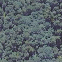
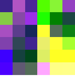
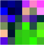
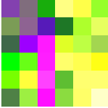
TreeSatAI-TS			- Picea - Betula - Alnus - Quercus	- Picea - Betula - Alnus - ✗	- Picea - Betula - Alnus - ✗ - Pinus	- Picea - ✗ - ✗ - ✗
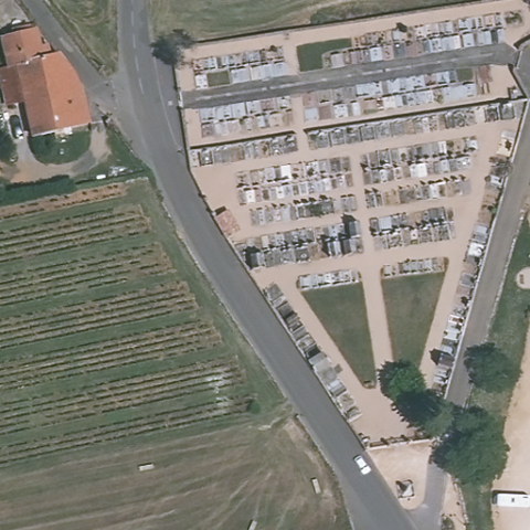
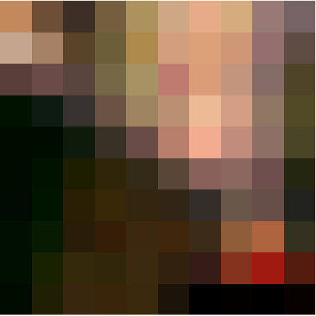
FLAIR			- building - pervious surf. - impervious surf. - deciduous - brushwood - herbaceous - agricultural - vineyard	- building - pervious surf. - impervious surf. - deciduous - brushwood - herbaceous - agricultural - vineyard	- building - pervious surf. - impervious surf. - deciduous - brushwood - herbaceous - agricultural - ✗	- building - pervious surf. - impervious surf. - deciduous - brushwood - herbaceous - ✗ - ✗
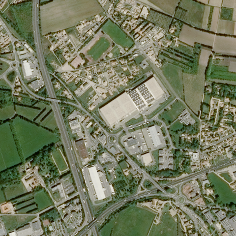
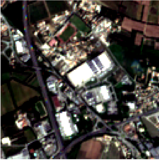
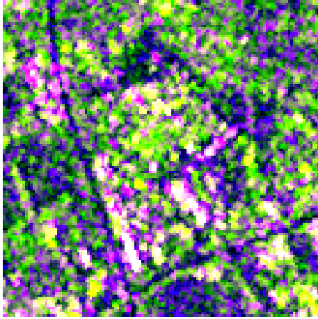
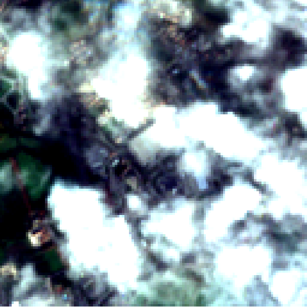
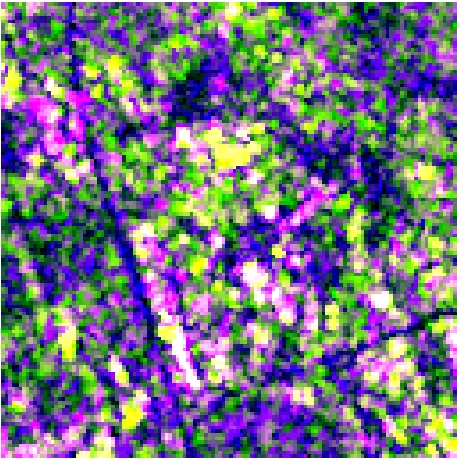
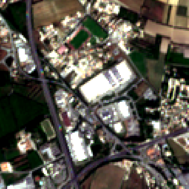
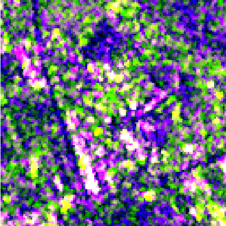
PASTIS-HD			- Meadow - Soft winter wheat - Corn - Winter rapeseed - Beet	- Meadow - Soft winter wheat - Corn - Winter rapeseed - Beet	- Meadow - ✗ - ✗ - ✗ - ✗ - Potatoes	- Meadow - ✗ - ✗ - ✗ - ✗ - Sunflower - Grapevine

Figure 5: Qualitative Results. We report predictions of OmniSat and two competing models on tiles from our datasets. OmniSat can detect classes with recognizable temporal dynamics such as agricultural lands or mixed forest areas with both coniferous  and deciduous trees . Other methods, and in particular ScaleMAE, struggle to detect these classes.

4.2 Experimental Setting

This section details our experimental protocol and our adaption of competing algorithms.

Evaluation Protocol.

All experiments follow a similar setting:

• Pre-training (optional). Methods that support self-supervised pre-training (OmniSat, SatMAE [70], ScaleMAE [72], CROMA [4]) are pre-trained for up to $250$ epochs on the entire training set without access to labels.

• Fine-Tuning. We propose two settings for fine-tuning:

  • Fully Supervised Fine-Tuning. We train the resulting models using all the labels in the training set.

  • Semi-Supervised Fine-Tuning. We use a portion of $10$% or $20\%$ of the training set, stratified by the distribution of classes, to fine-tune the models. For models without pre-training, this corresponds to supervision in the low-data regime.

• Monomodal and Multimodal Evaluation. We evaluate all methods using each available modality independently and combining all supported modalities.

Table 2: Performance on TreeSatAI-TS. We report the weighted F1 for multi-label tree species classification on TreeSatAI (TSAI) and our extended TreeSatAI-TS (TSAI-TS) dataset when fine-tuning with $10$% and $100$% of training labels. The first line line of the table is the modality used for evaluation. We distinguish methods that are best for one modality within a dataset, best in a dataset across all modalities, and the best overall performance. ^⋆: late feature fusion with a ResNet. $\scalerel*{{\dagger}}{X}$: model evaluated on this dataset for the first time.

Model	pre-	All		Sentinel-1		Sentinel-2		VHR Image
	training	10%	100%	10%	100%	10%	100%	10%	100%
Evaluated on TreeSatAI: single date for Sentinel-1 and Sentinel-2
MLP[35]	ImageNet	42.6⋆	71.5⋆	3.4	10.1	22.1	52.0	-	-
ResNet [35]	ImageNet	-	-	-	-	-	-	58.8	70.1
LightGBM [35]	ImageNet	-	54.3⋆	-	11.9	-	48.2	-	44.0
$\scalerel*{{\dagger}}{X}$ PSE [101]	None	47.2⋆	68.1⋆	11.5	14.6	48.5	58.3	-	-
$\scalerel*{{\dagger}}{X}$ ViT [64]	None	42.7⋆	57.1⋆	8.7	17.5	39.8	57.3	36.7	51.7
PRESTO [85]	PRESTO	-	-	-	19.8	-	46.3	-	-
MOSAIKS [102, 103]	TSAI	-	-	-	-	-	56.0	-	-
$\scalerel*{{\dagger}}{X}$ CROMA [4]	TSAI	49.6⋆	61.0⋆	10.1	12.7	47.8	55.7	-	-
$\scalerel*{{\dagger}}{X}$ SatMAE [70]	TSAI	46.1⋆	61.5⋆	-	-	40.3	49.7	44.1	61.4
$\scalerel*{{\dagger}}{X}$ ScaleMAE [72]	TSAI	47.6⋆	62.5⋆	-	-	46.7	55.2	46.9	63.6
OmniSAT (ours)	TSAI	56.2⋆	70.4⋆	5.3	6.4	48.4	57.1	52.8	68.9
Evaluated on TreeSatAI-TS: Sentinel-1 and Sentinel-2 time series spanning one year
$\scalerel*{{\dagger}}{X}$ UT&T [48]	ImageNet	43.8⋆	56.7⋆	42.3	55.2	41.5	57.0	44.3	55.9
$\scalerel*{{\dagger}}{X}$ Scale-MAE [72]	TSAI-TS	44.1⋆	60.4⋆	-	-	11.0	31.5	46.9	63.6
$\scalerel*{{\dagger}}{X}$ PSE+LTAE [101]	None	59.4⋆	71.2⋆	42.6	52.4	44.0	57.2	-	-
OmniSAT (ours)	None	52.2⋆	73.3⋆	31.6	55.9	33.9	49.7	51.4	71.0
OmniSAT (ours)	TSAI-TS	61.1	74.2	48.2	56.7	51.4	62.9	58.3	70.5

Adapting Competing Approaches.

We report the performance of several methods taken from the literature on our considered datasets: LightGBM [35], PRESTO [85], and MOSAIKS [103]. However, few existing methods can operate on single- and multi-date data at the same time. To ensure a fair evaluation of competing approaches, we modify various state-of-the-art models to handle a broader combination of modalities. We performed multiple tests for each approach and kept the configurations leading to their highest performance.

• Multimodality. We train methods that are not natively multimodal (PSE [101], ViT [64], SatMAE, ScaleMAE) using a late-fusion scheme [104] by concatenating the embeddings learned in each modality, as suggested by Ahlswede et al. [35]. For UT&T [48], initially designed for VHR images and Sentinel-2 time series, we add a branch for Sentinel-1 integration, which is identical to the Sentinel-2 branch except for the first layer.

• Handling Temporal Data. To evaluate image models (SatMAE, ScaleMAE, CROMA) on time series, we convert image sequences to single images by concatenating for each pixel and channel channel-wise the median observation for the four seasons: spring, summer, fall, and winter [105].

• Handling VHR Data. To evaluate methods designed for low-resolution images (PSE, LTAE [94]) in a multimodal setting that includes VHR images, we concatenate the representations obtained with a ResNet network to their final embedding.

• Scaling Models. Our considered datasets are smaller than the ones used to train large ViT-based models, making them prone to overfitting. We address this issue by selecting a ViT-Small [64] backbone instead of a ViT-Large for SatMAE, ScaleMAE and CROMA.

• Multi-Class Prediction. To evaluate ViT-based models on classification experiments, we insert a linear layer that maps the embedding of the class token $\langle\texttt{CLS}\rangle$ to a vector of class scores. For the UT&T model, we compute a spatial average of the last feature map, followed by a similar linear projection.

Table 3: Performance on PASTIS-HD. We report the macro-averaged F1-score for crop-type multi-class classification on the PASTIS-HD dataset. We distinguish methods that are best for one modality, best in a dataset across all modalities. ^⋆: late feature fusion with a ResNet. $\scalerel*{{\dagger}}{X}$: model evaluated on this dataset for the first time.

Model	pre-	All		Sentinel-1		Sentinel-2		VHR image
	trained	20%	100%	20%	100%	20%	100%	20%	100%
$\scalerel*{{\dagger}}{X}$ ResNet50 [106]	ImageNet	-	-	-	-	-	-	57.6	59.3
$\scalerel*{{\dagger}}{X}$ Scale-MAE [72]	PASTIS-HD	42.0⋆	42.2⋆	-	-	41.2	46.1	48.8	51.9
$\scalerel*{{\dagger}}{X}$ UTAE [36, 37]	No	36.8⋆	46.9⋆	20.1	40.7	32.7	37.6	-	-
$\scalerel*{{\dagger}}{X}$ UT&T [48]	ImageNet	54.2⋆	53.5⋆	58.8	62.8	54.9	61.3	51.1	49.8
$\scalerel*{{\dagger}}{X}$ CROMA [4]	PASTIS-HD	57.5⋆	60.1⋆	55.3	56.1	53.0	56.7	-	-
OmniSAT (ours)	No	42.0⋆	59.1⋆	58.2	60.2	51.7	60.1	47.3	52.8
OmniSAT (ours)	PASTIS-HD	62.6⋆	69.9⋆	60.8	69.0	61.8	70.8	54.6	59.3

Table 4: Performance on FLAIR. We report the macro-averaged F1-score for land cover multi-class classification on the FLAIR dataset. We distinguish methods that are best for one modality and best in a dataset. $\scalerel*{{\dagger}}{X}$: model evaluated on this dataset for the first time.

Model	pre-	All		Sentinel-2		VHR Image
	trained	10%	100%	10%	100%	10%	100%
$\scalerel*{{\dagger}}{X}$ UT&T [48]	ImageNet	44.2	48.8	57.4	62.0	58.9	65.5
$\scalerel*{{\dagger}}{X}$ ScaleMAE[72]	FLAIR	63.1	70.0	52.5	61.0	61.2	67.3
OmniSAT (ours)	No	62.5	70.0	56.1	65.4	64.7	71.5
OmniSAT (ours)	FLAIR	60.6	73.4	56.8	65.4	65.2	71.6

4.3 Numerical Experiments and Analysis

In this section, we report our model’s performance and efficiency compared to other approaches across the considered datasets and propose our analysis.

TreeSatAI-TS.

Table 2 presents the performance of different models on TreeSatAI and TreeSatAI-TS. We report several key observations:

• Benefit of Time Series. For the original TreeSatAI dataset with single-date Sentinel-1/2 observations, none of the pre-training schemes significantly improve performance beyond simple baselines such as ResNet, PSE, or MLP, even in a semi-supervised setting. In particular, single-date S1 observations yield low performance for all methods (below $20$ F1-score), emphasizing the need to use the entire time series.

  OmniSat exhibits significantly improved results on TreeSatAI-TS, with or without pretraining. In contrast, Scale-MAE struggles to extract meaningful dynamic features from the highly occluded time series, and CROMA would not converge. These models perform better with the manually chosen single-date images of TreeSatAI than with temporally aggregated temporal observations, whereas OmniSat can leverage dynamic features.

• Benefits of Multimodality. When using all modalities, OmniSat outperforms all competing methods by a margin of $3$% F1-score. The multimodal performance of OmniSat and CROMA, which learn to combine data sources, is strictly superior to the F1-score of their best modality by $3.7$% and $5.3$% points, respectively. Conversely, the performance of methods that rely on late-fusion (SatMAE, ScaleMAE, ViT) is comparable to their best modality. This demonstrates the value of learning to combine information from different sources end-to-end.

• Benefits of Cross-Modal Pre-Training. With access to all modalities, our self-supervised pre-training improves by $0.9$% point the F1-score of the model fine-tuned on $100$% of labels, compared to not pre-training, and $8.9$% when using only $10$% of labels. This shows that our pre-training leads to more expressive multimodal features. Interestingly, when performing inference with Sentinel-2 time series alone, the performance increase linked to the pre-training becomes $13.2$% with $100$% labels and $17.5$% with $10$%. This illustrates that our pre-training scheme also improves the features learned by each encoder despite only relying on spatial matching.

Figure 6: Efficiency. We report the best performance of different models between TreeSatAI and TreeSatAI-TS, with pre-training and fine-tuning using $100$% of labels. The area of the markers is proportional to the training time, broken down in pre-training and fine-tuning when applicable.

Experiments on PASTIS-HD.

The analysis of the performance of various models on PASTIS-HD is reported in Table 3, and is consistent with the ones of TreeSatAI-TS. First, by learning to combine all modalities despite their different resolutions, OmniSat achieves state-of-the-art results on this benchmark. Second, our cross-modal pertaining significantly improves OmniSat’s performance in the multimodal (+10.8 pF1-score with 100% of training label) and all single-modality settings ($8.8$ points for Sentinel-1, $10.7$ for Sentinel-2, and $6.5$ for the VHR images).

Experiments on FLAIR.

We report in Table 4 the results on the bimodal FLAIR dataset for multilabel classification. OmniSat outperforms the much larger ScaleMAE [72] and UT&T [48] models with $100$% of labels and both modalities by $3.4$%. Our pre-training scheme had a smaller impact than for the TreeSatAI-TS experiment, which may be attributed to the fact that only two modalities are available, which decreases the supervisory power of our cross-modal contrastive objective and our multimodal reconstruction loss. This highlights a limitation of OmniSat: the model needs to be pretrained on a modality-rich dataset to achieve its best performance. We also note the poor performance of UT&T, which we attribute to its semantic segmentation-driven design.

Efficiency Evaluation.

We plot in Figure 6 the best performance between TreeSatAI and TreeSatAI-TS for different models according to their size and training time. OmniSat is more compact, faster to train, and performs better than all evaluated models. The highly-specialized combination of PSE, LTAE, and ResNet is a strong contender, outperforming significantly more complex models with generic encoding-decoding schemes.

4.4 Ablation Study

In this section, we report the results of several experiments evaluating the impact and validity of our main design choices, see Table 5.

a) Encoder/Decoder Architecture.

We propose several improvements to the standard image encoder-decoder scheme used in computer vision to accommodate the specificities of EO data. In particular, passing the max-pool indices from the image patch encoder to its decoder allows the learned representation to focus on characterizing the spectral signature instead of fine-grained spatial information, and leads to a performance increase of $0.7$% in the full supervision setting.

As clouds frequently obstruct optical time series, we use an unsupervised date-filtering scheme to reconstruct only meaningful acquisitions. This approach leads to a significant improvement of $3.6$%, showcasing the benefit of developing modality-aware approaches for EO.

b) Role of Loss Functions.

When training without contrastive loss, we observe a small decrease in performance of $0.8$% in the fully supervised regime and a more pronounced drop of $5.5$% in the semi-supervised regime. This demonstrates how harmonizing the encoding across encoders facilitates their subsequent fusion. Interestingly, when implementing a naive contrastive loss that considers negative examples within the same tile and modality, the decrease is greater than simply removing this loss ($2$% in full supervision). This strategy may introduce indistinguishable negative examples and perturb the learning process.

We also remove the reconstruction loss, meaning that only the encoders are learned contrastively during pre-training. This results in a drop of $2$% F1-score point, illustrating the importance of pre-training the transformer $\mathcal{C}$ alongside its encoders.

Limitations.

All datasets used in our experiments are based in Europe, primarily due to the availability of open-access annotations. This regional focus prevents us from evaluating our model’s performance in tropical and developing countries, which present unique challenges in terms of label provision, heterogeneity, and complex classes.

A limitation of our pre-training scheme is its dependence on a sufficient number of aligned modalities, as illustrated by its moderate impact on the bimodal FLAIR dataset.

Table 5: Ablation Study. We present the impact of several design choices on the TreeSatAI-TS dataset, measured in terms of macro-averaged F1-score.

Experiment	10%	100%	Experiment	10%	100%
OmniSat	61.1	74.2	b) no contrastive loss	55.6	73.4
a) no index bypass	57.5	73.5	b) naive contrastive loss	57.8	72.2
a) no date filtering	58.2	71.6	b) no reconstruction loss	59.0	72.2

5 Conclusion

We introduced OmniSat, a new architecture for the self-supervised modality fusion of Earth Observation (EO) data from various sources. To facilitate its evaluation, we augmented two existing benchmarks to form the first open-access datasets with three distinct modalities of different natures and resolutions. We experimentally showed that leveraging diverse modalities with a flexible model improves the model’s performance in both fully and semi-supervised settings. Moreover, our training scheme can exploit the spatial alignment of multiple modalities to improve our model’s monomodal performance. Finally, we proposed several improvements to leverage the unique structure of EO data in the architecture of our model, such as automatic date filtering for reconstructing time series and index bypass in image patch decoders. We hope that our promising results and new datasets will encourage the computer vision community to consider EO data as a playing field for evaluating and developing novel self-supervised multimodal algorithms.

Acknowledgements.

This work was supported by ANR project READY3D ANR-19-CE23-0007, and was granted access to the HPC resources of IDRIS under the allocation AD011014719 made by GENCI. We thank Anatol Garioud and Sébastien Giordano for their help on the creation of TreeSatAI-TS and PASTIS-HD datasets. The SPOT images are opendata thanks to the Dataterra Dinamis initiative in the case of the ”Couverture France DINAMIS” program. We thank Jordi Inglada for inspiring discussions and valuable feedback.

Appendix

In this appendix, we present an extended ablation study in Section 1, detailed classwise performance in Section 2, and analysis of failure cases on challenging examples in Figure 2.

1 Supplementary Ablations

We propose two supplementary ablation cases for a more in-depth analysis and comprehensive assessment of OmniSat:

Relative vs. Absolute Positional Encoding.

We evaluate the impact of replacing the relative positional encoding of tokens, based on the patch position, with an absolute position encoding, based on the position of the patches in their tile—similar to what is classically done for image processing.

With an absolute positional encoding, OmniSat reaches an F1-score of $58.4$ and $73.0$ when fine-tuned with $10$% and $100$% of the training set of TreeSatAI-TS, respectively. This is $2.7$ and $1.2$% below a model trained with relative positional encodings. We conclude that relative positional encodings are better suited for analyzing EO images. While the upper patches of natural images are bound to correspond to the sky, and the lower patches contain ground, no such analogy can be made for EO data, whose distribution is equivariant through small horizontal translation.

Impact of Pretraining on Monomodal Performance.

We aim to determine how our multimodal pretraining scheme improves the monomodal performance (e.g., +13.2% for Sentinel-2 in full supervision). We consider two mechanisms that may lead to more discriminative features: (i) multimodality allows us to train the modality combiner network $\mathcal{C}$ with more data, or (ii) our cross-modal and token-wise alignment-based losses provide a strong supervisory signal. We propose an experiment to verify which mechanism is the leading reason of our scheme’s strong performance.

We pre-train OmniSat on TreeSatAI-TS in mono- and multimodal settings with a constant amount of tokens. More precisely, we pre-train OmniSat using all input tokens from the S2 modality only, and using all $3$ modalities but only $33\%$ of patches. This means that each experiment considering the same number $P$ of input tokens. We then train a single linear layer to map these representations to class scores (linear probing) using $10$ and $100$% of the annotated S2 data. Finally, we evaluate the quality of these linear mappings on the test set using only the S2 modality.

The model trained with a multimodal pretext task reaches a F1-score of $44.7$ for $10$% and $46.3$ for $100$% of the training data. The model trained only with S2 performs significantly worse: $26.9$ for $10$% and $29.8$ for $100$% of data. This result suggests that the key to the efficacy of our pretraining scheme is the supervisory signal of per-patch contrastive and reconstruction objectives, rather than just increasing the number of tokens viewed by the transformer backbone.

2 Supplementary Results

We report the performance of different approaches for each class for the two datasets graphically in Figure 1 and as a table in Table 1.

Figure 1: Class-Wise Performance. We plot the performance of different models for each class, sorted by decreasing frequency. OmniSat improves the performance across the board, and for rare classes in particular.

TreeSatAI-TS

Method	Macro F1	​​​​Abies ​​​​	​​​​Acer ​​​​	​​​​Alnus ​​​​	​​​​Betula ​​​​	​​​​Cleared	​​​​Fagus ​​​​	​​​​Fraxinus ​​​​	​​​​Larix ​​​​	​​​​Picea ​​​​	​​​​Pinus ​​​​	​​​​Populus ​​​​	​​​​Prunus ​​​​	​​​​Pseudotsuga ​​​​	​​​​Quercus ​​​​	​​​​Tilia ​​​​
Proportion in %		2.5	6.5	6.5	7.1	11.2	22.6	5.7	9.7	21.8	23.0	1.8	0.8	8.9	22.8	0.5
UT&T	48.8	52.8	43.4	49.8	36.8	53.7	60.7	45.9	43.7	63.6	72.1	44.8	32.4	45.4	62.5	25.0
Scale-MAE	47.3	53.2	32.4	42.7	38.5	64.4	63.8	38.3	51.7	71.5	78.2	25.4	11.8	55.1	64.0	18.2
OmniSat	73.4	74.1	58.9	62.5	56.5	74.9	72.9	60.0	69.5	77.6	85.4	64.6	46.2	68.5	76.1	43.4

FLAIR

Method	Macro F1	​​​​building	​​​​perv. surface	​​​​imperv. surface	​​​​bare soil	​​​​water	​​​​coniferous	​​​​deciduous	​​​​brushwood	​​​​vineyard	​​​​herbaceous	​​​​agri. land	​​​​plowed land	​​​​other
Proportion in %		27.6	45.0	37.7	8.0	12.5	36.0	84.2	49.6	6.5	74.1	39.4	7.1	11.0
UT&T	57.3	52.4	63.3	60.4	32.7	46.9	64.4	91.2	66.3	57.1	84.7	71.7	27.1	26.2
Scale-MAE	70.0	90.1	72.0	87.1	47.1	81.3	65.1	95.2	72.3	53.7	88.8	70.2	39.7	45.7
OmniSat	75.8	91.8	73.2	88.2	54.4	81.3	70.6	95.2	73.4	72.1	87.5	71.1	36.0	48.5

PASTIS-HD

Method	Macro F1	​​​​Meadow	​​​​Soft winter wheat	​​​​Corn	​​​​Winter barley	​​​​Winter rapeseed	​​​​Spring barley	​​​​Sunflower	​​​​Grapevine	​​​​Beet	​​​​Winter triticale	​​​​Winter durum wheat	​​​​Fruits, vegetables, flowers	​​​​Potatoes	​​​​Leguminous fodder	​​​​Soybeans	​​​​Orchard	​​​​Mixed cereal	​​​​Sorghum
Proportion in %		94.4	63.7	61.9	46.4	29.0	19.4	17.3	20.0	12.3	19.8	15.1	22.6	12.7	42.7	14.9	17.7	19.6	15.3
UT&T	53.5	97.1	78.3	77.5	63.1	57.5	25.4	49.2	54.9	69.9	50.7	50.5	50.6	22.0	60.0	59.0	46.3	36.9	13.8
CROMA	60.1	97.1	87.1	88.9	64.2	86.5	41.1	64.5	74.2	76.5	51.2	74.3	61.3	26.1	53.3	59.1	45.9	22.4	9.1
Scale-MAE	42.2	97.1	84.2	83.3	56.4	53.6	15.1	24.1	54.9	39.1	27.5	43.9	41.5	12.3	48.1	34.2	30.4	12.5	2.6
OmniSat	69.9	97.2	90.1	92.2	82.6	89.0	64.7	75.0	82.7	88.1	48.5	81.3	56.7	52.6	56.9	85.7	48.4	34.8	31.7

Table 1: Class-Wise Performance. We report the F1-score for each class for TreeSatAI-TS, FLAIR, and PASTIS-HD for multilabel classification. We also report the unweighted class-averaged F1-score (Macro-F1). We can observe that OmniSat outperforms UT&T [48] and Scale-MAE [72] on nearly all classes for both datasets. In particular, we observe the most significant gains for classes with discriminative temporal dynamics, such as broadleaf tree species and the vineyards class.

Failure Case.

We report in Figure 2 hard examples from our three datasets and compare the prediction of OmniSat and other models. For the TreeSatAI-TS example, the Sentinel-2 optical time-series is highly occluded: over 80% of acquisitions are covered by clouds. Furthermore, the forest tile contains a large variety of tree species organized in densely connected canopy, making its classification particularly hard. Indeed, the texture of the images in closed forests does not bring additional discriminative information.

The example from FLAIR is a scrap yard, which is almost entirely covered by broken vehicles. Since FLAIR’s annotations focus on the ground rather than transient or stationary objects, identifying the actual land cover in such scenarios is very challenging.

The image taken from PASTIS contains a mix of several different crop types, including the class mixed cereal which can already correspond to a parcel with various cereal types. This leads to a hard classification problem for all methods.

	Inputs		Ground truth	OmniSat	UT&T [48]	Scale-MAE [72]
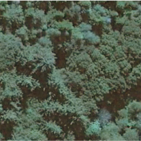
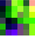
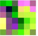
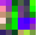
TreeSatAI-TS			- Quercus - Acer - Alnus - Larix	- Quercus - ✗ - ✗ - ✗ - Abies	- ✗ - ✗ - ✗ - ✗ - Abies - Betula	- ✗ - ✗ - ✗ - ✗ - Picea
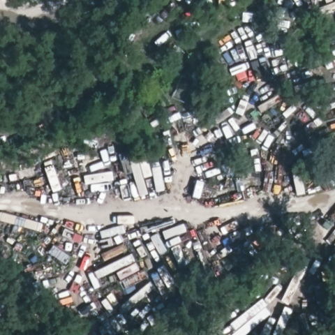
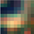
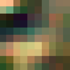
FLAIR			- decideous - herbaceous - water - pervious surf. - bare soil	- decideous - herbaceous - water - ✗ - ✗ - building - impervious surf. - brushwood	- decideous - herbaceous - ✗ - pervious surf. - ✗ - building - impervious surf. - brushwood - coniferous	- decideous - herbaceous - ✗ - pervious surf. - ✗ - building - impervious surf. - brushwood - coniferous - other
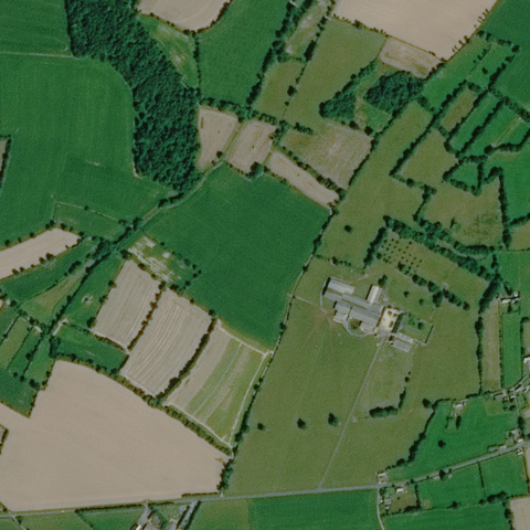
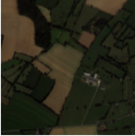
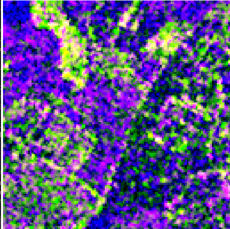
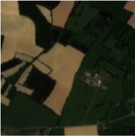
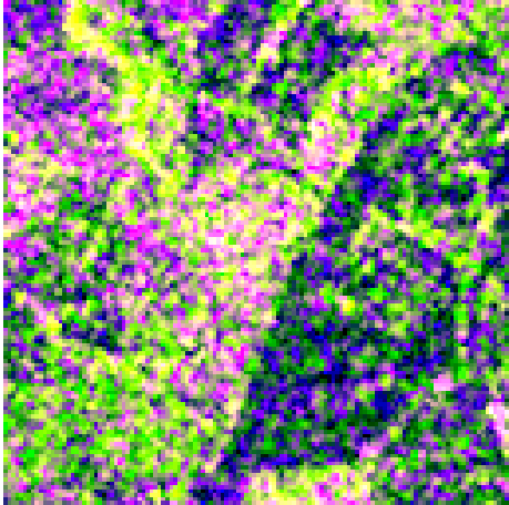
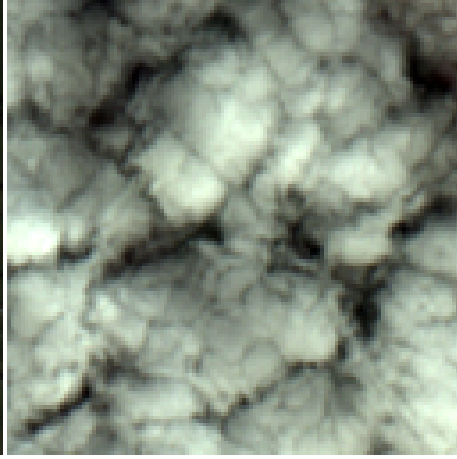
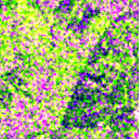
PASTIS-HD			- Meadow - Winter wheat - Corn - Potatoes - Mixed cereal	- Meadow - Winter wheat - Corn - Potatoes - ✗ - Winter barley - Winter rapeseed - Legum. fodder	- Meadow - ✗ - ✗ - ✗ - ✗ - Spring barley - Orchard - Legum. fodder - Durum wheat - Fruits, veg., flow.	- Meadow - Winter wheat - Corn - ✗ - ✗ - Winter barley - Winter rapeseed - Winter triticale

Figure 2: Failure Cases. We provide hard instances for the TreeSatAI-TS, FLAIR, and PASTIS-HD datasets, and report the multiclass prediction for OmniSat as well as two competing methods.

References

- Zong et al. [2023] Yongshuo Zong, Oisin Mac Aodha, and Timothy Hospedales. Self-supervised multimodal learning: A survey. arXiv preprint arXiv:2304.01008, 2023.
- Girdhar et al. [2023] Rohit Girdhar, Alaaeldin El-Nouby, Zhuang Liu, Mannat Singh, Kalyan Vasudev Alwala, Armand Joulin, and Ishan Misra. Imagebind: One embedding space to bind them all. In CVPR, 2023.
- Shukor et al. [2023] Mustafa Shukor, Corentin Dancette, Alexandre Rame, and Matthieu Cord. UnIVAL: Unified model for image, video, audio and language tasks. TMLR, 2023.
- Fuller et al. [2023] Anthony Fuller, Koreen Millard, and James R Green. CROMA: Remote sensing representations with contrastive radar-optical masked autoencoders. In NeurIPS, 2023.
- Irvin et al. [2023] Jeremy Irvin, Lucas Tao, Joanne Zhou, Yuntao Ma, Langston Nashold, Benjamin Liu, and Andrew Y Ng. USat: A unified self-supervised encoder for multi-sensor satellite imagery. arXiv preprint arXiv:2312.02199, 2023.
- Ghamisi et al. [2019] Pedram Ghamisi, Behnood Rasti, Naoto Yokoya, Qunming Wang, Bernhard Hofle, Lorenzo Bruzzone, Francesca Bovolo, Mingmin Chi, Katharina Anders, Richard Gloaguen, et al. Multisource and multitemporal data fusion in remote sensing: A comprehensive review of the state of the art. IEEE Geoscience and Remote Sensing Magazine, 2019.
- Schmitt and Zhu [2016] Michael Schmitt and Xiao Xiang Zhu. Data fusion and remote sensing: An ever-growing relationship. IEEE Geoscience and Remote Sensing Magazine, 2016.
- Coppin et al. [2002] Pol Coppin, Eric Lambin, Inge Jonckheere, and Bart Muys. Digital change detection methods in natural ecosystem monitoring: A review. Analysis of multi-temporal remote sensing images, 2002.
- Secades et al. [2014] Cristina Secades, Brian O’Connor, Claire Brown, Matt Walpole, et al. Earth observation for biodiversity monitoring: A review of current approaches and future opportunities for tracking progress towards the aichi biodiversity targets. CBD technical series, 2014.
- Skidmore et al. [2021] Andrew K Skidmore, Nicholas C Coops, Elnaz Neinavaz, Abebe Ali, Michael E Schaepman, Marc Paganini, W Daniel Kissling, Petteri Vihervaara, Roshanak Darvishzadeh, Hannes Feilhauer, et al. Priority list of biodiversity metrics to observe from space. Nature Ecology & Evolution, 2021.
- Yang et al. [2013] Jun Yang, Peng Gong, Rong Fu, Minghua Zhang, Jingming Chen, Shunlin Liang, Bing Xu, Jiancheng Shi, and Robert Dickinson. The role of satellite remote sensing in climate change studies. Nature climate change, 2013.
- Lacoste et al. [2021] Alexandre Lacoste, Evan David Sherwin, Hannah Kerner, Hamed Alemohammad, Björn Lütjens, Jeremy Irvin, David Dao, Alex Chang, Mehmet Gunturkun, Alexandre Drouin, et al. Toward foundation models for Earth monitoring: Proposal for a climate change benchmark. arXiv preprint arXiv:2112.00570, 2021.
- Nakalembe [2020] Catherine Nakalembe. Urgent and critical need for sub-saharan african countries to invest in Earth observation-based agricultural early warning and monitoring systems. Environmental Research Letters, 2020.
- Kuffer et al. [2020] Monika Kuffer, Dana R Thomson, Gianluca Boo, Ron Mahabir, Taïs Grippa, Sabine Vanhuysse, Ryan Engstrom, Robert Ndugwa, Jack Makau, Edith Darin, et al. The role of Earth observation in an integrated deprived area mapping “system” for low-to-middle income countries. Remote sensing, 2020.
- Anderson et al. [2017] Katherine Anderson, Barbara Ryan, William Sonntag, Argyro Kavvada, and Lawrence Friedl. Earth observation in service of the 2030 agenda for sustainable development. Geo-spatial Information Science, 2017.
- Mai et al. [2023] Gengchen Mai, Weiming Huang, Jin Sun, Suhang Song, Deepak Mishra, Ninghao Liu, Song Gao, Tianming Liu, Gao Cong, Yingjie Hu, et al. On the opportunities and challenges of foundation models for geospatial artificial intelligence. arXiv preprint arXiv:2304.06798, 2023.
- Li et al. [2012] DeRen Li, QingXi Tong, RongXing Li, JianYa Gong, and LiangPei Zhang. Current issues in high-resolution Earth observation technology. Science China Earth sciences, 2012.
- Manfreda et al. [2018] Salvatore Manfreda, Matthew F McCabe, Pauline E Miller, Richard Lucas, Victor Pajuelo Madrigal, Giorgos Mallinis, Eyal Ben Dor, David Helman, Lyndon Estes, Giuseppe Ciraolo, et al. On the use of unmanned aerial systems for environmental monitoring. Remote sensing, page 641, 2018.
- Drusch et al. [2012] Matthias Drusch, Umberto Del Bello, Stefane Carlier, Olivier Colin, Valérie Fernandez, Ferran Gascon, Bianca Hoersch, Claudia Isola, Paolo Laberinti, Philippe Martimort, Aimé Meygret, François Spoto, Omar Sy, Franco Marchese, and Pier Bargellini. Sentinel-2: ESA’s optical high-resolution mission for GMES operational services. Remote Sensing of Environment, 2012.
- Moreira et al. [2013] Alberto Moreira, Pau Prats-Iraola, Marwan Younis, Gerhard Krieger, Irena Hajnsek, and Konstantinos P Papathanassiou. A tutorial on synthetic aperture radar. IEEE Geoscience and Remote Sensing Magazine, 2013.
- Amitrano et al. [2021] Donato Amitrano, Gerardo Di Martino, Raffaella Guida, Pasquale Iervolino, Antonio Iodice, Maria Nicolina Papa, Daniele Riccio, and Giuseppe Ruello. Earth environmental monitoring using multi-temporal synthetic aperture radar: A critical review of selected applications. Remote Sensing, 2021.
- Girdhar et al. [2022] Rohit Girdhar, Mannat Singh, Nikhila Ravi, Laurens van der Maaten, Armand Joulin, and Ishan Misra. Omnivore: A single model for many visual modalities. In CVPR, 2022.
- Srivastava and Sharma [2024] Siddharth Srivastava and Gaurav Sharma. OmniVec: Learning robust representations with cross modal sharing. In WACV, 2024.
- Recasens et al. [2023] Adrià Recasens, Jason Lin, Joāo Carreira, Drew Jaegle, Luyu Wang, Jean-baptiste Alayrac, Pauline Luc, Antoine Miech, Lucas Smaira, Ross Hemsley, et al. Zorro: The masked multimodal transformer. arXiv preprint arXiv:2301.09595, 2023.
- Greenwell et al. [2024] Connor Greenwell, Jon Crall, Matthew Purri, Kristin Dana, Nathan Jacobs, Armin Hadzic, Scott Workman, and Matt Leotta. WATCH: Wide-area terrestrial change hypercube. In WACV, 2024.
- Benedetti et al. [2018] Paola Benedetti, Dino Ienco, Raffaele Gaetano, Kenji Ose, Ruggero G Pensa, and Stephane Dupuy. M3-fusion: A deep learning architecture for multiscale multimodal multitemporal satellite data fusion. IEEE Journal of Selected Topics in Applied Earth Observations and Remote Sensing, 2018.
- Liao et al. [2022] Yiyi Liao, Jun Xie, and Andreas Geiger. KITTI-360: A novel dataset and benchmarks for urban scene understanding in 2D and 3D. IEEE TPAMI, 2022.
- Nathan Silberman and Fergus [2012] Pushmeet Kohli Nathan Silberman, Derek Hoiem and Rob Fergus. Indoor segmentation and support inference from RGBD images. In ECCV, 2012.
- Krispel et al. [2020] Georg Krispel, Michael Opitz, Georg Waltner, Horst Possegger, and Horst Bischof. Fuseseg: LiDAR point cloud segmentation fusing multi-modal data. In WACV, 2020.
- Robert et al. [2022] Damien Robert, Bruno Vallet, and Loic Landrieu. Learning multi-view aggregation in the wild for large-scale 3D semantic segmentation. In CVPR, 2022.
- Dai and Nießner [2018] Angela Dai and Matthias Nießner. 3DMV: Joint 3D-multi-view prediction for 3D semantic scene segmentation. In ECCV, 2018.
- Radford et al. [2021] Alec Radford, Jong Wook Kim, Chris Hallacy, Aditya Ramesh, Gabriel Goh, Sandhini Agarwal, Girish Sastry, Amanda Askell, Pamela Mishkin, Jack Clark, et al. Learning transferable visual models from natural language supervision. In ICML, 2021.
- Huang et al. [2023] Po-Yao Huang, Vasu Sharma, Hu Xu, Chaitanya Ryali, Haoqi Fan, Yanghao Li, Shang-Wen Li, Gargi Ghosh, Jitendra Malik, and Christoph Feichtenhofer. MAViL: Masked audio-video learners. In NeurIPS, 2023.
- Hackstein et al. [2024] Jakob Hackstein, Gencer Sumbul, Kai Norman Clasen, and Begüm Demir. Exploring masked autoencoders for sensor-agnostic image retrieval in remote sensing. arXiv preprint arXiv:2401.07782, 2024.
- Ahlswede et al. [2022] Steve Ahlswede, Christian Schulz, Christiano Gava, Patrick Helber, Benjamin Bischke, Michael Förster, Florencia Arias, Jörn Hees, Begüm Demir, and Birgit Kleinschmit. TreeSatAI Benchmark Archive: A multi-sensor, multi-label dataset for tree species classification in remote sensing. Earth System Science Data Discussions, 2022.
- Garnot and Landrieu [2021] Vivien Sainte Fare Garnot and Loic Landrieu. Panoptic segmentation of satellite image time series with convolutional temporal attention networks. In ICCV, 2021.
- Garnot et al. [2022] Vivien Sainte Fare Garnot, Loic Landrieu, and Nesrine Chehata. Multi-modal temporal attention models for crop mapping from satellite time series. ISPRS Journal of Photogrammetry and Remote Sensing, 2022.
- Shermeyer et al. [2020] Jacob Shermeyer, Daniel Hogan, Jason Brown, Adam Van Etten, Nicholas Weir, Fabio Pacifici, Ronny Hansch, Alexei Bastidas, Scott Soenen, Todd Bacastow, et al. Spacenet 6: Multi-sensor all weather mapping dataset. In CVPR Workshop EarthVision, 2020.
- Sumbul et al. [2021] Gencer Sumbul, Arne De Wall, Tristan Kreuziger, Filipe Marcelino, Hugo Costa, Pedro Benevides, Mario Caetano, Begüm Demir, and Volker Markl. BigEarthNet-MM: A large-scale, multimodal, multilabel benchmark archive for remote sensing image classification and retrieval. IEEE Geoscience and Remote Sensing Magazine, 2021.
- Robinson et al. [2021] Caleb Robinson, Kolya Malkin, Nebojsa Jojic, Huijun Chen, Rongjun Qin, Changlin Xiao, Michael Schmitt, Pedram Ghamisi, Ronny Hänsch, and Naoto Yokoya. Global land-cover mapping with weak supervision: Outcome of the 2020 IEEE GRSS data fusion contest. IEEE Journal of Selected Topics in Applied Earth Observations and Remote Sensing, 2021.
- Hu et al. [2022] Jingliang Hu, Rong Liu, Danfeng Hong, Andrés Camero, Jing Yao, Mathias Schneider, Franz Kurz, Karl Segl, and Xiao Xiang Zhu. MDAS: A new multimodal benchmark dataset for remote sensing. Earth System Science Data Discussions, 2022.
- Wang et al. [2023] Yi Wang, Nassim Ait Ali Braham, Zhitong Xiong, Chenying Liu, Conrad M Albrecht, and Xiao Xiang Zhu. SSL4EO-S12: A large-scale multi-modal, multi-temporal dataset for self-supervised learning in Earth observation. IEEE Geoscience and Remote Sensing Magazine, 2023.
- Ma et al. [2021] Yanbiao Ma, Yuxin Li, Kexin Feng, Yu Xia, Qi Huang, Hongyan Zhang, Colin Prieur, Giorgio Licciardi, Hana Malha, Jocelyn Chanussot, et al. The outcome of the 2021 IEEE GRSS data fusion contest-Track DSE: Detection of settlements without electricity. IEEE Journal of Selected Topics in Applied Earth Observations and Remote Sensing, 2021.
- Ekim et al. [2023] Burak Ekim, Timo T. Stomberg, Ribana Roscher, and Michael Schmitt. MapInWild: A remote sensing dataset to address the question of what makes nature wild. IEEE Geoscience and Remote Sensing Magazine, 2023.
- Ebel et al. [2022] Patrick Ebel, Yajin Xu, Michael Schmitt, and Xiao Xiang Zhu. SEN12MS-CR-TS: A remote-sensing data set for multimodal multitemporal cloud removal. IEEE TGRS, 2022.
- Wenger et al. [2022] Romain Wenger, Anne Puissant, Jonathan Weber, Lhassane Idoumghar, and Germain Forestier. MultiSenGE: A multimodal and multitemporal benchmark dataset for land use/land cover remote sensing applications. ISPRS Annals of the Photogrammetry, Remote Sensing and Spatial Information Sciences, 2022.
- Gerard et al. [2024] Sebastian Gerard, Yu Zhao, and Josephine Sullivan. WildfireSpreadTS: A dataset of multi-modal time series for wildfire spread prediction. In NeurIPS, 2024.
- Garioud et al. [2023] Anatol Garioud, Nicolas Gonthier, Loic Landrieu, Apolline De Wit, Marion Valette, Marc Poupée, Sébastien Giordano, and Boris Wattrelos. FLAIR: A country-scale land cover semantic segmentation dataset from multi-source optical imagery. In NeurIPS Dataset and Benchmark, 2023.
- Bastani et al. [2023] Favyen Bastani, Piper Wolters, Ritwik Gupta, Joe Ferdinando, and Aniruddha Kembhavi. SatlasPretrain: A large-scale dataset for remote sensing image understanding. In ICCV, 2023.
- Kenton and Toutanova [2019] Jacob Devlin Ming-Wei Chang Kenton and Lee Kristina Toutanova. BERT: Pre-training of deep bidirectional transformers for language understanding. In NAACL, 2019.
- Oquab et al. [2023] Maxime Oquab, Timothée Darcet, Théo Moutakanni, Huy Vo, Marc Szafraniec, Vasil Khalidov, Pierre Fernandez, Daniel Haziza, Francisco Massa, Alaaeldin El-Nouby, et al. Dinov2: Learning robust visual features without supervision. TLMR, 2023.
- Gidaris et al. [2018] Spyros Gidaris, Praveer Singh, and Nikos Komodakis. Unsupervised representation learning by predicting image rotations. In ICLR, 2018.
- Noroozi and Favaro [2016] Mehdi Noroozi and Paolo Favaro. Unsupervised learning of visual representations by solving jigsaw puzzles. In ECCV, 2016.
- Zhang et al. [2016] Richard Zhang, Phillip Isola, and Alexei A Efros. Colorful image colorization. In ECCV, 2016.
- Chen et al. [2020] Ting Chen, Simon Kornblith, Mohammad Norouzi, and Geoffrey Hinton. A simple framework for contrastive learning of visual representations. In ICML, 2020.
- He et al. [2020] Kaiming He, Haoqi Fan, Yuxin Wu, Saining Xie, and Ross Girshick. Momentum contrast for unsupervised visual representation learning. In CVPR, 2020.
- Caron et al. [2020] Mathilde Caron, Ishan Misra, Julien Mairal, Priya Goyal, Piotr Bojanowski, and Armand Joulin. Unsupervised learning of visual features by contrasting cluster assignments. In NeurIPS, 2020.
- Grill et al. [2020] Jean-Bastien Grill, Florian Strub, Florent Altché, Corentin Tallec, Pierre Richemond, Elena Buchatskaya, Carl Doersch, Bernardo Avila Pires, Zhaohan Guo, Mohammad Gheshlaghi Azar, et al. Bootstrap your own latent-a new approach to self-supervised learning. In NeurIPS, 2020.
- Chen and He [2021] Xinlei Chen and Kaiming He. Exploring simple siamese representation learning. In CVPR, 2021.
- Caron et al. [2021] Mathilde Caron, Hugo Touvron, Ishan Misra, Hervé Jégou, Julien Mairal, Piotr Bojanowski, and Armand Joulin. Emerging properties in self-supervised vision transformers. In ICCV, 2021.
- Tseng et al. [2022] Wei-Hsin Tseng, Hoàng-Ân Lê, Alexandre Boulch, Sébastien Lefèvre, and Dirk Tiede. CROCO: Cross-modal contrastive learning for localization of Earth observation data. ISPRS Annals of the Photogrammetry, Remote Sensing and Spatial Information Sciences, 2022.
- Ayush et al. [2021] Kumar Ayush, Burak Uzkent, Chenlin Meng, Kumar Tanmay, Marshall Burke, David Lobell, and Stefano Ermon. Geography-aware self-supervised learning. In ICCV, 2021.
- Manas et al. [2021] Oscar Manas, Alexandre Lacoste, Xavier Giró-i Nieto, David Vazquez, and Pau Rodriguez. Seasonal contrast: Unsupervised pre-training from uncurated remote sensing data. In ICCV, 2021.
- Dosovitskiy et al. [2020] Alexey Dosovitskiy, Lucas Beyer, Alexander Kolesnikov, Dirk Weissenborn, Xiaohua Zhai, Thomas Unterthiner, Mostafa Dehghani, Matthias Minderer, Georg Heigold, Sylvain Gelly, et al. An image is worth 16x16 words: Transformers for image recognition at scale. In ICLR, 2020.
- He et al. [2022] Kaiming He, Xinlei Chen, Saining Xie, Yanghao Li, Piotr Dollár, and Ross Girshick. Masked autoencoders are scalable vision learners. In CVPR, 2022.
- Bao et al. [2021] Hangbo Bao, Li Dong, Songhao Piao, and Furu Wei. BEiT: BERT pre-training of image transformers. In ICLR, 2021.
- Xie et al. [2022] Zhenda Xie, Zheng Zhang, Yue Cao, Yutong Lin, Jianmin Bao, Zhuliang Yao, Qi Dai, and Han Hu. SimMim: A simple framework for masked image modeling. In CVPR, 2022.
- Assran et al. [2023] Mahmoud Assran, Quentin Duval, Ishan Misra, Piotr Bojanowski, Pascal Vincent, Michael Rabbat, Yann LeCun, and Nicolas Ballas. Self-supervised learning from images with a joint-embedding predictive architecture. In CVPR, 2023.
- Gao et al. [2022] Yuan Gao, Xiaojuan Sun, and Chao Liu. A general self-supervised framework for remote sensing image classification. Remote Sensing, 2022.
- Cong et al. [2022] Yezhen Cong, Samar Khanna, Chenlin Meng, Patrick Liu, Erik Rozi, Yutong He, Marshall Burke, David Lobell, and Stefano Ermon. SatMAE: Pre-training transformers for temporal and multi-spectral satellite imagery. In NeurIPS, 2022.
- Yuan et al. [2022] Yuan Yuan, Lei Lin, Qingshan Liu, Renlong Hang, and Zeng-Guang Zhou. SITS-Former: A pre-trained spatio-spectral-temporal representation model for sentinel-2 time series classification. International Journal of Applied Earth Observation and Geoinformation, 2022.
- Reed et al. [2023] Colorado J Reed, Ritwik Gupta, Shufan Li, Sarah Brockman, Christopher Funk, Brian Clipp, Kurt Keutzer, Salvatore Candido, Matt Uyttendaele, and Trevor Darrell. Scale-MAE: A scale-aware masked autoencoder for multiscale geospatial representation learning. In ICCV, 2023.
- Ibanez et al. [2022] Damian Ibanez, Ruben Fernandez-Beltran, Filiberto Pla, and Naoto Yokoya. Masked auto-encoding spectral–spatial transformer for hyperspectral image classification. IEEE TGRS, 2022.
- Liu et al. [2022] Yufei Liu, Xiaorun Li, Ziqiang Hua, Chaoqun Xia, and Liaoying Zhao. A band selection method with masked convolutional autoencoder for hyperspectral image. IEEE Geoscience and Remote Sensing Letters, 2022.
- Zhou et al. [2022] Jinghao Zhou, Chen Wei, Huiyu Wang, Wei Shen, Cihang Xie, Alan Yuille, and Tao Kong. Image BERT pre-training with online tokenizer. In ICLR, 2022.
- Bayoudh et al. [2022] Khaled Bayoudh, Raja Knani, Fayçal Hamdaoui, and Abdellatif Mtibaa. A survey on deep multimodal learning for computer vision: Advances, trends, applications, and datasets. The Visual Computer, 2022.
- Hazirbas et al. [2017] Caner Hazirbas, Lingni Ma, Csaba Domokos, and Daniel Cremers. FuseNet: Incorporating depth into semantic segmentation via fusion-based CNN architecture. In ACCV, 2017.
- Baevski et al. [2022] Alexei Baevski, Wei-Ning Hsu, Qiantong Xu, Arun Babu, Jiatao Gu, and Michael Auli. Data2vec: A general framework for self-supervised learning in speech, vision and language. In ICML, 2022.
- Alayrac et al. [2022] Jean-Baptiste Alayrac, Jeff Donahue, Pauline Luc, Antoine Miech, Iain Barr, Yana Hasson, Karel Lenc, Arthur Mensch, Katherine Millican, Malcolm Reynolds, Roman Ring, Eliza Rutherford, Serkan Cabi, Tengda Han, Zhitao Gong, Sina Samangooei, Marianne Monteiro, Jacob Menick, Sebastian Borgeaud, Andrew Brock, Aida Nematzadeh, Sahand Sharifzadeh, Mikolaj Binkowski, Ricardo Barreira, Oriol Vinyals, Andrew Zisserman, and Karen Simonyan. Flamingo: A visual language model for few-shot learning. In NeurIPS, 2022.
- Yang et al. [2021] Michael Ying Yang, Loic Landrieu, Devis Tuia, and Charles Toth. Muti-modal learning in photogrammetry and remote sensing. ISPRS Journal of Photogrammetry and Remote Sensing, 2021.
- Li et al. [2022] Jiaxin Li, Danfeng Hong, Lianru Gao, Jing Yao, Ke Zheng, Bing Zhang, and Jocelyn Chanussot. Deep learning in multimodal remote sensing data fusion: A comprehensive review. International Journal of Applied Earth Observation and Geoinformation, 112:102926, 2022.
- Pohl and Van Genderen [1998] Cle Pohl and John L Van Genderen. Multisensor image fusion in remote sensing: Concepts, methods and applications. International journal of remote sensing, 1998.
- Vaswani et al. [2017] Ashish Vaswani, Noam Shazeer, Niki Parmar, Jakob Uszkoreit, Llion Jones, Aidan N Gomez, Łukasz Kaiser, and Illia Polosukhin. Attention is all you need. In NeurIPS, 2017.
- Tarasiou et al. [2023] Michail Tarasiou, Erik Chavez, and Stefanos Zafeiriou. ViTs for SITS: Vision transformers for satellite image time series. In CVPR, 2023.
- Tseng et al. [2023] Gabriel Tseng, Ivan Zvonkov, Mirali Purohit, David Rolnick, and Hannah Kerner. Lightweight, pre-trained transformers for remote sensing timeseries. arXiv preprint arXiv:2304.14065, 2023.
- Bao et al. [2023] Xin Bao, Rui Zhang, Jichao Lv, Renzhe Wu, Hongsheng Zhang, Jie Chen, Bo Zhang, Xiaoying Ouyang, and Guoxiang Liu. Vegetation descriptors from Sentinel-1 SAR data for crop growth monitoring. ISPRS Journal of Photogrammetry and Remote Sensing, 2023.
- Vrieling et al. [2018] Anton Vrieling, Michele Meroni, Roshanak Darvishzadeh, Andrew K Skidmore, Tiejun Wang, Raul Zurita-Milla, Kees Oosterbeek, Brian O’Connor, and Marc Paganini. Vegetation phenology from Sentinel-2 and field cameras for a Dutch barrier island. Remote sensing of environment, 2018.
- Christie et al. [2018] Gordon Christie, Neil Fendley, James Wilson, and Ryan Mukherjee. Functional map of the world. In CVPR, 2018.
- Goldberg et al. [2023] Hirsh R Goldberg, Christopher R Ratto, Amit Banerjee, Michael T Kelbaugh, Mark Giglio, and Eric F Vermote. Automated global-scale detection and characterization of anthropogenic activity using multi-source satellite-based remote sensing imagery. In Geospatial Informatics XIII. SPIE, 2023.
- Xiong et al. [2024] Zhitong Xiong, Yi Wang, Fahong Zhang, Adam J Stewart, Joëlle Hanna, Damian Borth, Ioannis Papoutsis, Bertrand Le Saux, Gustau Camps-Valls, and Xiao Xiang Zhu. Neural plasticity-inspired foundation model for observing the Earth crossing modalities. arXiv preprint arXiv:2403.15356, 2024.
- Oord et al. [2018] Aaron van den Oord, Yazhe Li, and Oriol Vinyals. Representation learning with contrastive predictive coding. arXiv preprint arXiv:1807.03748, 2018.
- Rolf et al. [2024] Esther Rolf, Konstantin Klemmer, Caleb Robinson, and Hannah Kerner. Mission critical–Satellite data is a distinct modality in machine learning. arXiv preprint arXiv:2402.01444, 2024.
- Badrinarayanan et al. [2017] Vijay Badrinarayanan, Alex Kendall, and Roberto Cipolla. Segnet: A deep convolutional encoder-decoder architecture for image segmentation. IEEE TPAMI, 2017.
- Garnot and Landrieu [2020] Vivien Sainte Fare Garnot and Loic Landrieu. Lightweight temporal self-attention for classifying satellite images time series. In Advanced Analytics and Learning on Temporal Data: ECML PKDD Workshop, 2020.
- Sudmanns et al. [2019] Martin Sudmanns, Dirk Tiede, Hannah Augustin, and Stefan Lang. Assessing global Sentinel-2 coverage dynamics and data availability for operational Earth observation (EO) applications using the EO-Compass. International Journal of Digital Earth, 2019.
- Rußwurm and Körner [2020] Marc Rußwurm and Marco Körner. Self-attention for raw optical satellite time series classification. ISPRS Journal of Photogrammetry and Remote Sensing, 2020.
- Wu et al. [2021] Kan Wu, Houwen Peng, Minghao Chen, Jianlong Fu, and Hongyang Chao. Rethinking and improving relative position encoding for vision transformer. In ICCV, 2021.
- Kingma and Ba [2015] Diederik P Kingma and Jimmy Ba. ADAM: A method for stochastic optimization. ICLR, 2015.
- [99] PyTorch: ReduceLROnPlateau. org/docs/stable/generated/torch.optim.lr_scheduler.ReduceLROnPlateau.html#torch.optim.lr_scheduler.ReduceLROnPlateau. Accessed: 2024-02-29.
- [100] DataTerra Dinamis. Diffusion OpenData Dinamis. URL https://dinamis.data-terra.org/opendata/. Accessed: 2023-12-15.
- Garnot et al. [2020] Vivien Sainte Fare Garnot, Loic Landrieu, Sebastien Giordano, and Nesrine Chehata. Satellite image time series classification with pixel-set encoders and temporal self-attention. In CVPR, 2020.
- Corley et al. [2023] Isaac Corley, Caleb Robinson, Rahul Dodhia, Juan M Lavista Ferres, and Peyman Najafirad. Revisiting pre-trained remote sensing model benchmarks: Resizing and normalization matters. arXiv preprint arXiv:2305.13456, 2023.
- Rolf et al. [2021] Esther Rolf, Jonathan Proctor, Tamma Carleton, Ian Bolliger, Vaishaal Shankar, Miyabi Ishihara, Benjamin Recht, and Solomon Hsiang. A generalizable and accessible approach to machine learning with global satellite imagery. Nature communications, 2021.
- Hong et al. [2020] Danfeng Hong, Lianru Gao, Naoto Yokoya, Jing Yao, Jocelyn Chanussot, Qian Du, and Bing Zhang. More diverse means better: Multimodal deep learning meets remote-sensing imagery classification. IEEE TGRS, 2020.
- Kussul et al. [2017] Nataliia Kussul, Mykola Lavreniuk, Sergii Skakun, and Andrii Shelestov. Deep learning classification of land cover and crop types using remote sensing data. IEEE Geoscience and Remote Sensing Letters, 2017.
- He et al. [2016] Kaiming He, Xiangyu Zhang, Shaoqing Ren, and Jian Sun. Deep residual learning for image recognition. In CVPR, 2016.