Data-driven Interval MDP for Robust Control Synthesis

Abstract

The abstraction of dynamical systems is a powerful tool that enables the design of feedback controllers using a correct-by-design framework. We investigate a novel scheme to obtain data-driven abstractions of discrete-time stochastic processes in terms of richer discrete stochastic models, whose actions lead to nondeterministic transitions over the space of probability measures. The data-driven component of the proposed methodology lies in the fact that we only assume samples from an unknown probability distribution. We also rely on the model of the underlying dynamics to build our abstraction through backward reachability computations. The nondeterminism in the probability space is captured by a collection of Markov Processes, and we identify how this model can improve upon existing abstraction techniques in terms of satisfying temporal properties, such as safety or reach-avoid. The connection between the discrete and the underlying dynamics is made formal through the use of the scenario approach theory. Numerical experiments illustrate the advantages and main limitations of the proposed techniques with respect to existing approaches.

I Introduction

The framework of control synthesis for dynamical systems usually includes a complex model, e.g. an ODE, coupled with a simple specification, e.g. stability, reachability, or invariance. These tasks are typically solved via a proxy approach as the construction of a Lyapunov function, or through numerical optimisation methods. Alternatively, one can abstract a dynamical system to a finite-state representation, typically in terms of an automaton or Markov decision process, for which much more complex specifications can be solved [19, 3]. This process involves partitioning the state space into a finite set of regions, each represented by an abstract state, and computing transitions amongst abstract states, which is done by using a mathematical representation for the underlying dynamics. Actions in the abstract model correspond to control inputs (we refer the reader to [19] for more details). Whenever the original dynamics is stochastic, the transitions of its discrete representation are probabilistic.

A common modelling framework used in the stochastic context is provided by Markov decision processes (MDPs), which capture both the control synthesis task (i.e. policy synthesis) and the probabilistic nature of transitions. Richer frameworks, such as interval MDPs (iMDPs) [13, 11], are employed to describe uncertain transition probabilities. The evaluation of transition probabilities require prior knowledge on the stochastic nature of the underlying system, e.g., by evaluating the integral of the stochastic kernel over partitions, and may be computationally expensive to obtain. As such, the use of samples for the construction of data-driven abstractions has recently gained attention [10, 2, 15, 1, 7, 8, 16, 17, 9, 5, 4] both for deterministic and stochastic systems. These approaches consider mostly a black-box model and construct an abstraction from collected trajectories. Several of these works provide probably approximately correct (PAC) guarantees through the application of the scenario approach [6, 18].

Contributions: We revisit the approach presented in [1] to abstract a discrete-time dynamical system with additive noise as an iMDP, using techniques from the scenario approach, with the overall goal of studying reach-avoid control problems. In doing so we introduce a Robust MDP where the ambiguity set has a particular structure. Building upon the results therein, we present a new strategy to construct such an abstraction by incorporating nondeterminism in the transitions: this allows us to search for policies over a larger action space and, therefore, to synthesise richer controllers for a wider variety of scenarios, with in particular the attainment of the specification of interest with a possibly higher probability, when compared to [1].

Related Works: Recently, a suite of techniques has emerged to build abstractions with data-driven techniques, mainly employing the scenario approach to provide PAC guarantees of correctness. In [10, 2, 15], Markov models are created using the scenario approach to evaluate transition probabilities in a stochastic dynamical model. In [12], a notion of PAC alternating simulation relationship is defined by sampling one-step state transitions. Moving forward from one-step transitions are $\ell$-complete models (i.e. memory-based approaches), as in [7, 8] for linear and nonlinear systems, and to synthesise controllers [9]. These methods have been applied on event-triggered control models [16, 17]. Further, in [4, 5] the construction of data-driven, memory-based models is equipped with an adaptive method to estimate the size of the needed memory from observations.

II Notation and Preliminaries

We denote by $\mathcal{P}(S)$ the set of all probability distributions on a discrete or continuous set $S$. Given a finite set $S$ we denote its power set as $2^{S}$. We denote the interval defined by $a,b\in\mathbb{R}$ as $[a,b]$. A cover of a set $\mathcal{X}$ is a finite collection of sets $\mathcal{T}=\{T_{i}\}_{i=1}^{M}$ such that each element of the collection is a subset of $\mathcal{X}$ and such that the union of the elements in the collection contains $\mathcal{X}$. A partition of a set $\mathcal{X}$ is a cover $\mathcal{Q}=\{Q_{i}\}_{i=1}^{N}$ such that the elements of the collection are pairwise disjoint.

II-A Stochastic Difference Equations

Let us consider dynamical systems represented by a stochastic difference equation, where the dynamics of the state $X_{k+1}\in\mathcal{X}\subset\mathbb{R}^{n}$ at time $k+1$ depends on a known function $f:\mathbb{R}^{n}\times\mathbb{R}^{m}\to\mathbb{R}^{n}$ of the previous state and input, and on the noise $W_{k}$. We formally define the model below.

Definition 1

Consider a probability space $(\Omega,\mathcal{F},\mathbb{P})$ and an independent and identically distributed random process $\{W_{k}(\omega)\in\mathbb{R}^{n}:k\in\mathbb{N}_{0},\omega\in\Omega\}$. A Stochastic Difference Equation (SDE) with additive noise is a sequence of random variables defined as

$$X_{k+1}=f(X_{k},u_{k})+W_{k},$$ (1)

where $u_{k}:\mathbb{N}_{0}\rightarrow U\subseteq\mathbb{R}^{m}$ and $f:\mathbb{R}^{n}\times\mathbb{R}^{m}\rightarrow\mathbb{R}^{n}$.

Let us define a stochastic kernel $T:\mathbb{R}^{n}\times U\rightarrow\mathcal{P}(\mathbb{R}^{n})$ to describe the distribution of $X_{k+1}$ given $x_{k}$ and $u_{k}$ as

$$X_{k+1}\sim T(\cdot\ |\ x_{k},u_{k}).$$ (2)

Furthermore we denote the next state under the nominal dynamics of the SDE without additive noise as

$$\hat{x}_{k+1}=f(x_{k},u_{k}).$$ (3)

Our goal is to produce an abstraction for $\eqref{eq:add-noise}$, where we assume to have full knowledge of the nominal dynamics $f(\cdot)$, whilst the distribution of the noise $W_{k}$, and hence the distribution of $X_{k}$, is unknown.

II-B Reach-avoid Specifications

We focus on synthesising a controller for a SDE enforcing a reach-avoid specification over a finite time horizon. Let $\mathcal{X}_{G}\subset\mathcal{X}$ be a goal set and let $\mathcal{X}_{U}\subset\mathcal{X}$ be an unsafe set. A specification $\varphi_{x_{0}}^{K}$ is satisfied if the system, when initialized at $x_{0}$, reaches the goal set $\mathcal{X}_{G}$ within $K$ steps, while avoiding the unsafe set $\mathcal{X}_{U}$. Since the state of the system at time $k$, $X_{k}$, is a random variable we describe the probability of satisfying a specification under a controller $u$, denoted $\mathbb{P}^{u}\{\varphi^{K}_{x_{0}}\}$.

Problem Statement Given a reach-avoid specification $\varphi^{K}_{x_{0}}$ and a SDE with unknown additive noise, compute a controller $u$ and a lower bound on the probability of satisfying $\varphi^{K}_{x_{0}}$.

II-C Markov Models

This problem can be tackled by means of formal abstractions represented by Markov models. In the following, we recall the notions related to Markov models that are required for our discussion, see [13] for details.

Definition 2

[[13]] A Markov Decision Process (MDP) is a tuple $M=(S,\mathcal{A},P,R)$ where $S$ is a finite set of states, $\mathcal{A}$ is a set of actions where $\mathcal{A}(s)$ indicates the enabled actions in $s\in S$, $P:S\times\mathcal{A}\rightarrow\mathcal{P}(S)$ is a transition probability function and $R:S\rightarrow\mathbb{R}$ is a reward function.

Definition 3 ([13])

An Interval Markov Decision Process (iMDP) is a tuple $M_{\updownarrow}=(S,\mathcal{A},P_{\updownarrow},R)$ where $S$ and $\mathcal{A}$ are defined as in Definition 2, $P_{\updownarrow}:S\times\mathcal{A}\rightrightarrows\mathcal{P}(S)$ is an uncertain transition probability function such that for all $s$, $s^{\prime}$ and $a$ there exists $0\leq a\leq b\leq 1$ such that $P_{\updownarrow}(s,a)(s^{\prime})=[a,b]$, and $R:S\rightarrow\mathbb{R}$ is a reward function.

Definition 4

A Robust Markov Decision Process (RMDP) is a tuple $M_{\mathrel{\mathchoice{\vbox to3.01389pt{\hbox{$\displaystyle.$}\vss\hbox{$\displaystyle.$}\vss\hbox{$\displaystyle.$}}}{\vbox to3.01389pt{\hbox{$\textstyle.$}\vss\hbox{$\textstyle.$}\vss\hbox{$\textstyle.$}}}{\vbox to2.10971pt{\hbox{$\scriptstyle.$}\vss\hbox{$\scriptstyle.$}\vss\hbox{$\scriptstyle.$}}}{\vbox to1.50694pt{\hbox{$\scriptscriptstyle.$}\vss\hbox{$\scriptscriptstyle.$}\vss\hbox{$\scriptscriptstyle.$}}}}}=(S,\mathcal{A},P_{\mathrel{\mathchoice{\vbox to3.01389pt{\hbox{$\displaystyle.$}\vss\hbox{$\displaystyle.$}\vss\hbox{$\displaystyle.$}}}{\vbox to3.01389pt{\hbox{$\textstyle.$}\vss\hbox{$\textstyle.$}\vss\hbox{$\textstyle.$}}}{\vbox to2.10971pt{\hbox{$\scriptstyle.$}\vss\hbox{$\scriptstyle.$}\vss\hbox{$\scriptstyle.$}}}{\vbox to1.50694pt{\hbox{$\scriptscriptstyle.$}\vss\hbox{$\scriptscriptstyle.$}\vss\hbox{$\scriptscriptstyle.$}}}}},R)$ where $S$ and $\mathcal{A}$ are defined as in Definition 2, $P_{\mathrel{\mathchoice{\vbox to3.01389pt{\hbox{$\displaystyle.$}\vss\hbox{$\displaystyle.$}\vss\hbox{$\displaystyle.$}}}{\vbox to3.01389pt{\hbox{$\textstyle.$}\vss\hbox{$\textstyle.$}\vss\hbox{$\textstyle.$}}}{\vbox to2.10971pt{\hbox{$\scriptstyle.$}\vss\hbox{$\scriptstyle.$}\vss\hbox{$\scriptstyle.$}}}{\vbox to1.50694pt{\hbox{$\scriptscriptstyle.$}\vss\hbox{$\scriptscriptstyle.$}\vss\hbox{$\scriptscriptstyle.$}}}}}:S\times\mathcal{A}\rightrightarrows\mathcal{P}(S)$ is an uncertain transition probability function such that for all $s$, $s^{\prime}$ and $a$ it holds that $P_{\mathrel{\mathchoice{\vbox to3.01389pt{\hbox{$\displaystyle.$}\vss\hbox{$\displaystyle.$}\vss\hbox{$\displaystyle.$}}}{\vbox to3.01389pt{\hbox{$\textstyle.$}\vss\hbox{$\textstyle.$}\vss\hbox{$\textstyle.$}}}{\vbox to2.10971pt{\hbox{$\scriptstyle.$}\vss\hbox{$\scriptstyle.$}\vss\hbox{$\scriptstyle.$}}}{\vbox to1.50694pt{\hbox{$\scriptscriptstyle.$}\vss\hbox{$\scriptscriptstyle.$}\vss\hbox{$\scriptscriptstyle.$}}}}}(s,a)(s^{\prime})\subseteq[0,1]$, and where $R:S\rightarrow\mathbb{R}$ is a reward function.

While RMDPs generalize iMDPs, both can be thought of as collections of MDPs each represented by an instance of a transition probability function $P\in P_{\mathrel{\mathchoice{\vbox to3.01389pt{\hbox{$\displaystyle.$}\vss\hbox{$\displaystyle.$}\vss\hbox{$\displaystyle.$}}}{\vbox to3.01389pt{\hbox{$\textstyle.$}\vss\hbox{$\textstyle.$}\vss\hbox{$\textstyle.$}}}{\vbox to2.10971pt{\hbox{$\scriptstyle.$}\vss\hbox{$\scriptstyle.$}\vss\hbox{$\scriptstyle.$}}}{\vbox to1.50694pt{\hbox{$\scriptscriptstyle.$}\vss\hbox{$\scriptscriptstyle.$}\vss\hbox{$\scriptscriptstyle.$}}}}}$ or $P\in P_{\updownarrow}$ respectively. For brevity, we present several useful notions for iMDPs; analogous observations hold for RMDPs.

A deterministic time-varying policy for an iMDP is a function $\pi:S\times\mathbb{N}_{0}\rightarrow\mathcal{A}$, with $\pi\in\Pi_{M_{\updownarrow}}$ being the admissible policy space [3]. A reach-avoid specification for an iMDP $\varphi^{\prime K}_{s_{0}}$ given a goal set $S_{G}\subset S$ and unsafe set $S_{U}\subset S$ is defined analogously to a specification for a SDE. Similarly, we denote the probability of satisfying a reach-avoid specification given a policy $\pi$ and a fixed transition probability function $P\in P_{\updownarrow}$ as $\mathbb{P}^{\pi}_{P}\{\varphi^{\prime K}_{s_{0}}\}$. An optimal policy $\pi^{*}\in\Pi_{M_{\updownarrow}}$ for the iMDP maximises the worst-case probability of satisfying the specification with respect to all the possible transition probability functions coherent with the iMDP. Formally,

$$\pi^{*}\in\operatorname*{arg\,max}_{\pi\in\Pi_{M_{\updownarrow}}}\min_{P\in P_{\updownarrow}}\mathbb{P}^{\pi}_{P}\{\varphi^{\prime K}_{s_{0}}\}.$$ (4)

Remark 1

Provably, the probability of satisfaction of a reach-avoid specification on an MDP can be equivalently expressed by computing the value function for a reward function defined as $R(s)=1$ for all $s\in S_{G}$ and by making all states $s\in S_{U}$ absorbing, i.e. $P(s,a)(s)=1$, see [3].

III Finite-State Abstraction

Next, we describe the components required to construct a finite-state abstraction of a SDE: discretization of the state space, transitions among the abstract states, and the evaluation of the probability associated with each transition.

III-A State Space Discretization

Let $\mathcal{Q}=\{Q_{i}\}_{i=1}^{N}$ be a partition of $\mathcal{X}\subset\mathbb{R}^{n}$ such that every $Q$ is an $n$-dimensional convex polytope and let $Q_{0}=\text{cl}(\mathbb{R}^{n}\setminus\mathcal{X})$, i.e. the closure of $\mathbb{R}^{n}\setminus\mathcal{X}$, be a so-called absorbing region. We define an abstract state for each element of $\{Q_{i}\}_{i=1}^{N}$, yielding a set of $N+1$ discrete states $S=\{s_{i}\}_{i=0}^{N}$. We define the relation $R\subseteq\mathbb{R}^{n}\times S$ where $(x,s_{i})\in R$ if and only if $x\in Q_{i}$ for which we use the following notation $R(x):=\{s:(x,s)\in R\}$ and $R^{-1}(s_{i}):=\{x:(x,s_{i})\in R\}=Q_{i}$. Given a finite collection of reference points in $\mathcal{X}$ denoted by $\{c_{i}\}_{i=1}^{N}$ such that $R(c_{i})=s_{i}$, we define a bijective map $\psi:S\rightarrow\{c_{i}\}_{i=1}^{N}$ as $\psi(s_{i})=c_{i}$. In our construction, the collection of points $\{c_{i}\}_{i=1}^{N}$ is defined to be the centres of each element of the partition, as shown, for instance, in Figure 1(a).

Remark 2

Without loss of generality let the goal set $\mathcal{X}_{G}$ and unsafe set $\mathcal{X}_{U}$ be aligned with the partition, i.e. they can be equivalently expressed as a union of elements of $\mathcal{Q}$; this allows to translate a specification on the concrete system $\varphi^{K}_{x_{0}}$ to a corresponding specification on a Markov model $\varphi^{\prime K}_{s_{0}}$.

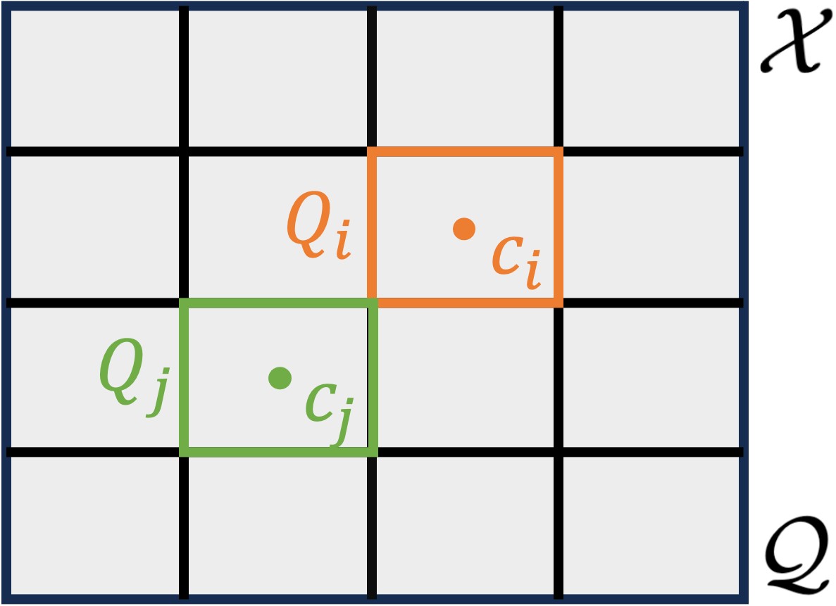
(a)

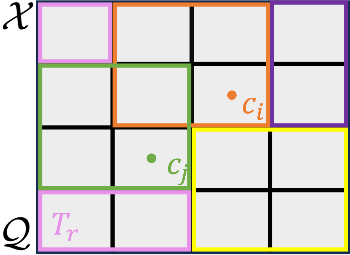
(b)

Figure 1: (a) Partition $\mathcal{Q}$ of the domain of interest $\mathcal{X}$, where $Q_{i}$ and $Q_{j}$ are two elements of the partition, $c_{i}$ and $c_{j}$ are the respective reference points. (b) Cover of target sets $\mathcal{T}$ of the partition $\mathcal{Q}$. Each color represents a different target set.

III-B Actions

Below we define actions linking a single abstract state to (possibly) a set of abstract states, named target set.

Let $\mathcal{T}=\{T_{i}\}_{i=1}^{M}$ be a finite collection of target sets covering $\mathcal{Q}$, in particular $\mathcal{T}\subseteq 2^{\mathcal{Q}}$, see Figure 1(b). Further, for every $i=1,...,M$, let $C_{i}$ be the set of reference states associated with $T_{i}$, that is $C_{i}=\bigcup_{Q\in T_{i}}\{\psi(R(x)):x\in Q\}$.

The collection of target sets defines the set of labelled abstract actions $\mathcal{A}=\{a_{r}:r=1,...,M\}$, where $a_{r}$ is associated with the target set $T_{r}$ as shown below. We construct the set of enabled actions at $s_{i}$ as follows.

Action $a_{r}$ is enabled at state $s_{i}$ if for every state $x_{k}\in R^{-1}(s_{i})$ there exists a control input $u_{k}$ such that the next state under nominal dynamics (3) belongs to the set of reference points associated with $T_{r}$, or, in other words, $\hat{x}_{k+1}\in C_{r}$. Formally, we define the (nominal) backward reachable set of a point $x^{\prime}\in\mathcal{X}$ as

$$\text{Pre}(x^{\prime}):=\{x\in\mathcal{X}:\exists u\in U,f(x,u)=x^{\prime}\}.$$ (5)

We slightly abuse notation and define analogously the (nominal) backward reachable set of a set $C_{r}\subset\mathcal{X}$ as

$$\text{Pre}(C_{r}):=\bigcup_{c_{j}\in C_{r}}\text{Pre}(c_{j}).$$ (6)

We require that backward reachable sets of reference points, or a union of those, can contain regions $Q_{i}$. Thus, we lay the following assumption.

Assumption 1

The backward reachable set of any reference point has a non-empty interior.

When the nominal dynamics is linear $f(x_{k},u_{k})=Ax_{k}+Bu_{k}$, Assumption 1 requires that the matrix $B$ is full rank.

Action $a_{r}$ is enabled at state $s_{i}$ iff $R^{-1}(s_{i})$ is contained in $\text{Pre}(C_{r})$, as shown in Figure 2(a):

$$R^{-1}(s_{i})\subseteq\text{Pre}(C_{r})\iff a_{r}\in\mathcal{A}(s_{i}).$$ (7)

In general for a continuous state such that $x\in\text{Pre}(C_{r})$ there may exist multiple control inputs leading to $C_{r}$, that is the sets $\{\text{Pre}(c_{j})\}_{c_{j}\in C_{r}}$ need not be disjoint. To unambiguously define a feedback controller $u:\mathcal{X}\rightarrow U$ we exploit the ordering of the partitioning sets $\{Q_{i}\}_{i=1}^{N}$ to assign a unique control input driving the state to $C_{r}$.

Let $c^{*}:\mathcal{X}\times\mathcal{A}\rightarrow\mathcal{X}$ be a function mapping a continuous state and abstract action to a continuous reference point indexed by the lowest integer, that is

$$c^{*}(x,a_{r}):= \operatorname*{arg\,min}_{c_{j}\in C_{r}}j \text{s.t.}\quad x\in\text{Pre}(c_{j}).$$ (8)

Let us define the unique control law $u^{*}:\mathcal{X}\times\mathcal{A}\rightarrow U$ as

$$u^{*}(x,a_{r}):=\{u:f(x,u)=c^{*}\}.$$ (9)

For every $C_{r}$, operation (8) naturally induces a partition on a set $R^{-1}(s_{i})$ satisfying (7), defined as

$$Q_{i}^{r}:=\{X\subseteq Q_{i}:\forall x,x^{\prime}\in X,c^{*}(x,a_{r})=c^{*}(x^{\prime},a_{r})\}.$$ (10)

In other words, the partition $Q_{i}^{r}=\{Q_{i,\ell}\}_{\ell=1}^{L_{r}}$ is a collection of $L_{r}$ non-overlapping regions of $Q_{i}$ defined by the points sharing the same next state under nominal dynamics under control law $u^{*}$, see Figure 2(b).

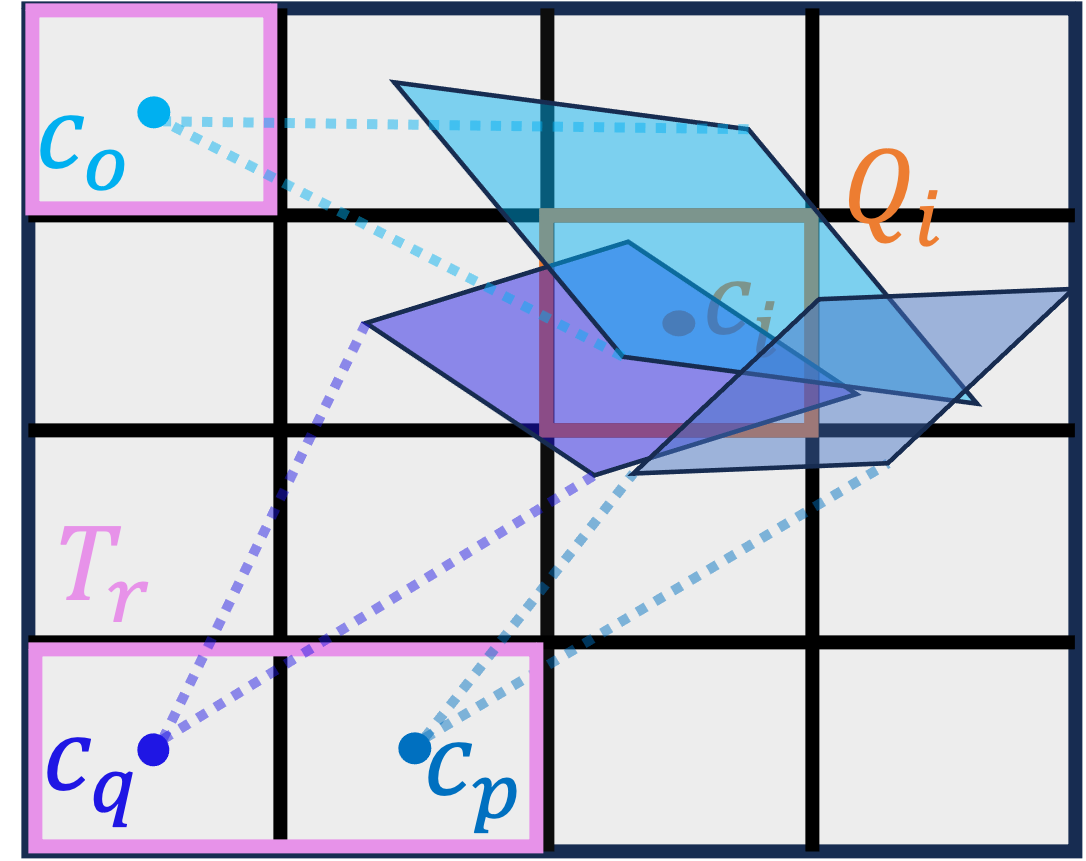
(a)

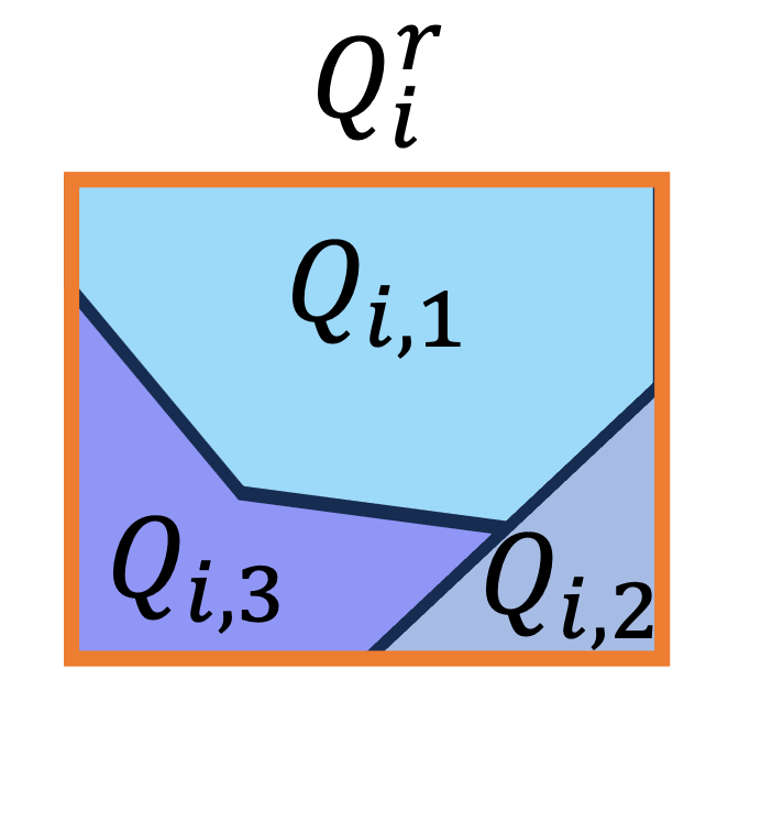
(b)

Figure 2: (a) $\text{Pre}(C_{r})$ represented as the union of $\text{Pre}(c_{o})$, $\text{Pre}(c_{p})$, and $\text{Pre}(c_{q})$; $a_{r}\in\mathcal{A}(s_{i})$ (b) Assuming the ordering $o<p<q$, the partition $Q_{i}^{r}$ induced on $Q_{i}$ by $C_{r}$.

III-C Transition Probabilities

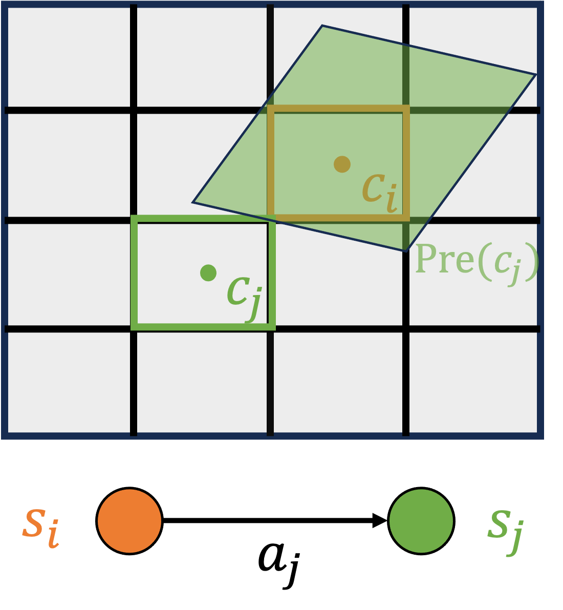
(a)

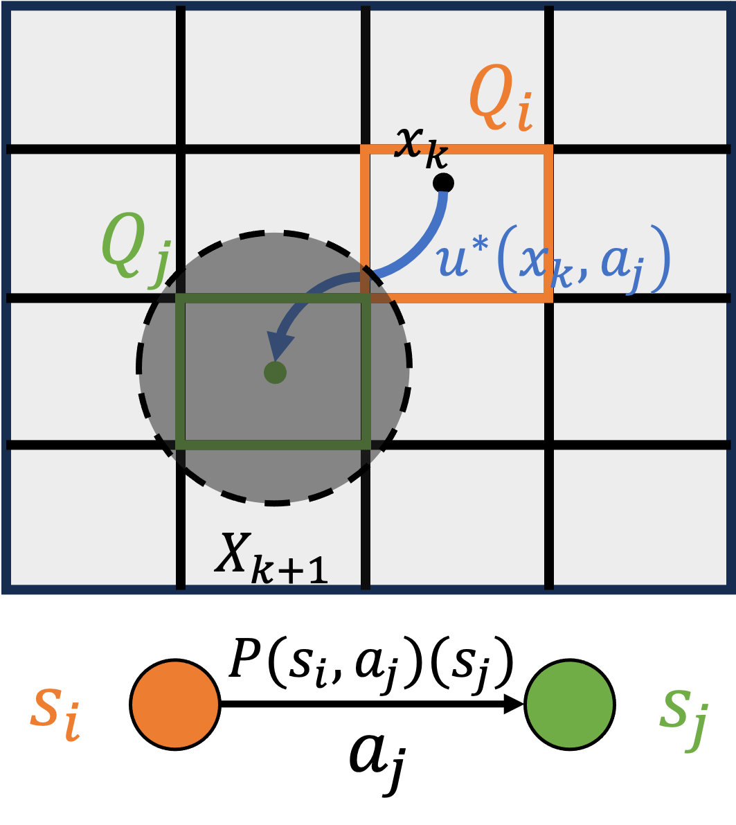
(b)

Figure 3: (a) Consider $T_{j}=Q_{j}$. If action $a_{j}\in\mathcal{A}(s_{i})$ then $\text{Pre}(c_{j})\supseteq Q_{i}$. (b) For every $x_{k}\in Q_{i}$ there exists an input $u_{k}=u^{*}(x,a_{j})$ driving the state to $c_{j}$. The shaded area represents the support of $T(dx_{k+1}|x_{k},u_{k})$.

In the remaining part of this section, we recall the construction scheme proposed by [2] to abstract a SDE with additive noise to an MDP and introduce a shortcoming of such a procedure. Suppose that the collection of target sets $\mathcal{T}$ coincides with the partition $\mathcal{Q}$, more precisely, $T_{r}=\{Q_{r}\}$ for every $r=1,...,N$. In this tailored setting we can simplify our discussion: every set $C_{r}$ contains a single element, namely $c_{r}$, hence action $a_{r}$ is enabled in the abstract state $s_{i}$ if and only if $R^{-1}(s_{i})\subseteq\text{Pre}(C_{r})=\text{Pre}(c_{r})$. Similarly, $Q_{i}^{r}$ is the trivial partition and contains a single element, namely $Q_{i}^{r}=\{Q_{i}\}$ – cfr. (10) – as depicted in Figure 3(a). A finite-state abstraction that describes this framework is an MDP $M=(S,\mathcal{A},P,R)$, where given $x_{k}\in R^{-1}(s_{i})$, an abstract action $a_{j}\in\mathcal{A}(s_{i}),$ and $u_{k}=u^{*}(x_{k},a_{j})$ the probability of transitioning to the abstract state $s_{j}$ can be computed as:

$$P(s_{i},a_{j})(s_{j}):=\int_{R^{-1}(s_{j})}T(dx_{k+1}|x_{k},u_{k}).$$ (11)

Due to the noise being additive (1) and given the control law $u^{*}$ we can express (11) as

$$P(s_{i},a_{j})(s_{j})=\mathbb{P}\{\omega\in\Omega:c_{j}+W_{k}(\omega)\in R^{-1}(s_{j})\},$$ (12)

where we have used the fact that under nominal dynamics $f(x_{k},u^{*}(x,a_{j}))=c_{j}$. This situation is depicted in Fig. 3(b).

III-D Shortcomings and Motivating Example

One shortcoming of this approach is that it may lead to a significant under-approximation of the dynamics of the concrete system. Formally expressed in (7), if $Q_{i}$ is not entirely contained in $\operatorname{Pre}(c_{j})$, $a_{j}$ is not enabled for $s_{i}$. As such, one may have to exclude a large set of actions if the dynamics are not well aligned with the chosen partition.

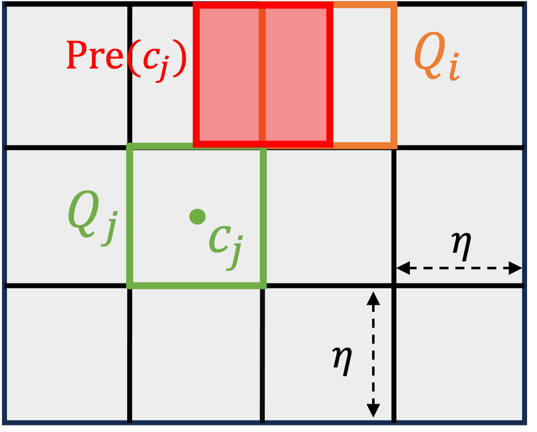
Figure 4: The dynamics are misaligned with the partition.

Example 1

Consider the SDE given by

$$X_{k+1}=X_{k}-u_{k}+W_{k},$$ (13)

where $X_{k}\in\mathbb{R}^{2}$, $W_{k}$ is a random variable taking values in $\mathbb{R}^{2}$, $u_{k}\in\mathcal{U}=[0,\eta]\times[\eta/2,3\eta/2]\subset\mathbb{R}^{2}$ for some $\eta>0$. Let the partition $\mathcal{Q}$ of $\mathcal{X}$ be a uniform grid such that each set $Q_{i}$ is a $\eta$ by $\eta$ box. Suppose that $\mathcal{T}=\mathcal{Q}$. Consider a reference state $c_{j}$, the center of the box $S_{j}$, and let us examine $\text{Pre}(T_{j})=\text{Pre}(c_{j})$: by inverting the nominal dynamics we can characterize such set as

$$\text{Pre}(c_{j})=\{x:\exists u\in\mathcal{U},c_{j}+u=x\},$$

which represents a copy of $S_{j}$ with its center shifted by $[\eta/2,\eta]$, as represented in Figure 4. Consequently, considering only one partition for each transition leads to an empty MDP: i.e., all abstract states $s_{i}$ have an empty action set. By considering a different target set, for instance partition $Q_{j}$ and its adjacent partition, it is easy to see that $Q_{i}$ is entirely contained in the union of the two $\operatorname{Pre}$ sets: this observation is the motivation to the following discussion.

IV Uncertain Transition Probabilities

In contrast to the previous discussion, let us consider now consider a general cover $\mathcal{T}$ of the partition $\mathcal{Q}$. , i.e. at least one out of the $M$ target sets, say $T_{r}$, contains more than one element of $\mathcal{Q}$; equivalently, $C_{r}$ contains more than one reference state. Let $Q_{i}\subseteq\text{Pre}(C_{r})$, as depicted in Figure 2(a), and consider the non-trivial partition $Q_{i}^{r}=\{Q_{i,\ell}\}_{\ell=1}^{L_{r}}$ induced on $Q_{i}$ by (8) and described by (10). We know that for every $\ell=1,...,L_{r}$ and for every $x\in Q_{i,\ell}$ there exists a control law that can drive the state to the center of one of the reference points in $C_{r}$, namely $u^{*}(x,a_{r})$.

Naturally, in this new setting, it is not possible to describe the transition from $s_{i}$ under action $a_{r}$ to a future abstract state $s_{j}=R(c)$ for $c\in T_{r}$ by a single transition probability function as in (12), but rather by a set of transition probability functions. Indeed, the probability of reaching $s_{j}$ from $s_{i}$ under action $a_{r}$ depends on the actual continuous state $x\in Q_{i}$ from which the transition takes place.

In order to encompass this framework, we define an uncertain probability transition function $P_{\mathrel{\mathchoice{\vbox to3.01389pt{\hbox{$\displaystyle.$}\vss\hbox{$\displaystyle.$}\vss\hbox{$\displaystyle.$}}}{\vbox to3.01389pt{\hbox{$\textstyle.$}\vss\hbox{$\textstyle.$}\vss\hbox{$\textstyle.$}}}{\vbox to2.10971pt{\hbox{$\scriptstyle.$}\vss\hbox{$\scriptstyle.$}\vss\hbox{$\scriptstyle.$}}}{\vbox to1.50694pt{\hbox{$\scriptscriptstyle.$}\vss\hbox{$\scriptscriptstyle.$}\vss\hbox{$\scriptscriptstyle.$}}}}}$ which encapsulates all possible cases and captures the nondeterminism introduced by clustering multiple reference points. Consider an abstract state $s_{i}$, an action $a_{r}\in\mathcal{A}(s_{i})$, the partitioning $Q_{i}^{r}$, and suppose that $x_{k}\in Q_{i,\ell}$ for some $\ell\in\{1,...,L_{r}\}$: under the control input $u_{k}=u^{*}(x_{k},a_{r})$ the next state under nominal dynamics is the reference point $c^{*}(x,a_{r})\in C_{r}$. Let us define

$$P^{\ell}(s_{i},a_{r})(s_{j}):=\int_{R^{-1}(s_{j})}T(dx_{k+1}|x_{k},u_{k}),$$ (14)

By enumerating $\ell=1,...,L_{r}$ we obtain a set of transition probability functions which describes all cases, namely $x\in Q_{i,1},...,x\in Q_{i,L_{r}}$. Accordingly, we define the RMDP $M_{\mathrel{\mathchoice{\vbox to3.01389pt{\hbox{$\displaystyle.$}\vss\hbox{$\displaystyle.$}\vss\hbox{$\displaystyle.$}}}{\vbox to3.01389pt{\hbox{$\textstyle.$}\vss\hbox{$\textstyle.$}\vss\hbox{$\textstyle.$}}}{\vbox to2.10971pt{\hbox{$\scriptstyle.$}\vss\hbox{$\scriptstyle.$}\vss\hbox{$\scriptstyle.$}}}{\vbox to1.50694pt{\hbox{$\scriptscriptstyle.$}\vss\hbox{$\scriptscriptstyle.$}\vss\hbox{$\scriptscriptstyle.$}}}}}=(S,\mathcal{A},P_{\mathrel{\mathchoice{\vbox to3.01389pt{\hbox{$\displaystyle.$}\vss\hbox{$\displaystyle.$}\vss\hbox{$\displaystyle.$}}}{\vbox to3.01389pt{\hbox{$\textstyle.$}\vss\hbox{$\textstyle.$}\vss\hbox{$\textstyle.$}}}{\vbox to2.10971pt{\hbox{$\scriptstyle.$}\vss\hbox{$\scriptstyle.$}\vss\hbox{$\scriptstyle.$}}}{\vbox to1.50694pt{\hbox{$\scriptscriptstyle.$}\vss\hbox{$\scriptscriptstyle.$}\vss\hbox{$\scriptscriptstyle.$}}}}},R_{\mathrel{\mathchoice{\vbox to3.01389pt{\hbox{$\displaystyle.$}\vss\hbox{$\displaystyle.$}\vss\hbox{$\displaystyle.$}}}{\vbox to3.01389pt{\hbox{$\textstyle.$}\vss\hbox{$\textstyle.$}\vss\hbox{$\textstyle.$}}}{\vbox to2.10971pt{\hbox{$\scriptstyle.$}\vss\hbox{$\scriptstyle.$}\vss\hbox{$\scriptstyle.$}}}{\vbox to1.50694pt{\hbox{$\scriptscriptstyle.$}\vss\hbox{$\scriptscriptstyle.$}\vss\hbox{$\scriptscriptstyle.$}}}}})$ where

$$P_{\mathrel{\mathchoice{\vbox to3.01389pt{\hbox{$\displaystyle.$}\vss\hbox{$\displaystyle.$}\vss\hbox{$\displaystyle.$}}}{\vbox to3.01389pt{\hbox{$\textstyle.$}\vss\hbox{$\textstyle.$}\vss\hbox{$\textstyle.$}}}{\vbox to2.10971pt{\hbox{$\scriptstyle.$}\vss\hbox{$\scriptstyle.$}\vss\hbox{$\scriptstyle.$}}}{\vbox to1.50694pt{\hbox{$\scriptscriptstyle.$}\vss\hbox{$\scriptscriptstyle.$}\vss\hbox{$\scriptscriptstyle.$}}}}}(s_{i},a_{r})(s_{j})=\bigcup_{\ell=1}^{L_{r}}P^{\ell}(s_{i},a_{r})(s_{j}).$$ (15)

This is shown graphically in Figure 5(a) and Figure 5(b).

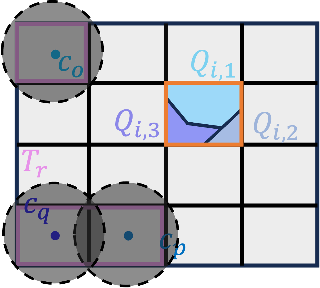
(a)

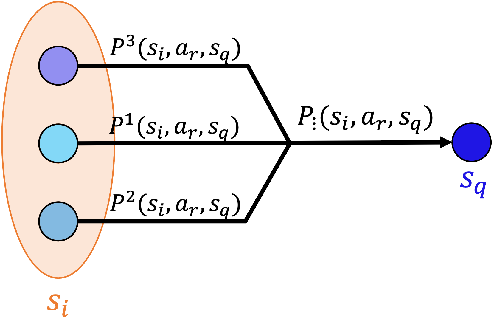
(b)

Figure 5: (a) Computation of $P^{\ell}(s_{i},a_{r})(s_{q})$ as per (14) for $\ell=1,2,3$. (b) Uncertain transition probability function from a state $s_{i}$ to a state $s_{q}$ under action $a_{r}$.

Remark 3

The target sets can be selected by inspection of the backward reachable set. An intuitive choice is to select adjacent cells, creating ‘neighborhoods’ of increasing size.

V PAC Probability Intervals via Sampling

Computing (14) is possible only when the distribution of the additive noise $W_{k}$ is perfectly known. Additionally, even if it were known, computing explicitly the integral could be difficult or undesirable in certain cases. Instead we provide a lower and upper bound of $P^{\ell}(s_{i},a_{r})(s_{j})$ using the sampling-and-discarding scenario approach proposed in [6] and improved in [18]. In particular, we adopt the framework presented in [2], under the following necessary assumption

Assumption 2 (Non-degeneracy)

For every $k$, $W_{k}$ has a density with respect to the Lebesgue measure.

We summarize the results therein here. Let us collect a set of $Z\in\mathbb{N}$ i.i.d. samples of $W_{k}$, denoted $w_{k}^{(1)},...,w_{k}^{(Z)}$ and define the quantities

$$Z_{s_{j}}^{\text{in}} =|\{w_{k}^{(i)}:w_{k}^{(i)}+c_{j}\in Q_{j}\}|,\quad Z_{s_{j}}^{\text{out}} =Z-Z_{s_{j}}^{\text{in}}.$$

In words, $Z_{s_{j}}^{\text{in}}$ is the number of samples $w_{k}^{(i)}$ which, when shifted by $c_{j}$, fall within region $Q_{j}$.

Theorem 1

(PAC probability intervals [2, Theorem 1]) Given $Z$ samples of the noise $W_{k}$, compute $Z_{s_{j}}^{\text{out}}$ and fix a confidence parameter $\beta$. It holds that

$$\mathbb{P}^{Z}\{{\underline{p}_{j,\ell}}\leq P^{\ell}(s_{i},a_{r})(s_{j})\leq{\overline{p}_{j,\ell}}\}\geq 1-\beta,$$

where ${\underline{p}_{j,\ell}}=0$ if $Z_{s_{j}}^{\text{out}}=Z$; otherwise ${\underline{p}_{j,\ell}}$ is the solution of

$$\frac{\beta}{2Z}=\sum_{i=0}^{Z_{s_{j}}^{\text{out}}}{Z\choose i}(1-{\underline{p}_{j,\ell}})^{i}{\underline{p}_{j,\ell}}^{Z-i},$$

and ${\overline{p}_{j,\ell}}=1$ if $Z_{s_{j}}^{\text{out}}=0$; otherwise ${\overline{p}_{j,\ell}}$ is the solution of

$$\frac{\beta}{2Z}=1-\sum_{i=0}^{Z_{s_{j}}^{\text{out}}-1}{Z\choose i}(1-{\overline{p}_{j,\ell}})^{i}{\overline{p}_{j,\ell}}^{Z-i}.$$

Theorem 1 allows us to provide an upper and lower bound on the individual transition probabilities $P^{\ell}(s_{i},a_{r},s_{j})$.

We can then describe the resulting abstraction as a RMDP $M_{\mathrel{\mathchoice{\vbox to3.01389pt{\hbox{$\displaystyle.$}\vss\hbox{$\displaystyle.$}\vss\hbox{$\displaystyle.$}}}{\vbox to3.01389pt{\hbox{$\textstyle.$}\vss\hbox{$\textstyle.$}\vss\hbox{$\textstyle.$}}}{\vbox to2.10971pt{\hbox{$\scriptstyle.$}\vss\hbox{$\scriptstyle.$}\vss\hbox{$\scriptstyle.$}}}{\vbox to1.50694pt{\hbox{$\scriptscriptstyle.$}\vss\hbox{$\scriptscriptstyle.$}\vss\hbox{$\scriptscriptstyle.$}}}}}=(S,\mathcal{A},P_{\mathrel{\mathchoice{\vbox to3.01389pt{\hbox{$\displaystyle.$}\vss\hbox{$\displaystyle.$}\vss\hbox{$\displaystyle.$}}}{\vbox to3.01389pt{\hbox{$\textstyle.$}\vss\hbox{$\textstyle.$}\vss\hbox{$\textstyle.$}}}{\vbox to2.10971pt{\hbox{$\scriptstyle.$}\vss\hbox{$\scriptstyle.$}\vss\hbox{$\scriptstyle.$}}}{\vbox to1.50694pt{\hbox{$\scriptscriptstyle.$}\vss\hbox{$\scriptscriptstyle.$}\vss\hbox{$\scriptscriptstyle.$}}}}},R_{\mathrel{\mathchoice{\vbox to3.01389pt{\hbox{$\displaystyle.$}\vss\hbox{$\displaystyle.$}\vss\hbox{$\displaystyle.$}}}{\vbox to3.01389pt{\hbox{$\textstyle.$}\vss\hbox{$\textstyle.$}\vss\hbox{$\textstyle.$}}}{\vbox to2.10971pt{\hbox{$\scriptstyle.$}\vss\hbox{$\scriptstyle.$}\vss\hbox{$\scriptstyle.$}}}{\vbox to1.50694pt{\hbox{$\scriptscriptstyle.$}\vss\hbox{$\scriptscriptstyle.$}\vss\hbox{$\scriptscriptstyle.$}}}}})$ where

$$P_{\mathrel{\mathchoice{\vbox to3.01389pt{\hbox{$\displaystyle.$}\vss\hbox{$\displaystyle.$}\vss\hbox{$\displaystyle.$}}}{\vbox to3.01389pt{\hbox{$\textstyle.$}\vss\hbox{$\textstyle.$}\vss\hbox{$\textstyle.$}}}{\vbox to2.10971pt{\hbox{$\scriptstyle.$}\vss\hbox{$\scriptstyle.$}\vss\hbox{$\scriptstyle.$}}}{\vbox to1.50694pt{\hbox{$\scriptscriptstyle.$}\vss\hbox{$\scriptscriptstyle.$}\vss\hbox{$\scriptscriptstyle.$}}}}}(s_{i},a_{r})(s_{j}):=\bigcup_{\ell=1}^{L_{r}}[{\underline{p}_{j,\ell}},{\overline{p}_{j,\ell}}].$$ (16)

In order to leverage existing algorithms for value iteration on iMDPs, following the approach in [13, 11], we can embed (abstract) the resulting RMDP into an iMDP $M_{\updownarrow}=(S,\mathcal{A},P_{\updownarrow},R)$ where the uncertain transition probability from $s_{i}$ to state $s_{j}$ under action $a_{r}$ is defined as

$$P_{\updownarrow}(s_{i},a_{r})(s_{j})=[\underline{p}_{j},\overline{p}_{j}],$$ (17)

where $\underline{p}_{j}=\min P_{\mathrel{\mathchoice{\vbox to3.01389pt{\hbox{$\displaystyle.$}\vss\hbox{$\displaystyle.$}\vss\hbox{$\displaystyle.$}}}{\vbox to3.01389pt{\hbox{$\textstyle.$}\vss\hbox{$\textstyle.$}\vss\hbox{$\textstyle.$}}}{\vbox to2.10971pt{\hbox{$\scriptstyle.$}\vss\hbox{$\scriptstyle.$}\vss\hbox{$\scriptstyle.$}}}{\vbox to1.50694pt{\hbox{$\scriptscriptstyle.$}\vss\hbox{$\scriptscriptstyle.$}\vss\hbox{$\scriptscriptstyle.$}}}}}(s_{i},a_{r})(s_{j})$ and $\overline{p}_{j}=\max P_{\mathrel{\mathchoice{\vbox to3.01389pt{\hbox{$\displaystyle.$}\vss\hbox{$\displaystyle.$}\vss\hbox{$\displaystyle.$}}}{\vbox to3.01389pt{\hbox{$\textstyle.$}\vss\hbox{$\textstyle.$}\vss\hbox{$\textstyle.$}}}{\vbox to2.10971pt{\hbox{$\scriptstyle.$}\vss\hbox{$\scriptstyle.$}\vss\hbox{$\scriptstyle.$}}}{\vbox to1.50694pt{\hbox{$\scriptscriptstyle.$}\vss\hbox{$\scriptscriptstyle.$}\vss\hbox{$\scriptscriptstyle.$}}}}}(s_{i},a_{r})(s_{j})$.

It is obvious from (16) and (17) that the collection of MDPs described by $M_{\mathrel{\mathchoice{\vbox to3.01389pt{\hbox{$\displaystyle.$}\vss\hbox{$\displaystyle.$}\vss\hbox{$\displaystyle.$}}}{\vbox to3.01389pt{\hbox{$\textstyle.$}\vss\hbox{$\textstyle.$}\vss\hbox{$\textstyle.$}}}{\vbox to2.10971pt{\hbox{$\scriptstyle.$}\vss\hbox{$\scriptstyle.$}\vss\hbox{$\scriptstyle.$}}}{\vbox to1.50694pt{\hbox{$\scriptscriptstyle.$}\vss\hbox{$\scriptscriptstyle.$}\vss\hbox{$\scriptscriptstyle.$}}}}}$ is a subset of the MDPs described by $M_{\updownarrow}$. Indeed if $P\in P_{\mathrel{\mathchoice{\vbox to3.01389pt{\hbox{$\displaystyle.$}\vss\hbox{$\displaystyle.$}\vss\hbox{$\displaystyle.$}}}{\vbox to3.01389pt{\hbox{$\textstyle.$}\vss\hbox{$\textstyle.$}\vss\hbox{$\textstyle.$}}}{\vbox to2.10971pt{\hbox{$\scriptstyle.$}\vss\hbox{$\scriptstyle.$}\vss\hbox{$\scriptstyle.$}}}{\vbox to1.50694pt{\hbox{$\scriptscriptstyle.$}\vss\hbox{$\scriptscriptstyle.$}\vss\hbox{$\scriptscriptstyle.$}}}}}$ it implies that $P\in P_{\updownarrow}$. Let $\pi^{*}$ denote the optimal policy for $M_{\updownarrow}$. It follows that

$$\min_{P\in P_{\updownarrow}}\mathbb{P}^{\pi^{*}}_{P}\{\varphi^{\prime K}_{s_{0}}\}\leq\min_{P\in P_{\mathrel{\mathchoice{\vbox to2.15277pt{\hbox{$\displaystyle.$}\vss\hbox{$\displaystyle.$}\vss\hbox{$\displaystyle.$}}}{\vbox to2.15277pt{\hbox{$\textstyle.$}\vss\hbox{$\textstyle.$}\vss\hbox{$\textstyle.$}}}{\vbox to1.50694pt{\hbox{$\scriptstyle.$}\vss\hbox{$\scriptstyle.$}\vss\hbox{$\scriptstyle.$}}}{\vbox to1.07639pt{\hbox{$\scriptscriptstyle.$}\vss\hbox{$\scriptscriptstyle.$}\vss\hbox{$\scriptscriptstyle.$}}}}}}\mathbb{P}^{\pi^{*}}_{P}\{\varphi^{\prime K}_{s_{0}}\}.$$

This embedding allows us to employ existing tools to obtain a policy with a valid lower bound on the probability of satisfaction of the reach-avoid property for the RMDP. Note that we compute the optimal policy $\pi^{*}$ with respect to the iMDP, which in general differs from the optimal policy with respect to the RMDP. We leave this for future work.

We conclude this section by enunciating the following theorem connecting the probability of satisfaction of the reach-avoid property on the iMDP given an optimal policy with the probability of satisfaction of the reach-avoid property on the underlying dynamical system by refining the policy to a feedback controller. The proof follows the rationale in [1, Theorem 2], and is omitted for brevity.

Theorem 2 (Adapted from [1])

Let $\pi^{*}$ denote the optimal policy (4) for the iMDP obtained according to $\eqref{eq:embedding-to-imdp}$, and let $L_{\max}=\max_{r}L_{r}$. For $\alpha:=\beta NML_{\max}$ and for the controller defined by $\phi:=u^{*}(x,\pi^{*}(R(x),k))$ it holds

$$\min_{P\in P_{\updownarrow}}\mathbb{P}^{\pi^{*}}_{P}\{\varphi^{\prime K}_{s_{0}}\}\geq\eta\Rightarrow\mathbb{P}^{N}\{\mathbb{P}^{\phi}\{\varphi^{K}_{x_{0}}\geq\eta\}\}\geq 1-\alpha.$$ (18)

VI Experimental Evaluation

Our codebase is based upon [1], which for brevity is denoted as “single-target procedure” (STP), and has been modified in order to include multiple-target transitions (hence denoted as MTP). The controller synthesis uses the probabilistic model checker PRISM [14] to compute optimal iMDP policies. Each interval transition probability is computed using $N=20000$ samples and a confidence $\beta=10^{-8}$.

Example 1 (Cont’d). Let us consider the dynamical model (13), over the domain $\mathcal{X}=[-25,25]^{2}$, partitioned into 2500 square regions, where the goal set is the region $\mathcal{X}_{G}=[-25,25]\times[-25,-24]$. The control input lies in the set $\mathcal{U}=[0,1]\times[0.5,1.5]$, and the noise follows a Gaussian distribution $W_{k}\sim\mathcal{N}(0,0.15\cdot I)$. Our goal is the computation of a control policy making the dynamics reach the goal in 50 time steps at most. As outlined in Example 1, the STP returns an iMDP with no actions enabled. We thus select target sets composed of two adjacent partitions, so that the composite $\operatorname{Pre}$ set covers an entire partition region. Our procedure creates an iMDP equipped with 42391 transitions, and computes a policy whose lower bounds on the satisfaction probability is shown in Fig. 6, with a confidence (see (18)) $\alpha\simeq 0.12$.

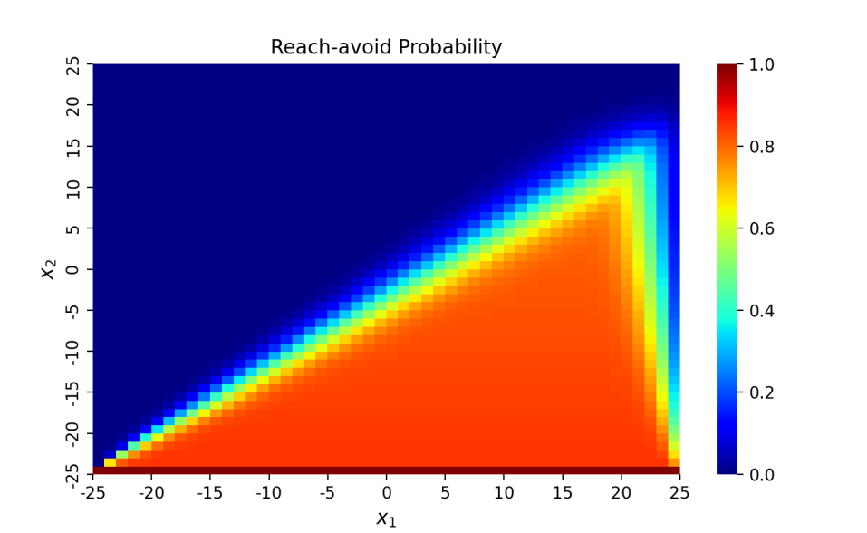
Figure 6: Lower bound on the probability of reaching the goal set (represented by the lowest row of states) for Example 1.

Double Integrator. Let us consider the stochastic model

$$X_{k+1}=\begin{bmatrix}1&1\\ 0&1\end{bmatrix}X_{k}+\begin{bmatrix}0.5&0\\ 0&1\end{bmatrix}u_{k}+W_{k},$$ (19)

where $W_{k}\sim\mathcal{N}(0,0.15\cdot I)$. The reach-avoid task is to reach set $[-2,2]^{2}$ within 5 time steps, while avoiding states $X\notin[-11,11]^{2}$. The control input is limited by the set $[-2,4]\times[-3,3]$. We partition the domain $\mathcal{X}=[-11,11]^{2}$ into square partitions, in four different configurations: 11x11, 15x15, 18x18, 20x20 regions. We consider target sets composed of two adjacent regions. The complete results are reported in Table I, in terms of computational time, number of transitions of the resulting abstractions, and in percentage of states with a positive probability of reaching the goal set, along with the confidence $\alpha$ (see (18)) for the MTP approach. The first two partitioning choices return an empty iMDP when considering the STP, as the $\operatorname{Pre}$ of a region is not entirely contained in any single partition, whilst the MTP successfully construct an iMDP. Starting from the case of 18x18 partitions and up, the STP returns smaller abstractions than the MTP; this is expected, as the MTP implicitly considers significantly more target partitions – this behaviour is reflected in the higher computational times needed to construct the abstract models. We notice that the MTP has a higher percentage of states with a positive probability of reaching the goal set, as it is equipped with more transitions compared to the STP. Further, as the partitions’ number increases, and thus the partitions’ size narrows, the gap between the STP and the MTP shrinks: the abstraction becomes finer for both procedures, providing a more precise depiction of the concrete underlying system.

Partition	Transitions		Time [s]		Reach [%]		$\alpha$
	STP	MTP	STP	MTP	STP	MTP	MTP
$11^{2}$	–	1907	–	7.9	–	61.9	0.0006
$15^{2}$	–	5592	–	11.2	–	62.2	0.002
$18^{2}$	6423	26511	8.4	28.6	54.3	66.0	0.01
$20^{2}$	13155	52580	9.8	35.1	62.5	68.5	0.03
$22^{2}$	22422	90896	11.5	43.7	61.1	66.9	0.05

Table I: Comparison between the STP and MTP abstractions, in terms of number of transitions, computational time, and percentage of states that have a positive probability to reach the goal set, and confidence $\alpha$ for the MTP.

VII Discussion and Conclusions

We have developed a novel abstraction procedure for discrete-time stochastic systems, exploiting nondeterministic transitions to generate finite-state abstract models. By allowing each transition to reach a set of partitions, rather than a single region, we show that we can build an abstraction even when the backward reach set does not entirely cover any single partition region, thus generalising the scope of earlier results. This event can occur for systems whose input set is constrained (e.g. with significant saturation): thus, our approach is suited for control designs with performance costs. Our experimental evidence shows that this flexibility comes at the cost of generating larger (in terms of transitions) models than the existing single-target approach, and hence introducing more behaviours in the abstraction. The selection of target sets and the embedding of an RMDP into an iMDP affect the performance of our method: as such, a deeper study of tailored algorithms for RMDPs which exploit the structure of the uncertain transition function obtained by this scheme are matter of future efforts.

References

- [1] T. Badings, L. Romao, A. Abate, and N. Jansen. Probabilities are not enough: formal controller synthesis for stochastic dynamical systems with epistemic uncertainty. In AAAI Conference On Artificial Intelligence. AAAI, 2023.
- [2] T. Badings, L. Romao, A. Abate, D. Parker, H. Poonawala, M. Stoelinga, and N. Jensen. Robust control for dynamical systems with non-Gaussian via formal abstractions. Journal of Artificial Intelligence Research. To appear, 2023.
- [3] C. Baier and J.-P. Katoen. Principles of model checking. MIT press, 2008.
- [4] A. Banse, L. Romao, A. Abate, and R. Jungers. Data-driven memory-dependent abstractions of dynamical systems. In Learning for Dynamics and Control Conference, pages 891–902. PMLR, 2023.
- [5] A. Banse, L. Romao, A. Abate, and R. M. Jungers. Data-driven abstractions via adaptive refinements and a Kantorovich metric. In 2023 62nd IEEE Conference on Decision and Control (CDC), pages 6038–6043. IEEE, 2023.
- [6] M. C. Campi and S. Garatti. A sampling-and-discarding approach to chance-constrained optimization: feasibility and optimality. Journal of optimization theory and applications, 148(2):257–280, 2011.
- [7] R. Coppola, A. Peruffo, and M. Mazo Jr. Data-driven abstractions for verification of deterministic systems. arXiv preprint arXiv:2211.01793, 2022.
- [8] R. Coppola, A. Peruffo, and M. Mazo Jr. Data-driven abstractions for verification of linear systems. IEEE Control Systems Letters, 2023.
- [9] R. Coppola, A. Peruffo, and M. Mazo Jr. Data-driven abstractions for control systems, 2024.
- [10] M. Cubuktepe, N. Jansen, S. Junges, J.-P. Katoen, and U. Topcu. Scenario-based verification of uncertain mdps. In International Conference on Tools and Algorithms for the Construction and Analysis of Systems, pages 287–305. Springer, 2020.
- [11] T. Dean, R. Givan, and S. Leach. Model reduction techniques for computing approximately optimal solutions for markov decision processes. In Proceedings of the Thirteenth conference on Uncertainty in artificial intelligence, pages 124–131, 1997.
- [12] A. Devonport, A. Saoud, and M. Arcak. Symbolic abstractions from data: A pac learning approach. In 2021 60th IEEE Conference on Decision and Control (CDC), pages 599–604. IEEE, 2021.
- [13] R. Givan, S. Leach, and T. Dean. Bounded-parameter markov decision processes. Artificial Intelligence, 122(1):71–109, 2000.
- [14] M. Kwiatkowska, G. Norman, and D. Parker. Prism 4.0: Verification of probabilistic real-time systems. In Computer Aided Verification: 23rd International Conference, CAV 2011, Snowbird, UT, USA, July 14-20, 2011. Proceedings 23, pages 585–591. Springer, 2011.
- [15] A. Lavaei, S. Soudjani, E. Frazzoli, and M. Zamani. Constructing mdp abstractions using data with formal guarantees. IEEE Control Systems Letters, 2022.
- [16] A. Peruffo and M. Mazo Jr. Data-driven abstractions with probabilistic guarantees for linear petc systems. IEEE Control Systems Letters, 2022.
- [17] A. Peruffo and M. Mazo Jr. Sampling performance of periodic event-triggered control systems: a data-driven approach. IEEE Transactions on Control of Networked Systems, to appear, 2023.
- [18] L. Romao, A. Papachristodoulou, and K. Margellos. On the exact feasibility of convex scenario programs with discarded constraints. IEEE Transactions on Automatic Control, 68(4):1986–2001, 2022.
- [19] P. Tabuada. Verification and control of hybrid systems: a symbolic approach. Springer Science & Business Media, 2009.