Quantum integrated sensing and communication via entanglement
Abstract
Quantum communication and quantum metrology are widely compelling applications in the field of quantum information science, and quantum remote sensing is an intersection of both. Despite their differences, there are notable commonalities between quantum communication and quantum remote sensing, as they achieve their functionalities through the transmission of quantum states. Here we propose a novel quantum integrated sensing and communication (QISAC) protocol, which achieves quantum sensing under the Heisenberg limit while simultaneously enabling quantum secure communication through the transmission of entanglements. We have theoretically proven its security against eavesdroppers. The security of QISAC is characterized by the secrecy capacity for information bit as well as asymmetric Fisher information gain for sensing. Through simulations conducted under the constraints of limited entanglement resources, we illustrate that QISAC maintains high accuracy in the estimation of phase. Hence our QISAC offers a fresh perspective for the applications of future quantum networks.
I Introduction
Information science has embarked on a revolutionary step with the integration of quantum properties, where quantum secure communication and metrology are major breakthroughs of quantum information science. Relying on the quantum entanglement as a core resource [1], cryptography or communication paradigms with information-theoretic security, such as quantum key distribution [2], quantum secret sharing [3, 4], and quantum secure direct communication (QSDC) [5], have been established. QSDC enables secure and reliable transmission of private messages in quantum channels susceptible to eavesdropping and noise [6, 7, 8, 9, 10, 11, 12], with high-capacity features [13, 14, 15]. Leveraging the violation of the Bell-inequality, it achieves device-independent security, meaning secure communication can be achieved without trusting the inner workings of communication devices [16]. Experimental results have shown that they can connect legitimate users to achieve on-demand information sharing [17, 18] and realize a multi-user quantum information network [19].
Quantum metrology [20, 21, 22, 23, 24, 25] is an another practical application of quantum physics, involves utilizing quantum systems for parameter estimation. The entanglement and superposition of quantum states have been demonstrated to enhance the sensitivity of parameter estimation. Theoretically, a quantum entangled sensor has the potential to surpass the standard quantum limit (SQL) of any classical sensor, and achieve measurement precision approaching the Heisenberg limit (HL), where the variance of the estimated parameter decreases from being proportional to to being proportional to . Although most quantum metrology protocols rely on multipartite entangled states, such as the NOON states, the constraints posed by quantum hardware in the noisy intermediate-scale quantum (NISQ) era [26] limit the practical applicability of these protocols, thereby increasing resource requirements.
A suitable alternative is the bipartite entangled state, such as the Bell state, which is the quantum state adopted by most quantum remote sensing (QRS) protocols [27, 28]. Similar to blind quantum computing achieved through the integration of quantum computing and quantum cryptography, the intersection of quantum cryptography and quantum metrology has led to the emergence of QRS. The concept of a quantum sensor network is gaining momentum in quantum metrology, with quantum cryptography playing a significant role in protecting sensing data during transmission. QRS protocols employ random quantum states to enhance the security of sensing parameters between separate remote nodes, whose security level is determined by the probability of detecting Eve’s cheating. Through QRS schemes, one can achieve precise sensing of a remote system beyond the standard quantum limit while simultaneously ensuring the transmission of sensing parameters with quantum-native security. Specifically, users can implement secure QRS scheme by sharing photon pairs in Bell states between local and remote sites [27], where the security level is characterized by asymmetric Fisher information gain. Most recently, a quantum secure metrology protocol was constructed using bipartite entanglement pairs to provide high security and discussed the precision-security trade-off in a scenario with finite entanglement sources [28].
If taking a unified perspective on communication and sensing, we might integrate communication and sensing functionalities into a single system. This dual functionality can utilize resources more effectively. The introduction of quantum properties will further enhance the security of communication and sensing, as well as the precision of sensing. Finally, generating a novel information processing infrastructure.
Against this background, we propose a quantum integrated sensing and communication (QISAC) protocol, implementing simultaneous quantum sensing and QSDC, rather than building separate sensing and communication systems. In such a protocol, the sensing transcends the standard quantum limit and attains measurement precision approaching the Heisenberg limit, while the communication maintains a positive secrecy capacity under collective attacks by Eve.
The paper is organized as follows. In Sec. II, we present the modified entanglement-based QSDC protocol and fundamental concepts in quantum metrology. In Sec. III, we detail the proposed QISAC scheme, demonstrating that the QISAC protocol can achieve the Heisenberg limit in parameter sensing. In Sec. IV, we provide a security proof for the proposed QISAC protocol from both quantum sensing and quantum communication perspectives. Based on the physical structure, we simulate the performance of QISAC. Finally, we draw conclusions and provide an outlook in Sec. VI.
II Elements
II.1 Modified two-step QSDC protocol
In the two-step QSDC scheme [6], legitimate users Alice and Bob employ the following Einstein-Podolsky-Rosen (EPR) states to achieve the secure transmission of private information:
| (1) | ||||
They establish a consensus on the particular mapping of the , , , and states to the classical two-bit classical information 00, 01, 10, and 11, respectively. By enhancing the eavesdropping detection part, the modified two-step protocol can resist malicious party [29] secuely. As shown in Fig. 1, the detail steps of this entanglement-based QSDC protocol are as follows.
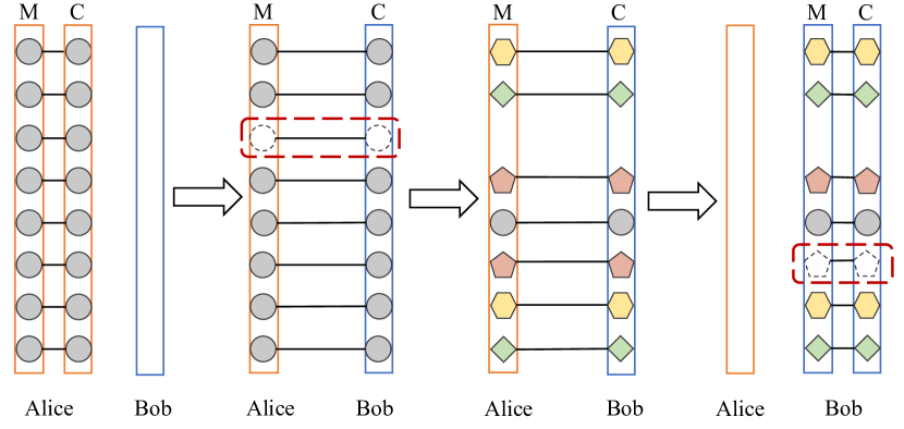
Step 1, states preparation. Alice prepares an ordered sequence of EPR pairs in state and divides the sequence into two particle sequences. One of them is called the checking sequence or simply the C sequence. The remaining EPR partner particles consist of the other message-coding sequence and is called the M sequence for short.
Step 2, qubits transmission and first eavesdropping detection. The C sequence is sent from Alice to Bob. Bob randomly selects some particles from the C sequence and measures them using the bases , or randomly. Bob informs Alice of the positions and measurement bases of the chosen particles. Alice performs the same measurements on the corresponding partner particles in the M sequence and checks the results with Bob. They calculate the quantum bit error rate (QBER) and determine that no eavesdropper is interfering with the quantum channel, if the QBER is below the tolerance threshold. Otherwise, they terminate their communication.
Step 3, encoding. Alice applies one of the following four unitary operators to each particles in the M sequence to encode 00, 01, 10, 11, respectively,
| (2) | ||||
Particularly, Alice has to apply a small trick within the M sequence for the second eavesdropping detection. She randomly selects certain particles as samples to perform one of the four unitary operators disorderly. These states do not carry valuable information; instead, random numbers are associated with them.
Step 4, measurement and the second eavesdropping detection. Upon receiving the M sequence, Bob combines it with the other sequence and performs the Bell-state measurement. Alice informs Bob about the positions of the sampling states and the specific unitary operators applied. By checking the chosen sampling pairs, Bob estimates the QBER within the M sequence transmission. If the QBER is reasonably low, Alice and Bob can trust the process. If not, they will abandon the transmission and revert to step 1. Ultimately, Bob retrieves the message bits transmitted by Alice.
Considering the depolarizing channel, we derive the lower bound of secrecy capacity for the modified two-step QSDC protocol based on [30]. Specifically, we have
| (3) |
where is four-array Shonnon entropy, is the Shannon entropy, and are the reception rates of Bob and Eve respectively, and e is the error rate distribution of the main channel.
II.2 Quantum metrology
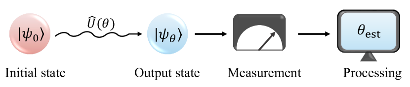
In the field of quantum metrology, a fundamental task is estimating small parameters by measuring the expectation value of a Hermitian operator [22, 31], which we will elaborate on below. Generally, quantum single parameter estimation can be abstractly modeled in four steps, as illustrated in Fig. 2: (i) preparing the initial probe states , (ii) parameterizing the initial states under the dynamical evolution of the parameter-dependent Hamiltonian generator. For example, the output state can be generated by the unitary map , where is the parameter to be estimated, (iii) performing the appropriate observable measurement on the output probe states, and (iv) processing the measurement results to formulate an estimation of the parameter .
Next, we introduce the concept of Fisher information in quantum metrology. Fisher information quantifies the information conveyed by a set of observable random variables about the parameters awaiting measurement. Specifically, we assume that parameter estimation of relies on the observable . According to the Born rule, the conditional probability , alternatively termed the likelihood function , is defined as follows,
| (4) |
where corresponds to the projector corresponding to the measured value . By performing repeated measurements on the same system, the likelihood function for the parameters to be estimated can be expressed as the product of the likelihood functions for individual measurements, namely
| (5) |
In the above calculation, we generally use the log-likelihood function
The distribution function naturally satisfies the normalization condition . Furthermore, the associated classical Fisher information (CFI) is
| (6) | ||||
Observing Eq. (6), it is evident that using different measurement operators leads to varying CFI values. The quantum Fisher information (QFI), which corresponds to the CFI of an optimal observable, serves as the maximum estimaiton precision [31]. It is denoted by
| (7) |
where the Hermitian operator is the symmetric logarithmic derivative [32] and determined by
| (8) |
The Fisher information directly correlates with the perturbation induced by even minor parameter fluctuations of probe states. However, identifying the optimal operator for achieving the highest estimation precision isn’t straightforward through trial and error alone. Fortunately, it is feasible to establish an upper bound on parameter estimation precision applicable to any operator selection. Irrespective of the chosen measurement approach, the quantum Cramér-Rao bound provides an ultimate limit on the precision of unbiased estimate [22], which is expressed as [33]
| (9) |
where represents the number of measurement repetitions and denotes the QFI.
On the other hand, error-propagation theory stands as a widely accepted principle in experimental settings [22]. According to this theory, the variance in parameter estimation reduces to measuring the expectation value of an observable after repetitions, yielding
| (10) |
where .
III Quantum integrated sensing and communication protocol
III.1 Protocol description and precision calculation
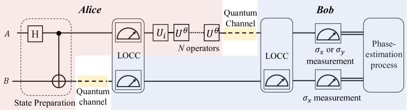
In this section, we describe the proposed quantum integrated sensing and communication protocol. The protocol involves three parties: the legitimate communication counterparts, Alice (the sender) and Bob (the receiver), along with the potential eavesdropper, Eve. We consider a scenario where Alice holds a collection of conditional payload messages that she intends to transmit to Bob, meanwhile Bob aims to conduct remote measurements at Alice’s location without compromising sensitive information to Eve. To achieve this goal, they harness the entangled photons detailed in Eq. (1) as quantum state resources for implementing the protocol. As depicted in Fig 3, the QISAC protocol consists of the following six steps.
Prior to the communication, Alice and Bob agree that the states corresponds to a specific mapping of bit 0, while the states corresponds to a specific mapping of bit 1.
Step 1, states preparation and distribution. Alice generates EPR pairs as the initial probe states, denoted by . Here, the subscript represents the index of EPR pairs in the sequence, while A and B denote the photon and its entangled partner in the EPR pairs respectively. Alice divides the initial EPR pairs into two partner photon sequences, referred to as sequence and sequence . She keeps for herself and sends to Bob via the quantum channel. This step completes the initial distribution of entangled pairs.
Step 2, first eavesdropping detection. After Bob receives the photon sequence , Alice and Bob follow these steps to detect eavesdropping: (i) Bob randomly selects partner photons from sequence with a probability of and measures the selected photons randomly on the , , or basis, (ii) Bob informs Alice about the positions and measurement bases of the selected photons and additionally shares the measurement outcomes with her through a classical authenticated channel, (iii) Alice measures the corresponding EPR partner photons in , using the same measurement bases chosen by Bob, and then compares the measurement results. Alice then obtains the complete opposite results compared to Bob, provided that no eavesdropper contaminates the quantum channel. If the error rate is below the tolerance threshold, Alice and Bob conclude that no eavesdropper was present during the first transmission and proceed to the next step. Otherwise, they terminate the protocol due to the presence of eavesdroppers.
Step 3, encoding. In sequence , the remaining photons serve to carry confidential messages and the parameter to be transmitted. Alice first encodes the plaintext by applying
| (11) |
or
| (12) |
where and maps the bit and on to quantum state, respectively. Then she applies identical unitary operators to parameterize the encoded states, that is,
| (13) |
where is the parameter to be estimated. This operation transforms the encoded state into
| (14) |
and
| (15) |
During the encoding process, Alice applies an encoding trick within the sequence to guard against second eavesdropping. She randomly selects some photons from sequence with a probability of as samples to undergo one of the four unitary operators described by Eq. (2) in a disorderly manner. Importantly, these photons carry no valuable information mapped onto them but random numbers. Alice keeps the positions of sampling photons secret until confirming that Bob has received the sequence . Consequently, the ratio of photons carrying the confidential payload information is within the initial pairs, while the remaining ratio of of pairs serves for eavesdropping detection. We will discuss the trade-off related to the choice of under finite resource constraint in Sec. V.2.
Step 4, transmission and second eavesdropping detection. Alice sends the encoded EPR partner photon sequence to Bob via the quantum channel. Upon receiving the photon sequence, Bob is informed of the positions of the samples and the specific unitary operators applied to them. To ensure communication security, Bob performs Bell-state measurement on these photons and estimates the QBER. If the QBER of the checking pairs is reasonably low, Alice and Bob can trust the process and proceed to decode plaintext and estimate . Otherwise, they will abort and return to step 1.
Interestingly, Eve can perturb the qubits using a man-in-the-middle attack during the second transmission but cannot steal the payload messages. This limitation arises because one cannot read information from a single particle of an EPR pair alone, resulting in the maximum mixed state for an eavesdropper. Furthermore, any perturbations introduced by Eve can be detected based on the second estimated QBER.
The following steps 5 and 6 involve reading out the confidential messages and estimating the parameter .
Step 5, measurement. Bob measures each encoded EPR pairs on two measuring bases. He randomly chooses to perform the observable or with probabilities and respectively, where
| (16) |
and
| (17) |
Obviously, corresponds to the operator for Bell-state measurement.
Step 6, the parameter estimation process. After measurement, Bob decodes the information bit and estimates the parameter using the raw measurement data. The operators and each have four eigenvectors, corresponding to four detectors. As illustrated in Table 1, we calculate the probability distribution for different responses with the two observables, where
| (18) | ||||
are the eigenvectors of , and
| (19) | ||||
are the eigenvectors of .
| Eigenvectors | ||||||||
|---|---|---|---|---|---|---|---|---|
| Eigenvalues | -1 | 1 | 1 | -1 | -1 | 1 | 1 | -1 |
| 0 | 0 | 0 | 0 | |||||
| 0 | 0 | 0 | 0 | |||||
Explicitly, this means that when detector 3 or 4 of and detector 3 or 4 of respond, it corresponds to the quantum state , representing bit 0. Conversely, when detector 1 or 2 of and detector 1 or 2 of respond, it corresponds to the quantum state , denoting bit 1. By analyzing the distribution of detector responses, we can calculate the expected values of the two observables and estimate the phase value. The expected values of and are
| (20) | ||||
where
| (21) |
refers to the density matrix of mixed states received by Bob. The experimental expected value is obtained by classical calculation of measurement datas, with the formula , where and are the eigenvalues and response ratios of the -th detector. Then, Bob obtains an estimate from Eq. (20).
For each selected value of , Bob theoretically calculates and obtains the same estimation value from two operators. However, the dependencies of probabilities are complicated for the actual shared state used in experiment, even though the fidelity between the shared state is greater than 0.99 [27]. To solve the problem of fluctuating values obtained by distinct observables, Bob separately calculates the expected values of two operators. Then he estimates the parameter by two expected values, specifically and . The parameter estimate is then taken as the average of and , given by
| (22) |
After repeating the estimation measurement times, we can evaluate in error-propagation formula, Eq. (10), using the expectations and variances of two observables. The variances of two observables are
| (23) | ||||
Hence the variance and according to Eq. (10) are
| (24) | |||
By using the error-propagation theory, the error on , namely the variance can be obtained easily by
| (25) |
To minimize the variance, the and need to be performed with equal probability, hence we arrives
| (26) |
that is, Bob performs the observables and to measure the encoded EPR pairs randomly with 50% probability. The variance from error-propogation theory becomes
| (27) |
The quantum Fisher information defined in Eq. (7) can be expressed by [34]
| (28) | ||||
where the spectral decomposition of the density matrix is given by . Furthermore, is the dimension of the support set of . From this equation, one can find that the quantum Fisher information for a non-full rank density matrix is determined by its support. By plugging our system from Eq. (21) into the above equation, we obtain that the QFI is
| (29) |
and the corresponding quantum Cramér-Rao bound is
| (30) |
where the number of the measurement equals . By comparing Eq. 27 with the equation above, we find that the precision of parameter sensing can reach the quantum Cramér-Rao bound. This implies that our approach saturates the ultimate limit of unbiased estimate in QISAC protocol.
It is easy to observe that our scheme saturates the parameter estimation precision up to the Heisenberg-limit sensitivity. Recalling the QFI, which geometrically captures the rate of change of the evolved probe state under an infinitesimal variation of the parameter, it represents the maximum CFIs and signifies the optimal observable, denoted as . By substituting the probabilities in Eq. (6) with the values in Table 1, we obtain the CFIs for and , namely,
| (31) | ||||
This means that both and are optimal observables because the classical Fisher information saturates the quantum Fisher information.
In our QISAC protocol, Alice only needs to perform single-qubit measurements, eliminating the need for entangling operations. This aspect is crucial for reducing technological requirements. Moreover, our scheme is capable of conducting separable measurements, surpassing the standard quantum limit (), and achieving Heisenberg-limit sensitivity (). These features align with supports the conclusion demonstrated in [31]. Considering the operational complexity, our protocol offers practicality.
III.2 Further refinement of QISAC protocol
In terms of trading physical resources for time, achieving the same precision as the Heisenberg limit () is possible classically by repeatedly applying unitary maps times to the same probe state. This strategy is analogous to utilizing the NOON state [20], which takes the form of
| (32) |
The fundamental concept of enhancing precision through a multi-round strategy is intuitive. By employing passes, it effectively replaces with in both the probe states and the corresponding detection probabilities. Consequently, the CFI undergoes a quadratic enhancement, scaling by a factor of as depicted in Eq. (6). Similarly, the variance propagated from measurement errors also experiences an enhancement, scaling by a factor of as shown in Eq.10.
Due to the challenging preparation and susceptibility to decoherence of NOON states, we opt for the multi-round strategy, where the same photon in sequence undergoes identity unitary operators . Although this approach offers a straightforward and convenient means to improve measurement precision, it introduces a new challenge, as it narrows the estimable range of the parameter to . Expanding the parameter range to is the problem we need to address.
Various approaches exist to address this issue [35]. Alice could declare the range within which the transmitted parameter lies, but this would also narrow the range of parameter for Eve. Instead, we employ multiple passes of the operation with different . Specifically, a small fraction of photons in sequence are randomly selected to undergo only once, while the remaining photons undergo -operation times. Once both parties confirm the security of communication, Alice informs Bob which photons she has selected to pass through once. This allows Bob to estimate the parameter value based on the intersection of the two sets of passes. Notably, Fisher information is additive, i.e., , where represents the Fisher information of the -th subsystem. Therefore, the Fisher information becomes , implying that the smaller is, the closer the estimation precision is to . Here, we set , meaning that 10% of the photons in sequence pass once, while 90% of photons pass -operation times. So the quantum Cramér-Rao bound approaches the Heisenberg limit, denoted as
| (33) |
To illustrate this method more intuitively, we utilize the likelihood function curve of system . Based on the non-zero outcomes with different probabilities in Table 1, we derive the likelihood function of is
| (34) | ||||
where , , , and represent the photon numbers corresponding to their respective probabilities. Therefore, the likelihood function is given by , where we set .
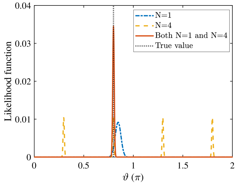
In Fig.4, we illustrate the effect of combining single-pass and four-pass operations. We simulate and plot three likelihood function curves using the same 140 EPR pairs, each normalized. The single-pass method produces a relatively broad likelihood function around the true value of , while the four-pass method yields narrower peaks but with a fourfold multiplicity, making it difficult to identify the true value. By combining single-pass and four-pass methods with the same quantity of qubits, we obtain a narrow peak at the correct value of . Although the combination method results in a relatively broad peak compared to the four-pass method, it indicates a limited increase in variance. Therefore, this approach effectively ensures estimation accuracy while also approximately approaching the Heisenberg limit.
IV Security analysis
The security of our QISAC protocol relies on two crucial assumptions. We assume that the shared Bell states are independent and identically distributed (i.i.d.), and Eve performs the same attack every time. Besides, authentication between Alice and Bob is assumed to be guaranteed. With these two assumptions in place, Alice and Bob can resist against Eve’s man-in-the-middle attack. In this scenario, Eve can entangle her auxiliary system with system by applying , after which she sends system to Bob. According to the quantum De Finetti theorem [36], the joint state of systems and asymptotically resembles a direct product of i.i.d. subsystems. Thus, it is sufficient to analyze an individual subsystem separately. To assess the security of the protocol, we divide it into two aspects: the security of information bit and the security of parameter estimation, employing Wyner’s wiretap channel theory [37] and asymmetric Fisher information gain respectively.
IV.1 Securiy of information bit
The extent of eavesdropping can be assessed by examining the QBER. In this section, we aim to determine the secrecy capacity bound for our scheme. According to the Wyner’s wiretap channel theory [37], there exists a coding method that facilitates secure and reliable information transmission at a rate below the secrecy capacity, providing the secrecy capacity is positive. The secrecy capacity of secure communication for our scheme is
| (35) |
where and represent the channel capacities of the main and wiretap channels, respectively. To evaluate the wiretap channel capacity, we will examine the specific process of eavesdropping. Without loss of generality, we can define the attack as an identical and individual unitary transformation applied to the emitting state by Alice in the channel, representing a collective attack scenario. The mathematical description of an EPR pair’s state after the first transmission is
| (36) |
We can eliminate all the nondiagonal elements of in Bell basis [38] based on introducing operators that two users both apply the same transformation randomly from , and has the simple form , where . The parameter is controlled by the malicious third party, Eve. Thus, the purification of state is
| (37) |
where is the Bell state of system and is the set of orthogonal states of system . The parameter is determined by the QBER , and for the , and bases in first transmission respectively, that is, , and . Tracing out system from system , we can get system is
| (38) |
where
| (39) | ||||
After the first transmission, Alice encodes system through performing and . So the encoded states are
| (40) | |||
| (41) |
where represents a 4-dimensional identity matrix. If the quantum channel is modeled as a depolarizing channel , the QBERs in the first eavesdropping check are . We assume that each qubit has the same distribution, and the partner photons transmit through a depolarizing channel. Thus, we apply the Holevo bound to obtain the mutual information between Alice and Eve. The upper bound on the information that Eve can steal is
| (42) | ||||
where is QBER in first transmission. Here, we denote the binary Shannon entropy by .
The capacity of the main channel can be described based on the two QBERs in both transmissions. We reasonably assume that our two-qubit encoding scheme is a two-fold tensor product of a single depolarizing channel. In other words, after both particles of an EPR pair pass through the channel, the probability of the depolarizing channel becomes . Since Bob measures the EPR pairs in two observables separately, we can compute the mutual information between Alice and Bob in two measurement bases, which are
| (43) |
We find that the two mutual informations performing and are equal. Thus, the lower bound of the secrecy capacity is
| (44) |
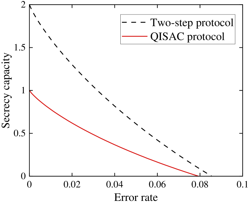
In the simplification scenario where , the tight estimation of the secrecy capacity for modified two-step QSDC in the depolarizing channel is , as shown by Eq. (3). We plot and compare the secrecy capacity versus the QBER between our scheme and the modified two-step QSDC protocol in Fig. 5. The results shows that the entire curve of our QISAC scheme lies below that of the two-step QSDC protocol. At low errorrates, the latter’s capacity is twice that of our scheme, but it rapidly diminishes to zero as the error rate increases. To be more specific, the QBER threshold for our QISAC scheme is 7.9%, while the threshold of the two-step protocol is 8.6%. The QISAC protocol maintains secure until the QBER exceeds the computed threshold. However, it is less resilient to channel noise due to our choice of encoding, which carries one-bit information on a single EPR pair instead of dense coding. We intentionally sacrifice one bit position to encode the phase parameter on it, enabling integrated quantum communication and quantum sensing using these entangled EPR pairs.
Note that the double CNOT attack [29] enables the distinction between and in the transmission of confidential information via Bell states. Next, we will demonstrate the robustness of the proposed QISAC protocol against such attacks. In the first transmission, Alice generates EPR pairs in and sends to Bob. When the particles in passes through the quantum channel, Eve applies the first CNOT gate on the qubit as the control bit, and her own qubit as the target qubit. After that, the system becomes
| (45) |
Tracing out system from , we can get system is
| (46) |
If Alice and Bob both measure in basis, the probabilities of outcomes or are
| (47) |
Without the double CNOT attack from Eve, Alice and Bob get deterministic opposite results,
| (48) |
In other word, the double CNOT attack would result in a 50% QBER when measuring in the -basis. Similarly, when both Alice and Bob measure in the -basis, they also encounter a 50% QBER. However, measuring in the -basis does not introduce errors during the eavesdropping check.
In the depolarizing channel, the QBERs , and should be approximately equal. Consequently, once two legitimate users observe that and deviate significantly from , they will terminate the transmission and revert to step 1. This approach effectively counters the double CNOT attack launched by malicious eavesdroppers.
IV.2 Security of phase estimaiton
As demonstrated in the quantum remote sensing protocol [27], the security level of phase estimation is characterized by the asymmetric Fisher information gain. To assess how much Fisher information Bob acquires in the protocol under depolarizing circumstances, we calculate a new set of probabilities for two observables, where the non-zero value becomes and becomes , the other probabilities are still . Substituting the probabilities of Eq. (6) with new datas, we obtain
| (49) | |||
| (50) |
Clearly, the level of Fisher information can be assessed via the QBER. Since Fisher information is additive, the Fisher information Bob gains satisfies
| (51) |
To quantify the Fisher information acquired by the eavesdropper, we assume that Eve possesses formidable capabilities, constrained only by the principles of quantum physics. Since all information available to Eve originates from Alice, we substitute the mixed state density matrix from Eq. (40) and Eq. (41) into Eq. (7) to compute Eve’s quantum Fisher information, yielding
| (52) |
The Fisher information and versus the QBER are depicted in Fig. 6. The blue area between these two curves constitutes an asymmetric gain, that is, if the QBER falls within this area for our integrated scheme , we can reliably guarantee the security of parameter estimation, and the QBER threshold corresponding to the intersection is 8.3%.
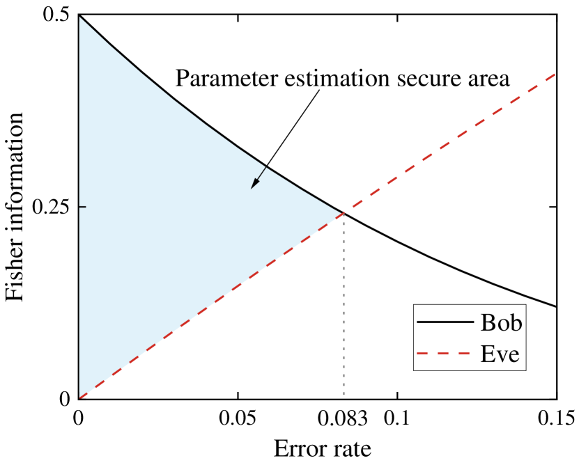
Combined the two thresholds, the security of this proposal is confirmed through a purely mathematical derivation of both quantum communication and quantum remote sensing aspects. As long as the QBER during transmission remains below 7.9%, our scheme remains secure.
V Performance analysis
V.1 Advantages of using two observables
Let us explore the advantages of performing two observables. Consider an experiment with measurements, where the number of results for each non-zero outcome with probabilities given in Table 1 is denoted as , where and the sum of is equal to . For ease of calculation, the value of in this section is 1 unless otherwise specified. Utilizing Eq. (5), which provides Bob’s likelihood function for , we arrives at
| (53) | ||||
The likelihood function of is and that of is , while is the product of and . Under the condition of utilizing 500 EPR pairs as probe states, we simulate the measurement process and plot the likelihood function curves for three different observable schemes, comparing them with the true value 0.8.
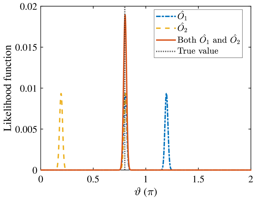
Table 1 reveals that the probabilities of non-zero measurement outcomes for and depend solely on and , respectively. Consequently, the estimation based on either observable alone can only cover the parameter range due to their symmetric likelihoods within the interval, as depicted in Fig. 7. This ambiguity is resolved by utilizing two sets of measurement bases orthogonal to each other on the Bloch sphere, allowing for estimation across the entire range.
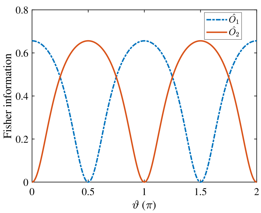
An additional reason for employing both observables lies in maintaining security within noisy quantum channel. While we have previously demonstrated that and are both optimal observables in ideal scenario in Sec. IV. But their optimality no longer holds in a noisy environment, and the CFIs have been previously derived and are given by Eq. (49) and Eq. (50). Obviously, these CFIs are functions of the unknown parameter , which fluctuate in value as changes. With a fixed value of 5%, we plot the change in CFI with respect to the parameter to be estimated in Fig. 8. Although implementing two observable variables is more complex than with one, the overall benefits significantly outweigh the drawbacks.
V.2 Limited resources
The available entanglement resources are limited in real-life implementation. We must consider the performance of the QISAC protocol in parameter estimation under the constraint of limited resources. In the asymptotic regime, using expected values to estimate the parameter yields an estimate very close to the true value, with minimal fluctuations introduced solely by inherent instrument errors. As depicted in Fig. 7, the likelihood function becomes an increasingly narrow normal distribution centered around the true value of . However, when dealing with limited data, we need to account for potential bias in the estimate of , which arises due to the constraints imposed by finite data availability.
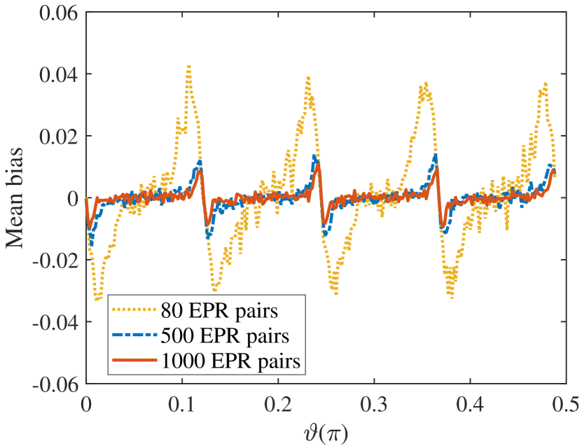
We simulate and plot the mean bias for different values with varying photon numbers in Fig. 9, where ranges from to . To mitigate systematic errors, we repeat each parameter estimation times, average the results, and findly compare them with the true value. Fig. 9 reveals that for most values, the bias remains smaller than the variance , where represents the number of measurements, corresponding to the number of EPR pairs in the legend. This observation the robustness of the QISAC protocol’s estimation method even under finite entanglement resources, rendering it a reliable approach. The improvement in accuracy does not increase linearly with the augmentation of entanglement resources. Initially, substantial gains are achieved, but as the entanglement resources expands, the accuracy improvement becomes progressively gradual. This behavior arises from inherent limitations in the method itself.
When the true value of aligns with an integer or half-integer multiple of , the estimated value of exhibits more significant bias, and this phenomenon becomes pronounced with fewer entangled photons. To optimize their estimation method, Alice and Bob can avoid this region by establishing a prior angle and using it to shift away from the problematic range.
Under the finite resource assumption, an intrinsic trade-off exists between achievable precision and security against the double CNOT attack and general man-in-the-middle attack. In the first checking round, each qubit intercepted and subjected to the CNOT gate by Eve randomly has a probability of introducing an error signal for Bob, provided that Bob measures the sampling qubits in either or basis. As previously mentioned, the legitimate parties can abandon the protocol if they detect Eve during the security check. The probability of selecting photons as eavesdropping-check samples is . Assume Eve intercepts and measures every qubit to obtain information, the probability of detecting Eve against the double CNOT attack is denoted by
| (54) |
where is the total numbers of qubits generated and distributed by Alice. In the case of the general man-in-the-middle attack, Eve intercepts and measures each qubit in , , or basis randomly, resulting in a error probability respectively for Bob. If the number of qubits intercepted by Eve is , the probability of detecting Eve against general man-in-the-middle attack is
| (55) |
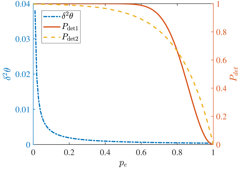
Fig. 10 provides a detailed illustration of the precision-security trade-off relationship. As the encoded ratio increases, more resources are allocated to the parameter estimation process, resulting in reduced variance of the estimate. However, this allocation comes at the cost of diminished security, as fewer resources remain for the security checking. When the value of is small, the solid curve representing resistance to the double CNOT attack exhibits a gradual descent rate, and remains around until the value reaches . At this point, the QISAC protocol demonstrates robust resistance to the double CNOT attack. Interestingly, as the value increases further, the curve experiences a sudden drop and intersects with , a dashed curve that provides defense against the general man-in-the-middle attack. When becomes large, the QISAC protocol exhibits better resistance to general man-in-the-middle attack than to double CNOT attack. Conventionally, we can optimize one aspect while considering the impact on the other, achieve a desired trade-off between security and precision.
V.3 Optimal Value of
In Sec. III, we employ a multi-round strategy to saturate the Heisenberg limit and refine the proposed QISAC protocol which allocate 10% of photons in sequence to pass through a single operation . Although the number of passes in the multi-round strategy is not necessarily linearly related to precision. Fig. 11 illustrates the optimal value of with 100, 400, 800 and 1200 EPR pairs. The mean bias, representing the average bias across values ranging from to , informs our choice of optimal resource allocation.
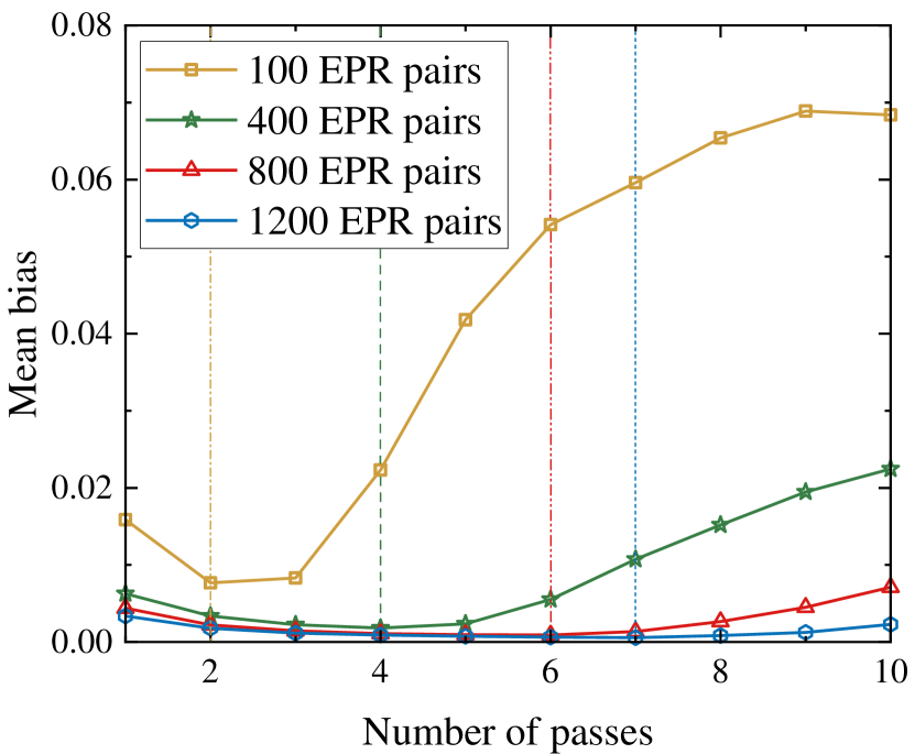
Initially, the mean bias decreases as the number of passes increases. However, if there are too many passes for the photons, the mean bias starts to increase again. The optimal value of tends to be smaller when the number of photon pairs is fewer. This phenomenon arises because the range of is divided into with the -pass method, resulting in a narrower accurate estimation range of as the number of passes increases. However, the combination of becomes increasingly challenging for determining the exact interval of , particularly evident with fewer EPR pairs, leading to larger fluctuations in estimates. Therefore, Alice and Bob can choose the appropriate value of according to their specific circumstances.
VI Conclusions and outlook
We propose a QISAC protocol, which enables distant communication parties to achieve secure and reliable quantum sensing alongside quantum-secured direct communication. By transmitting EPR pairs, the precision of QISAC’s remote sensing can approach the Heisenberg limit. In the presence of a depolarizing noisy quantum channel, we demonstrate that the secrecy capacity and asymmetric information gain ensure the security of the QISAC protocol from both informational transmission and sensing-parameter perspectives. Through the performance analysis model we provide, various adjustment strategies are proposed to optimize the performance of the protocol.
An intriguing direction is to experimentally demonstrate this protocol and gradually enhance its capabilities. In the future, the quantum internet will be established gradually [39]. By considering both communicating parties in the protocol as two nodes in the network, QISAC would further enrich the functionality of quantum Internet.
VII Acknowledgements
We acknowledge support by the National Natural Science Foundation of China (Grants No. 12205011 and 62131002), the Open Research Fund Program of the State Key Laboratory of Low-Dimensional Quantum Physics under Grant No. KF202205, Beijing Advanced Innovation Center for Future Chip (ICFC). We acknowledge the helpful discussions with Dr. Sean William Moore.
References
- [1] R. Horodecki, P. Horodecki, M. Horodecki, and K. Horodecki, “Quantum entanglement,” Reviews of Modern Physics, vol. 81, no. 2, p. 865, 2009.
- [2] A. K. Ekert, “Quantum cryptography based on Bell’s theorem,” Physical Review Letters, vol. 67, no. 6, p. 661, 1991.
- [3] M. Hillery, V. Bužek, and A. Berthiaume, “Quantum secret sharing,” Physical Review A, vol. 59, no. 3, p. 1829, 1999.
- [4] L. Xiao, G. L. Long, F.-G. Deng, and J.-W. Pan, “Efficient multiparty quantum-secret-sharing schemes,” Physical Review A, vol. 69, no. 5, p. 052307, 2004.
- [5] G.-L. Long and X.-S. Liu, “Theoretically efficient high-capacity quantum-key-distribution scheme,” Physical Review A, vol. 65, no. 3, p. 032302, 2002.
- [6] F.-G. Deng, G. L. Long, and X.-S. Liu, “Two-step quantum direct communication protocol using the einstein-podolsky-rosen pair block,” Physical Review A, vol. 68, no. 4, p. 042317, 2003.
- [7] J. H. Shapiro, D. M. Boroson, P. B. Dixon, M. E. Grein, and S. A. Hamilton, “Quantum low probability of intercept,” JOSA B, vol. 36, no. 3, pp. B41–B50, 2019.
- [8] D. Chandra, A. S. Cacciapuoti, M. Caleffi, and L. Hanzo, “Direct quantum communications in the presence of realistic noisy entanglement,” IEEE Transactions on Communications, vol. 70, no. 1, pp. 469–484, 2021.
- [9] J. Wu, G.-L. Long, and M. Hayashi, “Quantum secure direct communication with private dense coding using a general preshared quantum state,” Physical Review Applied, vol. 17, no. 6, p. 064011, 2022.
- [10] D. Pan, G.-L. Long, L. Yin, Y.-B. Sheng, D. Ruan, S. X. Ng, J. Lu, and L. Hanzo, “The evolution of quantum secure direct communication: On the road to the qinternet,” IEEE Communications Surveys & Tutorials, pp. 1–1, 2024.
- [11] J. Sternberg, J. Voisin, C. Roux, Y. Chassagneux, and M. I. Amanti, “Secure communication based on sensing of undetected photons,” arXiv preprint arXiv:2403.15557, 2024.
- [12] D. Pan, X.-T. Song, and G.-L. Long, “Free-space quantum secure direct communication: Basics, progress, and outlook,” Advanced Devices & Instrumentation, vol. 4, p. 0004, 2023.
- [13] Z. Cao, Y. Lu, G. Chai, H. Yu, K. Liang, and L. Wang, “Realization of quantum secure direct communication with continuous variable,” Research, vol. 6, p. 0193, 2023.
- [14] A. Patra, R. Gupta, T. Das, and A. S. De, “Dimensional advantage in secure information trading via the noisy dense coding protocol,” arXiv preprint arXiv:2310.20688, 2023.
- [15] B. Sephton, A. Vallés, I. Nape, M. A. Cox, F. Steinlechner, T. Konrad, J. P. Torres, F. S. Roux, and A. Forbes, “Quantum transport of high-dimensional spatial information with a nonlinear detector,” Nature communications, vol. 14, no. 1, p. 8243, 2023.
- [16] L. Zhou, Y.-B. Sheng, and G.-L. Long, “Device-independent quantum secure direct communication against collective attacks,” Science Bulletin, vol. 65, no. 1, pp. 12–20, 2020.
- [17] W. Zhang, D.-S. Ding, Y.-B. Sheng, L. Zhou, B.-S. Shi, and G.-C. Guo, “Quantum secure direct communication with quantum memory,” Physical Review Letters, vol. 118, no. 22, p. 220501, 2017.
- [18] F. Zhu, W. Zhang, Y. Sheng, and Y. Huang, “Experimental long-distance quantum secure direct communication,” Science Bulletin, vol. 62, no. 22, pp. 1519–1524, 2017.
- [19] Z. Qi, Y. Li, Y. Huang, J. Feng, Y. Zheng, and X. Chen, “A 15-user quantum secure direct communication network,” Light: Science & Applications, vol. 10, no. 1, p. 183, 2021.
- [20] V. Giovannetti, S. Lloyd, and L. Maccone, “Quantum metrology,” Physical Review letters, vol. 96, no. 1, p. 010401, 2006.
- [21] V. Giovannetti, S. Lloyd, and L. Maccone, “Advances in quantum metrology,” Nature photonics, vol. 5, no. 4, pp. 222–229, 2011.
- [22] G. Tóth and I. Apellaniz, “Quantum metrology from a quantum information science perspective,” Journal of Physics A: Mathematical and Theoretical, vol. 47, no. 42, p. 424006, 2014.
- [23] L. Pezze, A. Smerzi, M. K. Oberthaler, R. Schmied, and P. Treutlein, “Quantum metrology with nonclassical states of atomic ensembles,” Reviews of Modern Physics, vol. 90, no. 3, p. 035005, 2018.
- [24] S. W. Moore and J. A. Dunningham, “Secure quantum remote sensing without entanglement,” AVS Quantum Science, vol. 5, no. 1, 2023.
- [25] H. Zhang, G.-Q. Qin, X.-K. Song, and G.-L. Long, “Color-detuning-dynamics-based quantum sensing with dressed states driving,” Optics Express, vol. 29, no. 4, pp. 5358–5366, 2021.
- [26] J. W. Z. Lau, K. H. Lim, H. Shrotriya, and L. C. Kwek, “NISQ computing: where are we and where do we go?,” AAPPS bulletin, vol. 32, no. 1, p. 27, 2022.
- [27] P. Yin, Y. Takeuchi, W.-H. Zhang, Z.-Q. Yin, Y. Matsuzaki, X.-X. Peng, X.-Y. Xu, J.-S. Xu, J.-S. Tang, Z.-Q. Zhou, et al., “Experimental demonstration of secure quantum remote sensing,” Physical Review Applied, vol. 14, no. 1, p. 014065, 2020.
- [28] M. T. Rahim, A. Khan, U. Khalid, J. u. Rehman, H. Jung, and H. Shin, “Quantum secure metrology for network sensing-based applications,” Scientific Reports, vol. 13, no. 1, p. 11630, 2023.
- [29] A. Fahmi and M. Golshani, “Comment on “quantum key distribution in the holevo limit”,” Physical review letters, vol. 100, no. 1, p. 018901, 2008.
- [30] J. Wu, Z. Lin, L. Yin, and G.-L. Long, “Security of quantum secure direct communication based on wyner’s wiretap channel theory,” Quantum Engineering, vol. 1, no. 4, p. e26, 2019.
- [31] W. Zhong, X. M. Lu, X. X. Jing, and X. Wang, “Optimal condition for measurement observable via error-propagation,” Journal of Physics A: Mathematical and Theoretical, vol. 47, no. 38, p. 385304, 2014.
- [32] S. L. Braunstein, C. M. Caves, and G. J. Milburn, “Generalized uncertainty relations: theory, examples, and lorentz invariance,” annals of physics, vol. 247, no. 1, pp. 135–173, 1996.
- [33] C. W. Helstrom, “Quantum detection and estimation theory,” Journal of Statistical Physics, vol. 1, pp. 231–252, 1969.
- [34] J. Liu, X.-X. Jing, W. Zhong, and X.-G. Wang, “Quantum fisher information for density matrices with arbitrary ranks,” Communications in Theoretical Physics, vol. 61, no. 1, p. 45, 2014.
- [35] D. W. Berry, B. L. Higgins, S. D. Bartlett, M. W. Mitchell, G. J. Pryde, and H. M. Wiseman, “How to perform the most accurate possible phase measurements,” Physical Review A, vol. 80, no. 5, p. 052114, 2009.
- [36] R. Renner, “Symmetry of large physical systems implies independence of subsystems,” Nature Physics, vol. 3, no. 9, pp. 645–649, 2007.
- [37] A. D. Wyner, “The wire-tap channel,” Bell system technical journal, vol. 54, no. 8, pp. 1355–1387, 1975.
- [38] B. Kraus, N. Gisin, and R. Renner, “Lower and upper bounds on the secret-key rate for quantum key distribution protocols using one-way classical communication,” Physical Review Letters, vol. 95, no. 8, p. 080501, 2005.
- [39] S. Wehner, D. Elkouss, and R. Hanson, “Quantum internet: A vision for the road ahead,” Science, vol. 362, no. 6412, p. eaam9288, 2018.