Estimating Breakpoints between Climate States in Paleoclimate Data

This study presents a statistical approach for identifying transitions between climate states, referred to as breakpoints, using well-established econometric tools. We analyse a 67.1 million year record of the oxygen isotope ratio $\delta^{18}$O derived from benthic foraminifera. The dataset is presented in Westerhold et al., (2020), where the authors use recurrence analysis to identify six climate states. We consider several model specifications. Fixing the number of breakpoints to five, the resulting breakpoint estimates closely align with those identified by Westerhold et al., (2020) across various data binning frequencies and model specifications. Treating the number of breakpoints as a parameter to be estimated results in statistical justification for more than five breakpoints in the time series. Our approach offers the advantage of constructing confidence intervals for the breakpoints, and it allows testing for the number of breakpoints present in the time series.

1 Introduction

Beneath the ocean floor, a vertical record of Earth’s climate history is preserved in the shells of benthic foraminifera. By drilling cores of these sediments, one can investigate this history dating back millions of years. A widely used paleoclimate variable is $\delta^{18}$O, which acts as a temperature proxy. Westerhold et al., (2020) present a data set spanning from 67.1 million years ago (Ma) to the present time, covering the Cenozoic Era. The authors use recurrence analysis to identify six climate states: Warmhouse I, Hothouse, Warmhouse II, Coolhouse I, Coolhouse II, and Icehouse, and thus five transitions. The climate states in the Cenozoic Era range from very warm climates to the glaciation of Earth’s polar regions (Zachos et al., , 2001). The climatic transitions contain important information about variations in Earth’s climate system, and understanding them may help forecast future transitions; see Tierney et al., (2020) for a review. Our study presents a statistical approach for identifying transitions between climate states, referred to as breakpoints, using well-established econometric time-domain tools as proposed by Bai and Perron, (1998, 2003). Our approach offers the advantages of constructing confidence intervals for the breakpoints, providing a measure of estimation uncertainty, and testing for the number of breakpoints in the time series.

We adopt the estimation methodology of Bai and Perron, (1998, 2003) which necessitates a constant observation frequency and a predetermined model specification. To obtain a constant observation frequency, we use the method of mean binning which entails dividing the data in intervals of fixed length and calculating the mean in each bin. We explore three model specifications and implement these using the R-package by Nguyen et al., (2023). The first model is a state-dependent mean model, which is equivalent to a model with an abrupt break in the mean of $\delta^{18}$O for each climate state. The second model generalises this by including a state-independent autoregressive term, which can be interpreted as making the transitions between states more gradual. The final model extends the second model by letting the autoregressive term be state-dependent as well, allowing for state-specific autoregressive dynamics. All models incorporate an error term with state-dependent variance. Given that the time series appears state-wise non-stationary (meaning that the mean and variance of the time series vary over time) across most of the record, we conduct a simulation study to demonstrate the applicability of the approach by Bai and Perron, (1998, 2003) in this non-stationary setting.

Fixing the number of breakpoints to five, the resulting breakpoint estimates align closely with those identified by Westerhold et al., (2020) across various binning frequencies and model specifications. This demonstrates the robustness of the approach and corroborates the dating of the climate states of Westerhold et al., (2020) with statistical analysis in the time domain. However, when we also estimate the number of breakpoints in the time series using information criteria, we find strong statistical evidence for the presence of more breakpoints.

Research related to the climate states during the Cenozoic Era has intensified due to improved data availability. Key contributions include Westerhold et al., (2020) for oxygen and carbon isotope records and the composite paleo-CO₂ record by the CenCO2PIP Consortium, (2023). Notably, Boettner et al., (2021) aim to identify early warning signals prior to climatic events in the Cenozoic Era using the Westerhold et al., (2020) dataset. They split the dataset up into multiple sections and analyse them individually using the breakpoints by Westerhold et al., (2020). One advantage of our approach is that the full time frame of the dataset can be considered in a single model and that the breakpoints between climate states can be estimated within the model framework. Rousseau et al., (2023) apply Kolmogorov-Smirnov tests in addition to recurrence analysis to find breakpoints similar to those by Westerhold et al., (2020). Furthermore, Reikard, (2021) presents a forecasting study using parts of the dataset.

The methodology used by Westerhold et al., (2020) to identify breakpoints is based on recurrence analysis and is outlined in Marwan et al., (2007). Although this method is well-established in the paleoclimate literature, it does not provide measures of uncertainty. Marwan et al., (2021) reviews methods for identifying and characterising breakpoints in paleoclimate time series, and Marwan, (2023) discusses challenges in the use of recurrence analysis. Additional research includes Ruggieri, (2013), who introduces a Bayesian algorithm for breakpoint detection. Goswami et al., (2018) propose a breakpoint detection method using a probability density function sequence representation of the time series. Furthermore, Livina et al., (2010) develop a statistical method for detecting the number of states in a geophysical time series. Our approach contributes to the existing breakpoint detection methods in paleoclimate research by offering a simple yet comprehensive framework. It enables the estimation of multiple breakpoints along with confidence intervals and provides procedures to estimate the number of breakpoints, enhancing the analysis of paleoclimate time series.

The remainder of the paper is structured as follows: In Section 2, we present the $\delta^{18}$O dataset and climate states by Westerhold et al., (2020). Then, in Section 3, the methodology applied in this project is outlined. In Section 4, we conduct the analysis and discuss the results. Section 5 concludes. The performance of the methodology under state-wise non-stationarity is investigated in Appendix A.

2 Data

The paleoclimate variable $\delta^{18}$O measures the ratio of ¹⁸O to ¹⁶O relative to a standard sample. The weight difference between the oxygen isotopes leads to an inverse relationship between ocean temperatures and the $\delta^{18}$O measurements from ocean sediment cores containing benthic foraminifera; see for instance, Epstein et al., (1951) and Shackleton, (1967).

In this paper, we employ the dataset provided in the study by Westerhold et al., (2020), which compiles measurements of oxygen and carbon isotope ratios from benthic foraminifera across 34 different studies and 14 ocean drilling locations into a single data file. Our study focuses on the $\delta^{18}$O record, specifically the correlation-corrected observations of $\delta^{18}$O (column L “benthic d18O VPDB Corr”) from the data file. Westerhold et al., (2020) provide an estimated chronology of the data, which has accuracy ranging from $\pm 100$ thousand years (kyr) in the older part of the sample period to $\pm 10$ kyr in the younger part. We ignore the uncertainty of the time stamps in this study. The data covers the period 67.10113 Ma to 0.000564 Ma, and we order the observations from oldest to most recent. We remove the 74 missing values in the record, leaving us with 24,259 data points.

Westerhold et al., (2020) have identified six climate states using recurrence analysis by Marwan et al., (2007). The six climate states are Warmhouse I (66-56 Ma), Hothouse (56-47 Ma), Warmhouse II (47-34 Ma), Coolhouse I (34-13.9 Ma), Coolhouse II (13.9-3.3 Ma), and Icehouse (3.3 Ma to present). The top panel of Figure 1 shows the $\delta^{18}$O data along with the breakpoints between the climate states, as identified by Westerhold et al., (2020). Appendix C.1 shows summary statistics of the dataset for the full sample length and for each climate state.

The $\delta^{18}$O data presents unique challenges due to its coarse nature and intermittent gaps. To visualise the irregular time stamps of the $\delta^{18}$O data, the time between data points over time is shown in the bottom panel of Figure 1. This shows that the time series is relatively sparse in the older part of the record and relatively dense in the younger part. The mean time between two adjacent data points is approximately 2.8 kyr, and the longest gap between data points is approximately 115.4 kyr. There are 533 occurrences of gaps between two data points lasting longer than 10 kyr. Moreover, there are 591 instances of multiple observations at the same time stamp, with up to four simultaneous observations.

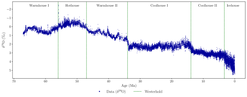
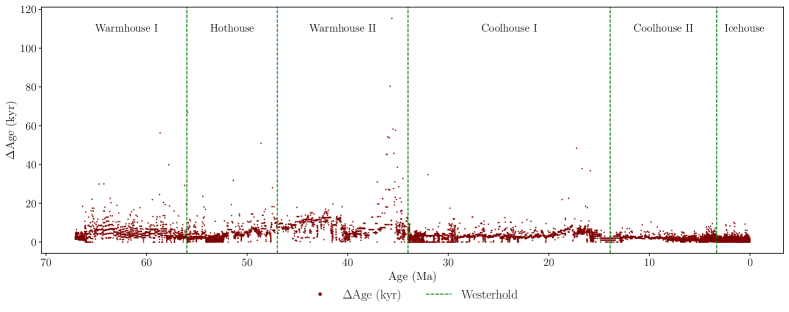
Figure 1: Top panel: $\delta^{18}$O data. Bottom panel: The time between data points of $\delta^{18}$O data measured in kyr. The vertical dashed lines denoting transitions between the climate states by Westerhold et al., (2020). The horizontal axis represents time, measured in millions of years before present.

3 Methodology

In this section, we present and discuss the methodology developed by Bai and Perron, (1998, 2003) for estimating breakpoints in linear regression models. Section 3.1 provides an outline of the framework for detecting multiple structural changes in linear regression coefficients and for constructing confidence intervals for the breakpoints. Section 3.2 discusses the model specifications employed in this study for breakpoint estimation. Section 3.3 presents methods for testing for the presence of structural breaks and estimating the number of breakpoints.

3.1 General framework

This method is based on minimising the sum of squared residuals while treating the breakpoints as unknown parameters to be estimated (Bai and Perron, , 1998, 2003). Consider a linear regression framework for the dependent variable $y_{t}$, for $t=1,\ldots T$, and with $m$ breakpoints, corresponding to $m+1$ distinct states in the sample, and with model equation

$$y_{t} =x_{t}^{\prime}\beta+z_{t}^{\prime}\delta_{j}+u_{t},\quad t=T_{j-1}+1,\ldots,T_{j}$$ (1)

with $j=1,\ldots,m+1$, the $m$ break dates are denoted by $\left(T_{1},\cdots,T_{m}\right)$ with the convention that $T_{0}=0$ and $T_{m+1}=T$ and $u_{t}$ is the disturbance term with mean zero and variance $\sigma_{j}$. The $(p\times 1)$-vector $x_{t}$ and the $(q\times 1)$-vector $z_{t}$ comprise two sets of covariate vectors, for which $\beta$ is the state-independent vector of coefficients and $\delta_{j}$ is the state-dependent vector of coefficients. Since only specific coefficients are subject to structural breaks, this model is referred to as a partial structural change model. Moreover, breaks in the variance of $u_{t}$ at the break dates $T_{1},\ldots,T_{m}$ can be considered. The parameters $\beta$ and $\delta_{j}$ are estimated alongside the breakpoints but are not of primary interest here.

For now, we will treat the number of breakpoints, $m$, as known and estimate the coefficients and the breakpoints using a sample of $T$ observations of $\left\{y_{t},x_{t},z_{t}\right\}$. The estimation method is based on the least-squares method for both the coefficients and the breakpoints. For each possible set of $m$ breakpoints $\left(T_{1},\ldots,T_{m}\right)$ denoted as $\left\{T_{j}\right\}$, we obtain estimates of $\beta$ and $\delta_{j}$ by minimising the the sum of squared residuals (SSR), that is

$$SSR= \sum_{j=1}^{m+1}\sum_{t=T_{j-1}+1}^{T_{j}}\left(y_{t}-x_{t}^{\prime}\beta-z_{t}^{\prime}\delta_{j}\right)^{2},$$ (2)

where $$\beta \delta_{j} j T_{j-1}+1 T_{j} \hat{\beta}\left(\left\{T_{j}\right\}\right) \hat{\delta}\left(\left\{T_{j}\right\}\right)$$ is common to all states while is specific for the state which is the period between and . The resulting estimated coefficients are denoted as and . These coefficients are then used to determine the SSR associated with each set of breakpoints,

$$SSR_{T}\left(T_{1},\cdots,T_{m}\right) \equiv\sum_{j=1}^{m+1}\sum_{t=T_{j-1}+1}^{T_{j}}\left(y_{t}-x_{t}^{\prime}\hat{\beta}\left(\left\{T_{j}\right\}\right)-z_{t}^{\prime}\hat{\delta}\left(\left\{T_{j}\right\}\right)\right)^{2}.$$ (3)

The estimated breakpoints are then given by

$$\left(\hat{T}_{1},\ldots,\hat{T}_{m}\right) =\underset{T_{1},\ldots,T_{m}}{\operatorname{argmin}}\;SSR_{T}\left(T_{1},\ldots,T_{m}\right).$$ (4)

The minimisation is conducted over all partitions $\left(T_{1},\ldots,T_{m}\right)$ such that $T_{i}-T_{i-1}\geq\dim(z_{t})$ to ensure that there are enough data points to estimate the parameters $\delta_{j}$ in each partition. This procedure leads to estimated parameters for the $m$ breakpoints, i.e., $\left\{\hat{T}_{j}\right\}$, $\hat{\beta}=\hat{\beta}\left(\left\{\hat{T}_{j}\right\}\right)$, and $\hat{\delta}=\hat{\delta}\left(\left\{\hat{T}_{j}\right\}\right)$. Since the breakpoints are discrete, this optimisation can be conducted using a grid search, which can be computationally heavy, especially for many breakpoints. Bai and Perron, (2003) introduce an efficient method for determining the global minimisers. For more details, we refer to Bai and Perron, (1998, 2003).

An essential advantage of this framework is that it allows for constructing confidence intervals for the breakpoints. This is not possible in the recurrence analysis approach implemented in Westerhold et al., (2020). The construction of confidence intervals is based on the asymptotic distribution of the break dates $\hat{T}_{j}$. A detailed account of the estimation strategy is outlined in Bai and Perron, (2003). The necessary convergence results for construction of the confidence intervals rely on a set of assumptions. For example, the construction of confidence intervals does not allow for covariates containing a stochastic trend. There are also two possible assumptions regarding the relationship between the errors and the covariates in $z_{t}$. If $z_{t}$ does not contain lagged dependent variables, then the residuals are allowed to have serial correlation and heteroscedasticity. Otherwise, if there are lagged dependent variables in $z_{t}$, then no serial correlation is permitted in the residuals.

3.2 Model specifications

In this section, we introduce the model specifications employed in this paper for estimating breakpoints. Three distinct specifications are considered, referred to as the ”Mean”, ”Fixed AR”, and ”AR” models. These are all special cases of the framework outlined in Equation (1). The Mean model, the simplest among them, is specified as follows,

$$y_{t} =c_{j}+u_{t},\quad\quad j=1,\ldots,m+1,$$ (5)

where $$c_{j} u_{t} x_{t}=0 z_{t}=1 \delta_{j}=c_{j} y_{t}$$ is the state-dependent intercept and is an error term. This model is equivalent to setting , , and in Equation (1). In this model, a breakpoint leads to an abrupt change in the mean of the dependent variable . The Fixed AR model extends the Mean model by incorporating an autoregressive term. We obtain the model

$$y_{t} =c_{j}+\varphi y_{t-1}+u_{t},\quad\quad j=1,\ldots,m+1,$$ (6)

where $$y_{t-1} \varphi c_{j} x_{t}=y_{t-1} \beta=\varphi z_{t}=1 \delta_{j}=c_{j}$$ is the dependent variable lagged by one period, and is the autoregressive coefficient which is constant over the whole sample. Here, the effect of a change in the coefficient would be more gradual since it depends on the autoregressive dynamics. The Fixed AR model is also a special case of Equation (1) by specifying , , , and .

The general AR specification also allows the autoregressive term to be state-dependent, resulting in the AR model,

$$y_{t} =c_{j}+\varphi_{j}y_{t-1}+u_{t},\quad\quad j=1,\ldots,m+1,$$ (7)

where the autoregressive coefficient $\varphi$ in Equation (6) is now state-dependent and is $\varphi_{j}$. This model is also obtained from (1) by setting $x_{t}=0$, $z_{t}=(1,y_{t-1})$, and $\delta_{j}=(c_{j},\varphi_{j})$. Here, both the intercept and the autoregressive coefficient are state-dependent. Thus, the three specifications are nested: the Mean model is a restricted Fixed AR model which in turn is a restricted AR model.

3.3 Determining the number of breakpoints

In this section, we address the issue of estimating the number of breaks $m$ in a time series. Bai and Perron, (1998) present both the option of utilising hypothesis tests and information criteria for this purpose. In this study, we utilise the double maximum test of the null hypothesis of no breakpoints versus the alternative of an unknown number of breakpoints up to an upper bound, $M$. This test can provide statistical evidence for the presence of breakpoints in a time series. To conduct the test, it is necessary to impose that the breakpoints are asymptotically different from each other. This is achieved by setting the minimum state length to be larger than a fraction of the sample size, denoted by $\varepsilon$. This so-called trimming parameter is defined as $\varepsilon=h/T$, where $h$ is the minimum length of a state. We refer to Bai and Perron, (1998, 2003) for critical values and further details.

We use information criteria to estimate the number of breakpoints. We consider the following three criteria: the Bayesian Information Criterion (BIC) by Yao, (1988) and the modified Schwarz Information Criterion (LWZ) by Liu et al., (1997), and the modified BIC (KT) by Kurozumi and Tuvaandorj, (2011). For all criteria, the estimated number of breakpoints is determined as the number of breakpoints which minimises the information criterion in question. Information criteria cannot take account of serial correlation in the error term. Bai and Perron, (2006) note that the BIC and LWZ criterion perform well in absence of serial correlation, but both of them lead to overestimation of the number of breakpoints in case of serial correlation in the error term.

4 Analysis and results

This section presents the results of our breakpoint analysis of the $\delta^{18}$O record presented by Westerhold et al., (2020). The irregular sampling is addressed by data binning in Section 4.1, which is required to conduct breakpoint estimation using the methodologies of Bai and Perron, (1998, 2003). Section 4.2 details the implementation of the models specified in Section 3.2. Section 4.3 addresses estimation of the number of breakpoints. Comparative analyses of the model specifications and the effects of varying binning frequencies are presented in Sections 4.4 and 4.5, respectively.

4.1 Constant data frequency

To handle the unevenly spaced data, we use a binning approach. This is common practice in time series analysis of paleoclimate data, see for instance Boettner et al., (2021) or Reikard, (2021). We divide the dataset into bins of fixed time intervals and compute the mean of the observations within each bin. We refer to this resulting data as the binned data. In the case of gaps in the binned data, we use the values immediately preceding and succeeding the section with missing data to perform linear interpolation. We consider six different bin sizes, namely 5, 10, 25, 50, 75, and 100 kyr. We provide summary statistics in Appendix C.1 for the full sample length and for each climate state by Westerhold et al., (2020) for all binning frequencies. To illustrate the binning approach, the top panel in Figure 2 shows the unaltered data along with the binned data at frequencies of 5 kyr and 100 kyr and the bottom panels zoom in on two sub-samples.

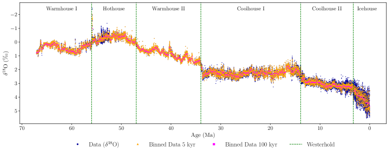
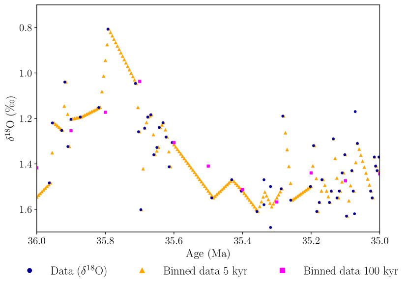
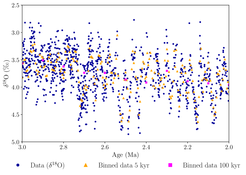
Figure 2: Top panel: The data and the 5 and 100 kyr binned data. Bottom left panel: Zoomed in on the period 36-35 Ma. Bottom right panel: Zoomed in on the period 3-2 Ma.

The top panel of Figure 2 shows that data binned at higher frequencies more closely follows the variations in the dataset, whereas data binned at lower frequencies tend to be smoother. Notably, the longest gap in the dataset lasts approximately 115 kyr and occurs between 36 Ma and 35 Ma. The bottom panels in Figure 2 zoom in on the periods 36 to 35 Ma (left) and 3 to 2 Ma (right). These plots illustrate that in case of large gaps (left), high binning frequency results in linear interpolation between observations. This effect does not occur for relatively short gaps (right). The binning approach offers a simple approach to handle the uneven frequency of the dataset. However, it can lead to data loss at lower binning frequencies and to the introduction of artificial data points resulting from linear interpolation at higher binning frequencies. Selecting inappropriate binning frequencies can alter the properties of the time series, potentially misrepresenting the dynamics of the original data.

4.2 Implementation

We consider three distinct model specifications, referred to as the Mean, Fixed AR, and AR models, specified in equations (5), (6), and (7), respectively. These models are implemented using the mbreaks R-package (Nguyen et al., , 2023) based on the methodologies of Bai and Perron, (1998, 2003). For all model specifications, we set the minimum length of a state, $h$, to 2.5 million years (Myr), facilitating the estimation of shorter climate states. Also, we let the variance of the error term, $\sigma^{2}_{j}$, be state-dependent.

The Mean model is implemented by setting $z_{t}=1$ and $x_{t}=0$ in Equation (1). The time series of $\delta^{18}$O is likely to be subject to both autocorrelation and heteroscedasticity in the errors. To address these issues, we use the autocorrelation and heteroscedasticity consistent (HAC) covariance matrix estimator with prewhitening in our implementation. The prewhitening procedure, proposed by Andrews and Monahan, (1992), entails applying a vector autoregressive of order one filter to $z_{t}\hat{u}_{t}$, where $\hat{u}_{t}$ denotes the residuals. The HAC covariance matrix estimator by Andrews, (1991) is then constructed based on the filtered series using the Quadratic Spectral kernel with the bandwidth selected by an AR$(1)$ approximation. This approach is also used for the Fixed AR model, which is implemented by setting $z_{t}=1$ and $x_{t}=y_{t-1}$ in Equation (1).

The AR model is implemented by setting $z_{t}=(1,y_{t-1})$ and $x_{t}=0$ in Equation (1). As outlined by Bai and Perron, (2003), no serial correlation is permitted in the errors in this type of model specification. The assumption of no serial correlation is strict in this case, since the incorporation of only one lag in the covariates is unlikely to resolve the issues related to serial correlation in the errors. Hence, we employ the HAC covariance matrix estimator with prewhitening in this implementation as well.

The theoretical framework by Bai and Perron, (1998, 2003) is developed for estimating and testing for multiple breakpoints in linear regression models, where the regressors are non-trending or state-wise stationary. However, the $\delta^{18}$O data appears non-stationary over most of the record, and we consider models with lagged dependent variables. As pointed out by Kejriwal et al., (2013), if the time series maintains its stationarity properties over the respective states, the methods developed for stationary data are still applicable for these cases. However, if the process alternates between stationary and unit root states, the theoretical properties of the methodology are unknown.

To investigate whether the time series is non-stationary, we apply the Augmented Dickey-Fuller (ADF) test (Dickey and Fuller, , 1979), with the null hypothesis of non-stationarity, and the KPSS test (Kwiatkowski et al., , 1992), with the null hypothesis of stationarity. When conducting the tests on the entire sample of 25 kyr binned data, the null hypothesis in the ADF test is not rejected, and the null hypothesis in the KPSS test is rejected, both at 1% significance levels. Examining the binned data for each of the climate states identified by Westerhold et al., (2020) separately, the null hypothesis in the KPSS test is rejected for each of them. However, in the ADF tests, the null hypothesis is rejected at 1% significance level for the Warmhouse II, Coolhouse I, and Icehouse states. Therefore, we need to examine whether the methodology of Bai and Perron, (1998, 2003) is applicable to data-generating processes that are state-wise non-stationary or alternating between stationary and non-stationary states.

Hence, we conduct a simulation study to examine potential challenges in conducting breakpoint estimation on these types of data-generating processes using the three model specifications. The study is conducted for both identically independently distributed (i.i.d.) error terms and serially correlated error terms in Appendices A.1 and A.2, respectively. The results indicate that the procedure works as intended also in the presence of non-stationarity. Moreover, the breakpoint estimation method appears robust to scenarios involving one stationary and one non-stationary state. In the case of serial correlation, the results are less conclusive, but if the states are sufficiently different, the methodology still appears effective. The study also reveals that the coverage rates of the estimated confidence intervals are generally adequate for the Mean and Fixed AR model specifications in cases of large breaks. Conversely, the confidence intervals for the AR model are too narrow in many of the data-generating processes considered.

4.3 Estimating the number of breakpoints

This section addresses the estimation of the number of breakpoints. First, we establish the presence of any breakpoints using the double maximum test for the 25 kyr binned data. The critical values for the double maximum test are available in the R-package mbreaks by Nguyen et al., (2023) for a trimming parameter $\varepsilon$ only down to 5% of the sample size and a maximum of 8 breakpoints. This is equivalent to 3.355 Myr as the minimum length of a state, which is slightly longer than the shortest climate state by Westerhold et al., (2020), the Icehouse state, lasting 3.3 Myr. The test statistics along with the critical values for each model specification are presented in Appendix C.2. The null hypothesis of no structural breaks is rejected at a 1% significance level for each of the models. We can therefore conclude that we do indeed find evidence for the presence of breaks in the time series.

To estimate the number of breakpoints, we use the information criteria discussed in Section 3.3. We find in the simulation study in Appendices A.1 and A.2 that the KT information criterion performs poorly, and hence, we exclude it from our analysis. We also find that the number of breakpoints estimated using the Mean model specification is generally overestimated when employing the information criteria. For the Fixed AR and AR models, the BIC and LWZ criteria typically perform well, especially in data-generating processes with a large break. With serial correlation in the error term, the BIC criteria tend to overestimate the number of breakpoints, whereas the LWZ criterion tends to perform well in the Fixed AR and AR model specifications.

We use the BIC and LWZ information criterion for each model specification and binning frequency, and set the minimum state length to $h=2.5$ Myr. Table 1 displays the estimated number of breakpoints, indicating a tendency towards a high number of breakpoints, increasing with the data frequency.

Bin size	Mean		Fixed AR		AR
	BIC	LWZ	BIC	LWZ	BIC	LWZ
5	19	17	17	7	15	5
10	17	17	14	7	14	3
25	17	14	12	6	8	3
50	17	14	10	0	7	0
75	17	14	6	0	5	0
100	17	12	6	0	5	0

Table 1: The number of breakpoints estimated using BIC and LWZ criterion for all models and binning frequencies considered. The minimum state length is set to $h=2.5$ Myr and the maximum number of breakpoints is 26.

The results in Table 1 show that the LWZ criterion suggests using a smaller number of breakpoints in the range from 3 to 7 in the higher frequency data in the Fixed AR and AR models. Furthermore, using binned data with too low or too high frequencies can affect the properties of the time series, as mentioned in Section 4.1. This analysis leads to statistical evidence for more than 5 breakpoints. We consider 1 to 15 breakpoints estimated using the 25 kyr binned data and the Fixed AR model in Appendix B.1. To maintain comparability with the findings of Westerhold et al., (2020), our subsequent analysis focuses on examining 3, 5, and 7 breakpoints.

4.4 Comparing the model specifications

In this Section, we compare the model specifications used to estimate breakpoints. We fix the number of breakpoints in the estimation process to $m\in\left\{3,5,7\right\}$ leading to 4, 6, and 8 states. Then, using the R-package mbreaks (Nguyen et al., , 2023), we estimate the breakpoints and corresponding 95% confidence intervals. In each estimation, we used a minimum state length of 2.5 Myr, allowing us to estimate relatively short climate states. The estimated breakpoints for all binning frequencies and model specifications are tabulated along with their 95% confidence intervals in the tables in Appendices C.3, C.4, and C.5 for 3, 5, and 7 breakpoints, respectively. As expected, the estimated confidence intervals around the breakpoints are often asymmetrical. Bai and Perron, (2003) advocate the use of asymmetric confidence intervals as these provide better coverage rates when the data is non-stationary.

To facilitate comparison of model specifications, we fix the frequency of the binned data to 25 kyr. Figure 3 shows the results and the $\delta^{18}$O data for 3, 5, and 7 breakpoints. Considering 3 breakpoints, the Mean and Fixed AR models both lead to estimated breakpoints at approximately 46.5 Ma, 34 Ma, and 13.9 Ma, aligning very well with the breakpoints identified by Westerhold et al., (2020). The AR model specification results in estimated breakpoints at 34 Ma, 13.9 Ma, and 2.6 Ma. The estimated breakpoints from the three model specifications align closely in the case of 5 breakpoints. The breakpoints from the 3 breakpoints case are preserved, and the confidence intervals for the Mean and the Fixed AR models are narrower. The estimated breakpoints align almost perfectly with those identified by Westerhold et al., (2020), and hence we can strongly corroborate their findings. When considering the 7 breakpoint case, the estimated breakpoints from the 5 breakpoints case are preserved. Both the Mean and Fixed AR models lead to additional estimated breakpoints around 39.7 Ma and 9.8 Ma, while the AR model leads to additional breakpoints at 53.3 Ma and 17.9 Ma. Further extending this analysis, Appendix B.1 shows the results of the estimation of 1 to 15 breakpoints in the Fixed AR model. The results show that the breakpoints identified by Westerhold et al., (2020) appear in all estimations that include 5 or more breakpoints.

As a robustness check, we re-estimate the model specifications for 5 breakpoints using the 25 kyr binned data reversed with respect to the time dimension, i.e., letting the time run backwards. The results are shown in Appendix B.2. We find that the results of the Mean and Fixed AR models are robust to reversing the time frame with almost unchanged estimated breakpoints. Conversely, the AR model leads to estimated breakpoints in the more recent part of the sample, resulting in breakpoints at 16.9 Ma and 9.7 Ma, which differ from those identified by Westerhold et al., (2020).

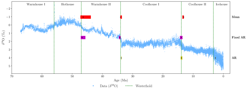
(a) 3 Breakpoints

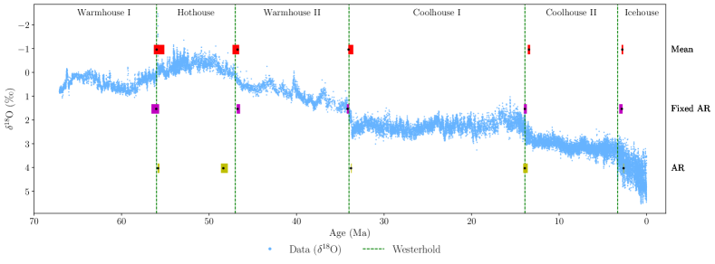
(b) 5 Breakpoints

(c) 7 Breakpoints

Figure 3: A comparison of estimated breakpoints using the Mean, Fixed AR, and AR model specifications on 25 kyr binned data for 3, 5, and 7 breakpoints. The black dots represent estimated breakpoints, while coloured shaded rectangles indicate 95% confidence intervals. The results overlay the $\delta^{18}$O data from Westerhold et al., (2020) and their climate states.

4.5 Comparing the binning frequency

This section examines the robustness of the estimated breakpoints across various frequencies of binned data. Initially, we fix the number of breakpoints to 5 and compare the estimated breakpoints using binned data of frequencies 5, 10, 25, 50, 75, and 100 kyr. The results are presented in Figure 4, with subfigures showing the results for the Mean, Fixed AR, and AR models.

For the Mean model in Figure 4a, it is evident that the estimated breakpoints generally remain at the same dates throughout as the binned data frequency decreases step-by-step from 5 kyr to 100 kyr. The width of the 95% confidence intervals increases as the frequency decreases, which can be attributed to the resultant decrease in the actual number of observations available for estimation at the lower frequencies. All the breakpoints align with those identified by Westerhold et al., (2020). A similar pattern of alignment is observed in the Fixed AR model, as depicted in Figure 4b.

Figure 4c presents the findings for the AR model, which exhibits more sensitivity to the frequency of the binned data. At higher frequencies, the breakpoints tend to appear in the more recent parts of the sample. At the 25 kyr frequency, the breakpoints correspond closely with those determined by Westerhold et al., (2020). However, as the frequency decreases further, the breakpoints are estimated to be in the older parts of the sample period.

In Appendix B.3, the analysis for 3 breakpoints is presented. For the Mean model, the confidence intervals become wide and even overlap at the lower frequencies, but the breakpoints themselves remain at approximately 46.3 Ma, 34 Ma, and 13.1 Ma. This is also the case for the Fixed AR model at frequencies 5, 10, and 25 kyr. However, at low frequencies, it becomes more unclear, and for the 100 kyr frequency, the confidence intervals of the first breakpoint reach outside the sample window. For the AR model, the estimated breakpoints for the higher frequency binned data coincide with the three final breakpoints by Westerhold et al., (2020), while for the lower frequency data, the estimated breakpoints appear in the older part of the sample.

For the seven-breakpoint estimation plotted in Appendix B.4, both the Mean and Fixed AR models generally corroborate the breakpoints identified by Westerhold et al., (2020), with additional breakpoints estimated at approximately 39.6 Ma and 10 Ma. In the AR model, most breakpoints coincide with those identified by Westerhold et al., (2020), with an exception around at the transition between Hothouse and Warmhouse II. Moreover, the additional breakpoints are estimated to be around 53 Ma and 17 Ma for the lower binning frequencies.

To summarise, the results of the Mean and Fixed AR models show robustness across different binning frequencies, while the AR model seems more sensitive towards varying the binning frequency. We therefore advocate to consider the Mean and Fixed AR models for the estimation of breakpoints in the $\delta^{18}$O time series presented by Westerhold et al., (2020). Furthermore, we advocate to use the frequencies 10 and 25 kyr as they present the most consistent outcomes.

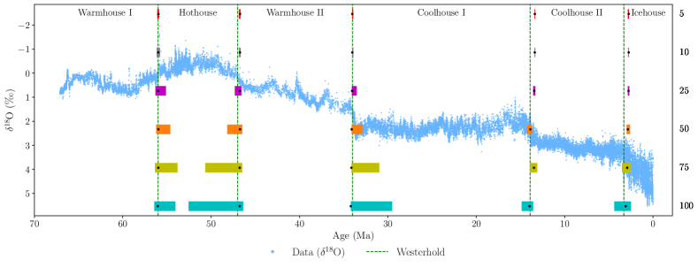
(a) Mean model

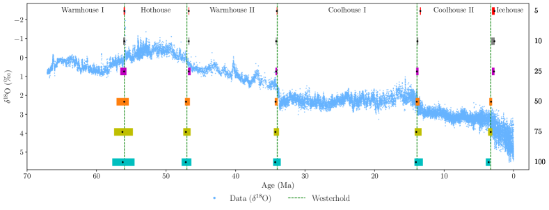
(b) Fixed AR model

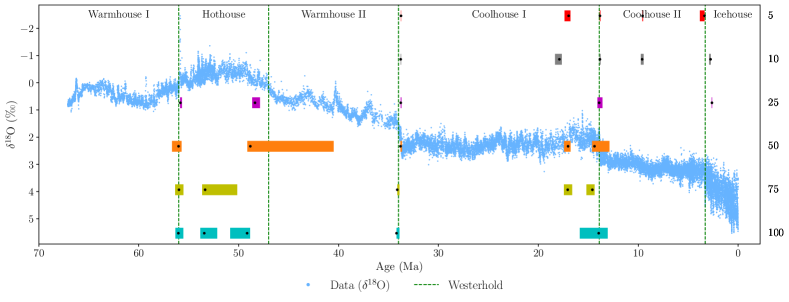
(c) AR model

Figure 4: A comparison of estimated breakpoints using binned data with frequencies of 5, 10, 25, 50, 75, and 100 kyr from top to bottom, fixing the number of breakpoints to 5 for each model specification. The black dots represent estimated breakpoints, while coloured shaded rectangles indicate 95% confidence intervals. The results overlay the $\delta^{18}$O data from Westerhold et al., (2020) and their climate states.

5 Conclusion

In this study, we propose a statistical approach to the estimation of breakpoints between climate states in the Cenozoic Era. We analyse the 67.1 million-year record of $\delta^{18}$O, which acts as a temperature proxy, presented by Westerhold et al., (2020). The authors of the study used recurrence analysis to identify five breakpoints, thus defining six climate states. We employ the well-established econometric tools developed by Bai and Perron, (1998, 2003). Within this framework, we consider three model specifications: a state-dependent mean model, an extended version with a state-independent autoregressive (AR) term, and a further extension with a state-dependent AR term. All models incorporate an error term with state-dependent variances. The first model corresponds to modelling an abrupt break in the mean of $\delta^{18}$O. The state-independent AR term in the second model allows for more gradual transitions between states. The final model introduces fully state-dependent autoregressive dynamics. Our approach allows for the construction of confidence intervals for the breakpoints, thereby providing a measure of estimation uncertainty. Furthermore, it allows for testing for the number of breakpoints in the time series.

The estimation of the models requires evenly time-stamped data, and therefore, we apply mean binning. We consider multiple binning frequencies: 5, 10, 25, 50, 75, and 100 kyr. We use the double maximum test to provide statistical evidence for at least one breakpoint in the time series. Then, we use information criteria to estimate the number of breakpoints. The results vary depending on the model specification and the binning frequency. Based on the results of our simulation study and using a binning frequency in the mid-range, we find statistical evidence for more than 5 breakpoints in the time series.

To maintain comparability with the findings of Westerhold et al., (2020), we focus mainly on 3, 5, and 7 breakpoints in our analysis. Fixing the number of breakpoints to 5, the resulting breakpoint estimates closely align with those identified by Westerhold et al., (2020) across various binning frequencies and model specifications, demonstrating the robustness of the approach. These results corroborate the dating of the transitions between climate states of Westerhold et al., (2020) with time series analysis. Considering 7 breakpoints, we find evidence that Warmhouse II and Coolhouse II can be split into two sub-periods. The two splits are also preserved when considering more than 7 breakpoints in the Fixed AR model as shown in Appendix B.1.

In a simulation study, we demonstrate that the methodology of Bai and Perron, (1998, 2003) is applicable in time series exhibiting state-wise non-stationarity and switching between stationarity and non-stationarity, even when incorporating serial correlation in the error term. This finding is notable, since the binned $\delta^{18}$O data exhibit non-stationarity in a state-wise manner. As a caveat, the estimated confidence intervals around the breakpoints are only adequate in the first two model specifications. Our examination of information criteria for estimating the number of breakpoints shows varying effectiveness across models in the simulation study. However, the model specification with a state-independent AR term shows promising results in both the accuracy of breakpoint estimation and the coverage rates of confidence intervals. Moreover, using the BIC and LWZ criterion in this model specification leads to high accuracy in estimating the number of breakpoints.

There are many directions in which our work could be extended in future, given the unresolved issues in statistical analysis of paleoclimate time series. It is evident that the binning method used in this study results in a considerable loss of information. In a follow-up project outlined in Bennedsen et al., (2024), we propose a continuous-time state-space framework for analysing the time series data by Westerhold et al., (2020), taking their breakpoints as given. This framework handles unevenly time-stamped data, multiple observations at the same time stamp, and measurement errors. Our future research will aim to incorporate the methodology by Bai and Perron, (1998, 2003) in a state-space framework, enabling utilisation of irregularly spaced and multivariate datasets when estimating breakpoints.

Appendix A Simulation study

A.1 Serially uncorrelated error term

In this appendix, we assess whether the methodology by Bai and Perron, (1998, 2003) can be used to accurately estimate the number and timing of breakpoints in a state-wise non-stationary time series. We conduct 1000 simulations for each data-generating process (DGP) each with a sample size of 500. All the DGPs considered have the following form,

$$y_{t} =c_{1}+\varphi_{1}y_{t-1}+\varepsilon_{t},\quad\varepsilon_{t}\overset{\textit{i.i.d.}}{\sim}\mathcal{N}\left(0,\sigma^{2}\right)\quad\text{ for }t\leq T/2$$

$$y_{t} =c_{2}+\varphi_{2}y_{t-1}+\varepsilon_{t},\quad\varepsilon_{t}\overset{\textit{i.i.d.}}{\sim}\mathcal{N}\left(0,\sigma^{2}\right)\quad\text{ for }t>T/2.$$ (8)

Hence, we consider a single breakpoint in the middle of the sample interval, namely at $t=250$. We examine eight DGPs, each specified and described in Table 2.

DGP	$\sigma$	$c_{1}$	$c_{2}$	$\varphi_{1}$	$\varphi_{2}$	Description
1	1	0.1	0.2	1	1	Small break in the drift term of a RW
2	1	0.1	1	1	1	Large break in the drift term of a RW
3	1	0.1	1	0.95	0.95	Large break in the intercept and a fixed AR-coefficient
4	1	0.1	1	0.95	1	Break in the intercept and small break in the AR-coefficient
5	1	0.1	1	0.5	1	Break in the intercept and large break in the AR-coefficient
6	1	1	1	1	1	RW with a drift without a breakpoint
7	0.5	0.1	1	1	1	Large break in the drift of a RW with low variance
8	1	0.1	1	0.5	0.5	Large break in the intercept and a low fixed AR-coefficient

Table 2: Data-generating processes for the simulation study and short descriptions.

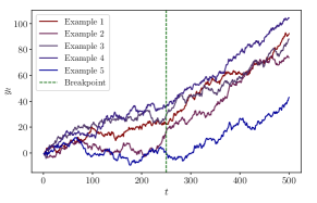
(a)

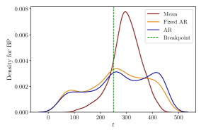
(b)

Figure 5: DGP 1: Left: Five process realisations. Right: The densities of the estimated breakpoints for each specification.

The DGPs range from random walk models with a break in the drift term to models with breaks in both the intercept and the AR coefficient. For comparison, we include a random walk without breakpoints as the sixth model. For each of the DGPs, we are interested in the performance of the methodology by Bai and Perron, (1998, 2003) to estimate the breakpoint and confidence intervals. The model specifications, i.e., the Mean, Fixed AR and AR models, from Section 3.2 are applied, and we use the implementation outlined in Section 4.2. We use the R-package mbreaks by Nguyen et al., (2023), and we impose a single breakpoint in the estimation. The left and right panels of figures 5 through 12 display realisations of the DGP and density plots of the estimated breakpoints for each of the models, respectively. The results are summarised in Table 3 which provides the mean of the estimated breakpoints, and medians of the lower and upper boundaries of the estimated 95% CIs are tabulated along with their coverage rates for each model and DGP.

In the first DGP, a random walk with a small drift term break, we observe that the mean of the estimated breakpoints is later than the true breakpoint in all model specifications. Additionally, the density plots exhibit asymmetry around the true breakpoint, which is expected given the low magnitude of the break in the drift term. In the second DGP with a larger drift term break, the estimated breakpoints exhibit a narrower and more bell-shaped density. The mean estimated breakpoints for the Fixed AR and AR models slightly precede the true breakpoint. However, the Mean model performs poorly with the mean of the estimated breakpoints far from the true breakpoint.

DGP	Mean				Fixed AR				AR
	BP est.	Lower	Upper	Coverage	BP est.	Lower	Upper	Coverage	BP est.	Lower	Upper	Coverage
1	301	174	655	57.1%	251	216	336	43.4%	290	240	316	22.7%
2	333	-386	332	95.4%	249	237	262	93%	249	236	256	77.2%
3	263	253	284	41.4%	256	239	260	89.9%	251	241	260	85.9%
4	340	-190	340	97.5%	249	239	260	95.8%	249	238	250	65.8%
5	340	-114	340	97.1%	250	239	258	97%	250	241	250	72.9%
6	249	-3325	3976	$\times$	253	142	371	$\times$	254	202	312	$\times$
7	333	-282	330	92%	249	246	253	97.8%	249	246	253	96%
8	249	237	264	95.1%	248	236	263	95.2%	248	236	263	94.5%

Table 3: Mean of the estimated breakpoints and medians of the lower and upper boundary of the estimated confidence intervals, along with the coverage rates for each model specification and DGP. DGP 6 is simulated without a breakpoint, so the coverage rate is irrelevant and indicated by $\times$.

In the third DGP, both the Fixed AR and AR models produce mean estimated breakpoints slightly later than the true breakpoint. The Mean model exhibits better performance in this DGP than in the second DGP. The fourth DGP has a break in the intercept and the AR-coefficient from 0.95 to 1, resulting in a state-wise non-stationary model. This change leads to breakpoint estimates very close to the true breakpoint, except in the Mean model. A similar outcome is observed in the fifth DGP, which features a larger increase in the AR-coefficient.

In the sixth DGP, which is defined without any breakpoints, the Mean model estimates breakpoints near the midpoint of the sample period, while the other two specifications yield inconclusive results. In the seventh DGP, the AR and Fixed AR models produce estimates close to the true breakpoint. However, the Mean model continues to produce breakpoint estimates far from the true value. Examining the eighth DGP, the three models perform almost equally well.

Overall, the Fixed AR and AR models tend to perform well in non-stationary scenarios, estimating breakpoints close to the true breakpoints. The methodology, however, appears to struggle with accurately estimating the true breakpoint in cases of minor changes between states and large error term variance. In contrast, the Mean model does not perform well in DGPs featuring gradual changes, aligning with theoretical expectations as detailed in Bai and Perron, (2003).

The coverage rate of a CI is the proportion of times the CI covers the true breakpoint at $t=250$. We find that the CIs of the Mean model are generally very wide and have varying coverage. In the Fixed AR and AR models, the CIs are typically narrower. The coverage rates are best in the DGPs with large differences between the states as seen in DGPs 4, 5, 7 and 8 using the Fixed AR model specification, which is in line with the findings of Bai and Perron, (2003). For the AR model, the coverage rates are only close to the desired 95% in the seventh and eighth DGP, indicating that the CIs are inadequate in most of the DGPs considered.

Table 4 shows the mean number of breakpoints estimated for each DGP and method, along with the proportion of correctly estimated breakpoints. The difficulty in accurately estimating gradual changes using the Mean model, is also evident when estimating the number of breakpoints. This model specification leads to overestimating the number of breakpoints in all DGPs considered except the DGP 8, where it performs well. The BIC criterion in the Fixed AR specification performs very well, with an estimated number of breakpoints equal to the true number in most simulations in DGP 2-8. The LWZ criterion performs almost equally well except in the third DGP, while the KT criterion vastly overestimates the number of breakpoints in DGP 1-7. In the AR model, the information criteria all perform well in DGPs 2-8 except for the third DGP where the LWZ criterion underestimates the number of breakpoints.

DGP	Mean			Fixed AR			AR
	BIC	LWZ	KT	BIC	LWZ	KT	BIC	LWZ	KT
1	3.0 (0%)	3.0 (0%)	3.0 (0%)	0.2 (15%)	0.0 (0%)	3.0 (0%)	0.1 (6%)	0.0 (0%)	0.0 (3%)
2	3.0 (0%)	3.0 (0%)	3.0 (0%)	1.0 (97%)	0.8 (82%)	3.0 (0%)	1.0 (94%)	0.5 (46%)	1.0 (93%)
3	2.9 (0%)	2.7 (4%)	3.0 (0%)	1.0 (94%)	0.2 (16%)	2.9 (0%)	0.9 (85%)	0.0 (0%)	0.7 (70%)
4	3.0 (0%)	3.0 (0%)	3.0 (0%)	1.0 (98%)	1.0 (98%)	2.8 (0%)	1.0 (99%)	0.9 (92%)	1.0 (99%)
5	3.0 (0%)	3.0 (0%)	3.0 (0%)	1.0 (99%)	1.0 (97%)	2.7 (0%)	1.0 (99%)	1.0 (100%)	1.0 (99%)
6	3.0 (0%)	3.0 (0%)	3.0 (0%)	0.0 (98%)	0.0 (100%)	3.0 (0%)	0.0 (100%)	0.0 (100%)	0.0 (100%)
7	3.0 (0%)	3.0 (0%)	3.0 (0%)	1.0 (99%)	1.0 (100%)	3.0 (0%)	1.0 (98%)	1.0 (100%)	1.0 (98%)
8	1.5 (63%)	1.0 (98%)	1.3 (72%)	1.0 (99%)	1.0 (100%)	1.3 (73%)	1.0 (100%)	1.0 (98%)	1.0 (100%)

Table 4: Means of the estimated number of breakpoints for each model specification across different DGPs, rounded to one decimal. Percentages indicate the proportion of estimates equal to the true number of breakpoints.

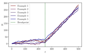
(a)

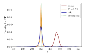
(b)

Figure 6: DGP 2: Left: Five process realisations. Right: The densities of the estimated breakpoints for each specification.

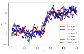
(a)

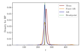
(b)

Figure 7: DGP 3: Left: Five process realisations. Right: The densities of the estimated breakpoints for each specification.

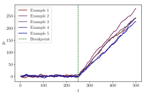
(a)

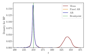
(b)

Figure 8: DGP 4: Left: Five process realisations. Right: The densities of the estimated breakpoints for each specification.

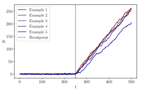
(a)

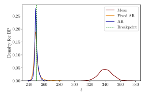
(b)

Figure 9: DGP 5: Left: Five process realisations. Right: The densities of the estimated breakpoints for each specification.

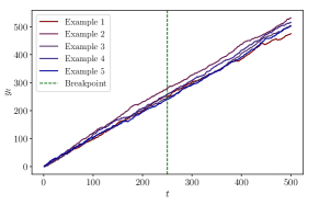
(a)

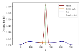
(b)

Figure 10: DGP 6: Left: Five process realisations. Right: The densities of the estimated breakpoints for each specification.

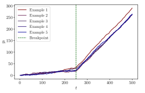
(a)

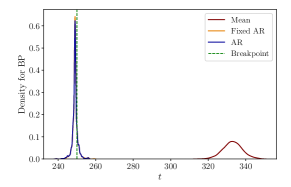
(b)

Figure 11: DGP 7: Left: Five process realisations. Right: The densities of the estimated breakpoints for each specification.

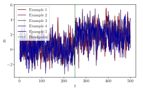
(a)

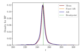
(b)

Figure 12: DGP 8: Left: Five process realisations. Right: The densities of the estimated breakpoints for each specification.

A.2 Serially correlated error term

A possible extension of the simulation study outlined in Equation (8) is allowing the error term to exhibit serial correlation. We use the same DGPs as before, but generate $\{\varepsilon_{t}\}_{t=1}^{T}$ as follows,

$$\varepsilon_{t} =\psi\varepsilon_{t-1}+\theta\eta_{t-1}+\eta_{t},\quad\eta_{t}\overset{\textit{i.i.d.}}{\sim}\mathcal{N}(0,\sigma_{\eta}^{2})\quad\forall t.$$ (9)

We conduct 1000 simulations for each, with a sample size of 500. Here, we consider DGPs 2, 3, 4, 5, 7, and 8 as outlined in Table 2 and refer to these DGPs in the serially correlated cases as models $$2_{s} 3_{s} 4_{s} 5_{s} 7_{s} 8_{s} \psi=\theta=0.5 \sigma_{\eta} \varepsilon_{t} \sigma$$, , , , , and . We set and the standard deviation , such that the standard deviation of corresponds to the in Table 2. This is accomplished as follows,

$$\operatorname{Var}\left(\varepsilon_{t}\right) =\operatorname{Var}\left(\psi\varepsilon_{t-1}+\theta\eta_{t-1}+\eta_{t}\right)$$

$$=\psi^{2}\operatorname{Var}\left(\varepsilon_{t-1}\right)+\theta^{2}\operatorname{Var}\left(\eta_{t-1}\right)+2\psi\theta\operatorname{Cov}\left(\varepsilon_{t-1},\eta_{t-1}\right)+\operatorname{Var}\left(\eta_{t}\right).$$

$$=\psi^{2}\operatorname{Var}\left(\varepsilon_{t-1}\right)+\theta^{2}\sigma_{\eta}^{2}+2\psi\theta\sigma_{\eta}^{2}+\sigma_{\eta}^{2},$$

since $$\varepsilon_{t-1} \eta_{t-1} \mathbb{E}\left[\varepsilon_{t}\eta_{t}\right]=\phi\mathbb{E}\left[\varepsilon_{t-1}\eta_{t}\right]+\theta\mathbb{E}\left[\eta_{t}\eta_{t-1}\right]+\mathbb{E}\left[\eta_{t}^{2}\right]=\sigma_{\eta}^{2} \sigma^{2}=\operatorname{Var}\left(\varepsilon_{t}\right) t$$ and have zero means and that . Given stationarity of the process, which implies for all , we derive,

$$\sigma_{\eta}^{2} =\sigma^{2}\frac{1-\psi^{2}}{1+\theta^{2}+2\psi\theta}.$$

This adjustment ensures the comparability of the results between the two error term types.

In Figures 13 through 18, we plot examples of realisations and frequency plots of the estimated breakpoints using each of the models while imposing a single breakpoint in the estimation. The results are summarised in Table 5 which provides mean of the estimated breakpoints and medians of the lower and upper boundary of the estimated confidence intervals, along with the coverage rates for each model specification and DGP. Generally speaking, the mean of the estimated breakpoints are further from the true breakpoint and the CIs become wider compared to the results from the corresponding DGPs without serial correlation. It is evident that serial correlation in the error term makes it more difficult to estimate the dating of breaks. However, we find that the Fixed AR and AR models perform well for DGPs $7_{s}$, which also has a large difference between the states and low variance. This is in line with the theoretical framework by Bai and Perron, (2003), who note that the estimated break dates are consistent even in the presence of serial correlation. Also, the Fixed AR model performs well in DGPs $2_{s}$, $4_{s}$ and $5_{s}$ with mean of the estimated breakpoints close to the true breakpoint and reasonably wide confidence intervals with acceptable coverage rates. The results of the AR model are less conclusive.

DGP	Mean				Fixed AR				AR
	BP est.	Lower	Upper	Coverage	BP est.	Lower	Upper	Coverage	BP est.	Lower	Upper	Coverage
$2_{s}$	332	-1400	335	95.9%	247	188	312	95.7%	261	190	299	79.9%
$3_{s}$	266	60	787	90.6%	285	-112	656	97.2%	276	156	421	77.1%
$4_{s}$	340	-776	339	94.9%	252	197	301	96.9%	264	195	277	84.9%
$5_{s}$	342	-329	340	96.2%	256	196	266	96.4%	259	192	250	70.8%
$7_{s}$	333	-1708	329	92.3%	249	230	270	97.6%	251	230	267	92.8%
$8_{s}$	250	122	370	98.3%	245	-5	492	99.8%	247	23	490	97.4%

Table 5: Mean of the estimated breakpoints and medians of the lower and upper boundary of the estimated confidence intervals, along with the coverage rates for each model specification and DGP.

For the Mean and Fixed AR models, the coverage rates generally are close to the desired 95% and even higher in some DGPs. However, the CIs are also extremely wide, reaching outside the sample window in many DGPs. The CIs seem reasonable in the Fixed AR model for DGPs $2_{s}$, $4_{s}$, $5_{s}$, and $7_{s}$, where the coverage rates are close to 95% and the medians of the lower and upper bounds of the CIs are not too extreme. The CIs for the AR model are generally wider than in the version without serial correlation in the error term. In the AR model, the coverage rates are lower than the desired 95%, but it seems that DGPs with large breaks have higher coverage rates. The relatively poor performance is in line with the theoretical framework by Bai and Perron, (2003). The authors note that the construction of the CIs rely on having no serial correlation in the error term if a lagged dependent variable is included as a regressor, which has coefficients that are subject to breakpoints.

DGP	Mean			Fixed AR			AR
	BIC	LWZ	KT	BIC	LWZ	KT	BIC	LWZ	KT
$2_{s}$	3.0 (0%)	3.0 (0%)	3.0 (0%)	1.9 (32%)	0.9 (70%)	2.9 (0%)	1.8 (37%)	0.7 (61%)	1.9 (33%)
$3_{s}$	3.0 (0%)	2.8 (2%)	3.0 (0%)	0.7 (33%)	0.0 (0%)	2.7 (3%)	0.3 (19%)	0.0 (0%)	0.4 (17%)
$4_{s}$	3.0 (0%)	3.0 (0%)	3.0 (0%)	1.7 (45%)	1.0 (85%)	2.8 (1%)	1.6 (51%)	0.8 (79%)	1.6 (47%)
$5_{s}$	3.0 (0%)	3.0 (0%)	3.0 (0%)	1.8 (5%)	1.1 (85%)	2.8 (0%)	1.7 (40%)	1.0 (92%)	1.6 (49%)
$7_{s}$	3.0 (0%)	3.0 (0%)	3.0 (0%)	1.9 (34%)	1.1 (89%)	3.0 (0%)	1.9 (34%)	1.0 (96%)	1.9 (32%)
$8_{s}$	2.2 (21%)	1.2 (78%)	2.2 (23%)	0.4 (35%)	0.0 (0%)	1.9 (36%)	0.0 (4%)	0.0 (0%)	0.0 (3%)

Table 6: Means of the estimated number of breakpoints for each model specification across different DGPs, rounded to one decimal. Percentages indicate the proportion of estimates equal to the true number of breakpoints.

Table 6 shows the mean number of breakpoints estimated for each DGP and method, along with the proportion of correctly estimated breakpoints. In the Mean model, all information criteria overestimate the number of breakpoints. An important exception is the eighth DGP, where the performance is better, as in the case without serial correlation. In the Fixed AR and AR model specifications, the LWZ criterion generally performs well, while both the BIC and the KT criteria generally overestimate the number of breakpoints. However, the LWZ criterion leads to underestimating the number of breakpoints in DGPs $3_{s}$ and $8_{s}$. These two DGPs are characterised by fixed AR-coefficients which are lower than one. This implies that these two processes do not exhibit an autoregressive unit root. Hence, it seems that the LWZ criterion performs well in cases of state-wise unit roots or switching between stationary and non-stationary states.

Compared to the findings in the DGPs without serial correlation, it is clear that the proportion of correct estimates are lower for most DGPs and model specifications. Overall, the best performing criterion seems to be the LWZ criterion in the Fixed AR and AR models, while the Mean model typically leads to overestimating the number of breakpoints.

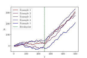
(a)

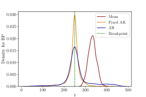
(b)

Figure 13: DGP $2_{s}$: Left: Five process realisations. Right: The densities of the estimated breakpoints for each specification.

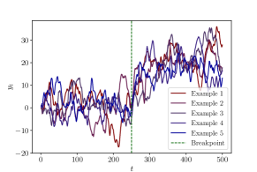
(a)

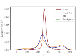
(b)

Figure 14: DGP $3_{s}$: Left: Five process realisations. Right: The densities of the estimated breakpoints for each specification.

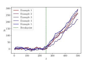
(a)

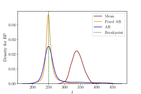
(b)

Figure 15: DGP $4_{s}$: Left: Five process realisations. Right: The densities of the estimated breakpoints for each specification.

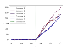
(a)

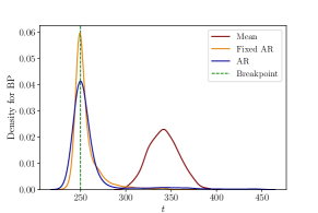
(b)

Figure 16: DGP $5_{s}$: Left: Five process realisations. Right: The densities of the estimated breakpoints for each specification.

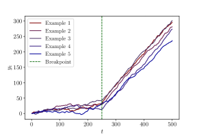
(a)

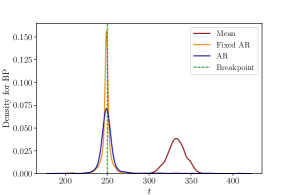
(b)

Figure 17: DGP $7_{s}$: Left: Five process realisations. Right: The densities of the estimated breakpoints for each specification.

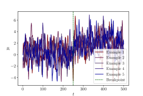
(a)

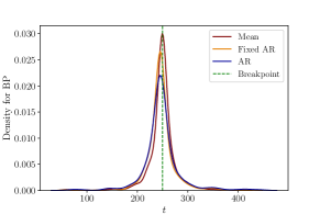
(b)

Figure 18: DGP $8_{s}$: Left: Five process realisations. Right: The densities of the estimated breakpoints for each specification.

Appendix B Graphs

B.1 1 to 15 breakpoints

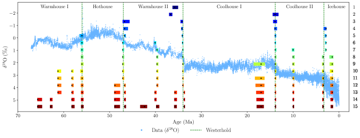
Figure 19: A comparison of estimated breakpoints using the Fixed AR model for 1 to 15 breakpoints on 25 kyr binned data. This is estimated using a minimum state length of 1 Myr. The black dots represent estimated breakpoints, while coloured shaded rectangles indicate 95% confidence intervals. The results overlay the $\delta^{18}$O data from Westerhold et al., (2020) and their climate states.

B.2 Reversed time

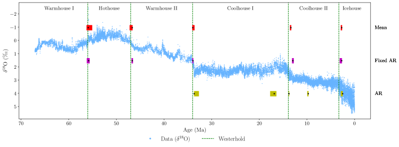
Figure 20: A comparison of estimated breakpoints using the Mean, Fixed AR, and AR model specifications for 5 breakpoints on 25 kyr binned data where the time frame is reversed. The black dots represent estimated breakpoints, while coloured shaded rectangles indicate 95% confidence intervals. The results overlay the $\delta^{18}$O data from Westerhold et al., (2020) and their climate states.

B.3 Comparing the frequency: 3 breakpoints

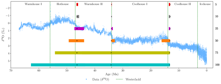
(a) Mean model

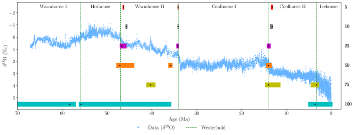
(b) Fixed AR model

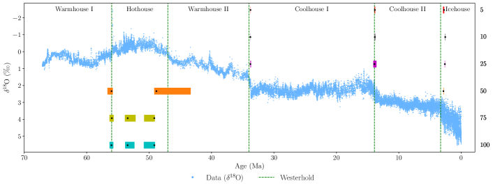
(c) AR model

Figure 21: A comparison of estimated breakpoints using binned data with frequencies of 5, 10, 25, 50, 75, and 100 kyr from top to bottom, fixing the number of breakpoints to 3 for each model specification. The black dots represent estimated breakpoints, while coloured shaded rectangles indicate 95% confidence intervals. The results overlay the $\delta^{18}$O data from Westerhold et al., (2020) and their climate states.

B.4 Comparing the frequency: 7 breakpoints

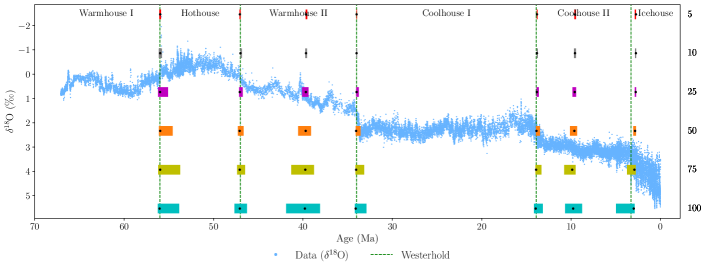
(a) Mean model

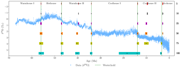
(b) Fixed AR model

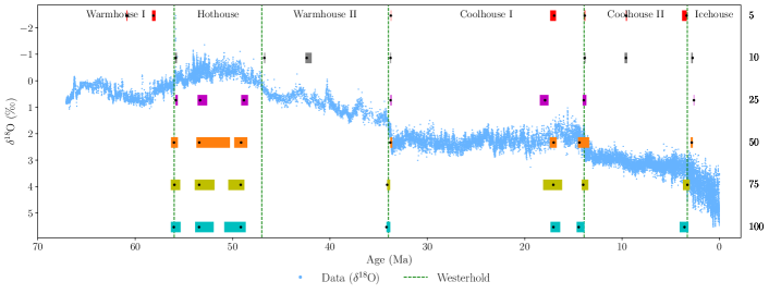
(c) AR model

Figure 22: A comparison of estimated breakpoints using binned data with frequencies of 5, 10, 25, 50, 75, and 100 kyr from top to bottom, fixing the number of breakpoints to 7 for each model specification. The black dots represent estimated breakpoints, while coloured shaded rectangles indicate 95% confidence intervals. The results overlay the $\delta^{18}$O data from Westerhold et al., (2020) and their climate states.

Appendix C Tables

C.1 Summary statistics: State-wise and full sample

Bin size	State	Mean	Sd.	Max.	Min.	Data points
5	Icehouse	4.037	0.463	5.405	3.05	660
5	Coolhouse II	3.072	0.237	4.172	1.885	2120
5	Coolhouse I	2.239	0.233	2.991	1.266	4020
5	Warmhouse II	0.897	0.366	1.894	-0.254	2600
5	Hothouse	-0.269	0.261	0.391	-2.014	1800
5	Warmhouse I	0.417	0.249	1.07	-0.215	2221
5	Full sample period	1.561	1.277	5.405	-2.014	13421
10	Icehouse	4.034	0.447	5.33	3.181	330
10	Coolhouse II	3.072	0.228	4.122	1.975	1060
10	Coolhouse I	2.239	0.221	2.877	1.324	2010
10	Warmhouse II	0.897	0.366	1.777	-0.254	1300
10	Hothouse	-0.269	0.256	0.308	-2.014	900
10	Warmhouse I	0.417	0.245	0.977	-0.12	1111
10	Full sample period	1.561	1.276	5.33	-2.014	6711
25	Icehouse	4.033	0.401	5.158	3.258	132
25	Coolhouse II	3.073	0.213	3.793	2.087	424
25	Coolhouse I	2.239	0.202	2.749	1.391	804
25	Warmhouse II	0.898	0.358	1.688	0.01	520
25	Hothouse	-0.269	0.245	0.218	-1.871	360
25	Warmhouse I	0.418	0.237	0.912	-0.065	445
25	Full sample period	1.561	1.273	5.158	-1.871	2685
50	Icehouse	4.042	0.359	4.757	3.264	66
50	Coolhouse II	3.072	0.206	3.72	2.156	212
50	Coolhouse I	2.24	0.188	2.713	1.567	402
50	Warmhouse II	0.898	0.354	1.656	0.182	260
50	Hothouse	-0.268	0.233	0.197	-1.871	180
50	Warmhouse I	0.419	0.233	0.867	-0.042	223
50	Full sample period	1.562	1.271	4.757	-1.871	1343
75	Icehouse	4.041	0.351	4.753	3.283	44
75	Coolhouse II	3.068	0.214	3.652	2.072	142
75	Coolhouse I	2.239	0.181	2.717	1.691	268
75	Warmhouse II	0.894	0.351	1.553	0.156	173
75	Hothouse	-0.26	0.203	0.167	-0.985	120
75	Warmhouse I	0.42	0.229	0.837	0.006	148
75	Full sample period	1.563	1.268	4.753	-0.985	895
100	Icehouse	4.047	0.344	4.673	3.4	33
100	Coolhouse II	3.073	0.201	3.625	2.353	106
100	Coolhouse I	2.241	0.175	2.685	1.739	201
100	Warmhouse II	0.898	0.349	1.601	0.228	130
100	Hothouse	-0.263	0.203	0.155	-0.985	90
100	Warmhouse I	0.42	0.229	0.832	0.007	112
100	Full sample period	1.562	1.269	4.673	-0.985	672
Without binning	Icehouse	4.064	0.533	5.53	2.66	3731
Without binning	Coolhouse II	3.102	0.254	4.49	1.84	6282
Without binning	Coolhouse I	2.251	0.242	3.263	1.026	6669
Without binning	Warmhouse II	0.916	0.357	1.894	-0.254	1786
Without binning	Hothouse	-0.279	0.255	0.391	-2.46	3030
Without binning	Warmhouse I	0.428	0.25	1.07	-0.215	2761
Without binning	Full sample period	2.128	1.445	5.53	-2.46	24259

Table 7: Summary statistics of the binned data with bin sizes (5, 10, 25, 50, 75, and 100 kyr) and the $\delta^{18}$O data without binning for each of the states identified by Westerhold et al., (2020) and the full sample period.

C.2 Double maximum test

Model	UDMax	10% CV	5% CV	2.5% CV	1% CV
Mean	1522.778	8.78	10.17	11.52	13.74
Fixed AR	34.208	8.78	10.17	11.52	13.74
AR	75.619	11.69	13.27	14.69	16.79

Table 8: Test statistics from the double maximum test for each model specification, alongside the critical values. They are estimated on the 25 kyr binned data, $\varepsilon$ is set to 5%, and the maximum number of breakpoints is 8.

C.3 Estimated breakpoints: 3 breakpoints

Bin size	BP index	Mean		Fixed AR		AR
		Estimate	95% CI	Estimate	95% CI	Estimate	95% CI
5	1	46.34	(46.55, 46.0)	46.38	(46.52, 46.2)	33.76	(33.76, 33.74)
5	2	34.02	(34.03, 33.93)	34.16	(34.24, 34.1)	13.83	(13.88, 13.78)
5	3	13.1	(13.53, 13.09)	13.15	(13.45, 13.05)	2.75	(2.91, 2.73)
10	1	46.35	(46.51, 45.63)	45.73	(45.89, 45.45)	33.78	(33.78, 33.75)
10	2	34.03	(34.04, 33.93)	34.16	(34.27, 34.08)	13.84	(13.94, 13.74)
10	3	13.1	(13.54, 13.08)	13.16	(13.62, 13.02)	2.56	(2.62, 2.54)
25	1	46.37	(47.29, 43.84)	46.74	(47.16, 45.64)	33.77	(33.77, 33.67)
25	2	34.05	(34.07, 33.57)	34.25	(34.55, 34.02)	13.91	(14.09, 13.59)
25	3	13.12	(13.54, 13.07)	13.94	(14.36, 13.51)	2.62	(2.65, 2.6)
50	1	46.38	(49.33, 43.83)	47.13	(47.93, 43.93)	56.02	(56.67, 55.82)
50	2	34.1	(34.1, 32.85)	35.8	(36.35, 35.4)	48.83	(49.18, 43.34)
50	3	13.18	(16.13, 13.13)	13.98	(14.53, 13.28)	2.85	(2.85, 2.8)
75	1	46.4	(54.25, 41.76)	40.33	(41.23, 39.21)	55.97	(56.35, 55.68)
75	2	34.12	(34.12, 30.98)	13.99	(14.74, 11.3)	53.43	(53.88, 52.16)
75	3	13.25	(44.53, 13.17)	3.29	(4.56, 2.69)	49.17	(50.81, 49.09)
100	1	46.36	(62.81, 43.47)	58.33	(90.73, 56.93)	56.03	(56.33, 55.73)
100	2	34.2	(34.2, 27.92)	55.83	(56.33, 35.69)	53.44	(53.84, 52.34)
100	3	13.26	(54.24, 13.16)	3.59	(5.08, -0.3)	49.15	(50.85, 49.05)

Table 9: Estimated breakpoints and their 95% confidence intervals (in Ma) where the number of breakpoints is fixed to 3, and all values are rounded to two decimals. Estimates for each method across bin sizes 5, 10, 25, 50, 75, and 100 kyr.

C.4 Estimated breakpoints: 5 breakpoints

Bin size	BP index	Mean		Fixed AR		AR
		Estimate	95% CI	Estimate	95% CI	Estimate	95% CI
5	1	55.97	(56.09, 55.89)	56	(56.09, 55.92)	33.75	(33.75, 33.72)
5	2	46.73	(46.85, 46.68)	46.73	(46.76, 46.68)	16.97	(17.37, 16.79)
5	3	34.02	(34.03, 33.92)	34.05	(34.08, 34.02)	13.83	(13.85, 13.78)
5	4	13.37	(13.4, 13.33)	13.42	(13.47, 13.35)	9.56	(9.59, 9.51)
5	5	2.74	(2.85, 2.72)	2.75	(3.11, 2.72)	3.37	(3.82, 3.36)
10	1	55.97	(56.15, 55.79)	55.99	(56.15, 55.88)	33.78	(33.78, 33.73)
10	2	46.74	(46.85, 46.65)	46.74	(46.78, 46.65)	17.89	(18.33, 17.65)
10	3	34.03	(34.04, 33.91)	34.16	(34.19, 34.1)	13.84	(13.86, 13.77)
10	4	13.38	(13.42, 13.32)	13.84	(13.91, 13.74)	9.61	(9.74, 9.47)
10	5	2.75	(2.83, 2.72)	2.76	(3.2, 2.73)	2.76	(2.9, 2.74)
25	1	55.98	(56.31, 55.11)	56.03	(56.58, 55.71)	55.83	(55.86, 55.68)
25	2	46.74	(47.31, 46.57)	46.74	(46.84, 46.47)	48.36	(48.64, 47.86)
25	3	34.05	(34.07, 33.53)	34.17	(34.25, 34.02)	33.77	(33.77, 33.7)
25	4	13.44	(13.56, 13.32)	13.91	(14.01, 13.69)	13.91	(14.09, 13.59)
25	5	2.77	(2.85, 2.67)	2.82	(3.12, 2.75)	2.62	(2.65, 2.6)
50	1	55.97	(56.22, 54.62)	56.02	(57.11, 55.37)	56.02	(56.67, 55.72)
50	2	46.73	(48.18, 46.48)	47.13	(47.28, 46.58)	48.83	(49.13, 40.49)
50	3	34.1	(34.1, 32.85)	34.25	(34.35, 33.95)	33.8	(33.8, 33.65)
50	4	13.88	(14.23, 13.68)	13.93	(14.08, 13.53)	17.02	(17.42, 16.77)
50	5	2.85	(3.0, 2.6)	3.25	(3.49, 3.1)	14.38	(14.63, 12.88)
75	1	55.97	(56.35, 53.8)	56.27	(57.47, 54.78)	55.97	(56.35, 55.53)
75	2	46.77	(50.66, 46.47)	47.14	(47.52, 46.47)	53.36	(53.65, 50.14)
75	3	34.12	(34.12, 30.98)	34.27	(34.5, 33.75)	34.12	(34.12, 33.9)
75	4	13.47	(13.92, 13.1)	13.99	(14.22, 13.25)	17.06	(17.44, 16.61)
75	5	2.92	(3.52, 2.54)	3.29	(3.67, 3.07)	14.59	(15.19, 14.37)
100	1	56.03	(56.43, 54.04)	56.23	(57.73, 54.54)	56.03	(56.33, 55.53)
100	2	46.76	(52.54, 46.36)	47.16	(47.76, 46.36)	53.44	(53.84, 52.14)
100	3	34.2	(34.2, 29.51)	34.3	(34.6, 33.5)	49.15	(50.85, 48.85)
100	4	13.96	(14.86, 13.56)	14.06	(14.26, 13.06)	34.2	(34.2, 33.9)
100	5	3.09	(4.39, 2.49)	3.59	(3.99, 3.39)	13.96	(15.85, 13.06)

Table 10: Estimated breakpoints and their 95% confidence intervals (in Ma) where the number of breakpoints is fixed to 5, and all values are rounded to two decimals. The table shows estimates for each method across bin sizes 5, 10, 25, 50, 75, and 100 kyr.

C.5 Estimated breakpoints: 7 breakpoints

Bin size	BP index	Mean		Fixed AR		AR
		Estimate	95% CI	Estimate	95% CI	Estimate	95% CI
5	1	55.97	(56.06, 55.88)	56	(56.05, 55.93)	60.84	(60.87, 60.8)
5	2	47.05	(47.1, 46.97)	47.12	(47.14, 47.06)	58.14	(58.27, 57.91)
5	3	39.65	(39.7, 39.51)	39.65	(39.69, 39.58)	33.75	(33.75, 33.72)
5	4	33.99	(34.01, 33.95)	34.02	(34.05, 33.99)	16.97	(17.37, 16.79)
5	5	13.82	(13.84, 13.76)	13.83	(13.88, 13.75)	13.83	(13.85, 13.78)
5	6	9.56	(9.63, 9.46)	9.6	(9.77, 9.41)	9.56	(9.59, 9.51)
5	7	2.74	(2.88, 2.73)	2.75	(3.0, 2.73)	3.37	(3.82, 3.36)
10	1	55.97	(56.12, 55.77)	55.99	(56.08, 55.88)	55.83	(55.9, 55.72)
10	2	46.99	(47.01, 46.84)	47.13	(47.16, 47.02)	46.74	(46.75, 46.67)
10	3	39.66	(39.74, 39.55)	39.66	(39.71, 39.55)	42.39	(42.52, 41.88)
10	4	34	(34.03, 33.93)	34.03	(34.07, 33.97)	33.78	(33.8, 33.73)
10	5	13.83	(13.85, 13.73)	13.84	(13.9, 13.73)	13.84	(13.87, 13.77)
10	6	9.57	(9.68, 9.46)	9.61	(9.79, 9.37)	9.61	(9.74, 9.47)
10	7	2.75	(2.85, 2.73)	2.76	(3.06, 2.74)	2.76	(2.9, 2.74)
25	1	55.98	(56.21, 55.08)	56.03	(56.31, 55.71)	55.83	(55.86, 55.63)
25	2	47.06	(47.14, 46.74)	47.14	(47.19, 46.84)	53.34	(53.59, 52.61)
25	3	39.67	(40.1, 39.37)	39.67	(39.8, 39.42)	48.84	(49.11, 48.41)
25	4	34	(34.05, 33.75)	34.05	(34.12, 33.9)	33.77	(33.77, 33.67)
25	5	13.84	(13.86, 13.61)	13.91	(13.96, 13.64)	17.91	(18.44, 17.56)
25	6	9.59	(9.84, 9.44)	10.02	(10.29, 9.74)	13.94	(14.04, 13.66)
25	7	2.77	(2.87, 2.72)	2.82	(3.05, 2.77)	2.62	(2.65, 2.6)
50	1	55.97	(56.12, 54.57)	56.02	(56.52, 55.42)	56.02	(56.32, 55.62)
50	2	47.08	(47.28, 46.63)	47.13	(47.18, 46.53)	53.42	(53.72, 50.28)
50	3	39.69	(40.54, 39.09)	40.29	(40.59, 39.89)	49.13	(49.83, 48.48)
50	4	34.05	(34.1, 33.55)	34.1	(34.2, 33.8)	33.8	(33.8, 33.6)
50	5	13.88	(13.93, 13.48)	13.93	(14.03, 13.53)	17.02	(17.42, 16.73)
50	6	9.64	(10.13, 9.34)	10.04	(10.53, 9.64)	14.38	(14.53, 13.38)
50	7	2.85	(3.05, 2.75)	2.85	(3.0, 2.75)	2.85	(2.95, 2.75)
75	1	55.97	(56.2, 53.73)	56.2	(56.8, 55.08)	55.97	(56.35, 55.38)
75	2	47.07	(47.37, 46.47)	47.14	(47.37, 46.32)	53.43	(53.88, 51.86)
75	3	39.74	(41.31, 38.76)	40.33	(40.78, 39.51)	49.17	(50.44, 48.79)
75	4	34.05	(34.12, 33.15)	34.12	(34.35, 33.67)	34.12	(34.12, 33.82)
75	5	13.92	(13.99, 13.32)	13.99	(14.14, 13.25)	17.06	(18.11, 16.16)
75	6	9.88	(10.78, 9.5)	10.1	(11.0, 9.05)	13.99	(14.14, 13.47)
75	7	2.92	(3.74, 2.77)	3.29	(3.67, 3.14)	3.29	(3.74, 3.07)
100	1	56.03	(56.23, 53.84)	56.23	(57.03, 54.74)	56.03	(56.33, 55.34)
100	2	47.06	(47.66, 46.26)	47.16	(47.36, 46.16)	53.44	(53.84, 51.95)
100	3	39.78	(41.88, 38.09)	40.28	(41.08, 39.18)	49.15	(50.85, 48.65)
100	4	34.1	(34.2, 32.9)	34.3	(34.6, 33.6)	34.2	(34.2, 33.8)
100	5	13.96	(14.16, 13.16)	18.45	(22.03, 12.76)	17.05	(17.35, 16.35)
100	6	9.77	(10.67, 8.77)	14.06	(14.16, 13.66)	14.46	(14.66, 13.86)
100	7	2.99	(4.99, 2.89)	3.59	(3.99, 3.39)	3.59	(4.09, 3.19)

Table 11: Estimated breakpoints and their 95% confidence intervals (in Ma) where the number of breakpoints is fixed to 7, and all values are rounded to two decimals. The table shows estimates for each model across bin sizes 5, 10, 25, 50, 75, and 100 kyr.

References

- Andrews, (1991) Andrews, D. W. K. (1991). Heteroskedasticity and Autocorrelation Consistent Covariance Matrix Estimation. Econometrica, 59(3):817–858.
- Andrews and Monahan, (1992) Andrews, D. W. K. and Monahan, J. C. (1992). An Improved Heteroskedasticity and Autocorrelation Consistent Covariance Matrix Estimator. Econometrica, 60(4):953–966.
- Bai and Perron, (1998) Bai, J. and Perron, P. (1998). Estimating and Testing Linear Models with Multiple Structural Changes. Econometrica, 66(1):47–78.
- Bai and Perron, (2003) Bai, J. and Perron, P. (2003). Computation and analysis of multiple structural change models. Journal of Applied Econometrics, 18(1):1–22.
- Bai and Perron, (2006) Bai, J. and Perron, P. (2006). Multiple Structural Change Models: A Simulation Analysis, page 212–238. Cambridge University Press.
- Bennedsen et al., (2024) Bennedsen, M., Hillebrand, E., Larsen, K., and Koopman, S. J. (2024). Continuous-time state-space time series models for O and C. Abstract submitted to EGU General Assembly Session NP3.3. European Geosciences Union General Assembly 2024.
- Boettner et al., (2021) Boettner, C., Klinghammer, G., Boers, N., Westerhold, T., and Marwan, N. (2021). Early-warning signals for Cenozoic climate transitions. Quaternary Science Reviews, 270:107177.
- CenCO2PIP Consortium, (2023) CenCO2PIP Consortium (2023). The Cenozoic CO2 Proxy Integration Project (CenCO2PIP) Consortium: Hönisch, B., Royer, D. L., Breecker, D. O., Polissar, P. J., Bowen, G. J., Henehan, M. J., Cui, Y., Steinthorsdottir, M., McElwain, J. C., Kohn, M. J., Pearson, A., Phelps, S. R., Uno, K. T., Ridgwell, A., Anagnostou, E., Austermann, J., Badger, M. P. S., Barclay, R. S., Bijl, P. K., Chalk, T. B., Scotese, C. R., de la Vega, E., DeConto,c R. M., Dyez, K. A., Ferrini, V., Franks, P. J., Giulivi, C. F., Gutjahr, M., Harper, D. T., Haynes, L. L., Huber, M., Snell, K. E., Keisling, B. A., Konrad, W., Lowenstein, T. K., Malinverno, A., Guillermic, M., Mejía, L. M., Milligan, J. N., Morton, J. J., Nordt, L., Whiteford, R., Roth-Nebelsick, A., Rugenstein, J. K. C., Schaller, M. F., Sheldon, N. D., Sosdian, S., Wilkes, E. B., Witkowski, C. R., Zhang, Y. G., Anderson, L., Beerling, D. J., Bolton, C., Cerling, T. E., Cotton, J. M., Da, J., Ekart, D. D., Foster, G. L., Greenwood, D. R., Hyland, E. G., Jagniecki, E. A., Jasper, J. P., Kowalczyk, J. B., Kunzmann, L., Kürschner, and W. M., Lawrence, C. E., Lear, C. H., Martínez-Botí, M. A., Maxbauer, D. P., Montagna, P., Naafs, B. D. A., Rae, J. W. B., Raitzsch, M., Retallack, G. J., Ring, S. J., Seki, O., Sepúlveda, J., Sinha, A., Tesfamichael, T. F., Tripati, A., van der Burgh, J., Yu, J., Zachos, J. C. and Zhang, L. Toward a Cenozoic history of atmospheric CO2. Science, 382(6675):eadi5177.
- Dickey and Fuller, (1979) Dickey, D. and Fuller, W. (1979). Distribution of the Estimators for Autoregressive Time Series With a Unit Root. Journal of the American Statistical Association, 74.
- Epstein et al., (1951) Epstein, S., Buchsbaum, R., Lowenstam, H., and Urey, H. C. (1951). Carbonate-Water Isotopic Temperature Scale. GSA Bulletin, 62(4):417–426.
- Goswami et al., (2018) Goswami, B., Boers, N., Rheinwalt, A., Marwan, N., Heitzig, J., Breitenbach, S., and Kurths, J. (2018). Abrupt transitions in time series with uncertainties. Nature Communications, 9(48).
- Kejriwal et al., (2013) Kejriwal, M., Perron, P., and Zhou, J. (2013). Wald tests for detecting multiple structural changes in persistence. Econometric Theory, 29(2):289–323.
- Kurozumi and Tuvaandorj, (2011) Kurozumi, E. and Tuvaandorj, P. (2011). Model selection criteria in multivariate models with multiple structural changes. Journal of Econometrics, 164(2):218–238.
- Kwiatkowski et al., (1992) Kwiatkowski, D., Phillips, P. C., Schmidt, P., and Shin, Y. (1992). Testing the null hypothesis of stationarity against the alternative of a unit root: How sure are we that economic time series have a unit root? Journal of Econometrics, 54(1):159–178.
- Liu et al., (1997) Liu, J., Wu, S., and Zidek, J. V. (1997). On Segmented Multivariate Regressions. Statistica Sinica, 7:497–525.
- Livina et al., (2010) Livina, V. N., Kwasniok, F., and Lenton, T. M. (2010). Potential analysis reveals changing number of climate states during the last 60 kyr. Climate of the Past, 6(1):77–82.
- Marwan, (2023) Marwan, N. (2023). Challenges and perspectives in recurrence analyses of event time series. Frontiers in Applied Mathematics and Statistics, 9.
- Marwan et al., (2007) Marwan, N., Carmen Romano, M., Thiel, M., and Kurths, J. (2007). Recurrence plots for the analysis of complex systems. Physics Reports, 438(5):237–329.
- Marwan et al., (2021) Marwan, N., Donges, J. F., Donner, R. V., and Eroglu, D. (2021). Nonlinear time series analysis of palaeoclimate proxy records. Quaternary Science Reviews, 274:107245.
- Nguyen et al., (2023) Nguyen, L., Yamamoto, Y., and Perron, P. (2023). mbreaks: Estimation and Inference for Structural Breaks in Linear Regression Models. R package version 1.0.0.
- Reikard, (2021) Reikard, G. (2021). Forecasting paleoclimatic data with time series models. Results in Geophysical Sciences, 6:100015.
- Rousseau et al., (2023) Rousseau, D.-D., Bagniewski, W., and Lucarini, V. (2023). A Punctuated Equilibrium Analysis of the Climate Evolution of Cenozoic Exhibits a Hierarchy of Abrupt Transitions. Scientific Reports, 13:11290.
- Ruggieri, (2013) Ruggieri, E. (2013). A Bayesian approach to detecting change points in climatic records. International Journal of Climatology, 33(2):520–528.
- Shackleton, (1967) Shackleton, N. (1967). Oxygen Isotope Analyses and Pleistocene Temperatures Re-assessed. Nature, 215:15–17.
- Tierney et al., (2020) Tierney, J. E., Poulsen, C. J., Montañez, I. P., Bhattacharya, T., Feng, R., Ford, H. L., Hönisch, B., Inglis, G. N., Petersen, S. V., Sagoo, N., Tabor, C. R., Thirumalai, K., Zhu, J., Burls, N. J., Foster, G. L., Goddéris, Y., Huber, B. T., Ivany, L. C., Turner, S. K., Lunt, D. J., McElwain, J. C., Mills, B. J. W., Otto-Bliesner, B. L., Ridgwell, A., and Zhang, Y. G. (2020). Past climates inform our future. Science, 370(6517):eaay3701.
- Westerhold et al., (2020) Westerhold, T., Marwan, N., Drury, A. J., Liebrand, D., Agnini, C., Anagnostou, E., Barnet, J. S. K., Bohaty, S. M., Vleeschouwer, D. D., Florindo, F., Frederichs, T., Hodell, D. A., Holbourn, A. E., Kroon, D., Lauretano, V., Littler, K., Lourens, L. J., Lyle, M., Pälike, H., Röhl, U., Tian, J., Wilkens, R. H., Wilson, P. A., and Zachos, J. C. (2020). An astronomically dated record of Earth’s climate and its predictability over the last 66 million years. Science, 369(6509):1383–1387.
- Yao, (1988) Yao, Y.-C. (1988). Estimating the number of change-points via Schwarz’ criterion. Statistics & Probability Letters, 6(3):181–189.
- Zachos et al., (2001) Zachos, J., MO, P., Sloan, L., Thomas, E., and Billups, K. (2001). Trends, Rhythms, and Aberrations in Global Climate 65 Ma to Present. Science (New York, N.Y.), 292:686–93.