Wigner kernel and Gabor matrix of operators

Abstract.

We exhibit the connection between the Wigner kernel and the Gabor matrix of a linear bounded operator $T:\mathcal{S}(\mathbb{R}^{d})\to\mathcal{S}^{\prime}(\mathbb{R}^{d})$. The smoothing effect of the Gabor matrix is highlighted by basic examples. This connection allows a comparison between the classes of Fourier integral operators defined by means of the Gabor matrix in [8] and the Wigner kernel in [6], showing the nice off-diagonal decay of the Gabor class with respect to the Wigner kernel one and suggesting further investigations. Modulation spaces containing the Sjöstrand class are the symbol classes of this study.

1. Introduction

The Gabor matrix of an operator was introduced by Gröchenig in the pioneering work [15] for the study of pseudodifferential operators and later extended to Fourier integral operators in [9]. These two papers paved the way to many subsequent articles with applications to PDE’s and Quantum Mechanics. The contributions are so many that it is impossible to cite them all (cf. the textbook [10] for a partial list). Recently, evolution equations and dynamical version of Hardy uncertainty principles [18] have suggested to look at the Wigner kernel of an operator, introduced and studied in [5, 6]. We want here to establish a connection between it and the Gabor matrix.

To introduce these features properly, we need to present first some basic elements of time-frequency  analysis.

Given $z=(x,\xi)\in{\mathbb{R}^{2d}}$, we define the related time-frequency shift  acting on a function or distribution $f$ on $\mathbb{R}^{d}$ as

(1) $$\pi(z)f(t)=M_{\xi}T_{x}f(t)=e^{2\pi i\xi t}f(t-x),\,\quad t\in\mathbb{R}^{d}.$$

The short-time Fourier transform (STFT) $V_{g}f$ of a function/tempered distribution $f$ in $\mathcal{S}^{\prime}(\mathbb{R}^{d})$ with respect to the the window $g\in\mathcal{S}(\mathbb{R}^{d})\setminus\{0\}$ is defined by

$$V_{g}f(x,\xi)=\langle f,M_{\xi}T_{x}g\rangle=\int e^{-2\pi i\xi y}f(y)\overline{g(y-x)}\,dy,$$

(i.e., the Fourier transform $\mathcal{F}$ applied to $f\overline{T_{x}g}$).

The STFT enjoys the following inversion formula [10, Thrm. 1.2.16]: assume $g,\gamma\in L^{2}(\mathbb{R}^{d})$, with $\langle g,\gamma\rangle\not=0$. Then, for all $f\in L^{2}(\mathbb{R}^{d})$, in terms of vector-valued integrals,

(2) $$f=\frac{1}{\langle\gamma,g\rangle}\int_{\mathbb{R}^{2d}}V_{g}f(z)\pi(z)\gamma\,dz\,.$$

The adjoint operator of $V_{\gamma}$, defined by

$$V_{\gamma}^{\ast}F(t)=\int_{{\mathbb{R}^{2d}}}F(z)\pi(z)\gamma dz\,,\quad F\in L^{2}({\mathbb{R}^{2d}}),$$

maps $L^{2}({\mathbb{R}^{2d}})$ into $L^{2}(\mathbb{R}^{d})$. In particular, if $F=V_{g}f$ the inversion formula (2) can be rephrased as

(3) $${\rm Id}_{L^{2}}=\frac{1}{\langle\gamma,g\rangle}V_{\gamma}^{\ast}V_{g}.$$

Definition 1.1.

Fix $g,\gamma\in\mathcal{S}(\mathbb{R}^{d})\setminus\{0\}$. The Gabor matrix of a linear continuous operator $T$ from $\mathcal{S}(\mathbb{R}^{d})$ to $\mathcal{S}^{\prime}(\mathbb{R}^{d})$ is defined to be

(4) $$\langle T\pi(z)g,\pi(w)\gamma\rangle,\quad z,w\in{\mathbb{R}^{2d}}.$$

The Gabor matrix can be viewed as a kernel of an integral operator. For simplicity, choose $g,\gamma\in\mathcal{S}(\mathbb{R}^{d})$ such that $\langle\gamma,g\rangle=1$ and the inversion formula (3) becomes $V_{\gamma}^{\ast}V_{g}={\rm Id}$ (or, switching $g$ and $\gamma$, $V_{g}^{\ast}V_{\gamma}={\rm Id}$). A linear and bounded operator $T:\mathcal{S}(\mathbb{R}^{d})\to\mathcal{S}^{\prime}(\mathbb{R}^{d})$ can be written as

(5) $$T=V_{\gamma}^{\ast}V_{g}TV_{\gamma}^{\ast}V_{g}\,.$$

The linear transformation $V_{g}TV_{\gamma}^{\ast}$ is an integral operator whose kernel coincides with the Gabor matrix of $T$:

$$K_{T,g,\gamma}(w,z)=\langle T\pi(z)g,\pi(w)\gamma\rangle,\quad\,\,w,z\in{\mathbb{R}^{2d}}.$$

Estimates in the sequel will not depend on the choice of $g,\gamma$, and one can limit attention to the case $g=\gamma$, cf. [10]. For sake of generality, we shall work with the former case, viewing the latter as special case when $\gamma=g$.

The Gabor matrix approach was successfully used to characterize algebras of pseudodifferential operators by Gröchenig in [15] and later with Rzeszotnik in [16]:

(6) $$\sigma^{w}f(x)=\int_{{\mathbb{R}^{2d}}}e^{2\pi ix\xi}\sigma\left(\frac{x+y}{2},\xi\right)dyd\xi.$$

The symbol class object of their investigation is the so-called Sjöstrand class or modulation space

(7) $$S_{w}=M^{\infty,1}({\mathbb{R}^{2d}}),$$

of symbols $\sigma$ such that, for a fixed window $G\in\mathcal{S}({\mathbb{R}^{2d}})\setminus\{0\}$,

$$\int_{\mathbb{R}^{d}}\sup_{z\in\mathbb{R}^{d}}|\langle\sigma,\pi(z,\zeta)G\rangle|\,d\zeta<\infty.$$

The following related scale of spaces were considered, too:

(8) $$S^{s}_{w}=M^{\infty,\infty}_{1\otimes v_{s}}({\mathbb{R}^{2d}}),\quad v_{s}(z)=(1+|z|^{2})^{s/2},\,\,z\in{\mathbb{R}^{2d}},$$

of symbols $\sigma$ satisfying

$$\sup_{z,\zeta\in\mathbb{R}^{d}}|\langle\sigma,\pi(z,\zeta)G\rangle|v_{s}(\zeta)\,<\infty,$$

with the parameter $s\in[0,\infty)$, see details in the next Section $2.1$.

Notice that the regularity of the spaces $S^{s}_{w}$ increases with $s$ whereas in the maximal space $S_{w}$ even differentiability is lost [2, 10, 14]. Our attention in the sequel will be focused on the scale (7).

The characterization of pseudodifferential operators was further extended to Fourier integral operators (FIOs) of Schrödinger type in [8], constructing Wiener subalgebras of FIOs with symbols in $S^{s}_{w}$. This paper paved the way to many other contributions in this framework, addressing regularity properties of FIOs by means of the off-diagonal decay of their Gabor matrix, cf. [10, Chapter 5] for a partial list of references.

Precisely, a class of FIOs associated to a canonical transformation $\chi$ (cf. Definition 2.1 below) was constructed as follows (we refer to Section $2$ for the properties of $\chi$).

Definition 1.2.

Let $\chi$ be a canonical transformation satisfying B1 and B2 in Definition 2.1, and $s\geq 0$. Fix $g\in\mathcal{S}(\mathbb{R}^{d})\setminus\{0\}$. We say that a continuous linear operator $T:\mathcal{S}(\mathbb{R}^{d})\to\mathcal{S}^{\prime}(\mathbb{R}^{d})$ is in the class $FIO_{\mathcal{G}}(\chi,s)$, if its Gabor matrix satisfies the decay condition

(9) $$|\langle T\pi(z)g,\pi(w)g\rangle|\leq{C}\langle w-\chi(z)\rangle^{-s},\qquad\forall\,w,z\in{\mathbb{R}^{2d}}.$$

If the study is limited to FIOs of type I with symbol $\sigma\in\mathcal{S}^{\prime}({\mathbb{R}^{2d}})$ and tame phase $\Phi$ (Definition 2.1), namely to operators formally written as

(10) $$Tf(x)=T_{I,\Phi,\sigma}f(x)=\int_{\mathbb{R}^{d}}e^{2\pi i\Phi(x,\xi)}\sigma(x,\xi)\widehat{f}(\xi)\,d\xi\,,\quad f\in\mathcal{S}(\mathbb{R}^{d}),$$

then the characterization involves the symbol classes $S^{s}_{w}$ as follows:

Theorem 1.3 ([9, 10]).

Fix $g\in\mathcal{S}(\mathbb{R}^{d})\setminus\{0\}$ and $s\geq 0$. Let $T$ be a continuous linear operator $\mathcal{S}(\mathbb{R}^{d})\to\mathcal{S}^{\prime}(\mathbb{R}^{d})$ and $\Phi=\Phi_{\chi}$ a tame phase function associated to the canonical transformation $\chi$, see the next Definition 1.2. Then the following properties are equivalent.

(i) $T=T_{I,\Phi_{\chi},\sigma}$ is a FIO of type I for some $\sigma\in S^{s}_{w}$.

(ii) $T\in FIO_{\mathcal{G}}(\chi,s)$.

In other words, $T=T_{I,\Phi_{\chi},\sigma}$ is a FIO of type I for some $\sigma\in S^{s}_{w}$ if and only if the Gabor matrix satisfies the off diagonal decay

(11) $$|\langle T\pi(z)g,\pi(w)g\rangle|\leq{C}\langle w-\chi(z)\rangle^{-s},\qquad w,z\in{\mathbb{R}^{2d}}.$$

For the pseudodifferential operator $T=\sigma^{w}$ these estimates were proved in [15, 16] with $\chi=I$, the identity operator.

The Gabor matrix of an operator $T$ has a drawback, which lies inside its definition and cannot be overcome: it depends on the window $g$ used for its construction. The nice off-diagonal decay is due to them, obviously. This concern has led to the search for a time-frequency kernel of $T$ which displays the nature of the operator without contaminations from additional window functions.

Inspired by the original work by Wigner [19], in the recent contributions [5, 6] we replaced the Gabor matrix by the Wigner kernel of an operator.

Definition 1.4.

Consider $f,g\in L^{2}(\mathbb{R}^{d})$. The (cross-)Wigner distribution is the time-frequency representation defined by

(12) $$W(f,g)(x,\xi)=\int_{\mathbb{R}^{d}}f(x+\frac{t}{2})\overline{g(x-\frac{t}{2})}e^{-2\pi it\xi}\,dt,\quad(x,\xi)\in{\mathbb{R}^{2d}}.$$

If $f=g$ we write $Wf:=W(f,f)$, the so-called Wigner distribution of $f$.

Wigner used it to analyse the action of Schrödinger propagators. In [5] we extended his approach as follows.

Definition 1.5 (Wigner Kernel).

Let $T$ be a continuous linear operator $\mathcal{S}(\mathbb{R}^{d})\to\mathcal{S}^{\prime}(\mathbb{R}^{d})$ and define $K$ the operator such that

(13) $$W(Tf,Tg)=KW(f,g),\qquad f,g\in\mathcal{S}(\mathbb{R}^{d}).$$

Its integral kernel $k$ is called the Wigner kernel of $T$. Namely, $k$ is the distribution in $\mathcal{S}^{\prime}(\mathbb{R}^{4d})$ satisfying

(14) $$\langle W(Tf,Tg),W(u,v)\rangle=\langle k,W(u,v)\otimes\overline{W(f,g)}\rangle,\qquad f,g,u,v\in\mathcal{S}(\mathbb{R}^{d}).$$

This implies the integral formula

(15) $$W(Tf,Tg)(z)=\int_{{\mathbb{R}^{2d}}}k(z,w)W(f,g)(w)\,dw,\quad z\in{\mathbb{R}^{2d}},\quad f,g\in\mathcal{S}(\mathbb{R}^{d}).$$

The operator $K$ is a well-defined continuous linear operator $\mathcal{S}({\mathbb{R}^{2d}})\to\mathcal{S}^{\prime}({\mathbb{R}^{2d}})$. Notice that it does not contain any windows in its definition and the Wigner kernel depends only on the Schwartz integral kernel of $T$. In fact, define $\mathfrak{T}_{p}F(x,\xi,y,\eta)=F(x,y,\xi,-\eta)$, $x,\xi,y,\eta\in\mathbb{R}^{d}$, then

Proposition 1.6.

Consider $T$ as above and let $k_{T}\in\mathcal{S}^{\prime}({\mathbb{R}^{2d}})$ be its Schwartz integral kernel. Then, there exists a unique distribution $k\in\mathcal{S}^{\prime}(\mathbb{R}^{4d})$ such that (14) holds. Hence, every bounded linear operator $T:\mathcal{S}(\mathbb{R}^{d})\to\mathcal{S}^{\prime}(\mathbb{R}^{d})$ has a unique Wigner kernel $k$. Furthermore,

(16) $$k=\mathfrak{T}_{p}Wk_{T}.$$

For the proof of this proposition we address to [5].

Inspired by the FIOs classes $FIO_{\mathcal{G}}(\chi,s)$ in Definition 1.2, we introduced in [6] the class of FIOs FIO($\chi$, $N$) as follows.

Definition 1.7.

Consider $\chi$ as in the preceding Definition 1.2. For $N\in\mathbb{N}_{+}$, we say that the operator $K$ in (13) is in the class FIO($\chi$, $N$) if its Wigner kernel $k$ in (15) satisfies

(17) $$|k(z,w)|\lesssim\frac{1}{\langle z-\chi(w)\rangle^{N}},\quad w,z\in{\mathbb{R}^{2d}}.$$

The goal of this paper is to exhibit the connection between the Gabor matrix and the Wigner kernel $k$ of an operator and, consequently, to show the relation between the related classes of FIOs which arise from them.

Our first result is the following:

Theorem 1.8.

Fix $g,\gamma\in\mathcal{S}(\mathbb{R}^{d})$ such that $\langle g,\gamma\rangle\not=0$ and $T$ a continuous linear operator $\mathcal{S}(\mathbb{R}^{d})\to\mathcal{S}^{\prime}(\mathbb{R}^{d})$. Then,

(18) $$|\langle T\pi(z)g,\pi(w)\gamma\rangle|^{2}=[k\ast(W\gamma\otimes Wg)](w,z),\quad\forall z,w\in{\mathbb{R}^{2d}}.$$

Using the equality above we will prove the inclusion:

(19) $$FIO(\chi,N)\subset FIO_{\mathcal{G}}(\chi,N/2),$$

so for $FIO_{\mathcal{G}}(\chi,N)$ half of the decay is lost.

In particular, taking the Gaussian function $\varphi(t)=e^{-\pi t^{2}}$ its Wigner distribution is [10, Lemma 1.3.12] $W\varphi(x,\xi)=2^{d/2}e^{-2\pi(x^{2}+\xi^{2})}$ so that writing

$$\Phi(w,z)=W\varphi(w)W\varphi(z)=2^{d}e^{-2\pi(w^{2}+z^{2})},\quad w,z\in{\mathbb{R}^{2d}}.$$

we have the connection

(20) $$|\langle T\pi(z)\varphi,\pi(w)\varphi\rangle|^{2}=[k\ast\Phi](w,z),\quad w,z\in{\mathbb{R}^{2d}}.$$

Proposition 1.9.

For $N>2d$, consider $T\in FIO(\chi,N)$ with $\chi$ tame canonical transformation. Then $T$ can be represented as a type I FIO $T=T_{I,\Phi_{\chi},\sigma}$ with symbol $\sigma\in S_{w}^{N/2}$.

The opposite inclusion in (19) is not true, however we have a partial converse.

Theorem 1.10.

Consider a type I FIO $T=T_{I,\Phi_{\chi},\sigma}$ with $\sigma\in S^{N}_{w}$. Let $k$ be the Wigner kernel of $T$ and

(21) $$\Phi(w,z)=2^{d}e^{-2\pi(w^{2}+z^{2})},\quad w,z\in{\mathbb{R}^{2d}}.$$

Define $\tilde{k}$ to be the smoothed Wigner kernel:

(22) $$\tilde{k}=k\ast\Phi.$$

Then

(23) $$\tilde{k}(w,z)\lesssim\frac{1}{\langle z-\chi(w)\rangle^{2N}},\quad w,z\in{\mathbb{R}^{2d}}.$$

The next Section $2$ contains some preliminaries. Section $3$ is devoted to the proofs of the results exhibited above. In Section $4$ we give some examples which clarify the smoothing effect of the Gabor matrix in (20).

2. Preliminaries

Notation. We define $t^{2}=t\cdot t$, $t\in\mathbb{R}^{d}$, and, similarly, $xy=x\cdot y$. The space $\mathcal{S}(\mathbb{R}^{d})$ is the Schwartz class and $\mathcal{S}^{\prime}(\mathbb{R}^{d})$ its dual (the space of temperate distributions). The brackets $\langle f,g\rangle$ means the extension to $\mathcal{S}^{\prime}(\mathbb{R}^{d})\times\mathcal{S}(\mathbb{R}^{d})$ of the inner product $\langle f,g\rangle=\int f(t){\overline{g(t)}}dt$ on $L^{2}(\mathbb{R}^{d})$ (conjugate-linear in the second component).

$GL(d,\mathbb{R})$ denotes the group of real invertible $d\times d$ matrices.

2.1. Modulation spaces [10, 12, 17]

Let us add few details about function spaces. As stated in the Introduction, in our study we shall consider the following weight functions

(24) $$v_{s}(z)=\langle z\rangle^{s}=(1+|z|^{2})^{\frac{s}{2}},\quad s\in\mathbb{R}.$$

The most suitable symbol spaces for time-frequency analysis are the modulation spaces. Introduced by Feichtinger in the 80’s (see the original paper [12]) and now are well-known in the framework of time-frequency analysis [10, 14]. Here we limit to the case of weighted modulation spaces with weight functions $m$ of at most polynomial growth, basic examples are (24).

Let $g$ be a non-zero Schwartz function. For $1\leq p,q\leq\infty$ and $m$ a weight function as before, the modulation space $M^{p,q}_{m}(\mathbb{R}^{d})$ is the space of distributions $f\in\mathcal{S}^{\prime}(\mathbb{R}^{d})$ such that their STFT $V_{g}f$ belongs to the space $L^{p,q}_{m}({\mathbb{R}^{2d}})$ with norm

$$\|f\|_{M^{p,q}_{m}(\mathbb{R}^{d})}:=\|V_{g}f\|_{L^{p,q}_{m}(\mathbb{R}^{2d})}=\left(\int_{\mathbb{R}^{d}}\left(\int_{\mathbb{R}^{d}}|V_{g}f(x,\xi)|^{p}m(x,\xi)^{p}dx\right)^{\frac{q}{p}}d\xi\right)^{\frac{1}{q}}.$$

This definition does not depend on the choice of the window $g\in\mathcal{S}(\mathbb{R}^{d}),g\neq 0$, and different windows yield equivalent norms on $M_{m}^{p,q}$ [14, Thm. 11.3.7].

The symbol spaces we shall be mainly concerned with are $S^{s}_{w}=M^{\infty,\infty}_{1\otimes v_{s}}({\mathbb{R}^{2d}})$ with the norm

$$\|\sigma\|_{S^{s}_{w}}=\sup_{z\in{\mathbb{R}^{2d}}}\sup_{\zeta\in{\mathbb{R}^{2d}}}|V_{G}\sigma|(z,\zeta)|\,\langle\zeta\rangle^{s},$$

for a fixed $G\in\mathcal{S}({\mathbb{R}^{2d}})\setminus\{0\}$.

2.2. Tame phase functions and related canonical transformations

Definition 2.1.

Following the notation of [5, 8], a real phase function $\Phi$ is named tame if it satisfies the following properties:
A1. $\Phi\in\mathcal{C}^{\infty}({\mathbb{R}^{2d}})$;
A2. For $z\in{\mathbb{R}^{2d}}$,

(25) $$|\partial_{z}^{\alpha}\Phi(z)|\leq C_{\alpha},\quad|\alpha|\geq 2;$$

A3. There exists $\delta>0$:

(26) $$|\det\,\partial^{2}_{x,\eta}\Phi(x,\eta)|\geq\delta.$$

Solving the system

(27) $$\left\{\begin{array}[]{l}y=\Phi_{\eta}(x,\eta),\\ \xi=\Phi_{x}(x,\eta),\rule{0.0pt}{15.6491pt}\end{array}\right.$$

with respect to $(x,\xi)$, one obtains a map $\chi$

(28) $$(x,\xi)=\chi(y,\xi),$$

with the following properties:

B1. $\chi:{\mathbb{R}^{2d}}\to{\mathbb{R}^{2d}}$ is a symplectomorphism (smooth, invertible, and preserves the symplectic form in ${\mathbb{R}^{2d}}$).
B2. For $z\in{\mathbb{R}^{2d}}$,

(29) $$|\partial_{z}^{\alpha}\chi(z)|\leq C_{\alpha},\quad\mbox{for}\quad|\alpha|\geq 1;$$

B3. There exists $\delta>0$:

(30) $$|\det\,\frac{\partial x}{\partial y}(y,\eta)|\geq\delta,\quad\,\,(x,\xi)=\chi(y,\eta).$$

Conversely, to every transformation $\chi$ satisfying the three hypothesis above corresponds a tame phase $\Phi$, uniquely determined up to a constant [8].

3. Properties of the Wigner Kernel

In what follows we showcase the connection between the Wigner kernel of an operator $T$ and its Gabor matrix, namely we shall prove Theorem 1.8 in the Introduction.

Proof of Theorem 1.8.

In the following computations we will apply the definition of Wigner kernel and the covariance of the Wigner distribution:

(31) $$|\langle T\pi(z)g,\pi(w)\gamma\rangle|^{2} =\langle T\pi(z)g,\pi(w)\gamma\rangle\overline{\langle T\pi(z)g,\pi(w)\gamma\rangle}$$

(32) $$=\langle T\pi(z)g\otimes\overline{T\pi(z)g},\pi(w)\gamma\otimes\overline{\pi(w)\gamma}\rangle$$

$$=\langle W(T\pi(z)g),W(\pi(w)\gamma)\rangle$$

$$=\langle k,W(\pi(w)\gamma)\otimes W(\pi(z)g)\rangle$$

$$=\int_{\mathbb{R}^{4d}}k(u,v)W(\pi(w)\gamma)(u)W(\pi(z)g)(w)dudv$$

(33) $$=\int_{\mathbb{R}^{4d}}k(u,v)W\gamma(u-w)Wg(v-z)dzdv$$

(34) $$=[k\ast(W\gamma\otimes Wg)](w,z),\quad\forall z,w\in{\mathbb{R}^{2d}}.$$

The last equality yields the claim.      

Next, we prove the relationship between the two classes of FIOs.

Theorem 3.1.

Consider $T\in FIO(\chi,N)$ and windows $g,\gamma\in\mathcal{S}(\mathbb{R}^{d})\setminus\{0\}$. Then, for $N>2d$, the associated Gabor matrix of $T$ satisfies the off-diagonal decay estimate:

(35) $$|\langle T\pi(z)g,\pi(w)\gamma\rangle|\lesssim\frac{1}{\langle w-\chi(z)\rangle^{N/2}},\qquad w,z\in{\mathbb{R}^{2d}}.$$

Proof.

From (33) above we have the equality

$$|\langle T\pi(z)g,\pi(w)\gamma\rangle|^{2}=\int_{\mathbb{R}^{4d}}k(u,v)W\gamma(u-w)Wg(v-z)dzdv.$$

Next, recall the bi-Lipschitz property of $\chi$, which yields the estimate $|v-z|\asymp|\chi(v)-\chi(z)|$. Furthermore, we will perform the change of variables $\chi(v)-\chi(z)=v^{\prime}$ so that $dv=|\det J\chi^{-1}(v)|dv^{\prime}$ and $|\det J\chi_{1}^{-1}(v)|\leq C$ by (29). Namely,

$$|\langle T\pi(z)g,\pi(w)\gamma\rangle|^{2} \leq\int_{\mathbb{R}^{4d}}|k(u,v)||W\gamma(u-w)||Wg(v-z)|dudv$$

$$\lesssim\int_{\mathbb{R}^{4d}}\frac{1}{\langle u-\chi(v)\rangle^{N}}\frac{1}{\langle u-w\rangle^{N}}\frac{1}{\langle v-z\rangle^{N}}dudv$$

$$=\int_{\mathbb{R}^{4d}}\frac{1}{\langle z+w-\chi(v)\rangle^{N}}\frac{1}{\langle u\rangle^{N}}\frac{1}{\langle v-z\rangle^{N}}dzdw$$

$$\asymp\int_{\mathbb{R}^{4d}}\frac{1}{\langle u+w-\chi(v)\rangle^{N}}\frac{1}{\langle u\rangle^{N}}\frac{1}{\langle\chi(v)-\chi(z)\rangle^{N}}dudw$$

$$\leq C\int_{\mathbb{R}^{4d}}\frac{1}{\langle u+w-\chi(z)-v^{\prime}\rangle^{N}}\frac{1}{\langle u\rangle^{N}}\frac{1}{\langle v^{\prime}\rangle^{N}}dudv^{\prime}$$

Using the weight convolution property [14, Lemma 11.1.1]:

$$\langle\cdot\rangle^{-N}\ast\langle\cdot\rangle^{-N}\leq\langle\cdot\rangle^{-N}\quad\mbox{for}\quad N>2d,$$

$$|\langle T\pi(z)g,\pi(w)\gamma\rangle|^{2} \lesssim\int_{{\mathbb{R}^{2d}}}\frac{1}{\langle u+w-\chi(z)\rangle^{N}}\frac{1}{\langle u\rangle^{N}}dz$$

$$=\int_{{\mathbb{R}^{2d}}}\frac{1}{\langle\chi(z)-w-u\rangle^{N}}\frac{1}{\langle u\rangle^{N}}du$$

$$\lesssim\frac{1}{\langle\chi(z)-w\rangle^{N}}=\frac{1}{\langle w-\chi(z)\rangle^{N}}$$

by the even property of $\langle\cdot\rangle$. Taking the square root of the above inequality we obtain (35).      

Corollary 3.2.

If $T\in FIO(\chi,N)$, $N>2d$, then $T\in FIO_{\mathcal{G}}(\chi,N/2)$.

Proof.

It follows from Definition 1.2, Definition 1.7, and the estimate (35).      

The result above gives:

$$FIO(\chi,N)\subset FIO_{\mathcal{G}}(\chi,N/2),$$

which implies for $FIO_{\mathcal{G}}(\chi,N)$ that half of the decay is lost.

The inclusion above allows to prove Proposition 1.9:

Proof of Proposition 1.9.

It follows from Corollary 3.2 and the characterization in Theorem 1.3.      

To ensure a better decay of the Wigner kernel, we undergo it to the smoothing process illustrate in Theorem 1.10 in the Introduction.

Proof of Theorem 1.10.

Using formula (20) we infer

$$\tilde{k}(w,z)=|\langle T\pi(z)\varphi,\pi(w)\varphi\rangle|^{2}.$$

From Theorem 1.3 and (11) it follows $T\in FIO_{\mathcal{G}}(\chi,N)$, hence it satisfies the (continuous) estimate

$$|\langle T\pi(w)\varphi,\pi(z)\varphi\rangle|\leq{C}\langle z-\chi(w)\rangle^{-N},\qquad w,z\in{\mathbb{R}^{2d}}.$$

This implies

$$\tilde{k}(w,z)=|\langle T\pi(z)\varphi,\pi(w)\varphi\rangle|^{2}\lesssim\frac{1}{\langle z-\chi(w)\rangle^{2N}},\qquad w,z\in{\mathbb{R}^{2d}},$$

as desired.      

The result in Theorem 1.10 suggests that we could replace the class $FIO(\chi,N)$ with the class $\widetilde{FIO}(\chi,N)$. Namely $T\in\widetilde{FIO}(\chi,N)$ if the smoothed Wigner kernel $\tilde{k}$ satisfies

(36) $$\tilde{k}(w,z)\lesssim\frac{1}{\langle z-\chi(w)\rangle^{2N}}.$$

We will pursue the study of this new class in a subsequent work.

4. Examples of smoothing

Let us return to the identity (20):

(37) $$|\langle T\pi(z)\varphi,\pi(w)\varphi\rangle|^{2}=[k\ast\Phi](w,z),\qquad w,z\in{\mathbb{R}^{2d}},$$

where

(38) $$\Phi(w,z)=2^{d}e^{-2\pi(w^{2}+z^{2})}.$$

In general, the Wigner kernel of a bounded operator $T:\mathcal{S}(\mathbb{R}^{d})\to\mathcal{S}^{\prime}(\mathbb{R}^{d})$ is a distribution $k\in\mathcal{S}^{\prime}(\mathbb{R}^{4d})$, whereas the smoothing effect of the convolution in (37) ensures that the Gabor matrix in the left hand-side of (37) belongs to $\mathcal{C}^{\infty}(\mathbb{R}^{4d})\cap\mathcal{S}^{\prime}(\mathbb{R}^{4d})$. In fact, we may give examples where pointwise estimates have no meaning for $k$, because of its singularities, while the estimates (9) for the Gabor matrix are satisfied. Notably, this will show that the inclusion (19) is strict.

Example 4.1 (The Husimi distribution).

For the benefit of non-specialists, before discussing Wigner kernels in the following examples, we consider the Husimi distribution, see e.g. [13]:

(39) $$Wg\ast W\varphi=|V_{\varphi}g|^{2},\qquad g\in\mathcal{S}^{\prime}(\mathbb{R}^{d}),$$

where, as in the previous sections,

(40) $$\varphi(t)=e^{-\pi t^{2}},\qquad and\qquad W\varphi(x,\xi)=2^{d/2}e^{-2\pi(x^{2}+\xi^{2})},\qquad t,x,\xi\in\mathbb{R}^{d}.$$

This provides the basic example of smoothing for the Wigner transform. Let us test (39) on $g=\delta$, the point measure $\langle\delta,f\rangle=\overline{f(0)}$. An easy calculation shows (see, e.g., [14, Example 4.3.1]) that

$$W\delta=\delta\otimes 1\in\mathcal{S}^{\prime}({\mathbb{R}^{2d}}).$$

Hence, $\delta$ has the Wigner time-frequency concentration displayed in Figure $1$.

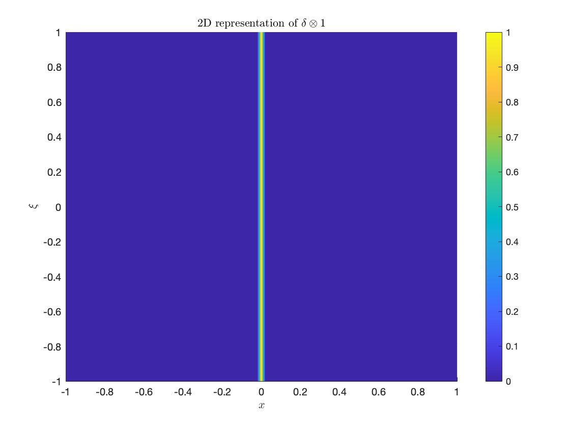
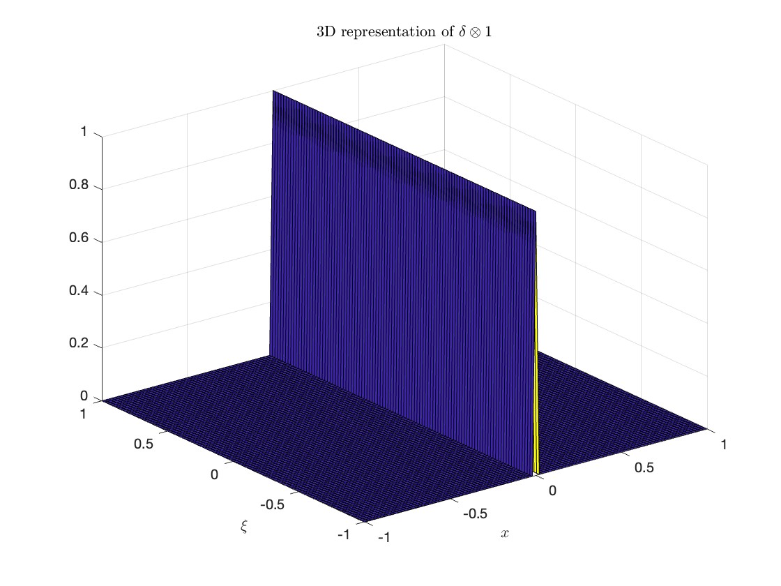
Figure 1. 2D and 3D representations of $\delta\otimes 1$.

From (39),

$$W\delta\ast W\varphi(x,\xi)=V_{\varphi}\delta(x,\xi)\overline{V_{\varphi}\delta(x,\xi)},$$

and

$$V_{\varphi}\delta(x,\xi)=\langle\delta,\pi(x,\xi)\varphi\rangle=\overline{\varphi(-x)}=\varphi(x)$$

so that

$$W\delta\ast W\varphi=(\delta\otimes 1)\ast W\varphi=2^{d/2}e^{-2\pi x^{2}}\int_{\mathbb{R}^{d}}e^{-2\pi\xi^{2}}d\xi=e^{-2\pi x^{2}}=|V_{\varphi}\delta|^{2},$$

as expected. Figure $2$ displays the time-frequency concentration of $\delta$.

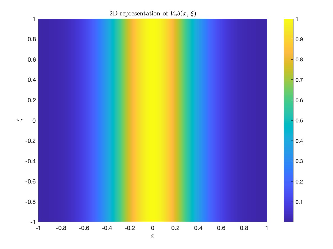
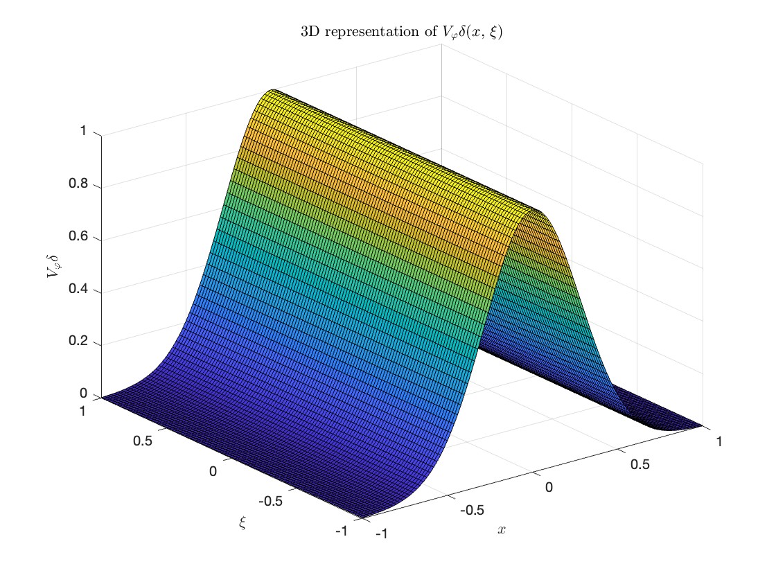
Figure 2. 2D and 3D representations of $V_{\varphi}\delta$.

Example 4.2 (The identity operator).

Consider $T=I$, the identity operator. Then

$$|\langle I\pi(z)g,\pi(w)g\rangle|=|V_{g}(\pi(z)g)(w)|=|V_{g}g(w-z)|\leq{C}\langle w-z\rangle^{-N},$$

for every $N\geq 0$, hence $I\in FIO_{\mathcal{G}}(I_{d\times d},N)$ ($I_{d\times d}$ being the identity matrix) for every $N\geq 0$. However, from (15),

$$W(If,Ig)(z)=W(f,g)(z)=\int_{{\mathbb{R}^{2d}}}T_{z}\delta(w)W(f,g)(w)dw$$

so that the Wigner kernel is the distribution $k(z,w)=\delta_{w-z}\in\mathcal{S}^{\prime}({\mathbb{R}^{2d}})$ which does not belong to any $FIO(I_{d\times d},N)$. In fact, $\bigcup_{\chi}FIO(\chi,N)$ is an algebra for $N>2d$, as proved in [6], but it is non-unital, whereas $\bigcup_{\chi}FIO_{\mathcal{G}}(\chi,N)$ is an algebra with identity, and Wiener property, see [8]. To be definite, let us test the validity of (37) for $g=\varphi$ as in (40). We have,

$$V_{\varphi}\varphi(x,\xi)=2^{-d/2}e^{-i\pi x\xi}e^{-\pi(x^{2}+\xi^{2})/2},\qquad x,\xi\in\mathbb{R}^{d},$$

hence:

$$|\langle I\pi(z)\varphi,\pi(w)\varphi\rangle|^{2}=2^{-d}e^{-\pi(z-w)^{2}},\qquad z,w\in{\mathbb{R}^{2d}}.$$

On the other hand,

$$[k\ast\Phi(w,z)] =\delta_{w-z}\ast\Phi$$

$$=\int_{\mathbb{R}^{4d}}\delta_{\vartheta-\zeta}\Phi(z-\zeta,w-\vartheta)d\theta d\zeta$$

$$=\int_{{\mathbb{R}^{2d}}}\Phi(z-\vartheta,w-\vartheta)d\theta$$

$$=\int_{{\mathbb{R}^{2d}}}\Phi(\lambda+\frac{1}{2}(z-w),\lambda-\frac{1}{2}(z-w))d\lambda,$$

where we used the change of variables $\vartheta=-\lambda+\frac{1}{2}(z+w)$. Since from (38)

$$\int_{{\mathbb{R}^{2d}}}\Phi(\lambda+\frac{1}{2}z,\lambda-\frac{1}{2}z)d\lambda=W\Phi(z,0)=2^{-d}e^{-\pi z^{2}},$$

we conclude:

$$[k\ast\Phi](w,z)=2^{-d}e^{-\pi(z-w)^{2}},$$

and (37) is satisfied. With respect to the off-diagonal variable $t=z-w\in{\mathbb{R}^{2d}}$, we may note a formal identity with the expressions in Example 4.1.

Example 4.3 (Metaplectic operators).

If $\mathcal{A}$ is a symplectic matrix on ${\mathbb{R}^{2d}}$, that is $\mathcal{A}^{T}J\mathcal{A}=J$, where

$$J=\begin{pmatrix}0_{d\times d}&I_{d\times d}\\ -I_{d\times d}&0_{d\times d}\end{pmatrix}$$

yields the standard symplectic form on ${\mathbb{R}^{2d}}$, the metaplectic operator $\hat{\mathcal{A}}$ is defined by the intertwining relation

$$\pi(\mathcal{A}z)=c_{\mathcal{A}}\hat{\mathcal{A}}\pi(z)\hat{\mathcal{A}}^{-1},\qquad z\in{\mathbb{R}^{2d}},$$

with a phase factor $c_{\mathcal{A}}\in\mathbb{C}$, $|c_{\mathcal{A}}|=1$. We denote by $Sp(d,\mathbb{R})$ the group of $2d\times 2d$ symplectic matrices and we refer to [13] and [14] for the theory of metaplectic operators. If $\mathcal{A}\in Sp(d,\mathbb{R})$ and $g\in\mathcal{S}(\mathbb{R}^{d})$, for every $N\geq 0$ there exists a $C_{N}>0$ such that:

(41) $$|\langle\hat{\mathcal{A}}\pi(z)g,\pi(w)g\rangle|\leq C_{N}\langle w-\mathcal{A}z\rangle^{-N},\qquad z,w\in{\mathbb{R}^{2d}},$$

see for example [9]. Hence, $\hat{\mathcal{A}}\in FIO_{\mathcal{G}}(\mathcal{A},N)$ for every $N$. Concerning the Wigner kernel, we note that:

$$W(\hat{\mathcal{A}}f)=Wf(\mathcal{A}^{-1}z)=\int_{{\mathbb{R}^{2d}}}\delta_{z=\mathcal{A}w}Wf(w)dw,$$

see for example [10, Proposition 1.3.7], hence the Wigner kernel of $\hat{\mathcal{A}}$ is given by:

$$k(z,w)=\delta_{z=\mathcal{A}w},$$

distribution density in $\mathcal{S}^{\prime}(\mathbb{R}^{4d})$. As in Example 4.2, pointwise estimates are not possible. By applying the smoothing in (37), we may recapture the Gabor matrix and the estimates (41).

Example 4.4.

A pseudodifferential operators $\sigma^{w}$ is defined as in (6). Its Wigner kernels is computed in [7, 4] and can be identified with the kernel $k(z,w)$ of a pseudodifferential operator with symbol in some class of distributions on $\mathbb{R}^{4d}$. By using Theorem 1.8 and, in particular, the smoothing (37), we may recapture the Gabor matrix and the results of [15, 16], i.e., $\sigma^{w}\in FIO_{\mathcal{G}}(I_{d\times d},N)$.

Example 4.5 (Generalized metaplectic operators).

Generalized metaplectic operators can be defined as products:

$$M_{\sigma,\mathcal{A}}=\sigma^{w}\hat{\mathcal{A}},$$

with $\sigma^{w}$ as in Example 4.4 and $\hat{\mathcal{A}}$ as in Example 4.3. Under suitable assumptions on $\mathcal{A}$, $M_{\sigma,\mathcal{A}}$ can be written as a FIO of type I, as in (10), with quadratic phase function and associated linear canonical transformation $\chi=\mathcal{A}$. The Wigner kernel of $M_{\sigma,\mathcal{A}}$ is given by $k(z,w)=h(z,\mathcal{A}w)$, where $h$ is the Wigner kernel of $\sigma^{w}$. Again, by (37), we may recapture the Gabor matrix and prove that $M_{\sigma,\mathcal{A}}\in FIO_{\mathcal{G}}(\mathcal{A},N)$. At the moment, the characterization of the Wigner kernel for a FIO of type I with general nonlinear canonical transformation $\chi$ is still an open problem.

References

- [1] R. Beals. Characterization of pseudodifferential operators and applications. Duke Math. J., 44(1):45–57, 1977.
- [2] A. Bényi and K.A. Okoudjou. Modulation Spaces With Applications to Pseudodifferential Operators and Nonlinear Schrödinger Equations, Springer New York, 2020.
- [3] P. Boggiatto, G. De Donno and A. Oliaro. A class of quadratic time-frequency representations based on the short-time Fourier transform. Operator Theory: Advances and Appl., 172: 235–249, 2006.
- [4] E. Cordero, G. Giacchi and L. Rodino. Wigner Analysis of Operators. Part II: Schrödinger equations. Commun. Math. Phys., to appear. arXiv:2208.00505
- [5] E. Cordero, G. Giacchi and L. Rodino. Wigner Representation of Schrödinger Propagators. Submitted. arXiv:2311.18383v2
- [6] E. Cordero, G. Giacchi, L. Rodino, and M. Valenzano. Wigner Analysis of Fourier Integral Operators with symbols in the Shubin classes. Submitted. arXiv:2402.02809
- [7] E. Cordero and N. Rodino. Wigner Analysis of Operators. Part I: Pseudodifferential Operators and Wave Front Sets. Appl. Comput. Harmon. Anal. 58 (2022) 85-123.
- [8] E. Cordero, K. Gröchenig, F. Nicola and L. Rodino. Wiener algebras of Fourier integral operators. J. Math. Pures Appl. (9), 99(2):219–233, 2013
- [9] E. Cordero, K. Gröchenig, F. Nicola and L. Rodino. Generalized Metaplectic Operators and the Schrödinger Equation with a Potential in the Sjöstrand Class, J. Math. Phys., 55(8):081506, 17, 2014
- [10] E. Cordero and L. Rodino, Time-Frequency Analysis of Operators, De Gruyter Studies in Mathematics, 2020.
- [11] N.C. Dias, M. de Gosson, and J.N. Prata. A metaplectic perspective of uncertainty principles in the Linear Canonical Transform domain. Submitted.
- [12] H. G. Feichtinger, Modulation spaces on locally compact abelian groups, Technical Report, University Vienna, 1983, and also in Wavelets and Their Applications, M. Krishna, R. Radha, S. Thangavelu, editors, Allied Publishers, 99–140, 2003.
- [13] M. de Gosson. The Wigner Transform. World Scientific Pub Co Inc, 2017.
- [14] K. Gröchenig. Foundations of time-frequency analysis. Birkhäuser Boston, Inc., Boston, MA, 2001.
- [15] K. Gröchenig. Time-Frequency Analysis of Sjöstrand’s Class. Rev. Mat. Iberoamericana, 22(2):703–724, 2006.
- [16] K. Gröchenig and Z. Rzeszotnik. Banach algebras of pseudodifferential operators and their almost diagonalization. Ann. Inst. Fourier. 58(7):2279-2314, 2008.
- [17] L. Hörmander. Fourier integral operators I. Acta Math., 127:79–183, 1971.
- [18] H. Knutsen. Notes on Hardy’s uncertainty principle for the Wigner distribution and Schrödinger evolutions Journal of Mathematical Analysis and Applications, 525(1):127116, 2023.
- [19] E. Wigner. On the Quantum Correction for Thermodynamic Equilibrium. Phys. Rev., 40(5):749-759, 1932.