Realization of two-qubit gates and multi-body entanglement states in an asymmetric superconducting circuits
Abstract
In recent years, the tunable coupling scheme has become the mainstream scheme for designing superconducting quantum circuits. By working in the dispersive regime, the ZZ coupling and high-energy level leakage can be effectively suppressed and realize a high fidelity quantum gate. We propose a tunable fluxonium-transmon-transmon (FTT) coupling scheme. In our system, the coupler is a frequency tunable transmon qubit. Both qubits and coupler are capacitively coupled. The asymmetric structure composed of fluxonium and transmon will optimize the frequency space and form a high fidelity two-qubit quantum gate. By decoupling, the effective coupling strength can be easily adjusted to close to the net coupling between qubits. We numerical simulation the master equation to reduce the quantum noise to zero. We study the performance of this scheme by simulating the general single-qubit gate and two-qubit gate. In the bias point of the qubits, we achieve a single qubit gate with 99.99 fidelity and a two-qubit gate with 99.95 fidelity. By adjusting the nonlinear Kerr coefficient of fluxonium to an appropriate value, we can achieve a multi-body entanglement state. We consider the correlation between the two qubits and the coupler, and the magnetic flux passing through one qubit has an effect on the other qubit and the coupler. Finally, we analyze the quantum correlation of the two-body entanglement state.
I INTRODUCTION
Quantum superconducting circuits based on transmon have become a mainstream trend over the years Majer et al. (2007); DiCarlo et al. (2009); Zeytinoğlu et al. (2015); Egger et al. (2019); Krinner et al. (2020), because of transmon’s unique circuit structure Koch et al. (2007), the charge dispersion is small and insensitive to the charge noise. At the same time, transmon can maintains a good non-harmonic so that the operation can be accurately addressed. However, a high fidelity quantum gates require coherent qubits and suitable qubit-qubit coupling Preskill (2018). As the circuit structure becomes more and more complex, unnecessary qubit interactions will degrade gate performance. A coupling transmon can deal with unnecessary coupling and frequency congestion McKay et al. (2016); Mundada et al. (2019); Li et al. (2020); Han et al. (2020); Xu et al. (2020).The effective coupling between two qubits can be controlled by adjusting the intermediate-mediated coupler frequency. The coupling strength is set to zero when we running a single qubit gate, and the coupling between qubits can be turned on when we running a double qubit gate.
The selection of fluxonium as a qubit for superconducting quantum circuits is a promising improvement Xiang et al. (2013); Arute et al. (2019); Place et al. (2021); Jurcevic et al. (2021). Fluxonium can prevents charge and flux-induced dephase by shunting the Josephson junction and a large linear inductor Bao et al. (2022), while retaining a large an-harmonies. Furthermore, in order to achieve a considerable coherence time Nguyen et al. (2019), the fluxonium needs to work at a much lower frequency than that of the transmon. The energy relaxation can be suppressed at a low qubit frequency, which means a reduction in the two-qubit gate velocity limited by the directly qubit-qubit coupling strength. Fluxonium has been used in tunable coupling systems Moskalenko et al. (2021), enabling flux quantum circuits with additional modes via capacitive coupling of quantum bits and couplers.
Imperfect two-qubit gate operation is an urgent problem in superconducting quantum circuits. In order to improve the fidelity of quantum gates, different experiments research groups choose different types of qubits or coupler. Neill et al. achieved a high coherence and fast tunable coupling by using Xmon qubits Chen et al. (2014), and a two-qubit idle gate with 99.56 fidelity. Hayato et al. implemented a high-performance two-qubit parametric gate based on double-transmon couplers Kubo and Goto (2023). Although the fidelity is high enough, the detuning between qubits is not large enough and the qubit frequency is high. Therefore, in order to improve the detuning between qubits and make the system work in dispersive regime, we choose fluxonium as a qubit to couple with transmon, which can alleviate the problem of frequency-crowding Hertzberg et al. (2020).
In this work, in order to solve the problem of frequency-crowding and form a stable and reliable quantum gate, we propose a fluxonium and transmon systems with tunable coupler capacitance coupling(FTT), which can achieve a high fidelity two-qubit gates. By adjusting the frequency of the coupler and changing the effective coupling strength between the two qubits, the net coupling can be effectively closed. At this time, we can simulate a single-qubit gate in our system without interference from other qubits. Two-qubit gates operate in the dispersive regime can suppress leakage of higher excited states. In this way, the coherence time of two qubits and the fidelity of the system can be improved. We can simulate their relaxation time and dephasing time in scqubits, and compare the relationship between the coherence time and the gate time. In addition, we use an asymmetric structure, and realize the preparation of entanglement states and analyze the quantum correlation of the two-body entanglement states based on the nonlinear Kerr coefficient of fluxonium.
II The Theoretical Model
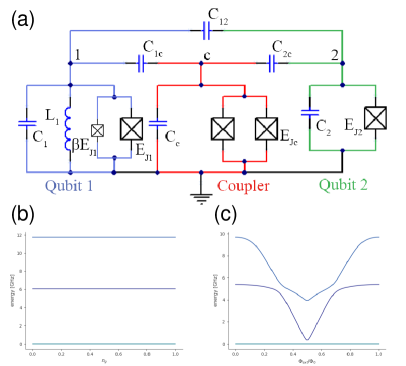
We use a nonlinear fluxonium qubit and a transmon qubit, which are capacitively coupled to a grounded transmon coupler, as shown in Fig. 1(a). The tunable coupler consists of a transmon with an tunable frequency, and there is a direct capacitive coupling between the fluxonium and transmon qubits, the direct coupling between two qubits is much weaker. We use a Josephson loop (superconducting quantum interference device) instead of the Josephson junction in fluxonium, which can produce nonlinear effect and the frequency of transmon is fixed. When we only consider the qubits model and the capacitance coupling between them, the Hamiltonian of our system is (see Appendix A)
| (1) |
where , , and represent the charging, Josephson, and inductive energies, respectively. The ratio of Josephson energy of the small and big junction is =0.1. Subscripts index the fluxonium nodes and the transmon nodes, respectively, and subscript labels the coupler node. The coupling strength (i,j 1,2,c) represents the coupling strength between different modes, and the direct coupling strength is far less than the indirect coupling strength and .
In our numerical simulation, the Fluxonium and transmon are used at the zero flux bias point (/) and the charge bias point (), respectively, as shown in Fig. 1(b) and Fig. 1(c). The external magnetic flux can be applied to the Josephson junction loop in the coupler through the magnetic flux-bias line, thus wen can change the frequency of the tunable coupler. The transmon with charging energy and inductance energy , the transmon needs to work under the limit of . The fluxonium is very sensitive to the external magnetic flux, when we simulate a two-qubit gate, we set the external flux to zero. When we adjust the nonlinear Kerr coefficient, we need to turn on it.
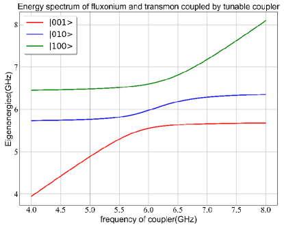
We describe the quantum state by using the notation , where , , and denote the energy eigen-states in the uncoupled basis of fluxonium, the coupler, and transmon, respectively. We need to avoid crossing between computational state and , we also need to avoid crossing between computational state and . The size is twice the corresponding coupling strength as shown in Fig. 2.
The circuit parameters and the corresponding coupling strength are used in our numerical simulation as shown in Table 1. The qubit and coupler are detuned and the coupling is dispersive. The coupling of two qubits has two channels, in which direct coupling through capacitance and indirect coupling through coupler. The coupler decouple by the Schrieffer-Wolff transformation(SWT)Yan et al. (2018). Finally, the effective Hamiltonian of two qubits can be obtained (see Appendix B):
| (2) |
where and are the frequencies of fluxonium and transmon, respectively. is the nonlinear Kerr coefficient of fluxonium. is the anharmonicity of transmon, and is the effective coupling strength between fluxonium and transmon. corresponds to the generation (annihilation) operator of the corresponding mode.
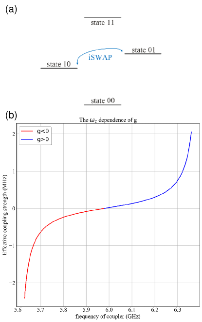
In Fig. 3(a), we preset the energy level diagram of the tunable coupling system and the range of transitions. Through the gate, we can realize the transition of . By applying microwave pulses to different qubits, we can realize the transition from state to state or state .
| Fluxonium | 0.9 | 1.0 | 4.5 | 5.7 |
| transmon | 0.32 | 16.0 | 6.4 | |
| coupler | 0.32 | 12.8 | ||
| coupling strength | 242.9 | 307.11 | 34.7 | |
The effective coupling strength depends on the frequency of the coupler, as shown in Fig. 3(b). We choose the coupler frequency from 4.0 to 8.0 corresponds to the adjustment range of the tunable coupler.
When the coupler frequency reaches to 5.97, the net coupling between qubits need to completely turn off. When the whole system works at the coupling zero point, we apply microwave drive the state of a single qubit rotate accordingly without affect the state of another qubit. When we operate the two-qubit gates, we can open the interaction and realize the controllable gate operation. We can also change the frequency of the coupler by applying the magnetic flux pulse, so as to achieve the effect of changing the effective coupling strength.
The operation of quantum gates can produce leakage stateChu and Yan (2021), the most important is the unnecessary excitation of the coupler, which makes the whole system transition to a non-computational state, and forming a gate error. We operate the coupler in the dispersion regime to perform the two-qubit gate operation, which strongly inhibits the leakage of the coupler to the excited state. In the dispersion limit, the frequency difference between the coupler and the qubit is much larger than the coupling strength .
III GATE PRINCIPLES
III.1 Single-qubit gates
We simulate the quantum gates with QuTip in PYTHONJohansson, Nation, and Nori (2012). First, we set the effective coupling is zero and close the net coupling of two qubits. At this time, a flux pulse passing through the flux bias line. After turning off the coupling between two qubits, a microwave drive with the frequency of single qubit. The drive time of microwave determines the rotation angle of the quantum state on the Bloch sphere. Taking the rotating wave approximation, the driving Hamiltonian can be written asKrantz et al. (2019)
| (3) |
Where is a dimensionless parameter determined by circuit parameters and is a dimensionless envelope function. In addition, is the voltage amplitude, and are the Pauli matrices in the and directions, respectively. The in-phase component and the out-of-phase component can control the axis of rotation. When , the rotation revolves around the -axis, and when , the rotation revolves around the -axis. We numerically simulate the gate, whose matrix expression is
| (4) |
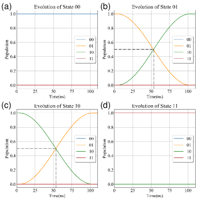
We simulate the gate on fluxonium by using modulated Gaussian pulses (with "mesolve" in QuTip). By applying a microwave pulse to realize a single-qubit gate, we simulate the evolution of the system state under four different initial states. The evolution of each state under different initial states are shown in Fig. 4.
We simulate the evolution of quantum states with an initial state of and , respectively. We set the modulate pulse frequency as the frequency of fluxonium GHz and the gate time as . From the figure, we can see that and , which is consistent with the fidelity theoretical result. Due to the pulse acting on fluxonium, the quantum state of transmon remains unchanged.
| (5) |
Finally, we use fidelity to calculate the proximity between actual quantum state and ideal quantum state . The fidelity of the single-qubit gate is 99.99, and the error occurs after six decimal places.
Thus, we obtain a single-qubit gate with high fidelity by modulating the pulse waveform. If it is necessary to obtain a state with a better fidelity, which may be necessary to optimize the pulse waveform to further suppress the leakage of excited states.
III.2 Two-qubit gates
Next, we implement a universal two-qubit gate via an effective Hamiltonian, and only consider the first two energy levels of the qubits. When fluxonium and transmon are in resonance and the two qubits are truncated to two enegry levels, by the rotating wave approximation, the Hamiltonian between qubits approximates to
| (6) |
The unitary corresponding to the qubit-qubit interaction is
| (7) |
When two qubits are in resonance and the gate time , we can get the matrix expression of gate:
| (8) |
Therefore, we can use the pulse sequence to realize the gate: (1)an error type square wave acting on fluxonium or transmon to make up the frequency difference between two qubits, in order to reaches to the resonance state. (2)A rectangular magnetic flux pulse acting on the coupler will changes the frequency of the coupler so that the effective coupling strength reaches to the gate operating point. The time length of the two pulses is , which can make the gate operate completely and prevent the leakage of other quantum states.
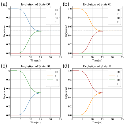
By applying a magnetic flux pulse and a rectangular pulse to realize the two-qubit gate, we simulate the evolution of system states under six different initial states. We simulate the gates with QuTip in PYTHON. The evolution of each state under different initial states as shown in Fig. 5. We simulate the evolution of quantum states with an initial state of and , respectively. In this case, the total qubit-qubit coupling is 250 and the coupler frequency is tuned to 4.27. We can see that and , which is consistent with the fidelity theoretical results. After exchanging the states of two qubits will result in a global phase of . When the initial state is at or , it is a horizontal straight line. We get the fidelity of the two quantum states is 99.97.
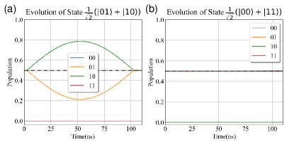
In order to show the quantum evolution of some special initial states, we select the evolution of two Bell States under the gate, as shown in Fig. 6. The quantum state with an initial state of exchanges internally under the action of the gate and finally returns to the initial state, there is an additional global phase. However, the quantum state with initial state does not change ecologically through the action of gate, there are two straight lines. We finally get the result of 97.63. A gate operation can be completed within the coherence time of two qubits.
| coherence time | dephase time | |
|---|---|---|
| Fluxonium | 309.42 | 56.7 |
| transmon | 260.82 | 506.99 |
| single-qubit gate | two-qubit gate | |
| gate time | 15 | 103 |
Depending on the physical structure of fluxonium, capacitance and inductance are introduced into charge and inductor noise channels, respectively. Because of the SQUID in fluxonium, we also take into account the flux bias channel connected to it, as well as the quasi-particle noise introduced by the Josephson junction. Whereas, for a fixed-frequency transmon, we only consider the charge noise caused by its capacitance.
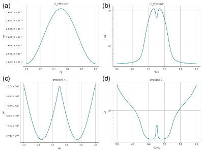
Here we use Python’s scqubitsGroszkowski and Koch (2021) package to simulate the three energy levels and coherence time of two qubits. The qubit parameters used in our simulation are shown in Table 1. For transmon, the offset charge we selected from 0 to 1; For fluxonium, we choose the external magnetic flux from 0 to . When two qubits work at the bias point, the frequency of fluxonium is , and the frequency of transmon is . From Fig. 7, we can get the effective coherence time of fluxonium is 309.42 , and the effective coherence time of the transmon is 260.82 . In addition, the effective dephase time of fluxonium is 56.7 , and the effective dephase time of transmon is 506.99 . The operation time of single-qubit gate and two-qubit gate is 15 and 103 , respectively. Therefore, from the perspective of theoretical calculation, we can complete the whole gate operation in the finite qubit coherence time.
IV Preparation of Schrödinger Cat states
We can prepare the non-classical quantum states by using Kerr non-linearity effect, we need to take into account the nonlinear effects of the fluxonium. First, fluxonium can prepare the coherent state by using the coherent pulses. The coherent state will evolve with the Kerr non-linearity effects. Then, after the displacement pulse , the Kerr non-linearity can be adjusted by using the fluxonium SQUID’s magnetic flux bias pulse. Under the influence of the nonlinear Hamiltonian, the rotating speed of the coherent state in the phase space is not uniform, so the kerr Cat state can be produced at the right time. The evolution of a qubit with the initial state under Kerr non-linearity effect can be written as He et al. (2023)
| (9) |
The coherent state is expanded into a Fock state for reforming calculation, and when is at a certain value, the final state will evolve into a multi-body Cat state Tan, Zhao, and Guo (2023); Zhao, Guo, and Tan (2019, 2020). In the calculation, the relationship between Kerr non-linearity and time that separates the real part from the imaginary part is and . In particular, when , the final state is
| (10) |
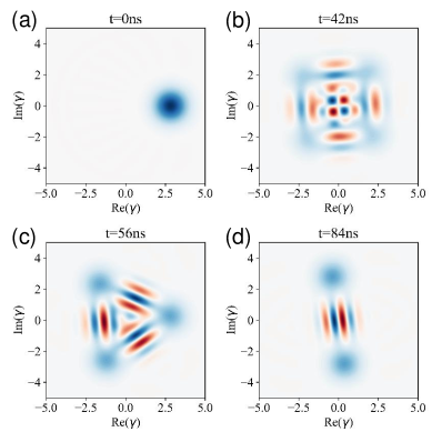
In our simulation, the flux bias pulse in the coupler is turned off at this point so that transmon and fluxonium can interact with each other. Wigner tomography can accomplish by applying a qubit to drive the transmon and a readout pulse to drive the readout resonator. The pulse sequence of the Kerr Cat state as shown in Appendix C. We chose =2 to simulate the evolution of the coherent state to the two-body Cat state. We use a non-linear Kerr Hamiltonian to simulate the generation of Cat states. The flux bias pulse in SQUID sets the Kerr non-linearity coefficient to , the corresponding evolution time is . When the widths of the flux bias pulses are , , and , respectively, we achieve the two-, three-, and four-body Cat states, and the numerical simulation results of the Wigner tomography are shown in Fig. 8.
In addition, we also calculate the quantum correlation of the two-body Cat states with different photon numbers , where . The quantum correlation of multi-body Cat state can be written as
| (11) |
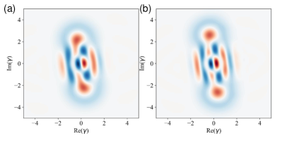
Where is the Wigner function when multi-body Cat state at , and is the number of photons. The quantum systems with different photon numbers can be obtained by varying the displacement of the pump pulse. As shown in Fig. 9, figure 9 (a) is the two-body Cat state correlation when and , and figure 9 (b) is the two-body Cat state correlation when and . The quantum correlation of the two-body Cat state is similar to the shape of the Cat state, but it shows the characteristics of layer upon layer of nesting.
V CONCLUSION
In conclusion, we propose a tunable coupling scheme based on fluxonium-transmon-transmon (FTT), which is used to realize a high fidelity two-qubit gates with fixed frequency fluxonium and transmon. In this system, both qubits and coupler are capacitively coupled, and the coupler is a frequency tunable transmon qubit. By decoupling the coupler from the system, the effective coupling strength can be easily adjusted to zero to close the net coupling between qubits. We study the performance of this scheme by simulating the general single-qubit gate and two-qubit gate. We simulate single-qubit gates and two-qubit gates (iSWAP) on circuits with FTT structures, respectively. Single-qubit gates can achieve 99.99 fidelity within . Without decoherence, two-qubit gates can achieve 99.95 fidelity within .
FTT structure is a feasible scheme in quantum circuit structure. By selecting appropriate circuit devices to form the qubit frequency and the coupling strength, which can operate the quantum gate. The capacitive coupling of different types of superconducting qubits can provide a new approach for achieving scalable and large-scale superconducting quantum processors. This asymmetric structure not only generates high-fidelity two-qubit gates, but also generates Schrödinger Cat states in fluxonium. By adjusting the nonlinear Kerr coefficient of fluxonium, the multi-body Schrödinger Cat state can be obtained in Wigner tomography. Compared with ordinary superconducting circuits, we consider the nonlinear Kerr effect of fluxonium and realize the Cat states, and analyze the quantum correlation of two-body Cat states. Our simulation shows that the energy level gap between fluxonium at and transmon at is very loose, but the coupling still stable, which is very effective for multi-level structures. Our method can effectively solve the problem of frequency-crowding and form a high fidelity quantum gate, at the same time produce a Schrödinger Cat state in the qubits.
VI Acknowledgement
Financial support from the project funded by the State Key Laboratory of Quantum Optics and Quantum Optics Devices, Shanxi University, Shanxi, China (Grants No.KF202004 and No.KF202205).
Appendix A Circuit Hamiltonian And Quantization
The circuit diagram for realizing our adjustable coupling scheme as shown in Fig. 1(a), which contains two qubits: qubit 1 (blue) and qubit 2 (green) and a coupler (red). Qubit1 is a fixed frequency fluxonium, qubit2 is a fixed frequency transmon, and the coupler is a frequency adjustable transmon. Low frequency fluxonium consists of a capacitor, an inductor and a Josephson junction.
We choose the flux node corresponds to node in the graph as the generalized coordinates of the system. We can write out the Lagrange function of the circuit by using the flux node :
| (12) |
| (13) |
| (14) |
Where is the flux quantum. Writing out the kinetic energy part in matrix form:
| (15) |
The capacitance matrix is:
| (16) |
The inverse capacitance matrix is:
| (17) |
The Hamiltonian of the system can be obtained:
| (18) |
By using the canonical quantization, the quantized Hamiltonian can be rewritten as
| (19) |
Where is the parameter factor, is the Cooper pair number operator, is the inductance energy of the corresponding mode and is the charging energy of the corresponding mode.
In the fluxonium and transmon coupling regime, we substitute the creation (annihilation) operator into the Hamiltonian
| (20) |
| (21) |
The Hamiltonian of the system becomes ():
| (22) |
| (23) |
| (24) |
| (25) |
| (26) |
Where corresponds to the creation (annihilation) operator of the corresponding mode, Taylor coefficient , is the coupling strength of the three(four)-wave mixing,
| (27) |
| (28) |
We approximate looks fluxonium as a harmonic oscillator, the nonlinear kerr coefficient can be calculated as the dispersion of the transition frequencies between the neighboring energy levels,
| (29) |
The coupling strength is
| (30) |
| (31) |
is the coupling strength of qubit-coupler, and is the coupling strength of qubit-qubit. The equation not only retains the interaction term, but also retains the conter-rotating term. The contribution of double excitation interaction is also significant in the dispersion regime where the coupler frequency is much greater than that of the qubit frequency.
Appendix B Schrieffer-Wolff Transformation
In order to decouple, we apply the Schrieffer-Wolff transformation
| (32) |
Where , we expand in the second order. We finally obtain the effectively Hamiltonian:
| (33) |
where
| (34) |
| (35) |
| (36) |
| (37) |
| (38) |
Appendix C Pulse Sequence
The pulse sequence used for quantum gate operation as shown in Fig. 10, and the pulse sequence used in entanglement state generation and numerical simulation as shown in Fig. 11.
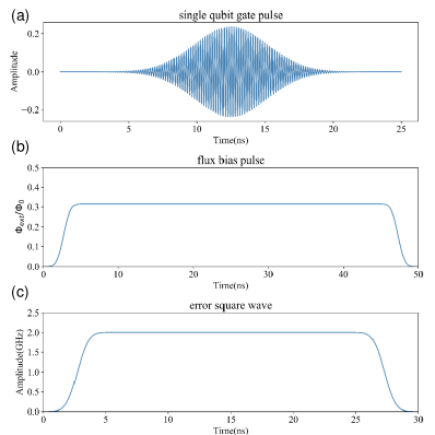
A single-qubit gate pulse consists of a microwave source provide a stable drive pulse. An arbitrary wave generator (AWG) provide a base-band pulse. The frequency of the driving pulse is , and the envelope of the base-band pulse is , and the frequency is . The IQ-mixer combines the two signals to produce a new signal with a waveform of and a frequency .
The rectangular flux pulse passing through the flux bias line to the coupler’s Josephson junction loop with a magnitude of a multiple of the superconducting flux quantum . During the flux bias, the effective coupling strength can be adjusted to a suitable frequency.
Error type square waves acts on the qubits through an XY line, the amplitude of which is the energy level difference between the two qubits. The effect is to compensate for the energy level difference between the qubits, so that the two qubits can reach a resonance state. During the pulse, the two-qubit gate works normally.
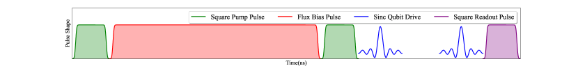
In Fig. 11, the first green pulse is a square pump pulse acts on fluxonium, which causes a displacement make the vacuum state becomes coherent state .
The first red pulse is the flux bias pulse acts on SQUID in fluxonium, which can adjust the nonlinear Kerr coefficient to an appropriate strength, and the duration of the pulse can be determined by the nonlinear Kerr coefficient, and the Kerr Cat state generated in fluxonium under the evolution of nonlinear Hamiltonian.
The next four pulses together form the pulse sequence of the Wigner tomography. The second green pulse brings a displacement . Here, we apply two pulses (blue pulse) into transmon. Using the time interval between the two pulses, this sequence can be considered as a parity measurement, where the state of transmon corresponds to the measurement probability . Considering the frequency shift of transmon, we employ a function of to cover a larger spectrum range uniformly. The state of transmon can be measured by the final readout pulse (the purple pulse) applied to a readout resonator capacitively coupled to transmon.
References
- Majer et al. (2007) J. Majer, J. Chow, J. Gambetta, J. Koch, B. Johnson, J. Schreier, L. Frunzio, D. Schuster, A. A. Houck, A. Wallraff, et al., “Coupling superconducting qubits via a cavity bus,” Nature 449, 443–447 (2007).
- DiCarlo et al. (2009) L. DiCarlo, J. M. Chow, J. M. Gambetta, L. S. Bishop, B. R. Johnson, D. Schuster, J. Majer, A. Blais, L. Frunzio, S. Girvin, et al., “Demonstration of two-qubit algorithms with a superconducting quantum processor,” Nature 460, 240–244 (2009).
- Zeytinoğlu et al. (2015) S. Zeytinoğlu, M. Pechal, S. Berger, A. Abdumalikov Jr, A. Wallraff, and S. Filipp, “Microwave-induced amplitude-and phase-tunable qubit-resonator coupling in circuit quantum electrodynamics,” Physical Review A 91, 043846 (2015).
- Egger et al. (2019) D. J. Egger, M. Ganzhorn, G. Salis, A. Fuhrer, P. Mueller, P. K. Barkoutsos, N. Moll, I. Tavernelli, and S. Filipp, “Entanglement generation in superconducting qubits using holonomic operations,” Physical Review Applied 11, 014017 (2019).
- Krinner et al. (2020) S. Krinner, P. Kurpiers, B. Royer, P. Magnard, I. Tsitsilin, J.-C. Besse, A. Remm, A. Blais, and A. Wallraff, “Demonstration of an all-microwave controlled-phase gate between far-detuned qubits,” Physical Review Applied 14, 044039 (2020).
- Koch et al. (2007) J. Koch, M. Y. Terri, J. Gambetta, A. A. Houck, D. I. Schuster, J. Majer, A. Blais, M. H. Devoret, S. M. Girvin, and R. J. Schoelkopf, “Charge-insensitive qubit design derived from the cooper pair box,” Physical Review A 76, 042319 (2007).
- Preskill (2018) J. Preskill, “Quantum computing in the nisq era and beyond,” Quantum 2, 79 (2018).
- McKay et al. (2016) D. C. McKay, S. Filipp, A. Mezzacapo, E. Magesan, J. M. Chow, and J. M. Gambetta, “Universal gate for fixed-frequency qubits via a tunable bus,” Physical Review Applied 6, 064007 (2016).
- Mundada et al. (2019) P. Mundada, G. Zhang, T. Hazard, and A. Houck, “Suppression of qubit crosstalk in a tunable coupling superconducting circuit,” Physical Review Applied 12, 054023 (2019).
- Li et al. (2020) X. Li, T. Cai, H. Yan, Z. Wang, X. Pan, Y. Ma, W. Cai, J. Han, Z. Hua, X. Han, et al., “Tunable coupler for realizing a controlled-phase gate with dynamically decoupled regime in a superconducting circuit,” Physical Review Applied 14, 024070 (2020).
- Han et al. (2020) X. Han, T. Cai, X. Li, Y. Wu, Y. Ma, Y. Ma, J. Wang, H. Zhang, Y. Song, and L. Duan, “Error analysis in suppression of unwanted qubit interactions for a parametric gate in a tunable superconducting circuit,” Physical Review A 102, 022619 (2020).
- Xu et al. (2020) Y. Xu, J. Chu, J. Yuan, J. Qiu, Y. Zhou, L. Zhang, X. Tan, Y. Yu, S. Liu, J. Li, et al., “High-fidelity, high-scalability two-qubit gate scheme for superconducting qubits,” Physical Review Letters 125, 240503 (2020).
- Xiang et al. (2013) Z.-L. Xiang, S. Ashhab, J. You, and F. Nori, “Hybrid quantum circuits: Superconducting circuits interacting with other quantum systems,” Reviews of Modern Physics 85, 623 (2013).
- Arute et al. (2019) F. Arute, K. Arya, R. Babbush, D. Bacon, J. C. Bardin, R. Barends, R. Biswas, S. Boixo, F. G. Brandao, D. A. Buell, et al., “Quantum supremacy using a programmable superconducting processor,” Nature 574, 505–510 (2019).
- Place et al. (2021) A. P. Place, L. V. Rodgers, P. Mundada, B. M. Smitham, M. Fitzpatrick, Z. Leng, A. Premkumar, J. Bryon, A. Vrajitoarea, S. Sussman, et al., “New material platform for superconducting transmon qubits with coherence times exceeding 0.3 milliseconds,” Nature communications 12, 1779 (2021).
- Jurcevic et al. (2021) P. Jurcevic, A. Javadi-Abhari, L. S. Bishop, I. Lauer, D. F. Bogorin, M. Brink, L. Capelluto, O. Günlük, T. Itoko, N. Kanazawa, et al., “Demonstration of quantum volume 64 on a superconducting quantum computing system,” Quantum Science and Technology 6, 025020 (2021).
- Bao et al. (2022) F. Bao, H. Deng, D. Ding, R. Gao, X. Gao, C. Huang, X. Jiang, H.-S. Ku, Z. Li, X. Ma, et al., “Fluxonium: an alternative qubit platform for high-fidelity operations,” Physical Review Letters 129, 010502 (2022).
- Nguyen et al. (2019) L. B. Nguyen, Y.-H. Lin, A. Somoroff, R. Mencia, N. Grabon, and V. E. Manucharyan, “High-coherence fluxonium qubit,” Physical Review X 9, 041041 (2019).
- Moskalenko et al. (2021) I. Moskalenko, I. Besedin, I. Simakov, and A. Ustinov, “Tunable coupling scheme for implementing two-qubit gates on fluxonium qubits,” Applied Physics Letters 119 (2021).
- Chen et al. (2014) Y. Chen, C. Neill, P. Roushan, N. Leung, M. Fang, R. Barends, J. Kelly, B. Campbell, Z. Chen, B. Chiaro, et al., “Qubit architecture with high coherence and fast tunable coupling,” Physical review letters 113, 220502 (2014).
- Kubo and Goto (2023) K. Kubo and H. Goto, “Fast parametric two-qubit gate for highly detuned fixed-frequency superconducting qubits using a double-transmon coupler,” Applied Physics Letters 122 (2023).
- Hertzberg et al. (2020) J. Hertzberg, S. Rosenblatt, J. Chavez, E. Magesan, J. Smolin, J.-B. Yau, V. Adiga, M. Brink, E. Zhang, J. Orcutt, et al., “Effects of qubit frequency crowding on scalable quantum processors,” Bulletin of the American Physical Society 65 (2020).
- Yan et al. (2018) F. Yan, P. Krantz, Y. Sung, M. Kjaergaard, D. L. Campbell, T. P. Orlando, S. Gustavsson, and W. D. Oliver, “Tunable coupling scheme for implementing high-fidelity two-qubit gates,” Physical Review Applied 10, 054062 (2018).
- Chu and Yan (2021) J. Chu and F. Yan, “Coupler-assisted controlled-phase gate with enhanced adiabaticity,” Physical Review Applied 16, 054020 (2021).
- Johansson, Nation, and Nori (2012) J. R. Johansson, P. D. Nation, and F. Nori, “Qutip: An open-source python framework for the dynamics of open quantum systems,” Computer Physics Communications 183, 1760–1772 (2012).
- Krantz et al. (2019) P. Krantz, M. Kjaergaard, F. Yan, T. P. Orlando, S. Gustavsson, and W. D. Oliver, “A quantum engineer’s guide to superconducting qubits,” Applied physics reviews 6 (2019).
- Groszkowski and Koch (2021) P. Groszkowski and J. Koch, “Scqubits: a python package for superconducting qubits,” Quantum 5, 583 (2021).
- He et al. (2023) X. He, Y. Lu, D. Bao, H. Xue, W. Jiang, Z. Wang, A. Roudsari, P. Delsing, J. Tsai, and Z. Lin, “Fast generation of schrödinger cat states using a kerr-tunable superconducting resonator,” Nature communications 14, 6358 (2023).
- Tan, Zhao, and Guo (2023) W.-H. Tan, C.-Y. Zhao, and Q.-Z. Guo, “Entanglement criterion of n qubit system br,” ACTA PHYSICA SINICA 72 (2023).
- Zhao, Guo, and Tan (2019) C.-Y. Zhao, Q.-Z. Guo, and W.-H. Tan, “A simple entanglement criterion of two-qubit system,” International Journal of Modern Physics B 33, 1950197 (2019).
- Zhao, Guo, and Tan (2020) C.-Y. Zhao, Q.-Z. Guo, and W.-H. Tan, “A novel entanglement criterion of two-qubit system,” International Journal of Modern Physics B 34, 2050022 (2020).
- Shore and Knight (1993) B. W. Shore and P. L. Knight, “The jaynes-cummings model,” Journal of Modern Optics 40, 1195–1238 (1993).