Exponentially Weighted Moving Models

Abstract

An exponentially weighted moving model (EWMM) for a vector time series fits a new data model each time period, based on an exponentially fading loss function on past observed data. The well known and widely used exponentially weighted moving average (EWMA) is a special case that estimates the mean using a square loss function. For quadratic loss functions EWMMs can be fit using a simple recursion that updates the parameters of a quadratic function. For other loss functions, the entire past history must be stored, and the fitting problem grows in size as time increases. We propose a general method for computing an approximation of EWMM, which requires storing only a window of a fixed number of past samples, and uses an additional quadratic term to approximate the loss associated with the data before the window. This approximate EWMM relies on convex optimization, and solves problems that do not grow with time. We compare the estimates produced by our approximation with the estimates from the exact EWMM method.

1 Introduction

We consider the problem of fitting a time-varying model to a vector time series, updating it each time period as new data is observed. Assuming that recent data is more relevant than data from many periods in the past, the model is fit giving more weight to recent past values and lower weight to values far in the past.

Rolling window model.

One simple method to do this is to fit the model at time period $t$ using a rolling window of $R$ previous values of the time series. The choice of $R$ involves a trade-off. When it is small, we have fewer data to fit our model; when it is large, the model takes longer to adapt to changes in the underlying data. We can think of a rolling window model (RWM) with window length $R$ as one that puts weight one on the last $R$ data values, and weight zero on any values more than $R$ periods in the past. One advantage of such an RWM is that the optimization problem we solve to carry out the fitting has the same size in each time period.

Exponentially weighted moving model.

Another method for fitting a time-varying model uses all past data to create the model, but puts a time-varying weight on past values that decays smoothly as we move farther back in time. A natural choice for the weights is an exponential decay. We refer to such a model as an exponentially weighted moving model (EWMM). The parameter in EWMM analogous to $R$ in an RWM is the half-life, the number of periods in the past where the weight decays to one-half.

Exponentially weight moving average.

EWMMs generalize the well known and widely used exponentially weighted moving average (EWMA). When we fit the data with a constant model using a square loss function, i.e., we attempt to estimate the mean, EWMM reduces to EWMA. But EWMM includes many other interesting data models beyond EWMA, such as exponentially weighted quantile estimation, exponentially weighted covariance estimation, and various exponentially weighted regression models, possibly with regularization.

Fixed size recursion.

One attractive property of the EWMA estimate is that while it is based on all past values, it can be computed recursively, so there is no need to store all past data, and the computational effort to compute the EWMA estimate does not grow with time. This is similar to an RWM, where a fixed size problem is solved in each time period.

For EWMMs with quadratic loss functions a similar recursion can be used to fit the model. A well known example is exponentially weighted least squares. We will see that other more complex models can be handled using this method. For example, we can fit an exponentially weighted sparse inverse covariance matrix to a vector time series, with a fixed amount of storage and computation each step.

Approximate recursive method.

For a general EWMM, there is no simple recursion that allows us to exactly evaluate the EWMM estimate; we must store all past values and then solve a problem that grows with time. This leads us to our focus in this paper: Approximate recursive methods, which store only a fixed size window of past data, and solve a problem of constant size in each period. Such methods compute approximations to the true EWMM estimates. The key to these approximations is to form a tractable approximation of the loss function corresponding to data that falls in the tail, outside the fixed size window we keep. We do this using a quadratic tail approximation.

This paper.

We introduce the concept of a general EWMM, focussing on models that can be fit via convex optimization. We address the question of how to compute an EWMM. For quadratic loss functions, there is an exact recursive method. For nonquadratic losses, we describe methods to approximately fit an EWMM, using only a fixed window of past values, and solving a problem of fixed size that does not grow with time. We demonstrate our approximate recursive method with examples, showing that it finds models that are close to the exact EWMM models, fit using all past data. The method is practical, and extends the many data models that are fit using convex optimization to the exponentially time-varying setting.

In this paper we do not address the question of whether an EWMM should be used in an application, for example instead of an RWM or any other method for fitting a time-varying model. We simply assume that a user wishes to use an EWMM, and give a practical method to carry out the evaluation with memory and computation that do not grow with time.

1.1 Previous and related work

EWMA.

The idea of the exponentially weighted moving average (EWMA) is well known, and has origins going as far back as the recursive exponential window functions used by Poisson in the 19th century. It was introduced to statistics in 1956 by Brown as a method for forecasting demand [Bro56]. In the context of signal processing, the EWMA is an application of a window function, used as a low pass filter to remove high frequency noise from a signal [OSB99]. Moving averages are related to the concept of rolling window estimation, wherein models are repeatedly fit to a fixed size window of past data. RWMs are widely used in time series analysis and forecasting in economics, finance, and engineering [Box+15, Tsa02].

Exponentially weighted sums also appear in finance, albeit applied to future rather than past terms. Cash flows are discounted in the calculation of present value; here the discount factor is $\frac{1}{1+r}$, where $r$ is the interest rate. Exponential weighting of future terms also appears in Markov decision processes (MDPs) [Ber22], where the value function represents the discounted sum of future rewards. Exponentially weighted moving averages appear in the context of model free reinforcement learning, where an exponentially decayed expectation of rewards is incrementally estimated via a recursive update [KWW22, §17.1-3].

Online quantile estimation.

In online quantile estimation, the goal is to estimate the $\eta$-quantile of a time series, for some fixed $\eta\in(0,1)$. This can be computed exactly at any time by storing all past data and sorting it, but this need not be practical for large data sets. Several methods exist for online quantile estimation, such as the $P^{2}$ algorithm for online quantile estimation without storing all points [JC85]. This method stores only 5 points chosen on the empirical CDF. Another well known work by Greenwald and Khanna [GK01] provides a space efficient method based on defining a notion of approximate quantiles, where the approximation error is allowed to grow with the number of data points.

Moving regression.

The EWMM is a generalization of the exponentially weighted moving regression model, which has been studied in the context of time series forecasting. The original work on this topic is due to [Chr71], who extended the method described by Brown [Bro56] to the case of linear regression, which allowed for the use of features in the forecasting model. Another related area of work is locally weighted regression, which also fits a regression model with a weighted sum of error functions [Cle79]. The weights are typically chosen to be a function of the distance between the point at which a prediction is being made and the data points being used to fit the model. In our setting, the notion of distance is temporal rather than spatial, and the weight decreases exponentially with distance, i.e., lapsed time. Hastie and Tibshirani [TH87] provide a treatment of local likelihood estimation, which generalizes moving window linear regression to likelihood based regression models, where maximum likelihood estimates are computed on a window of data points near the point at which a prediction is being made. In the case of moving window linear regression, a classic algebraic trick that allows for reduced computational complexity of the recursive update of estimates has been known since Gauss and Legendre [Sor70, GS95].

Online learning.

In computer science, online learning concerns the problem of learning from a stream of data, where the goal is to make predictions about the next data point, and update the model based on the observed data. This is in contrast to batch learning, where the model is trained on a fixed set of data. See [McM17] for a survey of online learning algorithms. Hazan provides a comprehensive overview of online convex optimization in [Haz16]. The exponentially weighted moving model can be considered a form of online learning. However, much of the work in online learning focuses on the regret, the difference between the performance of the online learning algorithm and the best fixed model in hindsight. The motivation for EWMM differs in that our goal is to estimate a time-varying parameter well at each time period. But like EWMM, online learning solves a problem, typically convex and of fixed size, each time period to update its estimates of the parameters.

Quadratic surrogates and tail approximations.

The idea of approximating part of an objective function as a convex quadratic is a basic one in several optimization methods, most famously Newton’s method [BV04, §9.5]. A sophisticated extension is sequential quadratic programming (SQP) methods [BT95]. In the context of control, quadratic approximations of the value function lead to approximate dynamic programming (ADP methods) [Pow11, KB14]. A convex quadratic terminal cost or value function in often used in model predictive control (MPC) [WB09, WOB15].

1.2 Outline

In §2 we formally describe EWMMs, and in §3 we consider the special case when the loss function is quadratic. In §4 we describe methods for approximating an EWMM using quadratic tail approximations. We give some numerical examples using both synthetic and real data in §5.

2 Exponentially weighted moving model

2.1 Exponentially weighted moving average

Suppose $x_{1},x_{2},\ldots\in{\mbox{\bf R}}^{n}$ is a vector time series. Its exponentially weighted average (EWMA) is the vector time series

$$\tilde{x}_{t}=\alpha_{t}\sum_{\tau=1}^{t}\beta^{t-\tau}x_{\tau},\quad t=1,2,\ldots,$$ (1)

where $\beta\in(0,1)$ is the forgetting factor, and

$$\alpha_{t}=\left(\sum_{\tau=1}^{t}\beta^{t-\tau}\right)^{-1}=\frac{1-\beta}{1-\beta^{t}}$$ (2)

is the normalization constant. The forgetting factor $\beta$ is usually expressed in terms of the half-life $H=-\log 2/\log\beta$, for which $\beta^{H}=1/2$.

Recursive implementation.

The EWMA sequence (1) can be computed recursively as

$$\tilde{x}_{t+1}=\frac{\alpha_{t+1}}{\alpha_{t}}\beta\tilde{x}_{t}+\alpha_{t+1}x_{t+1},\quad t=1,2,\ldots.$$ (3)

Thus we can compute $\tilde{x}_{t}$ without storing the past values $x_{1},\ldots,x_{t}$; we only need to keep track of the state $\tilde{x}_{t}$.

Interpretations.

There are several ways to interpret the EWMA time series $\tilde{x}$. We can think of it as a version of the original time series $x$ which has been smoothed over a timescale on the order of $H$. We can think of the transformation from the sequence $x$ to the EWMA sequence $\tilde{x}$ as a low-pass filtering operation, which removes high frequency variations.

The interpretation most useful in this paper is that $\tilde{x}_{t}$ is a time-varying estimate of the mean of $x_{t}$, formed from $x_{1},\ldots,x_{t}$, where we imagine that $x_{t}$ comes from a time-varying distribution with slowly varying mean. We can express this interpretation using a quadratic loss function:

$$\tilde{x}_{t}=\mathop{\rm argmin}_{x}\alpha_{t}\sum_{\tau=1}^{t}\beta^{t-\tau}\|x-x_{\tau}\|_{2}^{2}.$$ (4)

So the EWMA estimates $\tilde{x}_{t}$ minimize the exponentially weighted sum of previous quadratic losses $\|x-x_{\tau}\|_{2}^{2}$, $\tau=1,\ldots,t$.

2.2 Exponentially weighted moving model

The EWMM is a generalization of EWMA, specifically the exponentially weighted loss formulation (4). We consider a model of the data $x\in{\mbox{\bf R}}^{n}$ that is parametrized by $\theta\in\Theta\subseteq{\mbox{\bf R}}^{m}$, and specified by the loss function $\ell:{\mbox{\bf R}}^{n}\times\Theta\to{\mbox{\bf R}}$, which we assume is convex in $\theta$. (In particular, we assume $\Theta$ is a convex set.) We interpret $\ell(x;\theta)$ as a measure of mis-fit with the data value $x$ and parameter value $\theta$, with small values meaning the data $x$ is consistent with the model with parameter $\theta$. The exponentially weighted loss at time $t$ is given by

$$\alpha_{t}\sum_{\tau=1}^{t}\beta^{t-\tau}\ell(x_{\tau};\theta),$$

where $\beta\in(0,1)$ is the forgetting factor and $\alpha_{t}$ is the normalization constant (2). The time-varying EWMM estimate of the parameter is given as

$$\theta_{t}=\mathop{\rm argmin}_{\theta\in\Theta}\left(\alpha_{t}\sum_{\tau=1}^{t}\beta^{t-\tau}\ell(x_{\tau};\theta)+r(\theta)\right),$$ (5)

where $r:\Theta\to{\mbox{\bf R}}\cup\{\infty\}$ is a convex regularizer. This is a convex optimization problem, and so, computationally tractable. We will assume that there is at least one minimizer in the argmin above; if there are multiple minimizers, we can simply choose one. We can see that with quadratic loss $\ell(x;\theta)=\|\theta-x\|_{2}^{2}$ and zero regularizer $r=0$, EWMM reduces to EWMA (with $\theta_{t}=\tilde{x}_{t}$).

With one general exception described below, the EWMM cannot be computed recursively, as in EWMA; to compute $\theta_{t}$ we generally need to store the entire set of past data $x_{1},\ldots,x_{t}$. Moreover the convex optimization problem we must solve to evaluate $\theta_{t}$ grows in size with $t$. Under the most favorable circumstances the complexity of solving the problem involving all past data grows linearly with $t$; it follows that the computational complexity of computing $\theta_{1},\ldots,\theta_{t}$ grows at least quadratically in $t$.

2.3 Examples

Here we list some well known examples. We start with data models that assume $x_{t}$ are independent samples from a fixed distribution family, with slowly varying parameter $\theta_{t}$. We first describe examples with scalar $x_{t}$, for simplicity.

2.3.1 Exponentially weighted moving data models

Robust mean estimator.

Instead of quadratic loss we can use a robust loss function such as the Huber loss, which would give the exponentially weighted moving robust estimate of the mean [Hub92].

Quantile estimator.

With loss $\ell(x;\theta)=|\theta-x|$, we obtain the exponentially weighted moving estimate of the median. More generally using pinball or quantile loss

$$\ell(x;\theta)=\max\{(1-\eta)(\theta-x),\eta(x-\theta)\},$$ (6)

where $\eta\in[0,1]$ is the quantile level, we obtain the exponentially weighted moving estimate of the $\eta$-quantile [KBJ78].

2.3.2 Exponentially weighted moving regression models

The examples above fit moving models to the data $x_{t}$. The same general form can also be used to fit regression or prediction models as well. Here we partition $x_{t}$ into two vectors, $x_{t}=(z_{t},y_{t})$ and seek a regression model, parametrized by $\theta$, that predicts $y_{t}$ given $z_{t}$, parametrized as $\hat{y}_{t}=\theta z_{t}$. (Here $z_{t}$ is the feature vector, and $y_{t}$ is the target.) As a special case, suppose that $z_{t}=(y_{t-1},\ldots,y_{t-M})$, i.e., the feature vector consists of the previous $M$ values of $y_{t}$. This gives us an exponentially weighted auto-regressive (AR) prediction model.

Regression.

We use loss $\ell(x,\theta)=L(y_{t}-\hat{y}_{t})$, where $L$ is a convex loss function. With $L(u)=\|u\|_{2}^{2}$, we get the exponentially weighted ordinary least squares regression model. We can use other losses such as pinball or Huber. We can add any convex regularization. With regularizer $r(\theta)=\lambda\|\theta\|_{2}^{2}$, where $\lambda>0$ is a hyper-parameter, we obtain exponentially weighted ridge regression [GVL89, page 564] With $r(\theta)=\lambda\|\theta\|_{1}$, we obtain the exponentially weighted LASSO regression model [Tib96]. With $r(\theta)=0$ for $\theta\geq 0$ (elementwise) and $r(\theta)=\infty$ otherwise, we obtain the exponentially weighted nonnegative least squares regression model.

Logistic regression.

With Boolean target data, i.e., $y_{t}\in\{-1,1\}$, and loss function

$$\ell((z,y);\theta)=\log(1+\exp-yz^{T}\theta)$$ (7)

we obtain exponentially weighted logistic regression [HTF01].

3 EWMM with quadratic loss

When the loss function $\ell$ is quadratic (including a linear and constant term), we can compute the EWMM parameter using a simple recursion similar to EWMA, storing only a fixed-size state and carrying out computations of constant complexity.

A general quadratic loss has the form

$$\ell(x;\theta)=(1/2)\theta^{T}P(x)\theta+p(x)^{T}\theta+\pi(x),$$

where $P(x)$ is positive semidefinite. The exponentially weighted loss is also a convex quadratic function,

$$\alpha_{t}\sum_{\tau=1}^{t}\beta^{t-\tau}\ell(x_{\tau};\theta)=(1/2)\theta^{T}P_{t}\theta+p_{t}^{T}\theta+\pi_{t},$$

with

$$P_{t}=\alpha_{t}\sum_{\tau=1}^{t}\beta^{t-\tau}P(x_{\tau}),\quad p_{t}=\alpha_{t}\sum_{\tau=1}^{t}\beta^{t-\tau}p(x_{\tau}),\quad\pi_{t}=\alpha_{t}\sum_{\tau=1}^{t}\beta^{t-\tau}\pi(x_{\tau}).$$

3.1 Recursion for quadratic loss

A simple recursion allows us to store $P_{t}$, $p_{t}$, and $\pi_{t}$ and update them as new data arrives, via

$$P_{t+1} = \frac{\alpha_{t+1}}{\alpha_{t}}\beta P_{t}+\alpha_{t+1}P(x_{t+1}),$$

$$p_{t+1} = \frac{\alpha_{t+1}}{\alpha_{t}}\beta p_{t}+\alpha_{t+1}p(x_{t+1}),$$

$$\pi_{t+1} = \frac{\alpha_{t+1}}{\alpha_{t}}\beta p_{t}+\alpha_{t+1}\pi(x_{t+1}).$$

To find the EWMM parameter we solve the fixed-size convex optimization problem of minimizing

$$(1/2)\theta^{T}P_{t}\theta+p_{t}^{T}\theta+\pi_{t}+r(\theta).$$

(Since $\pi_{t}$ is a constant, it can be dropped.)

3.2 Examples

Ridge regression.

We can also add a convex regularizer to the loss function, such as $r(\theta)=\lambda\|\theta\|_{2}^{2}$, where $\lambda>0$ is a hyper-parameter. This gives the exponentially weighted moving ridge regression model.

Lasso.

We can easily extend to other penalties, such as the lasso penalty $r(\theta)=\lambda\|\theta\|_{1}$, where $\lambda>0$ is a hyper-parameter.

Nonnegative least squares.

We use regularizer $r(\theta)=0$ for $\theta\geq 0$ (elementwise) and $r(\theta)=\infty$ otherwise.

Gaussian covariance estimator.

We model vector data as $x_{t}\sim\mathcal{N}(0,\Sigma_{t})$. We parametrize the model using $\theta_{t}=\Sigma_{t}^{-1}$, the symmetric positive definite precision matrix. To form the exponentially weighted covariance estimate, we minimize the convex function

$$\alpha_{t}\sum_{\tau=1}^{t}\beta^{t-\tau}\left(x_{\tau}^{T}\theta x_{\tau}-\log\det\theta\right),$$

which is the weighted negative log likelihood, with a factor of one-half and an additive constant. We express this as

$$\mathop{\bf Tr}\left(\alpha_{t}\sum_{\tau=1}^{t}\beta^{t-\tau}x_{\tau}x_{\tau}^{T}\right)\theta-\log\det\theta.$$

The first term is linear in $\theta$, and therefore also quadratic. We take this linear term as our loss and

$$r(\theta)=-\log\det\theta$$ (8)

as our regularizer, even though the log determinant term is also typically considered part of the loss. With this re-arrangement the EWMM has quadratic loss, so we can use the recursion above to solve it exactly by solving a fixed-size convex problem. It is not hard to show that the EWMM estimate is the traditional exponentially weighted empirical covariance estimate,

$$\theta_{t}^{-1}=\alpha_{t}\sum_{\tau=1}^{t}\beta^{t-\tau}x_{\tau}x_{\tau}^{T}$$

(see, e.g., [MOW11, Joh+23]).

Sparse inverse covariance estimator.

To obtain a sparse precision matrix, we add $\ell_{1}$ regularization on the off-diagonal entries to the regularizer (8),

$$\lambda\sum_{i\neq j}|\theta_{ij}|,$$

with $\lambda>0$ [FHT07]. We recursively compute the EWMA empirical estimate

$$\Sigma_{t}^{\text{emp}}=\alpha_{t}\sum_{\tau=1}^{t}\beta^{t-\tau}x_{\tau}x_{\tau}^{T},$$

and then obtain the EWMM estimate $\theta_{t}$ as the minimizer of

$$\mathop{\bf Tr}\left(\Sigma_{t}^{\text{emp}}\right)^{T}\theta-\log\det\theta+\lambda\sum_{i\neq j}|\theta_{ij}|.$$

Probability mass estimator.

Suppose that $x_{t}$ takes on only the values $1,\ldots,m$, and we wish to estimate the probability mass function (PMF) parametrized as

$$\mathop{\bf Prob}(x=k)=p_{k}=\frac{\exp\theta_{k}}{\exp\theta_{1}+\cdots+\exp\theta_{m}},\quad k=1,\ldots,m,$$

with $\theta\in{\mbox{\bf R}}^{m}$. (To remove the redundancy in the parameterization we can add the convex constraint $\theta_{1}+\cdots+\theta_{m}=0$.) We use negative log-likelihood loss,

$$\ell(x,\theta)=-\theta_{k}+\log\left(\exp\theta_{1}+\cdots+\exp\theta_{m}\right),\quad x=k.$$

(The subscripts on $\theta$ here denote entries, not time period.)

As simple regularizer is $r(\theta)=\lambda\|\theta\|_{2}^{2}$ where $\lambda>0$ is a hyper-parameter. If the values $1,\ldots,m$ are nodes of a graph with weights $W_{ij}$ on the edge between nodes $i$ and $j$, we can add Laplacian regularization

$$r(\theta)=\frac{\lambda}{2}\sum_{i,j=1}^{m}W_{ij}(\theta_{i}-\theta_{j})^{2}$$

to obtain an exponentially weighted PMF estimate that is smooth with respect to the graph [TB21].

To get the exponentially weighted PMF estimate we minimize the convex function

$$\alpha_{t}\sum_{\tau=1}^{t}\beta^{t-\tau}\ell(x_{\tau};\theta)+r(\theta)=-\left(\alpha_{t}\sum_{\tau=1}^{t}\beta^{t-\tau}\left(e_{x_{\tau}}\right)\right)^{T}\theta+\log\left(\exp\theta_{1}+\cdots+\exp\theta_{m}\right)+r(\theta),$$

where $e_{j}$ is the standard $j$th unit vector in ${\mbox{\bf R}}^{m}$, i.e., $(e_{j})_{k}=1$ if $k=j$ and $(e_{j})_{k}=0$ if $k\neq j$. The first term on the righthand side is linear in $\theta$, and therefore also quadratic, do we take that as our loss. We take the second and third terms on the righthand side as the regularizer. The vector in parentheses in the first term on the righthand side is the EWMA estimate of the past frequencies of occurrence, which of course can be computed recursively.

Without regularization, it is easily shown that the EWMM estimate is

$$p_{t}=\alpha_{t}\sum_{\tau=1}^{t}\beta^{t-\tau}\left(e_{x_{\tau}}\right),$$

the EWMA frequencies of occurrence. (This assumes that each value has occurred at least once.)

Exponential family.

Some of the examples above are special cases of parameter estimation in an exponential family. An exponential family of densities on ${\mbox{\bf R}}^{n}$, with parameter $\theta\in{\mbox{\bf R}}^{m}$, has the form

$$p(x;\theta)=h(x)\exp(\theta^{T}T(x)-A(\theta)),$$

where $T:{\mbox{\bf R}}^{n}\to{\mbox{\bf R}}^{m}$ is the sufficient statistic, $A:{\mbox{\bf R}}^{m}\to{\mbox{\bf R}}$ normalizes the density, and $h:{\mbox{\bf R}}^{n}\to{\mbox{\bf R}}$ is the base measure. It is well known that $A$ is convex. Using the negative log-likelihood loss

$$\ell(x;\theta)=-\log h(x)-\theta^{T}T(x)+A(\theta),$$

the EWMM estimate of the parameter $\theta_{t}$ is the minimizer of

$$\alpha_{t}\sum_{\tau=1}^{t}\beta^{t-\tau}\ell(x_{\tau};\theta)+r(\theta)=-\left(\alpha_{t}\sum_{\tau=1}^{t}\beta^{t-\tau}T(x_{\tau})\right)^{T}\theta+A(\theta)+r(\theta).$$

(We drop $-\log h(x)$ since it does not depend on $\theta$.) The first term on the righthand side is linear in $\theta$, and so can be computed recursively. We only need to keep track of the exponential weighted average of the sufficient statistic, $\alpha_{t}\sum_{\tau=1}^{t}\beta^{t-\tau}T(x_{\tau})$.

The fact that the EWMM for exponential families can be computed with a finite size problem is connected to a well known result in statistics, the Pitman-Koopman-Darmois theorem [Pit36, Koo36, Dar35]. The theorem says that, under some minor technical conditions, the exponential family of distributions is the only family where there can be a sufficient statistic whose dimension does not grow with the sample size.

4 Approximate finite memory EWMM

4.1 Quadratic approximation of tail loss

We will explore methods that at time period $t$ store $x_{t-M},\ldots,x_{t}$, i.e., the current and previous $M$ data values. (The parameter $M$ is called the memory.) To motivate our approximate method, we first write the EWMM (5) as

$$\theta_{t}=\mathop{\rm argmin}_{\theta\in\Theta}\left(\alpha_{t}\sum_{\tau=t-M}^{t}\beta^{t-\tau}\ell(x_{\tau};\theta)+V_{t}(\theta)+r(\theta)\right),$$ (9)

where $V_{t}$ is the tail loss, defined as

$$V_{t}(\theta)=\alpha_{t}\sum_{\tau=1}^{t-M-1}\beta^{t-\tau}\ell(x_{\tau};\theta).$$ (10)

Note that in (9), we only explicitly refer to the past $M+1$ data values $x_{t-M},\ldots,x_{t}$, with the previous losses appearing implicitly in the tail loss term $V_{t}(\theta)$.

Our approximation replaces $V_{t}(\theta)$ with a convex quadratic approximation $\hat{V}_{t}(\theta)$, which gives the approximate EWMM

$$\hat{\theta}_{t}=\mathop{\rm argmin}_{\theta\in\Theta}\left(\alpha_{t}\sum_{\tau=t-M}^{t}\beta^{t-\tau}\ell(x_{\tau};\theta)+\hat{V}_{t}(\theta)+r(\theta)\right).$$ (11)

We will describe below two methods that can be used to form the tail approximation $\hat{V}_{t}$ recursively, without storing the tail data $x_{1},\ldots,x_{t-M-1}$. Note that computing the approximate EWMM requires solving a problem of fixed size, that does not grow with $t$.

Choice of $M$.

The larger $M$ is, the closer our approximate EWMM parameter will be to the exact EWMM parameter, at the cost of solving a larger optimization problem. When $M$ is larger than, say, $4H$, the tail contribution is so small that the effect of $\hat{V}_{t}$ is very small, and any reasonable choice, including $\hat{V}_{t}=0$, would likely give estimates very close to the exact EWMM estimate. So we are mostly interested in the case when $M$ is around $H$.

4.2 Recursive Taylor approximation

Here we describe a method to construct the quadratic tail loss approximation $\hat{V}_{t}$ recursively from $\hat{V}_{t-1}$ (which is quadratic) and $\ell(x_{t-M-1};\theta)$, the loss term that joins the tail at time period $t$. We start with the exact recursion, analogous to (3),

$$V_{t}(\theta)=\frac{\alpha_{t}}{\alpha_{t-1}}\beta V_{t-1}(\theta)+\alpha_{t}\ell(x_{t-M-1};\theta).$$

We now replace $V_{t}(\theta)$ and $V_{t-1}(\theta)$ with their quadratic approximations $\hat{V}_{t}(\theta)$ and $\hat{V}_{t-1}(\theta)$, and approximate the loss term $\ell(x_{t-M-1};\theta)$ with a convex quadratic approximation $\hat{\ell}(x_{t-M-1};\theta)$ to obtain

$$\hat{V}_{t}(\theta)=\frac{\alpha_{t}}{\alpha_{t-1}}\beta\hat{V}_{t-1}(\theta)+\alpha_{t}\hat{\ell}(x_{t-M-1};\theta).$$ (12)

This gives an explicit recursion for computing the quadratic tail loss approximation $\hat{V}_{t}$ from $V_{t-1}$ and $\ell(x_{t-M-1};\theta)$. Note that we only need to store the coefficients of the quadratic functions.

It remains to specify the quadratic approximation of $\ell(x_{t-M-1};\theta)$. We seek a convex quadratic approximation that is accurate near $\hat{\theta}_{t-1}$, the previously computed parameter estimate. When $\ell$ is twice differentiable with respect to $\theta$, an obvious approximation is its second-order Taylor expansion about the previous estimate,

$$\hat{\ell}(x_{t-M-1};\theta) = \ell(x_{t-M-1};\hat{\theta}_{t-1})$$

$$~{}+\nabla\ell(x_{t-M-1};\hat{\theta}_{t-1})^{T}(\theta-\hat{\theta}_{t-1})$$

$$~{}+(1/2)(\theta-\hat{\theta}_{t-1})^{T}\nabla^{2}\ell(x_{t-M-1};\theta_{t-1})(\theta-\hat{\theta}_{t-1}),$$

where the gradient and Hessian are with respect to $\theta$.

When the loss has the form $\ell(x;\theta)=L(\theta^{T}x)$, where $L:{\mbox{\bf R}}\to{\mbox{\bf R}}$ is a convex loss function, the gradient and Hessian above have the simple forms

$$\nabla\ell(x_{t-M-1};\hat{\theta}_{t-1}) = L^{\prime}(\hat{\theta}_{t-1}^{T}x_{t-M-1})x_{t-M-1},$$

$$\nabla^{2}\ell(x_{t-M-1};\hat{\theta}_{t-1}) = L^{\prime\prime}(\hat{\theta}_{t-1}^{T}x_{t-M-1})x_{t-M-1}x_{t-M-1}^{T}.$$

4.3 Tail fitting

We now consider the case where $\ell$ is not twice differentiable, so we cannot use the Taylor approximation to find the quadratic tail approximation $\hat{V}_{t}$. In this case we can directly form a quadratic approximation of the tail. To do this we store a second window of data within the tail,

$$x_{\tau},\quad\tau=t-M-M^{\text{tail}},\ldots,t-M-1,$$

where $M^{\text{tail}}$ is the additional memory we use to approximate the tail, with $M+M^{\text{tail}}$ the total number of previous values we must store. The idea is to use these $M^{\text{tail}}$ points to form the quadratic estimate $\hat{V}_{t}$, and the past $M$ values $x_{t-M},\ldots,x_{t}$ to then form $\theta_{t}$. This second window of past data is used purely for fitting the tail, and so can potentially be much larger than $M$. This is because fitting the tail approximation is typically cheaper than solving the EWMM problem of the same size.

Fitting the tail approximation.

We propose the following procedure to fit the tail approximation $\hat{V}_{t}(\theta)$ at time $t$.

1. Choose $L$ points $u_{1},\ldots,u_{L}$ near $\theta_{t-1}$.

2. Evaluate the tail losses at the $u_{i}$. For $i=1,\ldots,L$, let

   $$v_{i}=\alpha_{t}\sum_{\tau=t-M-M^{\text{tail}}}^{t-M-1}\beta^{t-\tau}\ell(x_{\tau};u_{i}).$$

3. Use least squares to fit a quadratic function parametrized by $P\in{\mbox{\bf R}}^{m\times m}$, $p\in{\mbox{\bf R}}^{m}$, and $\pi\in{\mbox{\bf R}}$ to the points $(u_{i},v_{i})$.

To ensure that the quadratic approximation is convex, a constraint can be added to the least squares problem to ensure that the $P$ is positive semidefinite. This means the fitting problem is a semidefinite program (SDP), which can increase the computational cost of fitting. An alternative is to use least squares to find $\tilde{P}$, and then simply project $P$ onto the set of positive semidefinite matrices. We have found this simpler method to be effective.

Generating evaluation points.

There are many principled methods to generate the points $u_{i}$. If the dimension of $\theta$ is small enough, we can choose a uniform grid of points around $\theta_{t-1}$. One could also use a low discrepancy sequence [Sob67] as a more sophisticated way to cover the space. One can also model the variance of $\theta$ across previous estimates and generate points using so-called sigma points [VDMW04]. Even simpler is to sample from a normal distribution centered at $\theta_{t-1}$. See [KW19, Chap. 13] for a detailed study of methods for generating evaluation points for approximation problems. Any method of generating the evaluation points should exclude any points not in $\Theta$.

Default method.

Although we have mentioned several potential methods for fitting the tail, we suggest the following simple default method. We suggest $M^{\text{tail}}\approx 3M$ as a good all-purpose choice. A quadratic function of $\theta\in{\mbox{\bf R}}^{m}$ has approximately $m^{2}/2+m$ parameters, so we suggest that $L$ should be a modest multiple of this number. We recommend sampling from a normal distribution centered at $\theta_{t-1}$ as it is simple and effective. We take the standard deviation as $\sigma=\|\theta_{t-1}\|_{2}+\epsilon$, where $\epsilon$ is small.

5 Numerical examples

In this section we give some examples of evaluating the EWMM either exactly (our first example) or approximately (for the others). All examples can be reproduced using publicly available code at https://github.com/cvxgrp/ewmm_code. We use CVXPY, a Python-embedded modeling language for convex optimization to specify and compute the EWMM [DB16].

5.1 Sparse inverse covariance estimation

We use the sparse inverse covariance model described in §3.2 to estimate the covariance matrix of a time series of daily financial returns. In this example we can compute the EWMM estimate exactly using recursion.

Data.

We use the 10 Industry Portfolio dataset from Kenneth French’s data library [Fre24]. The dataset contains daily returns for 10 value-weighted industry portfolios. We examine returns from the last 4 years, from 2020-01-02 to 2024-01-31 giving us data $x_{1},\ldots,x_{T}\in{\mbox{\bf R}}^{10}$, where $T=1027$.

Parameters.

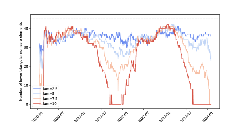
We use a half-life of $H=63$ (one quarter). We evaluate the model for $\lambda=2.5$, $5$, $7.5$, and $10$, which result in covariance estimates with inverses that are increasingly sparse.

Results.

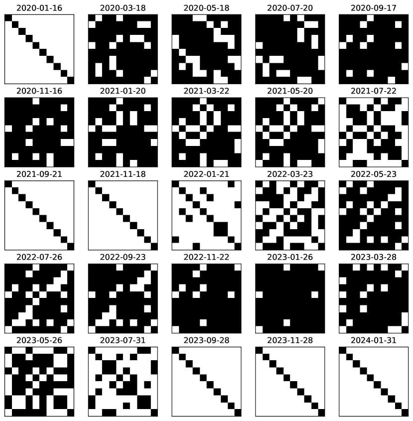
In figure 1 we show the sparsity of the inverse covariance matrix across time for the different values of $\lambda$. The plot gives the number of nonzero entries in the precision matrix, with the dashed line at 45 showing the maximum possible value, i.e., a fully dense precision matrix. We also show examples of the inverse covariance matrix sparsity patterns at evenly spaced times in figure 2. These plots show that the sparse inverse covariance estimate varies considerably with time, i.e., market conditions.

Figure 1: Number of nonzeros in the inverse covariance matrix across time for different values of $\lambda$.

Figure 2: Sparsity patterns at various times for $\lambda=10$. White boxes denote zero entries in the precision matrix.

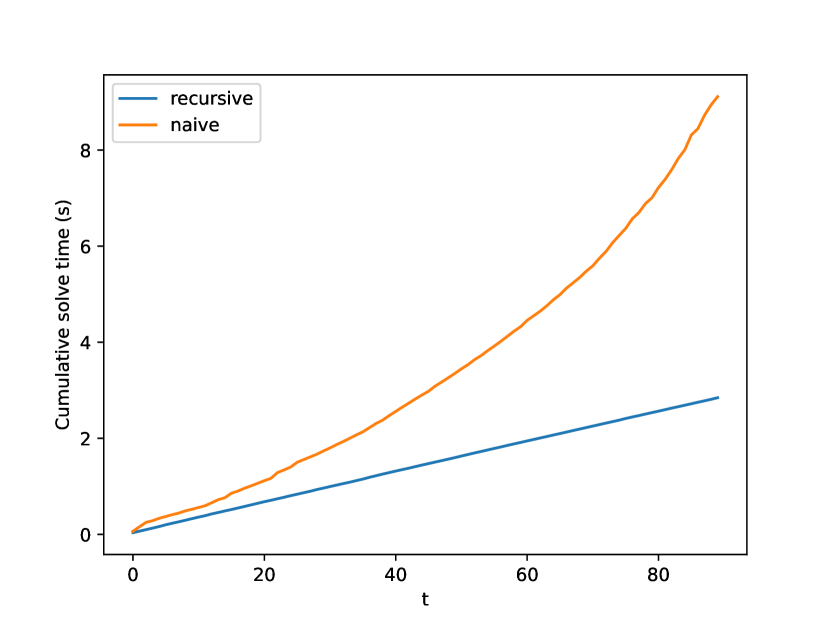
To illustrate the savings obtained from the recursive formulation, we show the running computation time of fitting the model in figure 3. As expected the naïve method, which saves all past data and directly computes the estimate using all past value, grows quadratically in time, whereas the recursive method grows linearly.

Figure 3: Cumulative time to fit the sparse inverse covariance estimation model using the naïve method and the (exact) recursive method.

5.2 Quantile estimation

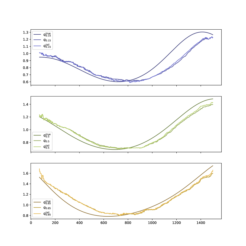
We use the pinball loss function (6) to estimate the 15th, 50th, and 85th percentiles of a scalar time series. Since the pinball loss is not twice differentiable, we use the tail approximation method described in §4.3 to fit the tail using points sampled from a normal distribution centered at the previous estimate with standard deviation equal to one fifth of the magnitude of the previous estimate.

Data.

In this example we use synthetic data. First we generate smoothly varying sequences $\mu_{t}$ and $\sigma_{t}$ as

$$\mu_{t} = a\sin(2\pi t/P_{1})+b\cos(2\pi t/P_{2}),\quad t=1,\ldots,T,$$

$$\sigma_{t} = c\sin(2\pi t/P_{3})+d\cos(2\pi t/P_{4}),\quad t=1,\ldots,T,$$

with periods

$$P_{1}=2100,\quad P_{2}=1500,\quad P_{3}=1100,\quad P_{4}=1700,$$

and coefficients

$$a=-.17,\quad b=.23,\quad c=-.12,\quad d=.13.$$

(There is no special significance to the specific form; this is just a simple way to generate a smoothly varying sequence.) Then we generate data as $x_{t}=\exp z_{t}$, with $z_{t}\sim\mathcal{N}(\mu_{t},\sigma_{t}^{2})$. The ‘true’ quantiles are then

$$\exp\left(\mu_{t}+\sigma_{t}\Phi^{-1}(\eta)\right),\qquad t=1,\ldots,T,\quad\eta=.15,.5,.85,$$

where $\Phi$ is the cumulative distribution function of a standard normal random variable.

Parameters.

The half-life is $H=100$, and the buffer sizes are $M=100$ and $M^{\text{tail}}=3M$. We sample $L=10$ points for the tail approximation.

Results.

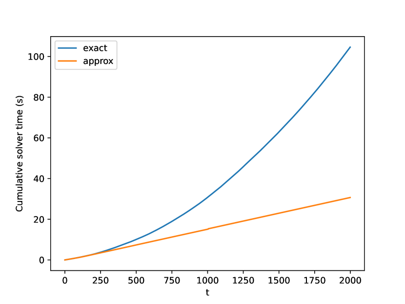
We see that the approximate finite memory EWMM is able to closely match the results of the exact method while incurring a fraction of the computational cost. We plot the true quantile value and the estimated quantile values across time in figure 4. We also show how the computational effort of the two methods compare in figure 5. We show four examples of the quadratic tail approximations in figure 6.

Figure 4: True and estimated quantile values across time using the exact and approximate finite memory EWMM methods.

Figure 5: Time to fit the quantile estimation model using the exact and approximate finite memory EWMM methods.

Figure 6: Quadratic tail approximations for the pinball loss.

5.3 Logistic regression

In this example, we generate data from a joint distribution of features and targets, and use the approximate finite memory EWMM for a logistic regression model to make predictions. We use the logistic loss function (7) and regularizer $r(\theta)=\lambda\|\theta\|_{2}^{2}$. We fit the approximate finite memory EWMM using the recursive Taylor approximation method described in §4.2.

Data.

We first generate a smoothly varying sequence of parameters $\theta_{t}^{\text{true}}\in{\mbox{\bf R}}^{3}$ as

$$\theta_{t}=a\sin(2\pi t/4000)+b\cos(2\pi t/6000),\quad t=1,\ldots,T=2000,$$

where

$$a=\begin{bmatrix}.17\\ .23\\ -.12\end{bmatrix},\quad b=\begin{bmatrix}.13\\ -.11\\ -.19\end{bmatrix}.$$

We then generate pairs $x_{t}=(z_{t},y_{t})$ for $t=1,\ldots,T$ as independent samples from the following joint distribution parametrized by $\theta_{t}^{\text{true}}$:

$$z_{t}\sim\mathcal{N}(\theta_{t}^{\text{true}},I),\qquad y_{t}=\mathop{\bf sign}(z_{t}^{T}\theta_{t}+\xi_{t}),\qquad\xi_{t}\sim\mathcal{N}(0,\sigma^{2}).$$

We use $\sigma=.1$.

Parameters.

We take $\lambda=0.5$, half-life $H=150$, and $M=H$.

Results.

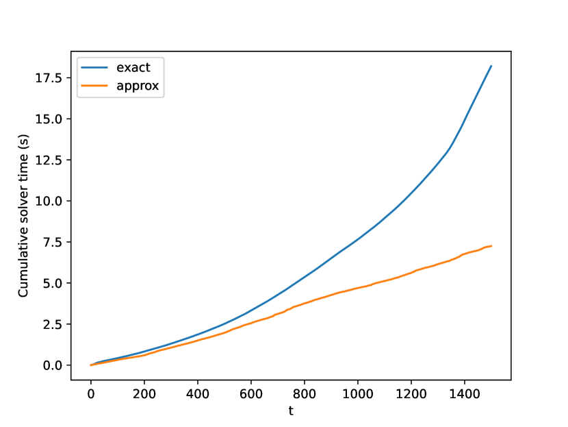
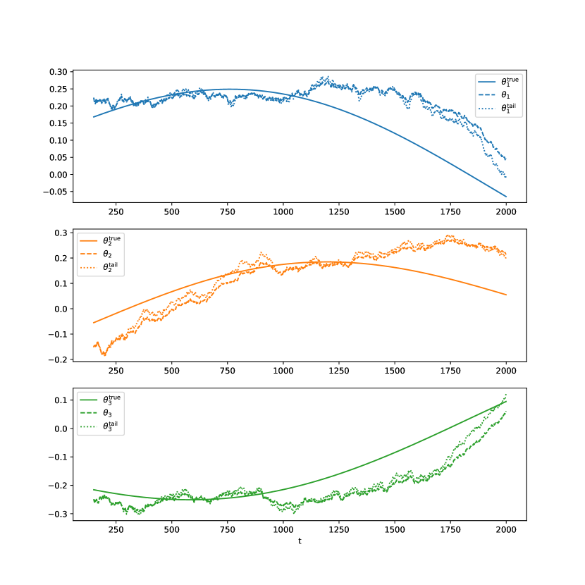
We show the true value $\theta_{t}^{\text{true}}$ and the estimate $\theta_{t}$ across time for the full and tail approximation models in figure 7. We see that the approximate finite memory EWMM is able to closely match the performance from the exact EWMM. We show the cumulative time to fit the model across time in figure 8.

Figure 7: True and estimated parameters for the logistic regression model.

Figure 8: Time to fit the logistic regression model using the exact and approximate finite memory EWMM methods.

6 Conclusions

We have introduced the general exponentially weighted moving model, which generalizes the well-known exponentially weighted moving average. The idea is simple, and closely related to other well-known methods.

When the loss is quadratic, a simple recursion can be used to exactly compute the EWMM estimate by forming and solving a fixed size problem. When the parameters are from an exponential family, we compute the EWMA of the sufficient statistic. This special case includes some obvious ones, such as least squares regression (possibly with nonquadratic regularizer), and some less obvious ones like sparse inverse covariance.

When the loss is not quadratic, a simple recursion cannot be used. Instead we propose an approximate method that stores a fixed window of data and carries out computation that does not grow with time.

In this paper we do not suggest or recommend EWMMs for applications; we simply address the question of how to compute it, or an approximation of it, efficiently.

References

- [Dar35] Georges Darmois “Sur les lois de probabilites estimation exhaustive” In C.R. Acad. Sci. Paris 200, 1935, pp. 1265–1266
- [Koo36] Bernard Koopman “On distributions admitting a sufficient statistic” In Transactions of the American Mathematical Society 39.3, 1936, pp. 399–409
- [Pit36] Edwin Pitman “Sufficient statistics and intrinsic accuracy” In Mathematical Proceedings of the Cambridge Philosophical Society 32.4, 1936, pp. 567–579 Cambridge University Press
- [Bro56] R. Brown “Exponential smoothing for predicting demand” In Philip Morris Records; Master Settlement Agreement, 1956, pp. 15 URL: https://www.industrydocuments.ucsf.edu/docs/jzlc0130
- [Sob67] Ilya Sobol “On the distribution of points in a cube and the approximate evaluation of integrals” In Zhurnal Vychislitel’noi Matematiki i Matematicheskoi Fiziki 7.4 Russian Academy of Sciences, Branch of Mathematical Sciences, 1967, pp. 784–802
- [Sor70] H. Sorenson “Least-squares estimation: from Gauss to Kalman” In IEEE Spectrum 7.7, 1970, pp. 63–68 DOI: 10.1109/MSPEC.1970.5213471
- [Chr71] W. Christiaanse “Short-Term Load Forecasting Using General Exponential Smoothing” In IEEE Transactions on Power Apparatus and Systems PAS-90.2, 1971, pp. 900–911 DOI: 10.1109/TPAS.1971.293123
- [KBJ78] R. Koenker and G. Bassett Jr “Regression quantiles” In Econometrica: Journal of the Econometric Society JSTOR, 1978, pp. 33–50
- [Cle79] W. Cleveland “Robust locally weighted regression and smoothing scatterplots” In Journal of the American statistical association 74.368 Taylor & Francis, 1979, pp. 829–836
- [JC85] Raj Jain and Imrich Chlamtac “The P2 algorithm for dynamic calculation of quantiles and histograms without storing observations” In Communications of the ACM 28.10 ACM New York, NY, USA, 1985, pp. 1076–1085
- [TH87] Robert Tibshirani and Trevor Hastie “Local likelihood estimation” In Journal of the American Statistical Association 82.398 Taylor & Francis, 1987, pp. 559–567
- [GVL89] G. Golub and C. Van Loan “Matrix computations” JHU press, 1989
- [Hub92] Peter Huber “Robust Estimation of a Location Parameter” In Breakthroughs in Statistics: Methodology and Distribution New York, NY: Springer New York, 1992, pp. 492–518 DOI: 10.1007/978-1-4612-4380-9˙35
- [BT95] P. Boggs and J. Tolle “Sequential quadratic programming” In Acta Numerica 4 Cambridge University Press, 1995, pp. 1–51
- [GS95] Carl Gauss and G. Stewart “Theory of the Combination of Observations Least Subject to Errors” SIAM, 1995
- [Tib96] Robert Tibshirani “Regression Shrinkage and Selection via the Lasso” In Journal of the Royal Statistical Society. Series B (Methodological) 58.1 [Royal Statistical Society, Wiley], 1996, pp. 267–288
- [OSB99] A.V. Oppenheim, R.W. Schafer and J.R. Buck “Discrete-time Signal Processing” Prentice Hall, 1999
- [GK01] Michael Greenwald and Sanjeev Khanna “Space-efficient online computation of quantile summaries” In SIGMOD Rec. 30.2 New York, NY, USA: Association for Computing Machinery, 2001, pp. 58–66
- [HTF01] Trevor Hastie, Robert Tibshirani and Jerome Friedman “The Elements of Statistical Learning: Data Mining, Inference, and Prediction” Springer, 2001
- [Tsa02] Ruey Tsay “Analysis of Financial Time Series” John Wiley & Sons, 2002
- [BV04] S. Boyd and L. Vandenberghe “Convex Optimization” Cambridge University Press, 2004
- [VDMW04] Rudolph Van Der Merwe and Eric Wan “Sigma-point kalman filters for probabilistic inference in dynamic state-space models” Oregon Health & Science University, 2004
- [FHT07] Jerome Friedman, Trevor Hastie and Robert Tibshirani “Sparse inverse covariance estimation with the Lasso”, 2007 arXiv:0708.3517 [stat.ME]
- [WB09] Yang Wang and Stephen Boyd “Performance bounds for linear stochastic control” In Systems & Control Letters 58.3 Elsevier, 2009, pp. 178–182
- [MOW11] J. Menchero, D. Orr and J. Wang “The Barra US equity model (USE4), methodology notes” MSCI Barra, 2011
- [Pow11] Warren Powell “Approximate Dynamic Programming: Solving the Curses of Dimensionality” John Wiley & Sons, 2011
- [KB14] Arezou Keshavarz and Stephen Boyd “Quadratic approximate dynamic programming for input-affine systems” In International Journal of Robust and Nonlinear Control 24.3 Wiley Online Library, 2014, pp. 432–449
- [Box+15] George Box, Gwilym Jenkins, Gregory Reinsel and Greta Ljung “Time Series Analysis: Forecasting and Control” John Wiley & Sons, 2015
- [WOB15] Yang Wang, Brendan O’Donoghue and Stephen Boyd “Approximate dynamic programming via iterated Bellman inequalities” In International Journal of Robust and Nonlinear Control 25.10 Wiley Online Library, 2015, pp. 1472–1496
- [DB16] S. Diamond and S. Boyd “CVXPY: A Python-embedded modeling language for convex optimization” In Journal of Machine Learning Research 17.83, 2016, pp. 1–5
- [Haz16] Elad Hazan “Introduction to online convex optimization” In Foundations and Trends in Optimization 2.3-4 Now Publishers, Inc., 2016, pp. 157–325
- [McM17] H. McMahan “A survey of algorithms and analysis for adaptive online learning” In The Journal of Machine Learning Research 18.1 JMLR.org, 2017, pp. 3117–3166
- [KW19] Mykel Kochenderfer and Tim Wheeler “Algorithms for Optimization” Mit Press, 2019
- [TB21] Jonathan Tuck and Stephen Boyd “Fitting Laplacian regularized stratified Gaussian models” In Optimization and Engineering Springer, 2021, pp. 1–21
- [Ber22] Dimitri Bertsekas “Abstract Dynamic Programming” Athena Scientific, 2022
- [KWW22] Mykel Kochenderfer, Tim Wheeler and Kyle Wray “Algorithms for Decision Making” MIT press, 2022
- [Joh+23] Kasper Johansson et al. “A Simple Method for Predicting Covariance Matrices of Financial Returns” In Foundations and Trends in Econometrics 12.4, 2023, pp. 324–407
- [Fre24] Kenneth French “French Data Library”, http://mba.tuck.dartmouth.edu/pages/faculty/ken.french/data_library.html, 2024