Spurious Stationarity and Hardness Results for Mirror Descent

Abstract

Despite the considerable success of Bregman proximal-type algorithms, such as mirror descent, in machine learning, a critical question remains: Can existing stationarity measures, often based on Bregman divergence, reliably distinguish between stationary and non-stationary points? In this paper, we present a groundbreaking finding: All existing stationarity measures necessarily imply the existence of spurious stationary points. We further establish an algorithmic independent hardness result: Bregman proximal-type algorithms are unable to escape from a spurious stationary point in finite steps when the initial point is unfavorable, even for convex problems. Our hardness result points out the inherent distinction between Euclidean and Bregman geometries, and introduces both fundamental theoretical and numerical challenges to both machine learning and optimization communities.

Keywords: Nonconvex Optimization, Bregman Geometry, Spurious Stationary Point

1 Introduction

This paper focuses on structured nonsmooth nonconvex optimization problems of the form

$$\min\limits_{\bm{x}\in{\mathbb{R}}^{n}}F(\bm{x})\coloneqq f(\bm{x})+g(\bm{x}),$$ (P)

where $\operatorname{dom}(g)={\cal X}$ is a nonempty closed convex set, $f:{\mathbb{R}}^{n}\rightarrow{\mathbb{R}}$ is continuously differentiable on ${\cal X}$, and $g:{\mathbb{R}}^{n}\rightarrow\overline{\mathbb{R}}$ is a convex and locally Lipschitz continuous function.

To address (P), Bregman proximal gradient descent and its variants are among the most popular first-order optimization methods for both convex and nonconvex scenarios (Bauschke et al.,, 2017; Solomon et al.,, 2016; Zhang et al.,, 2021; Zhu et al.,, 2021). At each iteration $k$, we update the iterate according to

$$\bm{x}^{k+1}=\mathop{\operatorname{argmin}}\limits_{\bm{y}\in{\mathbb{R}}^{n}}\ \left\{\gamma\left(\bm{y};\bm{x}^{k}\right)+g(\bm{y})+\frac{1}{t_{k}}D_{h}(\bm{y},\bm{x}^{k})\right\},$$ (1.1)

where $t_{k}\geq 0$ is the step size at the $k$-th iteration, $D_{h}$ is the Bregman divergence associated with a kernel function $h$, and $\gamma(\ \cdot\ ;\bm{x}^{k})$ is the surrogate model at the point $\bm{x}^{k}$. Certainly, we have the option to pick the surrogate function $\gamma$ as the original function $f$. In this context, the update rule (1.1) can encompass the Bregman proximal point method (Chen and Teboulle,, 1993; Kiwiel,, 1997). When the surrogate model takes the form of a linear model, specifically $\gamma(\bm{y};\bm{x}^{k}):=f(\bm{x}^{k})+\nabla f(\bm{x}^{k})^{T}(\bm{x}-\bm{x}^{k})$, the update (1.1) covers the Bregman proximal gradient descent method (BPG) (Bauschke et al.,, 2017, 2019; Censor and Zenios,, 1992; Xu et al., 2019b, ; Zhu et al.,, 2021). This method includes the standard proximal gradient descent method as a special case when we choose $h(\bm{x})=\tfrac{1}{2}\|\bm{x}\|^{2}$. Alternatively, one can opt for a quadratic surrogate model, i.e., $\gamma(\bm{y};\bm{x}^{k}):=f(\bm{x}^{k})+\nabla f(\bm{x}^{k})^{T}(\bm{x}-\bm{x}^{k})+\frac{1}{2}(\bm{x}-\bm{x}^{k})^{T}\nabla^{2}f(\bm{x}^{k})(\bm{x}-\bm{x}^{k})$, which has been recently explored by Doikov and Nesterov, (2023).

To understand how the sequence of iterations behaves and how close it gets to convergence, researchers typically propose a residual function ${R}:{\mathbb{R}}^{n}\rightarrow{\mathbb{R}}_{+}$ that measures the stationarity of the iterations. Then, a common way to conduct the convergence analysis in the literature is to establish the convergence of the sequence $\{{R}(\bm{x}^{k})\}_{k\in{\mathbb{N}}}$. Nevertheless, within the general setup, a definitive answer to the following question remains unknown:

$$\boxed{\vspace{2mm}\lim_{k\to\infty}{R}(\bm{x}^{k})=0\,\,\,\mathop{\Longleftrightarrow}_{?}\,\,\,{\bf{0}}\in\partial F\left(\lim_{k\to\infty}\bm{x}^{k}\right).\vspace{2mm}}$$ (Q)

To establish this equivalence (Q), we have to check: (1) The residual function ${R}$ is continuous; (2) $R(\bm{x})$ equals zero if and only if $\bm{x}$ is a stationary point. Otherwise, the sequence of iterates may not converge to the desired point.

In the literature, there are two commonly used stationarity measures. The first one, as proposed by Zhang and He, (2018), quantifies stationarity by evaluating the gap between the current iterate and its Bregman proximal point. Another popular choice is to use the distance between two consecutive iterates, see Bedi et al., (2022); Huang et al., 2022a ; Huang et al., 2022b ; Latafat et al., (2022). The validity of the equivalence (Q) for them is only established when the gradient of the kernel function is Lipschitz. Then, we can observe the non-degenerate property of the mirror map, where Euclidean and Bregman geometries align. Therefore, demonstrating the continuity of ${R}$, as well as establishing the necessity and sufficiency of ${R}$, are straightforward. Nonetheless, in the case of a kernel whose gradient is not Lipschitz continuous, such as the entropy kernel, the equivalence (Q) is much less investigated. Moreover, the stationarity measure proposed by Zhang and He, (2018) is not even well-defined on the boundary of $\operatorname{dom}(h)$ for non-Lipschitz kernels, let alone being continuous across the entire domain.

In this paper, we first introduce an extended Bregman stationarity measure that unifies and extends the previously two mentioned stationarity measures, which is well-defined over the closure of the entire domain $\operatorname{cl}(\operatorname{dom}(h))$. The key insight lies in defining stationarity on the boundary and subsequently demonstrating the continuity of this novel stationarity measure on the entire domain. Then, we proceed to check its applicability across a broader spectrum of separable (potentially non-gradient Lipschitz) kernel functions.

To start, we provide an affirmative answer regarding necessity: Our extended Bregman stationarity measure equals zero when the point is stationary. However, the sufficiency fails due to the presence of spurious stationary points that we have identified. That is, there are points (named spurious stationary points) at which the extended Bregman stationarity measure equals zero, but they do not qualify as stationary points. We show that in fact spurious stationary points generally exist even in a simple group of convex problems, for all existing Bregman stationarity measures.

Building upon the discovery of spurious stationary points mentioned earlier, we can further establish a hardness result: Regardless of the number of steps taken, the sequence generated by the Bregman proximal-type update (1.1) can remain within a small neighborhood of these spurious points. Our discovery of spurious stationary points sheds light on the underlying challenges in the design and analysis of Bregman divergence-based methods—a facet that has been overlooked by the research community for an extended period. Our paper serves as an initial step in acknowledging this issue and offering fundamental insights and findings.

Notation.

The set of all integers up to $n\in\mathbb{N}$ is denoted by $[n]=\{1,\ldots,n\}$, and the sets of real numbers, non-negative real numbers, non-positive numbers and extended real numbers are denoted by ${\mathbb{R}}$, ${\mathbb{R}}_{+}$, ${\mathbb{R}}_{-}$, and $\overline{{\mathbb{R}}}$, respectively. Bold letters such as $\bm{x}$, $\bm{y}$ stand for vectors, and calligraphic letters such as ${\cal X}$, $\mathcal{Y}$ denote sets. The $i$-th coordinate of $\bm{x}$ is represented by $x_{i}$, and $\bm{x}_{\mathcal{I}}$ denotes a subvector obtained by selecting a subset of indices $\mathcal{I}$ from the vector $\bm{x}$. We use $\bm{x}^{k}\to\bm{x}$ as a shorthand for $\lim_{k\to\infty}\bm{x}^{k}=\bm{x}$. Given a set $\mathcal{X}$, we use $\operatorname{cl}({\cal X})$, ${\rm int}({\cal X})$, and $\operatorname{bd}({\cal X})$ to denote its closure, interior, and boundary, respectively. The Euclidean ball ${\mathbb{B}}_{\epsilon}(\bm{x})$ is defined through ${\mathbb{B}}_{\epsilon}(\bm{x}):=\{\bm{y}\in{\mathbb{R}}^{n}:\|\bm{x}-\bm{y}\|_{2}\leq\epsilon\}$. We define the domain of the function $\phi:{\mathbb{R}}^{n}\rightarrow\overline{\mathbb{R}}$, denoted by $\text{dom}(\phi)$, as the set $\{\bm{x}\in{\mathbb{R}}^{n}:\phi(\bm{x})<+\infty\}$. Finally, the indicator function $\delta_{{\cal X}}$ of a set ${\cal X}\subseteq{\mathbb{R}}^{n}$ is defined through $\delta_{{\cal X}}(\bm{x})=0$ if $\bm{x}\in{\cal X}$; $\delta_{{\cal X}}(\bm{x})=+\infty$ otherwise. We employ the shorthand $\delta_{{\mathbf{g}}(\bm{x})={\mathbf{0}}}$ to compactly represent $\delta_{\{\bm{x}\in{\mathbb{R}}^{n}:{\mathbf{g}}(\bm{x})={\mathbf{0}}\}}$ for any real-valued function $g:{\mathbb{R}}^{n}\rightarrow{\mathbb{R}}$.

Organization.

The remainder of this paper is organized as follows. In Sec. 2, we present and justify the assumptions we make throughout this paper. In Sec. 3, we introduce the extended Bregman stationarity measure and establish its continuity on the entire domain. Then, we verify the necessity of zero extended stationarity measure at any stationary point. In Sec. 4, we unveil the existence of spurious stationary points and show the insufficiency of zero extended stationarity measure for stationarity. In Sec. 5, we provide a general hardness result for Bregman proximal-type methods and offer several interesting hard instances.

2 Assumptions and justification

In this section, we state our blanket assumptions and justify their validity in applications.

Assumption 1 (Problem (P)).

Let $\operatorname{dom}(g)={\cal X}$ be a nonempty closed convex set. The following hold.

1. The function $f$ is continuously differentiable on ${\cal X}$.

2. The function $g$ is convex and locally Lipschitz continuous on ${\cal X}$.

3. There exists a strictly feasible point $\bm{x}^{{\rm{int}}}\in{\rm{int}}(\operatorname{dom}(h))\cap{\cal X}$ and ${\cal X}\subseteq\operatorname{cl}(\operatorname{dom}(h))$.

4. The function $h$ is a separable kernel function, see Definition 1.

Assumptions 1 (i)-(iii) or their stronger versions are widely adopted in the literature; see, e.g., Assumption A in Bauschke et al., (2017), Assumption A in Bauschke et al., (2019), and Definition 1 and Assumption 1 in Azizian et al., (2022). We also refer the readers to see the practical problems that satisfy these assumptions and are solved by Bregman proximal-type methods satisfying these assumptions in, e.g., problem (3) in Xu et al., 2019a , and problem (6) in Xu et al., 2019b and problem (7) in Chen et al., (2020).

We proceed to justify the applicability of Assumption 1 (iv). To do so, we introduce the definition of a separable kernel function, which plays a crucial role in delineating the geometry induced by Bregman divergence.

Definition 1 (Separable kernel function).

We define the separable kernel function $h:{\mathbb{R}}^{n}\rightarrow\overline{\mathbb{R}}$ as

1. The kernel function $h$ is defined through $h(\bm{x})=\sum_{i=1}^{n}\varphi(x_{i})$, where $\varphi:{\mathbb{R}}\rightarrow\overline{\mathbb{R}}$ is a univariate function.

2. $\varphi$ is continuously differentiable on ${\rm{int}}(\operatorname{dom}(\varphi))$, and $|\varphi^{\prime}(x^{k})|\to+\infty$ as $x^{k}\to x\in{\rm{bd}}(\operatorname{dom}(\varphi))$;

3. $\varphi$ is strictly convex.

The separability structure outlined in property (i) is ubiquitous in real-world scenarios (Bauschke et al.,, 2019; Azizian et al.,, 2022; Li et al.,, 2023). We illustrate its practicality by presenting several widely used separable kernel functions, which meet Definition 1.

Example 1.

1. Boltzmann–Shannon entropy kernel $h(\bm{x})=\sum_{i=1}^{n}x_{i}\log(x_{i})$;

2. Fermi–Dirac entropy kernel $h(\bm{x})=\sum_{i=1}^{n}x_{i}\log(x_{i})+(1-x_{i})\log(1-x_{i})$;

3. Burg entropy kernel $h(\bm{x})=\sum_{i=1}^{n}-\log(x_{i})$;

4. Fractional power kernel $h(\bm{x})=\sum_{i=1}^{n}px_{i}-\frac{x_{i}^{p}}{1-p}$ ($0<p<1$);

5. Hellinger entropy kernel $h(\bm{x})=\sum_{i=1}^{n}-\sqrt{1-x_{i}^{2}}$.

Remark 1.

The implication of the separable structure is that $\operatorname{cl}(\operatorname{dom}(h))$ forms a box, i.e.,

$$\operatorname{cl}(\operatorname{dom}(h))=[a,c]\times[a,c]\times\cdots\times[a,c],$$

where $a,c\in{{\mathbb{R}}}\cup\{\pm\infty\}$ with $\operatorname{cl}(\operatorname{dom}(\varphi))=[a,c]$. Due to the convexity of $\varphi$ and Definition 1 (ii), $\varphi^{\prime}$ is monotonically increasing and further $\varphi^{\prime}(x)\to-\infty$ (resp. $+\infty$) if $x\to a^{+}$ (resp. $x\to c^{-}$) and $a>-\infty$ (resp. $c<+\infty$).

Properties (ii) and (iii) are referred to as Legendre-type properties, as defined in Bauschke et al., (2017), and they are common in the kernel functions used in the literature.

Next, we proceed to give assumptions of algorithm classes (i.e., the update rule (1.1)), which is characterized by the surrogate model $\gamma$.

Assumption 2 (Surrogate model $\gamma$).

The following hold.

1. The function $\gamma(\bm{y};\bm{x})$ and gradient $\nabla\gamma(\bm{y};\bm{x})$ (w.r.t $\bm{y}$) are jointly continuous w.r.t. $(\bm{y},\bm{x})$ , i.e.,

   $$\lim\limits_{(\bm{y}^{\prime},\bm{x}^{\prime})\to(\bm{y},\bm{x})}\gamma(\bm{y}^{\prime};\bm{x}^{\prime})=\gamma(\bm{y};\bm{x})\text{ and }\lim\limits_{(\bm{y}^{\prime},\bm{x}^{\prime})\to(\bm{y},\bm{x})}\nabla\gamma(\bm{y}^{\prime};\bm{x}^{\prime})=\nabla\gamma(\bm{y};\bm{x}),$$

   for all $\bm{y}\in{\cal X}$ and $\bm{x}\in{\cal X}$.

2. For all $\bm{x}\in{\cal X}$, we have

   $$\nabla\gamma(\bm{y};\bm{x})\mid_{\bm{y}=\bm{x}}=\nabla f(\bm{x}),\text{ and }\gamma(\bm{y};\bm{x})\mid_{\bm{y}=\bm{x}}=f(\bm{x}).$$

3. For all $\bm{x}\in{\cal X}$, there exists a constant $\overline{t}>0$ such that $\overline{t}\gamma(\ \cdot\ ;\bm{x})+h(\cdot)$ is strictly convex.

4. Either ${\cal X}$ is compact or we have the following condition: For all step sizes $t\in(0,\overline{t}]$ and all sequences $\{\bm{x}^{k}\}_{k\in{\mathbb{N}}},\{\bm{y}^{k}\}_{k\in{\mathbb{N}}}\subseteq{\rm int}(\operatorname{dom}(h))\cap{\cal X}$ such that $\|\bm{y}^{k}\|\to\infty$ and $\bm{x}^{k}\to\overline{\bm{x}}\in{\cal X}$, the following holds:

   $$\lim\limits_{k\to\infty}\gamma(\bm{y}^{k};\bm{x}^{k})+g(\bm{y}^{k})+\frac{1}{t}D_{h}(\bm{y}^{k},\bm{x}^{k})=+\infty,$$ (2.1)

   where $D_{h}(\bm{y},\bm{x})\coloneqq h(\bm{y})-h(\bm{x})-h^{\prime}(\bm{x})(\bm{y}-\bm{x})$.

Unless otherwise specified, the step size $t$ in this paper is assumed to satisfy $t\in(0,\overline{t}]$.

Assumptions 2 (i) and (ii) are standard, serving to ensure the continuity and local correctness of the surrogate model $\gamma$. Assumption 2 (iii) usually reduces to conditions commonly adopted in the literature or is automatically satisfied for all three choices mentioned in the introduction. When $\gamma$ represents the first-order expansion of $f$ at the current iterate $\bm{x}$, Assumption 2 (iii) is trivially satisfied. If $\gamma$ is selected as the original function $f$, it reduces to the relatively weak convexity condition, as discussed in Bolte et al., (2018); Zhang and He, (2018). When $\gamma$ is the second-order expansion of $f$ at the current iterate $\bm{x}$, the $L$-smoothness of $f$ and strong convexity of $h$ suffice to guarantee Assumption 2 (iii).

The most subtle condition is Assumption 2 (iv), which is to ensure the well-posedness of the Bregman proximal-type update (1.1). If ${\cal X}$ is unbounded, then Assumption 2 (iv) can be implied by supercoercive-type conditions, see Lemma 2 in Bauschke et al., (2017) and Assumption B in Bolte et al., (2018). Without Assumption 2 (iv), the update (1.1) may not have an optimal solution. Interested readers are referred to Appendix B for the rigorous verification of this assumption for commonly used $\gamma$. Here, we provide a simple example demonstrating its necessity.

Example 2 (Necessity of Assumption 2 (iv)).

Let $h(x)=1/x$, $g(x)=\delta_{{\mathbb{R}}_{+}}(x)$, $f(x)=(x-3)^{2}$, and $\gamma(y;x)=(x-3)^{2}+2(x-3)(y-x)$. Assumption 1 and Assumptions 2 (i)–(iii) hold for this problem with any $\bar{t}>0$. We can verify that Assumption 2 (iv) fails when we pick $x^{k}=\frac{1}{2}+\frac{1}{2^{k}}$, $y^{k}=2^{k}$ and $t=1$. It turns out that the well-posedness of (1.1) does not hold. For all $x\in[\frac{1}{2},1]$ and $t=1$, we have

$$\mathop{\operatorname{argmin}}\limits_{y\in{\mathbb{R}}_{+}}\ \left\{\gamma\left(y;x\right)+\frac{1}{t}D_{h}(y,x)\right\}$$

$$= \mathop{\operatorname{argmin}}\limits_{y\in{\mathbb{R}}_{+}}\ \left\{\frac{1}{y}+\left(2x+\frac{1}{x^{2}}-6\right)(y-x)\right\}=\varnothing,$$

where the last equality is due to $2x+\tfrac{1}{x^{2}}-6\leq-1$ for $x\in[\frac{1}{2},1]$.

Based on Assumptions 1 and 2, we present the following lemma, which discusses the well-posedness of update (1.1) on ${\rm int}(\operatorname{dom}(h))$. Similar results can also be found in Bauschke et al., (2017); Dragomir et al., (2022).

Lemma 1.

For all $\bm{x}\in{\rm int}(\operatorname{dom}(h))\cap{\cal X}$, we have ${T}^{t}_{\gamma}(\bm{x})\in{\rm{int}}(\operatorname{dom}(h))\cap{\cal X}$.

Here, the update mapping ${T}^{t}_{\gamma}$ is defined through ${T}^{t}_{\gamma}\coloneqq\operatorname{argmin}_{\bm{y}}\ \gamma(\bm{y};\bm{x}^{k})+g(\bm{y})+\frac{1}{t}D_{h}(\bm{y},\bm{x}^{k})$, see the update (1.1). Lemma 1 claims that the sequence generated by Bregman proximal-type methods, as outlined in Algorithm 1, remains within the interior ${\rm int}(\operatorname{dom}(h))$.

Algorithm 1 Bregman divergence-based algorithms

0:   $\{t_{k}\}_{k\in{\mathbb{N}}}$ with $t_{k}>0$, initial point $\bm{x}^{0}\in{\rm int}(\operatorname{dom}(h))\cap{\cal X}$ and $k=0$.

  while  Stopping Criteria is not satisfied  do

     $\bm{x}^{k+1}=T^{t_{k}}_{\gamma}(\bm{x}^{k})$.

     Set $k=k+1$.

  end while

  $\bm{x}^{k}$

3 Extended Bregman stationarity measure

In this section, our goal is to introduce the extended Bregman stationarity measure and investigate its continuity and necessity later. To start, we will give the definition of Bregman proximal mapping, which serves as a crucial tool in connecting our stationarity measure with existing ones.

Definition 2 (Bregman proximal mapping).

(Bauschke et al.,, 2018; Lau and Liu,, 2022) For $t>0$ and a kernel function $h:{\mathbb{R}}^{n}\rightarrow\overline{\mathbb{R}}$, the Bregman proximal mapping for $F:{\rm int}(\operatorname{dom}(h))\to\overline{\mathbb{R}}$ is defined by

$${{\rm{prox}}}^{t}_{h,F}(\bm{x})=\underset{\bm{y}\in{\mathbb{R}}^{n}}{\operatorname{argmin}}\left\{F(\bm{y})+\frac{1}{t}D_{h}(\bm{y},\bm{x})\right\}.$$

All existing stationarity measures can be unified as

$$R^{t}_{\gamma}(\bm{x})\coloneqq D_{h}(T^{t}_{\gamma}(\bm{x}),\bm{x}),$$

where $t>0$ is the step size. Conceptually, we use the relative change under the Bregman geometry to quantify the stationarity, which has been well explored in the literature (Bedi et al.,, 2022; Huang et al., 2022a, ; Huang et al., 2022b, ; Latafat et al.,, 2022). If we set $\gamma=f$, then the update mapping $T^{t}_{\gamma}(\bm{x})$ coincides with ${\rm{prox}}^{t}_{h,F}(\bm{x})$, and thus $R^{t}_{\gamma}$ recovers the stationarity gap $D_{h}({\rm{prox}}_{h,F}^{t}(\bm{x}),\bm{x})$ proposed by Zhang and He, (2018). As we can see, $R^{t}_{\gamma}$ unifies the two popular stationarity measures used in the literature. Unfortunately, $R^{t}_{\gamma}$ is not well-defined on the boundary $\operatorname{bd}(\operatorname{dom}(h))$, as the mapping $\bm{x}\mapsto T^{t}_{\gamma}(\bm{x})$ defined by (1.1) involves the Bregman divergence function $(\bm{y},\bm{x})\mapsto D_{h}(\bm{y},\bm{x})$, which is only defined on $\operatorname{dom}(h)\times{\rm int}(\operatorname{dom}(h))$. Given this limitation, we are motivated to extend the domain of Bregman stationarity measures to $\operatorname{cl}(\operatorname{dom}(h))$. As a preliminary action, we define the extended update mapping, applicable to $\operatorname{cl}(\operatorname{dom}(h))\cap{\cal X}$.

Definition 3 (Extended update mapping).

We define the extended mapping $\overline{T}^{t}_{\gamma}(\bm{x})$ as $\mathop{\operatorname{argmin}}\limits_{\bm{y}\in{\cal X}}\ G^{t}_{\gamma}(\bm{y};\bm{x})$, where $G^{t}_{\gamma}$ is defined by

$$G^{t}_{\gamma}(\bm{y};\bm{x})\coloneqq\gamma(\bm{y};\bm{x})+g(\bm{y})+\underbrace{\frac{1}{t}\sum_{i\in{\cal I}(\bm{x})}D_{\varphi}(y_{i},x_{i})}_{\textrm{Interior coordinates}}+\underbrace{\delta_{\bm{y}_{{\cal B}(\bm{x})}=\bm{x}_{{\cal B}(\bm{x})}}(\bm{y})}_{\textrm{Boundary coordinates}},$$

where ${\cal B}(\bm{x})\coloneqq\left\{b\in[n]:x_{b}\in{\rm{bd}}\left(\operatorname{dom}(\varphi)\right)\right\}$ and ${\cal I}(\bm{x})\coloneqq\left\{i\in[n]:x_{i}\in{\rm{int}}\left(\operatorname{dom}(\varphi)\right)\right\}$.

This newly updated rule distinguishes between interior and boundary coordinates. For boundary coordinates of $\bm{x}$, we enforce $\bm{y}$ to be equal to $\bm{x}$, while for interior coordinates, we update following the original update rule (1.1). This construction enables us to focus on the boundary points to address non-gradient Lipschitz kernel functions.

Remark 2.

(i) Due to Assumptions 2 (i) and (iv), the level sets of $G^{t}_{\gamma}(\ \cdot\ ;\bm{x})$ are compact, ensuring that $\mathop{\operatorname{argmin}}{\bm{y}}\ G^{t}_{\gamma}(\bm{y};\bm{x})\neq\varnothing$. Further details can be found in Fact 2 in the appendix. Additionally, Assumption 2 (iii) guarantees the strict convexity of $G^{t}_{\gamma}(\ \cdot\ ;\bm{x})$. Both the strict convexity and level boundedness of $G^{t}_{\gamma}$ ensure the well-definedness and uniqueness of the extended update mapping $\overline{T}^{t}_{\gamma}$. (ii) For all $\bm{x}\in{\rm int}(\operatorname{dom}(h))$, we have ${\cal I}(\bm{x})=[n]$ and then we can conclude that $\overline{T}^{t}_{\gamma}(\bm{x})=T^{t}_{\gamma}(\bm{x})$ by definition. (iii) As a byproduct, if we choose $\gamma(\bm{y};\bm{x})$ to be $f(\bm{y})$, then we obtain an extension of Bregman proximity operator $\overline{{\rm{prox}}}^{t}_{h,F}:\operatorname{cl}(\operatorname{dom}(h))\to{\mathbb{R}}^{n}$.

Armed with the extended update mapping $\overline{T}^{t}_{\gamma}$, we are now ready to provide the formal definition of the extended Bregman stationarity measure.

Definition 4 (Extended stationarity measure).

We define the extended Bregman stationarity measure $\overline{R}^{t}_{\gamma}(\bm{x}):{\cal X}\to{\mathbb{R}}$ as

$$\overline{R}^{t}_{\gamma}(\bm{x})\coloneqq\sum_{i\in{\cal I}(\bm{x})}D_{\varphi}\left(\overline{T}^{t}_{\gamma}(\bm{x})_{i},x_{i}\right).$$

It is worth noting that $\overline{R}^{t}_{\gamma}$ is defined over the entire domain ${\cal X}$, and it retrieves ${R}^{t}_{\gamma}(\mathbf{x})$ for $\bm{x}\in{\rm{int}}(\text{dom}(h))\cap{\cal X}$.

3.1 Continuity of extended stationarity measure

To investigate the equivalence described in (Q), our first step is to establish the continuity of $\overline{R}^{t}_{\gamma}$. This task involves recognizing that $\overline{R}^{t}_{\gamma}$’s definition depends on both $\overline{T}^{t}_{\gamma}$ and ${\cal I}(\bm{x})$, which may exhibit discontinuity.

To start, we establish the continuity of the extended update mapping:

Proposition 1 (Continuity of $\overline{T}^{t}_{\gamma}$).

The extended update mapping $\overline{T}^{t}_{\gamma}:\mathcal{X}\rightarrow\mathbb{R}^{n}$ is continuous on the domain $\mathcal{X}$.

Remark 3.

With the continuity of $\overline{T}^{t}_{\gamma}$, we can examine the definition of $\overline{T}^{t}_{\gamma}$ at $\bm{x}\in\operatorname{bd}(\operatorname{dom}(h))\cap{\cal X}$. It becomes apparent that $\overline{T}^{t}_{\gamma}(\bm{x})$ can be regarded as the limit of $\{\overline{T}^{t}_{\gamma}(\bm{x}^{k})\}_{k\in{\mathbb{N}}}$ for all sequences $\{\bm{x}^{k}\}_{k\in{\mathbb{N}}}\subseteq{\rm int}(\operatorname{dom}(h))\cap{\cal X}$ converging to $\bm{x}$.

The continuity of $\overline{T}^{t}_{\gamma}$ on ${\cal X}$ serves as a fundamental property of the extended update mapping. Not only does it provide insight into $\overline{T}^{t}_{\gamma}(\bm{x})$ for $\bm{x}\in\operatorname{bd}(\operatorname{dom}(h))\cap{\cal X}$, but it also plays a crucial role in establishing the continuity of $\overline{R}^{t}_{\gamma}$. Leveraging the continuity of $\overline{T}^{t}_{\gamma}$ and the structure of ${\cal I}(\bm{x})$, we establish one of the main theoretical results as below:

Theorem 1 (Continuity of $\overline{R}^{t}_{\gamma}$).

The extended stationarity measure $\overline{R}^{t}_{\gamma}:\mathcal{X}\rightarrow\mathbb{R}$ is continuous on the domain $\mathcal{X}$.

We refer the readers to Appendix D.2 for proof details.

3.2 Necessity of zero extended stationarity measure

In this subsection, we will establish the necessary conditions by utilizing the extended stationarity measure. The key idea for proving necessity is through the fixed-point equation $\overline{T}^{t}_{\gamma}(\bm{x})=\bm{x}$. Below is the flowchart outlining the proofs:

$$\boxed{{\mathbf{0}}\in\partial F(\bm{x})}\,\,\stackrel{{\scriptstyle\textrm{Proposition}~{}\ref{pro:stationarity}}}{{\Longrightarrow}}\,\,\boxed{\overline{T}^{t}_{\gamma}(\bm{x})=\bm{x}}\,\,\stackrel{{\scriptstyle\textrm{Proposition}~{}\ref{pro:bridge}}}{{\Longleftrightarrow}}\,\,\boxed{\overline{R}^{t}_{\gamma}(\bm{x})=0}\,\,\text{ for }\bm{x}\in{\cal X}.$$

We start with establishing the equivalence between $\overline{T}^{t}_{\gamma}(\bm{x})=\bm{x}$ and $\overline{R}^{t}_{\gamma}(\bm{x})=0$.

Proposition 2.

For all $\bm{x}\in{\cal X}$, the extended stationarity measure being zero, i.e., $\overline{R}^{t}_{\gamma}(\bm{x})=0$, is equivalent to $\overline{T}^{t}_{\gamma}(\bm{x})=\bm{x}$.

Proof.

Considering the definition of $\overline{T}^{t}_{\gamma}(\bm{x})$, we observe that $\overline{T}^{t}_{\gamma}(\bm{x})_{{\cal B}(\bm{x})}=\bm{x}_{{\cal B}(\bm{x})}$ on the boundary coordinates. Regarding those interior coordinates, the definition of $\overline{R}^{t}_{\gamma}$ guarantees that $\overline{R}^{t}_{\gamma}(\bm{x})=0$ if and only if $\overline{T}^{t}_{\gamma}(\bm{x})_{{\cal I}(\bm{x})}=\bm{x}_{{\cal I}(\bm{x})}$. By combining these two observations and the fact that ${\cal I}(\bm{x})\cup{\cal B}(\bm{x})=[n]$, we establish the equivalence between $\overline{R}^{t}_{\gamma}(\bm{x})=0$ and $\overline{T}^{t}_{\gamma}(\bm{x})=\bm{x}$. ∎

Next, we will investigate the relation between the fixed-point equation $\overline{T}^{t}_{\gamma}(\bm{x})=\bm{x}$ and the stationary condition ${\mathbf{0}}\in\partial F(\bm{x})$.

Proposition 3.

If $\bm{x}\in\mathcal{X}$ is a stationary point, then we have $\overline{T}^{t}_{\gamma}(\bm{x})=\bm{x}$.

Proof.

To start, it is sufficient to demonstrate that $\bm{x}=\operatorname{argmin}_{\bm{y}}G^{t}_{\gamma}(\bm{y};\bm{x})$, a condition that is equivalent to ${\mathbf{0}}\in\partial G^{t}_{\gamma}(\bm{x};\bm{x})$ according to optimality condition. Based on Assumption 2 (ii) and (Rockafellar and Wets,, 2009, Corollary 10.9), we have

$$\partial G^{t}_{\gamma}(\bm{y};\bm{x})\mid_{\bm{y}=\bm{x}}=\nabla f(\bm{x})+\partial g(\bm{x})+\partial\delta_{\bm{y}_{{\cal B}(\bm{x})}=\bm{x}_{{\cal B}(\bm{x})}}(\bm{y})\mid_{\bm{y}=\bm{x}}.$$ (3.1)

Since we have ${\mathbf{0}}\in\partial\delta_{\bm{y}_{{\cal B}(\bm{x})}=\bm{x}_{{\cal B}(\bm{x})}}(\bm{y})\mid_{\bm{y}=\bm{x}}$, we know ${\mathbf{0}}\in\partial F(\bm{x})$ and then ${\mathbf{0}}\in\partial G^{t}_{\gamma}(\bm{x};\bm{x})$.

∎

Equipped with Proposition 2 and Proposition 3, we are poised to demonstrate our primary discovery: The extended stationarity measure equals zero for all stationary points.

Theorem 2.

If $\bm{x}\in{\cal X}$ is a stationary point, i.e., ${\mathbf{0}}\in\partial F(\bm{x})$, then we have $\overline{R}^{t}_{\gamma}(\bm{x})=0$.

Combining Theorem 2 with the continuity of $\overline{R}^{t}_{\gamma}$ (as demonstrated in Theorem 1), we can now establish the necessity direction of equivalence (Q).

Corollary 1.

Let the sequence $\{\bm{x}^{k}\}_{k\in{\mathbb{N}}}\subseteq{\rm{int}}(\operatorname{dom}(h))\cap{\cal X}$ converge to $\overline{\bm{x}}\in{\cal X}$ with ${\mathbf{0}}\in\partial F(\overline{\bm{x}})$. Then, we have

$$\lim\limits_{k\to\infty}\overline{{R}}^{t}_{\gamma}(\bm{x}^{k})=0.$$ (3.2)

Proof.

Here is a one-line proof:

$$\lim\limits_{k\to\infty}\overline{{R}}^{t}_{\gamma}(\bm{x}^{k})=\overline{{R}}^{t}_{\gamma}\left(\lim\limits_{k\to\infty}\bm{x}^{k}\right)=\overline{{R}}^{t}_{\gamma}(\overline{\bm{x}})=0,$$

where the first equality follows from the continuity of $\overline{{R}}^{t}_{\gamma}$ (see Theorem 1), and the last one is due to the neccessity of $\overline{{R}}^{t}_{\gamma}$ (see Theorem 2). ∎

Corollary 1 claims that if a limit point of a sequence is stationary, then (3.2) holds true. However, existing counterparts of (3.2) are typically established under the assumption that the kernel functions are gradient Lipschitz, see Zhang and He, (2018); Pu et al., (2022); Yang et al., (2022). In contrast to existing works, Corollary 1 presented in this paper can be applied to a broader class of kernel functions, such as those without the gradient Lipschitz property.

4 Existence of spurious stationary points

In this section, we aim to determine whether $\overline{R}^{t}_{\gamma}(\bm{x})=0$ implies that $\bm{x}$ is stationary. However, our investigation yields a negative answer. We demonstrate the existence of undesirable points, called spurious stationary points, which exhibit a zero extended Bregman stationarity measure but are actually non-stationary. The formal definition of spurious stationary points is given below.

Definition 5 (Spurious stationary points).

A point $\bm{x}\in{\cal X}$ is defined as a spurious stationary point of problem (P) if there exists a vector $\bm{p}\in\partial F(\bm{x})$ satisfying $\bm{p}_{{\cal I}(\bm{x})}=0$ but ${\mathbf{0}}\notin\partial F(\bm{x})$.

Remark 4.

(i) Spurious stationary points exist only when the kernel is non-gradient Lipschitz. (ii) For a kernel $h$ with gradient Lipschitz property, Definition 1 (ii) implies that $\operatorname{dom}(h)={\mathbb{R}}^{n}$ and ${\cal I}(\bm{x})=[n]$ hold for all $\bm{x}\in{\cal X}$, thereby precluding the existence of spurious stationary points by definition.

Next, we want to give a characterization of spurious stationary points via the extended Bregman stationarity measure. We will see, despite the extended Bregman stationarity measure of these spurious stationary points being zero, they are nonetheless non-stationary.

Proposition 4 (Characterization of spurious stationary points).

A point $\bm{x}\in{\cal X}$ is a spurious stationary point if and only if

$$\overline{R}^{t}_{\gamma}(\bm{x})=0\textrm{ but }{\mathbf{0}}\notin\partial F(\bm{x}).$$

Proof.

From Definition 5, it is sufficient to show the equivalence between $\overline{R}^{t}_{\gamma}(\bm{x})=0$ and the existence of a vector $\bm{p}\in\partial F(\bm{x})$ where $\bm{p}_{{\cal I}(\bm{x})}=0$. Following the proof of Proposition 3, we will proceed to check the equivalent optimality condition of ${\mathbf{0}}\in\partial G^{t}_{\gamma}(\bm{x};\bm{x})$. Observing that $\partial\delta_{\bm{y}_{{\cal B}(\bm{x})}=\bm{x}_{{\cal B}(\bm{x})}}(\bm{x})=\textrm{span}\{{\mathbf{e}}_{b}:b\in{\cal B}(\bm{x})\}$, we know that ${\mathbf{0}}\in\partial G^{t}_{\gamma}(\bm{x};\bm{x})$ is equivalent to the existence of a vector $\bm{p}\in\partial F(\bm{x})$ with $\bm{p}_{{\cal I}(\bm{x})}={\mathbf{0}}$. We complete the proof. ∎

Considering the continuity of $\overline{R}^{t}_{\gamma}$, if a sequence $\{\bm{x}^{k}\}_{k\in{\mathbb{N}}}\subseteq{\cal X}\cap{\rm int}(\operatorname{dom}(h))$ converges to a spurious stationary point, then $\overline{R}^{t}_{\gamma}(\bm{x}^{k})\to 0$. Therefore, the existence of such non-stationary points in (P) will provide a definitive negative response to the sufficiency direction of equivalence (Q).

At first, we present simple counter-examples, both convex and non-convex, to illustrate the presence of spurious stationary points.

Example 3 (Convex counter-example).

Suppose that $\operatorname{cl}(\operatorname{dom}(h))={\mathbb{R}}^{2}_{+}$ and consider the following simple problem:

$$\begin{array}[]{rl}\min\limits_{x_{1},x_{2}}&-x_{1}\\ {\rm s.t.}&x_{1}+x_{2}=1,x_{1},x_{2}\geq 0.\end{array}$$

The point $(0,1)$ is identified as a spurious stationary point. We can determine the interior coordinate ${\cal I}((0,1))={2}$ and compute the subdifferential at the point $(0,1)$ as

$$\partial F((0,1)) =(-1,0)+{\cal N}_{\{\bm{x}\in{\mathbb{R}}^{2}_{+}:x_{1}+x_{2}=1\}}((0,1))$$

$$=\{(-1,0)+\lambda(-1,0)+\mu(1,1):\lambda\in{\mathbb{R}}_{+},\mu\in{\mathbb{R}}\}.$$

Consequently, we find that ${\mathbf{0}}\notin\partial F((0,1))$ and $\bm{p}=(-1,0)\in\partial F((0,1))$ with $\bm{p}_{{\cal I}((0,1))}=p_{2}=0$.

Example 4 (Nonconvex counter-example).

Suppose that $\operatorname{cl}(\operatorname{dom}(h))={\mathbb{R}}^{2}_{+}$ and consider the following simple problem:

$$\begin{array}[]{rl}\min\limits_{x_{1},x_{2}}&f(x_{1},x_{2})=-x^{2}_{1}+x_{2}\\ {\rm s.t.}&x_{1}+x_{2}=1,x_{1},x_{2}\geq 0.\end{array}$$

Similar with the convex case, the point $(0,1)$ is identified as a spurious stationary point. We can determine that the interior coordinate ${\cal I}((0,1))={2}$ and compute the subdifferential at the point $(0,1)$ as

$$\partial F((0,1))=\{(0,1)+\lambda(-1,0)+\mu(1,1):\lambda\in{\mathbb{R}}_{+},\mu\in{\mathbb{R}}\}.$$

Consequently, we find that ${\mathbf{0}}\notin\partial F((0,1))$ and $\bm{p}=(-1,0)\in\partial F((0,1))$ with $\bm{p}_{{\cal I}((0,1))}=p_{2}=0$.

Next, we aim to establish that spurious points generally exist, rather than being confined to specific pathological cases. The following proposition demonstrates that for a broad class of convex problems with polytopal constraints, the existence of spurious points is guaranteed.

Proposition 5 (Existence of spurious stationary points).

Consider a convex optimization problem $\min_{\bm{x}}f(\bm{x})+\delta_{{\cal X}}(\bm{x})$, where ${\cal X}=\{\bm{x}\in{\mathbb{R}}^{n}:A\bm{x}=\bm{b},\bm{x}\geq{\mathbf{0}}\}$ is compact, $A\in{\mathbb{R}}^{m\times n}$, and $f$ is not constant on ${\cal X}$. If Assumption 1 holds and $\operatorname{cl}(\operatorname{dom}(h))={\mathbb{R}}^{n}_{+}$, then every maximal point $\tilde{\bm{x}}^{*}\in\operatorname{argmax}_{\bm{x}}f(\bm{x})+\delta_{{\cal X}}(\bm{x})$ is a spurious stationary point.

Proof.

Since $\operatorname{cl}(\operatorname{dom}(h))={\mathbb{R}}^{n}_{+}$, then $\operatorname{cl}(\operatorname{dom}(\varphi))={\mathbb{R}}_{+}$, ${\cal I}(\bm{x})=\{i\in[n]:x_{i}>0\}$, and ${\cal B}(\bm{x})=\{b\in[n]:x_{b}=0\}$. Moreover, we have $g(\bm{x})=\delta_{{\cal X}}(\bm{x})$ and

$$\partial g(\bm{x})=\{A^{T}{\bm{\mu}}-{\bm{\lambda}}:{\bm{\mu}}\in{\mathbb{R}}^{m},\lambda_{i}=0\ \forall i\in{\cal I}(\bm{x}),\lambda_{b}\geq 0\ \forall b\in{\cal B}(\bm{x})\}.$$

The compactness of ${\cal X}$ ensures the existence of $\tilde{\bm{x}}^{*}=\operatorname{argmax}_{\bm{x}}f(\bm{x})+\delta_{{\cal X}}(\bm{x})$. Since $\min_{\bm{x}}f(\bm{x})+$ is convex problem and $f$ is not a constant on ${\cal X}$, we have $f(\tilde{\bm{x}}^{*})\neq\min_{\bm{x}}f(\bm{x})+\delta_{{\cal X}}(\bm{x})$. Thus, from optimality condition, we have

$$0\notin\nabla f(\tilde{\bm{x}}^{*})+\partial g(\tilde{\bm{x}}^{*}).$$ (4.1)

By contrast, $\tilde{\bm{x}}^{*}$ is the optimal solution of problem $\min_{\bm{x}}-f(\bm{x})+\delta_{{\cal X}}(\bm{x})$, whose optimality condition yields ${\mathbf{0}}\in-\nabla f(\tilde{\bm{x}}^{*})+\partial\delta_{{\cal X}}(\tilde{\bm{x}}^{*})$, which is equivalent to

$${\mathbf{0}}\in\{-\nabla f(\tilde{\bm{x}}^{*})+A^{T}{\bm{\mu}}-{\bm{\lambda}}:{\bm{\mu}}\in{\mathbb{R}}^{m},\lambda_{i}=0\ \forall i\in{\cal I}(\tilde{\bm{x}}^{*}),\lambda_{b}\geq 0\ \forall b\in{\cal B}(\tilde{\bm{x}}^{*})\}$$

It follows that there exists ${\bm{\mu}}$ and ${\bm{\lambda}}$ such that

$${\bm{\lambda}}_{{\cal B}(\tilde{\bm{x}}^{*})}\geq{\mathbf{0}},\ {\bm{\lambda}}_{{\cal I}(\tilde{\bm{x}}^{*})}={\mathbf{0}},\text{ and }{\mathbf{0}}=-\nabla f(\tilde{\bm{x}}^{*})+A^{T}{\bm{\mu}}-{\bm{\lambda}}.$$

Let $\bm{p}=-{\bm{\lambda}}$. Then, we have

$$\bm{p}=\nabla f(\tilde{\bm{x}}^{*})-A^{T}{\bm{\mu}}\in\nabla f(\tilde{\bm{x}}^{*})+\partial g(\tilde{\bm{x}}^{*})\text{ and }\bm{p}_{{\cal I}(\tilde{\bm{x}}^{*})}=0.$$

Together with (4.1), we can conclude that $\tilde{\bm{x}}^{*}$ is a spurious point. ∎

In summary, we prove that the extended stationarity measure being zero does not necessarily imply stationarity in general. A natural question arises: What might be the practical implications for Bregman proximal-type methods in light of these surprising findings?

5 Hardness result for spurious stationary points

In this section, we will uncover some practical challenges stemming from the existence of spurious stationary points. While it seems that spurious stationary points only impact the Bregman stationarity measure and that existing Bregman divergence-based algorithms will get rid of them since they are non-stationary, the following hardness result demonstrates that we cannot get rid of spurious stationary points in finite steps using Algorithm 1.

Theorem 3 (Hardness).

If there exists a spurious stationary point $\tilde{\bm{x}}^{*}\in{\cal X}$ for problem (P), then for every $K\in{\mathbb{N}}$ and $\epsilon>0$, there exists an initial point $\bm{x}^{0}\in{\mathbb{B}}_{\epsilon}(\tilde{\bm{x}}^{*})\cap{\cal X}$, sufficiently close to the spurious point $\tilde{\bm{x}}^{*}$, such that the sequence $\{\bm{x}_{k}\}_{k\in[K]}$ generated by Algorithm 1 satisfies

$$\bm{x}^{k}\in{\mathbb{B}}_{\epsilon}(\tilde{\bm{x}}^{*})\text{ for all }k\in[K].$$ (5.1)

Remark 5.

(i) If the iterates of Algorithm 1 enter a small neighborhood of a spurious stationary point, then we cannot get rid of them with any finite steps. (ii) Allowing for an infinite number of steps, under certain conditions, Algorithm 1 can eventually escape from them and converge to true stationary points. For instance, Corollary 1 in Bauschke et al., (2017) establishes that, under the convexity of $f$ and additional conditions, the sequence $\{\bm{x}^{k}\}_{k\in{\mathbb{N}}}$ generated by BPG satisfies

$$f(\bm{x}^{k})-\min_{\bm{x}\in{\cal X}}\ f\leq\frac{D_{h}(\overline{\bm{x}},\bm{x}^{0})}{t}\cdot\frac{1}{k},$$ (5.2)

where $\overline{\bm{x}}\in\operatorname{argmin}_{\bm{x}\in{\cal X}}f$ is the global minimizer, $t$ is the step size, and $\bm{x}^{0}$ is an arbitrary initial point. The non-asymptotic convergence result (5.2) guarantees that $f(\bm{x}^{k})\to\min_{\bm{x}\in{\cal X}}f(\bm{x})$. Therefore, the limit points of $\{\bm{x}^{k}\}_{k\in{\mathbb{N}}}$ are globally optimal (stationary). (iii) Our hardness result does not contradict the non-asymptotic rate in (5.2). When (5.1) holds, the initial point $\bm{x}^{0}$ is sufficiently close (as we constructed) to a spurious stationary point $\tilde{\bm{x}}^{*}$, and the distance $D_{h}(\overline{\bm{x}},\bm{x}^{0})$ can be extremely large, allowing (5.2) to hold for all $k\in[K]$.

Proof.

For any $K\in{\mathbb{N}}$ and arbitrary $\epsilon>0$, our goal is to construct the initial point $\bm{x}^{0}$ sufficiently close to the spurious point $\tilde{\bm{x}}$ such that $\|\bm{x}^{K}-\tilde{\bm{x}}^{*}\|\leq\epsilon$.

The key step lies in proving the following claim is correct: Given an arbitrary $\epsilon_{0}>0$, there exist $\epsilon_{1}\in(0,\frac{1}{2}\epsilon_{0}]$ such that

$$\|\bm{x}^{K}-\tilde{\bm{x}}^{*}\|\leq\epsilon_{0},$$

whenever $\|\bm{x}^{K-1}-\tilde{\bm{x}}^{*}\|\leq\epsilon_{1}$. At first, we have $T^{t}_{\gamma}(\bm{x}^{K-1})=\overline{T}^{t}_{\gamma}(\bm{x}^{K-1})$ since $\bm{x}^{K-1}$ is the interior point and Proposition 4, we have

$$\|\bm{x}^{K}-\tilde{\bm{x}}^{*}\| =\|T^{t}_{\gamma}(\bm{x}^{K-1})-\overline{T}^{t}_{\gamma}(\bm{x}^{K-1})+\overline{T}^{t}_{\gamma}(\bm{x}^{K-1})-\overline{T}^{t}_{\gamma}(\tilde{\bm{x}}^{*})+\overline{T}^{t}_{\gamma}(\tilde{\bm{x}}^{*})-\tilde{\bm{x}}^{*}\|_{2}$$

$$=\|\overline{T}^{t}_{\gamma}(\bm{x}^{K-1})-\overline{T}^{t}_{\gamma}(\tilde{\bm{x}}^{*})\|_{2}.$$

Moreover, due to Theorem 1, we know the mapping $\overline{T}^{t}_{\gamma}$ is continuous. Thus, for any $\epsilon_{0}>0$, there exists some constants $\delta>0$ such that $\|\bm{x}^{K-1}-\tilde{\bm{x}}^{*}\|_{2}<\delta$, we have $\|\overline{T}^{t}_{\gamma}(\bm{x}^{K-1})-\overline{T}^{t}_{\gamma}(\tilde{\bm{x}}^{*})\|_{2}<\epsilon_{0}$. We can always choose a small constant $\epsilon^{\prime}<\min\{\delta,\frac{1}{2}\epsilon_{0}\}$ to make the above argument hold.

Repeating the above argument $K$ times, there exists a sequence $\{\epsilon_{k}\}_{k=0}^{K}$ such that $\epsilon_{k+1}\leq\frac{1}{2}\epsilon_{k}$ and

$$\|\bm{x}^{K-k}-\tilde{\bm{x}}^{*}\|\leq\epsilon_{k},$$

whenever we have $\|\bm{x}^{K-k-1}-\tilde{\bm{x}}^{*}\|\leq\epsilon_{k+1}$, for any $k\in[K]$.

Now, we are ready to construct the initial point, i.e., $\bm{x}^{0}\in{\mathbb{B}}_{\epsilon_{K}}(\tilde{\bm{x}}^{*})\cap{\cal X}\cap{\rm int}(\operatorname{dom}(h))$. We set $\epsilon_{0}=\epsilon$ and get

$$\bm{x}^{k}\in{\mathbb{B}}_{\epsilon_{K-k}}(\tilde{\bm{x}}^{*})\subseteq{\mathbb{B}}_{\epsilon}(\tilde{\bm{x}}^{*})\text{ for }k=0,1,\ldots,K.$$

We complete our proof.

∎

To enhance our understanding of the finite step trap behavior nearby spurious points, we give several hard instances.

Example 5.

We revisited the convex counter-example presented in Example 3, where the unique spurious point is $\tilde{\bm{x}}^{*}=(0,1)$. We choose the kernel function as the negative entropy $\varphi(x)=x\log(x)$, a popular choice for managing simplex constraints. For any $K\in{\mathbb{N}}$ and $\epsilon>0$, we construct the initial point $\bm{x}^{0}$ as follows:

$$\bm{x}^{0}=\left(\frac{\sqrt{2}\epsilon}{2}e^{-tK},1-\frac{\sqrt{2}\epsilon}{2}e^{-tK}\right).$$

Moreover, for all $k\in[K]$, we apply the standard Bregman gradient descent method as

$$\bm{x}^{k+1} =\arg\min_{\bm{y}}t(-1,0)^{T}\bm{y}+D_{h}(\bm{y},\bm{x}^{k})+\delta_{\Delta_{2}}(\bm{y})$$

$$=\left(\frac{x_{1}^{k}}{x_{1}^{k}+e^{-t}x_{2}^{k}},\frac{e^{-t}x_{2}^{k}}{x_{1}^{k}+e^{-t}x_{2}^{k}}\right),\quad\forall k\in[K].$$

Then, we can quantify the distance between $\bm{x}^{k+1}$ and $\tilde{\bm{x}}^{*}$ as

$$\|\bm{x}^{k+1}-\tilde{\bm{x}}^{*}\|=\frac{\sqrt{2}x_{1}^{k}}{x_{1}^{k}+e^{-t}x_{2}^{k}}\leq\sqrt{2}e^{t}x_{1}^{k}\leq\sqrt{2}e^{tk}x_{1}^{0}=e^{-t(K-k)}\epsilon\leq\epsilon,$$

where the first inequality is derived from the constraint $x_{1}^{k}+x_{2}^{k}=1$ and $t\geq 0$, the second inequality is justified by iteratively applying the recursive relation from the first inequality $k$ times.

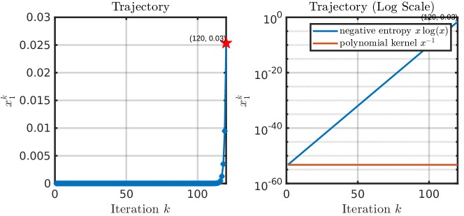
Figure 1: The trajectory plot for $\{x_{1}^{k}\}_{k\in[K]}$ in Example 5 and 6 ($\alpha=1$), with $K=120$ and $\epsilon=0.1$. The initial point is chosen according to the negative entropy kernel scenario.

From the example involving negative entropy, it becomes clear that constructing the initial point at a distance that exponentially decays with respect to the spurious point is crucial. Later on, we want to provide another artificially constructed example to demonstrate the importance of the kernel function’s growth condition in determining the necessary distance between the initial point and the spurious point to trigger a finite step trap. Essentially, the challenge of falling into a finite step trap varies significantly across different kernel functions.

Example 6 (Polynomial kernel).

We still consider the convex counter-example presented in Example 3 with a kernel function as $\varphi(x)=\frac{1}{\alpha}x^{-a}$ where $\alpha>0$. For any $K\in{\mathbb{N}}$ and $\epsilon>0$, we construct the initial point $\bm{x}^{0}$ as follows:

$$\bm{x}^{0}_{1}=\min\left\{\left(\frac{2}{tK+\epsilon^{-(\alpha+1)}}\right)^{\frac{1}{\alpha+1}},\frac{2^{\alpha+1}}{1+2^{\alpha+1}}\right\}$$

and $x^{0}_{2}=1-x^{0}_{1}$. Moreover, for all $k\in[K]$, we apply the standard Bregman gradient descent method as

$$\bm{x}^{k+1} =\arg\min_{\bm{y}}t(-1,0)^{T}\bm{y}+D_{h}(\bm{y},\bm{x}^{k})+\delta_{\Delta_{2}}(\bm{y}).$$

If $\bm{x}^{k}\in{\rm int}(\operatorname{dom}(h))\cap{\cal X}$, we have $\bm{x}^{k+1}\in{\rm{int}}(\operatorname{dom}(h))\cap{\cal X}$ from Lemma 1. We can write down its optimality condition:

$$\left\{\begin{aligned} &-t+\varphi^{\prime}(x_{1}^{k+1})-\varphi^{\prime}(x_{1}^{k})+\mu_{k+1}=0\\ &\varphi^{\prime}(x_{2}^{k+1})-\varphi^{\prime}(x_{2}^{k})+\mu_{k+1}=0\\ &x_{1}^{k+1}+x_{2}^{k+1}=1.\end{aligned}\right.$$

Summing up the above equation from $k=0$ to $k=K-1$, we have

$$\left\{\begin{aligned} &-tK+\varphi^{\prime}(x_{1}^{K})-\varphi^{\prime}(x_{1}^{0})+\sum_{k=1}^{K}\mu_{k+1}=0\\ &\varphi^{\prime}(x_{2}^{K})-\varphi^{\prime}(x_{2}^{0})+\sum_{k=1}^{K}\mu_{k+1}=0.\end{aligned}\right.$$

Since $\varphi^{\prime}(x)=-x^{-\alpha-1}$ and $(\varphi^{\prime})^{-1}(y)=\left(-\frac{1}{y}\right)^{\frac{1}{1+\alpha}}$, we know $\varphi^{\prime}$ is negative on ${\mathbb{R}}_{++}$ and $(\varphi^{\prime})^{-1}$ is monotonically increasing on ${\mathbb{R}}_{-}$. Then, we have

$$-\sum_{k=1}^{K}\mu_{k+1}=\varphi^{\prime}(x_{2}^{K})-\varphi^{\prime}(x_{2}^{0})\leq-\varphi^{\prime}(x_{2}^{0}).$$

Finally, we proceed to bound $x_{1}^{K}$

$$x_{1}^{K} =(\varphi^{\prime})^{-1}\left(\varphi^{\prime}(x_{1}^{0})-\sum_{k=1}^{K}\mu_{k+1}+tK\right)$$

$$\leq(\varphi^{\prime})^{-1}\left(\varphi^{\prime}(x_{1}^{0})-\varphi^{\prime}(1-x_{1}^{0})+tK\right)$$

$$=\left({(x_{1}^{0})^{-\alpha-1}-(1-x_{1}^{0})^{-\alpha-1}-tK}\right)^{\frac{-1}{1+\alpha}}\leq\epsilon.$$

where the first inequality follows from $-\sum_{k=1}^{K}\mu_{k+1}\leq-\varphi^{\prime}(x_{2}^{0})$ and $x_{1}^{0}+x_{2}^{0}=1$ and the last inequality follows from

$$(x_{1}^{0})^{-\alpha-1}-(1-x_{1}^{0})^{-\alpha-1}\geq(2x_{1}^{0})^{-\alpha-1}$$

due to $x_{1}^{0}\leq\frac{2^{\alpha+1}}{1+2^{\alpha+1}}$ and $(2x_{1}^{0})^{-\alpha-1}-tK>0$. For simplicity, we ignore the final constant $\sqrt{2}$.

Remark 6.

From Figure 1, it is evident that despite both kernels facing the challenges outlined in Theorem 3, the nonnegative entropy kernel demonstrates superior performance compared to the polynomial kernel. This advantage can be attributed to the curvature information encapsulated by the inverse mapping of $\nabla h(\bm{x})$. Specifically, when $h(\bm{x})=\bm{x}\log(\bm{x})$, $\nabla^{-1}h(\bm{x})$ exhibits exponential growth behavior, enabling each iteration to escape the unfavorable point by at least doubling the distance from it.

6 Closing remark

In this paper, we conduct a thorough investigation into a fundamental question: Does the equivalence (Q) hold for Bregman divergence-based algorithms, such as mirror descent? Initially, we unify all existing stationarity measures and extend their definitions to the whole domain of kernels. This extension enables us to accommodate widely adopted non-gradient Lipschitz kernels. It is worth noting that prior to our work, the existing stationarity measures are not even well-defined at the boundaries of the kernel functions’ domains. Subsequently, we establish the continuity property of the newly developed stationarity measure and demonstrate that this measure equaling zero is necessary for stationarity. Next, we unveil a surprising result in our paper by disproving the sufficiency direction of the equivalence (Q): A stationarity measure equaling zero can still imply non-stationary points (i.e., spurious stationary points). More significantly, building on this surprising result, we present a hardness result for a class of Bregman divergence-based proximal methods, as illustrated in Algorithm 1. That is, when the algorithm initializes near the spurious stationary point, it’s impossible to get rid of spurious stationary points within finite steps. Ultimately, our in-depth investigation raises an open question:

How to escape from spurious stationary points in Bregman divergence-based proximal algorithms?

To address this question, our paper suggests one possible direction: If we can identify a stationarity measure that meets the equivalence (Q), it might offer new principles for algorithm design to eliminate undesirable points. It is important to note that the hardness result of Theorem 3 is algorithm-dependent. The possibility of addressing this question through algorithmic manner remains unanswered.

The appendix is structured as follows. Firstly, in Appendix A, we present some basic definitions essential for our subsequent discussions. Following that, in Appendix B, we offer an exhaustive verification of Assumption 2 (iv). In Appendix C, we give all proof details of the well-posedness of Algorithm 1 we study in this paper. In Appendix D, we furnish the omitted proofs from the main body to establish the continuity of extended stationarity measure.

Appendix A Supplementary definitions

We begin by revisiting two types of subgradients for convex functions, crucial for analyzing the optimality condition.

Definition 6 (Subgradients of convex functions).

Rockafellar and Wets, (2009, Definition 8.3)) For a convex function $l:{\mathbb{R}}^{n}\to\overline{{\mathbb{R}}}$, we define the subgradient at the point $\overline{\bm{x}}$ by

$$\partial l(\overline{\bm{x}})\coloneqq\left\{\bm{v}\in{\mathbb{R}}^{n}:l(\bm{x})-l(\overline{\bm{x}})\geq\bm{v}^{\top}(\bm{x}-\bar{\bm{x}}),\,\textrm{for all }\bm{x}\in\operatorname{dom}(l)\right\},$$

and the horizon subgradient at the point $\overline{\bm{x}}$ by

$$\partial^{\infty}l(\overline{\bm{x}})\coloneqq\left\{\bm{v}\in{\mathbb{R}}^{n}:\lambda^{k}\bm{v}^{k}\to\bm{v}\text{ with }\lambda^{k}\to 0^{+},\bm{v}^{k}\in\partial l(\bm{x}^{k}),\text{ and }\bm{x}^{k}\to\overline{\bm{x}}\right\}.$$

Then, we introduce the normal cone to handle the convex constraint.

Definition 7 (Normal cone of convex sets).

(Rockafellar and Wets,, 2009, Theorem 6.9)) For a convex set ${\cal D}\subseteq{\mathbb{R}}^{n}$, we define the normal cone at the point $\overline{\bm{x}}\in{\cal D}$ via

$${\cal N}_{{\cal D}}(\overline{\bm{x}})\coloneqq\left\{\bm{v}\in{\mathbb{R}}^{n}:\bm{v}^{\top}(\bm{x}-\overline{\bm{x}})\leq 0,\textrm{ for all }\bm{x}\in{\cal D}\right\}.$$

For more properties of $\partial l$, $\partial^{\infty}l$, and ${\cal N}_{{\cal D}}$, we refer interested readers to (Rockafellar and Wets,, 2009, Chapter 8).

Let us revisit the three-point identity for Bregman divergence, as outlined in Lemma 3.1 of Chen and Teboulle, (1993), i.e.,

$$D_{\varphi}(z,x)+D_{\varphi}(x,y)-D_{\varphi}(z,y)=(z-x)\cdot(\varphi^{\prime}(y)-\varphi^{\prime}(x)),\textrm{ for all }x,y,z\in\operatorname{dom}(\varphi).$$

Since the strict convexity of $\varphi$ implies the strict monotonic increase of $\varphi^{\prime}$, the following fact holds.

Fact 1.

For a strictly convex function $\varphi$, the following statements hold:

1. If $z\leq x\leq y$, then $D_{\varphi}(z,x)\leq D_{\varphi}(z,y)$.

2. If $z\leq x\leq y$, then $D_{\varphi}(x,y)\leq D_{\varphi}(z,y)$.

Next, we introduce the notion of the supercoercive property, commonly employed to ensure the well-posedness of the BPG algorithm; see Bauschke et al., (2017); Bolte et al., (2018).

Definition 8 (Supercoercive property).

Given a function $q:\mathbb{R}^{n}\to\overline{\mathbb{R}}$, we say that $q$ is supercoercive if for all sequences $\{x^{k}\}_{k\in\mathbb{N}}$ such that $\|\bm{x}^{k}\|\to\infty$, it holds that

$$\lim\limits_{k\to\infty}\frac{q(\bm{x}^{k})}{\|\bm{x}^{k}\|}\to+\infty.$$

Appendix B Verification of Assumption 2 (iv)

In this subsection, we aim to identify the condition for Assumption 2 to hold.

1. When $\text{dom}(\phi)$ is open, e.g., $\phi(x)=1/x$, to ensure the well-posedness of the Bregman proximal-type algorithms, we should invoke the compactness of $\mathcal{X}$ as stated in Assumption 2 since the condition (2.1) typically fails. Such a supplement is also made in classical Bregman literature; see condition (i) in (Bauschke et al.,, 2017, Lemma 2).

2. Even without $\mathcal{X}$ being compact, the closeness of $\text{dom}(\phi)$ and the supercoercivity of local update model is able to ensure that Assumption 2 (iv) is met, under Assumptions 1 and 2 (i)–(iii), see Proposition 6 for further details.

Proposition 6.

Suppose that $\text{dom}(\phi)$ is closed. The following hold:

1. If the surrogate model takes the form $\gamma(\bm{y};\bm{x})=f(\bm{x})+\nabla f(\bm{x})^{\top}(\bm{y}-\bm{x})$ and $h+tg$ is supercoercive for all $t>0$, then Assumption 2 (iv) is satisfied.

2. If the surrogate model takes the form $\gamma(\bm{y};\bm{x})=f(\bm{y})$ and $h+tF$ is supercoercive for all $t>0$, then Assumption 2 (iv) is satisfied.

3. If the surrogate model takes the form $\gamma(\bm{y};\bm{x})=f(\bm{x})+\nabla f(\bm{x})^{\top}(\bm{y}-\bm{x})+\frac{1}{2}(\bm{y}-\bm{x})^{\top}\nabla^{2}f(\bm{x})(\bm{y}-\bm{x})$, $h+tg$ is supercoercive for all $t>0$, and $f$ is a convex function, then Assumption 2 (iv) holds.

Remark 7.

Regarding (iii), the convexity condition for $f$ is also posited in Doikov and Nesterov, (2023).

Proof.

Case (i):

To justify that Assumption 2 (iv) is satisfied, we proceed to prove a stronger counterpart, i.e.,

$$\lim\limits_{k\to\infty}\frac{\gamma(\bm{y}^{k};\bm{x}^{k})+g(\bm{y}^{k})+\frac{1}{t}D_{h}(\bm{y}^{k},\bm{x}^{k})}{\|\bm{y}_{k}\|}=+\infty.$$

When $\|\bm{y}^{k}\|\to\infty$, $\bm{x}^{k}\to\overline{\bm{x}}$, and continuity of $\nabla f$, we have

$$\lim\limits_{k\to\infty}\frac{\gamma(\bm{y}^{k};\bm{x}^{k})}{\|\bm{y}^{k}\|}=\nabla f(\overline{\bm{x}})^{\top}\lim\limits_{k\to\infty}\frac{\bm{y}^{k}}{\|\bm{y}^{k}\|}<+\infty.$$

Subsequently, it remains to show

$$\lim\limits_{k\to\infty}\frac{\frac{1}{t}D_{h}(\bm{y}^{k},\bm{x}^{k})+g(\bm{y}^{k})}{\|\bm{y}^{k}\|}=+\infty.$$

To do so, we consider the interior coordinates and boundary coordinates separately. Recall that ${\cal B}(\bar{\bm{x}})=\{b\in[n]:\overline{x}_{b}\in\operatorname{bd}(\operatorname{dom}(\varphi))\}$ and ${\cal I}(\bar{\bm{x}})=\{i\in[n]:\overline{x}_{i}\in{\rm int}(\operatorname{dom}(\varphi))\}$. Without loss of generality (WLOG), we assume that $\text{dom}(\varphi)=[a,b]$.

1. For all $i\in{\cal I}(\bar{\bm{x}})$, we have $\lim\limits_{k\to\infty}|\varphi^{\prime}(x_{i}^{k})|=|\varphi^{\prime}(\bar{x}_{i})|<\infty$ due to the continuous differentiability of $\varphi$. Then, we have

   $$\lim\limits_{k\to\infty}\frac{D_{\varphi}(y^{k}_{i},x^{k}_{i})}{\|\bm{y}^{k}\|} \,=\lim\limits_{k\to\infty}\frac{\varphi(y_{i}^{k})-\varphi(x_{i}^{k})-\varphi^{\prime}(x_{i}^{k})(y_{i}^{k}-x_{i}^{k})}{\|\bm{y}^{k}\|},$$

   $$\,=\lim\limits_{k\to\infty}\frac{\varphi(y_{i}^{k})}{\|\bm{y}^{k}\|}-\varphi^{\prime}(\bar{x}_{i})\cdot\lim\limits_{k\to\infty}\frac{y_{i}^{k}}{\|\bm{y}^{k}\|},\quad\forall i\in{\cal I}(\bar{\bm{x}}),$$ (B.1)

   where the first equality follows from the definition of $D_{\varphi}$ and the second equality is due to the finiteness of $\varphi(\bar{x}_{i})$ and $\bar{x}_{i}$.

2. For all $b\in{\cal B}(\bar{\bm{x}})$, we may assume WLOG that $\bar{x}_{b}=a$. As $\lim_{k\to\infty}x_{b}^{k}=\bar{x}_{b}=a$, we have $x_{b}^{k}<x_{b}^{0}$ for sufficiently large $k$. Then, we try to give a lower bound on $D_{\varphi}(y^{k}_{b},x^{k}_{b})$ and analyze its limit for all $b\in{\cal B}(\bar{\bm{x}})$.

   If $y_{b}^{k}\leq x_{b}^{0}$, then we have $D_{\varphi}(y^{k}_{b},x^{0}_{b})\leq D_{\varphi}(a,x^{0}_{b})$ due to Fact 1 (ii) and $a<y_{b}^{k}\leq x_{b}^{0}$. It follows that

   $$D_{\varphi}(y^{k}_{b},x^{k}_{b})\geq 0\geq D_{\varphi}(y^{k}_{b},x^{0}_{b})-D_{\varphi}(a,x^{0}_{b}),\quad\forall b\in{\cal B}(\bar{\bm{x}}).$$

   Otherwise, we have

   $$D_{\varphi}(y^{k}_{b},x^{k}_{b})\geq D_{\varphi}(y^{k}_{b},x^{0}_{b}),\quad\forall b\in{\cal B}(\bar{\bm{x}}),$$

   due to Fact 1 (i) and $x_{b}^{k}<x_{b}^{0}<y_{b}^{k}$. Consequently, we get

   $$\lim\limits_{k\to\infty}\frac{D_{\varphi}(y^{k}_{b},x^{k}_{b})}{\|\bm{y}^{k}\|}\geq\lim\limits_{k\to\infty}\frac{D_{\varphi}(y^{k}_{b},x^{0}_{b})}{\|\bm{y}^{k}\|}=\lim\limits_{k\to\infty}\frac{\varphi(y^{k}_{b})-\varphi^{\prime}(x^{0}_{b})y^{k}_{b}}{\|\bm{y}^{k}\|},\quad\forall b\in{\cal B}(\bar{\bm{x}}),$$ (B.2)

   where the first inequality follows from the finiteness of $D_{\varphi}(a,x^{0}_{b})$.

Together ((a)) and (B.2), we have

$$\lim\limits_{k\to\infty}\frac{\frac{1}{t}D_{h}(\bm{y}^{k},\bm{x}^{k})+g(\bm{y}^{k})}{\|\bm{y}^{k}\|}$$

$$\geq \lim\limits_{k\to\infty}\frac{\frac{1}{t}h(\bm{y}^{k})+g(\bm{y}^{k})}{\|\bm{y}^{k}\|}-\frac{1}{t}\sum_{i\in{\cal I}(\bar{\bm{x}})}\varphi^{\prime}(\bar{x}_{i})\cdot\lim\limits_{k\to\infty}\frac{y_{i}^{k}}{\|\bm{y}^{k}\|}-\frac{1}{t}\sum_{b\in{\cal B}(\bar{\bm{x}})}\varphi^{\prime}(x_{b}^{0})\cdot\lim\limits_{k\to\infty}\frac{y_{b}^{k}}{\|\bm{y}^{k}\|}=+\infty,$$

where the equality holds since $h+tf$ is supercoercive for all $t>0$ and the finiteness of $\varphi^{\prime}(x_{b}^{0})$ and $\varphi^{\prime}(\bar{x}_{i})$ for all $b\in{\cal B}(\bar{\bm{x}})$ and $i\in{\cal I}(\bar{\bm{x}})$. This completes the proof of case (i).

Case (ii): The ideas of the proof of case (ii) are similar to those of case (i). We just need to replace $g$ with $F$.

Case (iii): Given the convexity of $f$, we find that $(\bm{y}-\bm{x})^{\top}\nabla^{2}f(\bm{x})(\bm{y}-\bm{x})\geq 0$ for any $\bm{y}\in{\mathbb{R}}^{n}$. Thus, it suffices to show

$$\lim\limits_{k\to\infty}{f(\bm{x}^{k})+\nabla f(\bm{x}^{k})^{T}(\bm{y}^{k}-\bm{x}^{k})+g(\bm{y}^{k})+\frac{1}{t}D_{h}(\bm{y}^{k},\bm{x}^{k})}=+\infty,$$

which reduces to the case (i). We complete the proof. ∎

Appendix C Well-posedness of algorithms

To start with, we prove the existence of the extended mapping $\overline{T}_{\gamma}^{t}$.

Lemma 2 (Existence).

For all $\bm{x}\in{\cal X}$, we have

$$\operatorname{argmin}\limits_{\bm{y}\in{\cal X}}\ G^{t}_{\gamma}(\bm{y};\bm{x})\neq\varnothing.$$

Proof.

To ensure the existence of the optimal solution, it suffices to show that, for some constant $c\in{\mathbb{R}}$, the level set $\{\bm{y}\in{\cal X}:G^{t}_{\gamma}(\bm{y};\bm{x})\leq c\}$ is compact for any $\bm{x}\in{\cal X}$. At first, from (Rockafellar and Wets,, 2009, Theorem 1.6), we know this level set is closed due to the lower semicontinuity of $:G^{t}_{\gamma}(\cdot,\bm{x})$ for any $\bm{x}\in{\cal X}$.

Next, our task is to show the set $\{\bm{y}\in{\cal X}:G^{t}_{\gamma}(\bm{y};\bm{x})\leq c\}$ is bounded. We consider two cases separately:

1. If $\bm{x}\in{\rm int}(\operatorname{dom}(h))\cap{\cal X}$, the boundedness of the set $\{\bm{y}\in{\cal X}:G^{t}_{\gamma}(\bm{y};\bm{x})\leq c\}$ is from Assumption 2 (iv), as the coerciveness can imply one non-empty bounded level set.

2. If $\bm{x}\in\operatorname{bd}(\operatorname{dom}(h))\cap{\cal X}$, it suffices to show the coerciveness of $G^{t}_{\gamma}(\cdot;\bm{x})$. That is, if we consider an arbitrary sequence $\{\bm{y}^{k}\}\subseteq{\cal X}$ with $\|\bm{y}^{k}\|\to+\infty$, we have $G^{t}_{\gamma}(\bm{y}^{k};\bm{x})\to+\infty$.

   WLOG, we can assume that $\bm{y}^{k}_{{\cal B}(\bm{x})}\equiv\bm{x}_{{\cal B}(\bm{x})}$; otherwise, $G^{t}_{\gamma}(\bm{y}^{k};\bm{x})=+\infty$, for any $k\in{\mathbb{N}}$. Then, we pick up an interior point $\bm{x}^{{\rm int}}\in{\rm int}(\operatorname{dom}(h))\cap{\cal X}$ and construct three sequences $\{{\bm{x}}^{k}\}_{k\in{\mathbb{N}}}$, $\{\tilde{\bm{y}}^{k}\}_{k\in{\mathbb{N}}}$ and $\{\tilde{\bm{x}}^{k}\}_{k\in{\mathbb{N}}}$ satisfying

   $$\bm{x}^{k}\to\bm{x}\text{ with }{\cal B}(\bm{x}^{k})={\cal B}(\bm{x}),\forall k\in{\mathbb{N}}$$

   $$\tilde{\bm{y}}^{k}=(1-\theta_{k})\bm{y}^{k}+\theta_{k}\bm{x}^{{\rm int}},\forall k\in{\mathbb{N}},$$

   $$\tilde{\bm{x}}^{k}=(1-\theta_{k})\bm{x}^{k}+\theta_{k}\bm{x}^{{\rm int}},\,\forall k\in{\mathbb{N}},$$

   where $\theta_{k}\in(0,1)$ and $\theta_{k}\to 0$. Then, it is trivial to conclude that $\|\tilde{\bm{y}}^{k}\|\to+\infty$ and $\tilde{\bm{x}}^{k}\to\bm{x}$. Moreover, due to $\tilde{\bm{y}}^{k}_{{\cal B}(\bm{x})}=\tilde{\bm{x}}^{k}_{{\cal B}(\bm{x})},\forall k\in{\mathbb{N}}$, we get

   $$\gamma(\tilde{\bm{y}}^{k};\tilde{\bm{x}}^{k})+g(\tilde{\bm{y}}^{k})+\frac{1}{t}D_{h}(\tilde{\bm{y}}^{k},\tilde{\bm{x}}^{k})=\gamma(\tilde{\bm{y}}^{k};\tilde{\bm{x}}^{k})+g(\tilde{\bm{y}}^{k})+\frac{1}{t}\sum_{i\in{\cal I}(\bm{x})}D_{\varphi}(\tilde{y}^{k}_{i},\tilde{x}^{k}_{i}).$$

   By the continuity of the mappings $\gamma(\cdot),g(\cdot)$, and $D_{\phi}(\cdot,\cdot)$, there exists a sufficiently small $\theta_{k}>0$ such that

   $$\left|\gamma(\tilde{\bm{y}}^{k};\tilde{\bm{x}}^{k})+g(\tilde{\bm{y}}^{k})+\frac{1}{t}D_{h}(\tilde{\bm{y}}^{k},\tilde{\bm{x}}^{k})-G^{t}_{\gamma}(\bm{y}^{k};\bm{x})\right|\leq 1.$$

   From Assumption 2 (iv), we know $\gamma(\tilde{\bm{y}}^{k};\tilde{\bm{x}}^{k})+g(\tilde{\bm{y}}^{k})+\frac{1}{t}D_{h}(\tilde{\bm{y}}^{k},\tilde{\bm{x}}^{k})\to+\infty$. Thus, we can conclude that $G^{t}_{\gamma}(\bm{y}^{k};\bm{x})\to+\infty$.

∎

C.1 Proof of Lemma 1

Proof.

We prove this by contradiction. Suppose that $\bm{x}\in{\rm{int}}(\operatorname{dom}(h))$ and $T^{t}_{\gamma}(\bm{x})\notin{\rm{int}}(\operatorname{dom}(h))$. Then, can select an interior point $\mathbf{x}^{\text{int}}\in\text{int}(\text{dom}(h))\cap\mathcal{X}$, where its distance from $T^{t}_{\gamma}(\mathbf{x})$ is bounded. Subsequently, we construct an intermediate point as

$$\bm{x}^{\theta}\coloneqq\theta\bm{x}^{{\rm{int}}}+(1-\theta)T^{t}_{\gamma}(\bm{x}),$$

and an univariate function as

$$\phi(\theta)\coloneqq\gamma\left(\bm{x}^{\theta};\bm{x}\right)+\frac{1}{t}D_{h}\left(\bm{x}^{\theta},\bm{x}\right)+g\left(\bm{x}^{\theta}\right),$$

where $\theta\in(0,1]$.

Our strategy is to show that

$$\lim_{\theta\to 0_{+}}\frac{\phi(\theta)-\phi(0)}{\theta}=-\infty$$

holds . Then, it is sufficient to demonstrate that there exists a constant $\theta\in(0,1)$ such that $\phi(\theta)-\phi(0)$, thereby contradicting the definition of $T^{t}_{\gamma}(\bm{x})$.

Now, we focus on the decomposition of $\phi(\theta)-\phi(0)$ as below:

$$\ \phi(\theta)-\phi(0)$$

$$= \ \gamma\left(\bm{x}^{\theta};\bm{x}\right)-\gamma(T^{t}_{\gamma}(\bm{x});\bm{x})+g\left(\bm{x}^{\theta}\right)-g(T^{t}_{\gamma}(\bm{x}))+\frac{1}{t}\left(D_{h}\left(\bm{x}^{\theta},\bm{x}\right)-D_{h}(T^{t}_{\gamma}(\bm{x}),\bm{x})\right)$$

$$= \ \left[\gamma\left(\bm{x}^{\theta};\bm{x}\right)-\gamma(T^{t}_{\gamma}(\bm{x});\bm{x})\right]+\left[g\left(\bm{x}^{\theta}\right)-g(T^{t}_{\gamma}(\bm{x}))\right]+\left[\frac{1}{t}\sum_{j=1}^{n}\left(\varphi\left(x^{\theta}_{j}\right)-\varphi\left(T^{t}_{\gamma}(\bm{x})_{j}\right)\right)\right]$$

$$\ \left[-\frac{\theta}{t}\sum_{j=1}^{n}\varphi^{\prime}(x_{j})\left(x^{{\rm{int}}}_{j}-T^{t}_{\gamma}(\bm{x})_{j}\right)\right].$$

Then, we address each component individually.

1. Due to the differentiability of $\gamma(\cdot,\bm{x})$ at the point $\bm{x}$ (see Assumption 2 (ii)), there exists a sufficient small $\theta$ such that

   $$\left|\frac{\gamma\left(\bm{x}^{\theta};\bm{x}\right)-\gamma\left(T^{t}_{\gamma}(\bm{x});\bm{x}\right)}{\theta}\right|\leq\mathcal{O}(1).$$

2. Given the local Lipschitz continuity of $g$ on $\mathcal{X}$, there also exists a sufficiently small $\theta$ (i.e., you can certainly choose the same $\theta$ to satisfy both (i) and (ii)) such that

   $$\left|\frac{g\left(\bm{x}^{\theta}\right)-g(T^{t}_{\gamma}(\bm{x}))}{\theta}\right|\leq\mathcal{O}(1).$$

3. By Mean Value Theorem, we have

   $$\sum_{j=1}^{n}\frac{\varphi\left(x^{\theta}_{j}\right)-\varphi\left(T^{t}_{\gamma}(\bm{x})_{j}\right)}{\theta}=\sum_{j=1}^{n}\varphi^{\prime}\left(z^{\theta}_{j}\right)\cdot\left(x^{{\rm{int}}}_{j}-T^{t}_{\gamma}(\bm{x})_{j}\right),$$

   where $z^{\theta}_{j}$ is in the interval between $x^{\theta}_{j}$ and $T^{t}_{\gamma}(\bm{x})_{j}$ for all $j\in[n]$. When $\theta\to 0_{+}$, the term $(x^{{\rm{int}}}_{j}-T^{t}_{\gamma}(\bm{x})_{j})$ is always bounded. Moreover, we have $z^{\theta}_{b}\to T^{t}_{\gamma}(\bm{x})_{b}$ when $\theta\to 0^{+}$. Thus, the key lies in the boundedness of $\varphi^{\prime}(T^{t}_{\gamma}(\bm{x})_{j}))$ for all $j\in[n]$.

   We will discuss the interior coordinates and boundary coordinate of $T^{t}_{\gamma}(\bm{x})$ separately.

   1. For all $i\in{\cal I}(T^{t}_{\gamma}(\bm{x}))$, we know that $T^{t}_{\gamma}(\mathbf{x})_{i}\in\text{int}(\text{dom}(\varphi))$, and therefore $\varphi^{\prime}(T^{t}_{\gamma}(\mathbf{x})_{i})$ is bounded due to the continuity of $\varphi^{\prime}$.

   2. For all $b\in{\cal B}(T^{t}_{\gamma}(\bm{x}))$, we have $T^{t}_{\gamma}(\bm{x})_{b}\in\rm{bd}(\operatorname{dom}(\varphi))$ and thus $|\varphi^{\prime}(T^{t}_{\gamma}(\bm{x})_{b})|=+\infty$ from Definition 1 (ii). WLOG, we can assume that $\textrm{cl}(\text{dom}(\varphi))=[a,c]$ and $T^{t}_{\gamma}(\bm{x})_{b}=a$. Moreover, as $\varphi^{\prime}$ is strictly increasing by the strict convexity of $\varphi$, we have $\varphi^{\prime}(T^{t}_{\gamma}(\bm{x})_{b})=-\infty$. Together with the fact $x^{{\rm{int}}}_{b}-T^{t}_{\gamma}(\bm{x})_{b}>0$, we have

      $$\lim_{\theta\to 0_{+}}\varphi^{\prime}\left(z^{\theta}_{b}\right)\cdot\left(x^{{\rm{int}}}_{b}-T^{t}_{\gamma}(\bm{x})_{b}\right)=-\infty.$$

4. The final term is constant w.r.t. $\theta$ and thus bounded for sure.

Putting all the pieces together, we conclude the proof. ∎

Appendix D Proof of continuity of extended stationarity measure

To begin, we introduce two technical lemmas essential for proving Proposition 1.

Lemma 3.

Suppose the sequence $\{\bm{x}^{k}\}_{k\in{\mathbb{N}}}\subseteq{\rm int}(\operatorname{dom}(h))\cap{\cal X}$ is bounded, and the sequence $\{T^{t}_{\gamma}(\bm{x}^{k})\}_{k\in{\mathbb{N}}}$ converges to $\bm{x}^{*}\in{\cal X}$. We define a sequence $\{\bm{d}^{k+1}\}_{k\in{\mathbb{N}}}$ satisfying

$$\nabla\gamma\left(T^{t}_{\gamma}(\bm{x}^{k});\bm{x}^{k}\right)+\bm{d}^{k+1}+\frac{1}{t}\left(\nabla h\left(T^{t}_{\gamma}(\bm{x}^{k})\right)-\nabla h(\bm{x}^{k})\right)={\mathbf{0}}\text{ and }\bm{d}^{k+1}\in\partial g\left(T^{t}_{\gamma}(\bm{x}^{k})\right).$$ (D.1)

Then, the sequence $\{\bm{d}^{k+1}\}_{k\in{\mathbb{N}}}$ is bounded.

Proof.

We prove the boundedness of $\{\bm{d}^{k+1}\}_{k\in{\mathbb{N}}}$ by contradiction. Suppose that the sequence $\{\bm{d}^{k+1}\}_{k\in{\mathbb{N}}}$ is not bounded. Then, there must exist a subsequence that diverges. WLOG, we can assume that $\|\bm{d}^{k+1}\|\to\infty$ and ${\bm{d}^{k+1}}/{\|\bm{d}^{k+1}\|}\to\bm{d}^{*}$ for some $\bm{d}^{*}$. Due to Definition 6 and $T^{t}_{\gamma}(\bm{x}^{k})\to\bm{x}^{*}$, we have $\bm{d}^{*}\in\partial^{\infty}g(\bm{x}^{*})$. Moreover, owing to the convexity and continuity of the function $g$, we can apply Rockafellar and Wets, (2009, Proposition 8.12) to get $\partial^{\infty}g(\bm{x}^{*})={\cal N}_{{\cal X}}(\bm{x}^{*})$ and hence we have

$$(\bm{x}^{*}-\bm{x})^{\top}\bm{d}^{*}\geq 0\text{ for all }\bm{x}\in{\cal X}.$$ (D.2)

In view of (D.2), we consider the following two scenarios separately:

1. $(\bm{x}^{*}-\bm{x})^{\top}\bm{d}^{*}=0\text{ for all }\bm{x}\in{\cal X};$

2. There exists some $\bm{x}\in{\cal X}$ such that $(\bm{x}^{*}-\bm{x})^{\top}\bm{d}^{*}>0.$

Scenarios (i): For all $k\in{\mathbb{N}}$, we have

$$(T^{t}_{\gamma}(\bm{x}^{k})-\bm{x}^{k})^{\top}\bm{d}^{*}=0,$$ (D.3)

by substituting $\bm{x}=\bm{x}^{k}$ and $\bm{x}=T^{t}_{\gamma}(\bm{x}^{k})$ in (D.2), and summing them.

From (D.3), we have

$$\varphi^{\prime}\left(T^{t}_{\gamma}(\bm{x}^{k})_{i}\right)-\varphi^{\prime}(x^{k}_{i})=-t\left(\nabla_{i}\gamma(T^{t}_{\gamma}(\bm{x}^{k});\bm{x}^{k})+d^{k+1}_{i}\right),\,\forall i\in[n].$$ (D.4)

Next, we want to argue that the left-hand side of (D.4) will go to infinity, which will contradict with (D.3).

Given the boundedness of the sequence $\{\bm{x}^{k}\}_{k\in\mathbb{N}}$ and $\{T^{t}_{\gamma}(\bm{x}^{k})\}_{k\in{\mathbb{N}}}\to\bm{x}^{*}$, it follows from the joint continuity property of $\nabla\gamma(\cdot;\cdot)$, as stated in Assumption 2 (i), that $\{\nabla_{i}\gamma(T^{t}_{\gamma}(\mathbf{x}^{k});\mathbf{x}^{k})\}_{k\in\mathbb{N}}$ is also bounded. We proceed to discuss the term $d^{k+1}_{i}$ for all $i\in[n]$. Let ${\cal I}^{+}\coloneqq\{i\in[n]:d^{*}_{i}>0\}$ and ${\cal I}^{-}\coloneqq\{i\in[n]:d^{*}_{i}<0\}$. Thus, we have $d^{k+1}_{i}\to+\infty$ (resp. $d^{k+1}_{i}\to-\infty$) by $d^{k+1}_{i}/\|\bm{d}^{k+1}\|\to d^{*}_{i}$, for all $i\in{\cal I}^{+}$ (resp. ${\cal I}^{-}$). Hence, the equation (D.4) yields

$$\varphi^{\prime}\left(T^{t}_{\gamma}(\bm{x}^{k})_{i}\right)-\varphi^{\prime}(x^{k}_{i})\to-\infty\text{ (resp. }+\infty\text{) for }i\in{\cal I}^{+}\text{ (resp. }i\in{\cal I}^{-}\text{)}.$$

Moreover, since $\varphi^{\prime}$ is strictly increasing by the strict convexity of $\varphi$, for sufficiently large $k$, we have

$$T^{t}_{\gamma}(\bm{x}^{k})_{i}<x_{i}^{k}\text{ for }i\in{\cal I}^{+}\text{ and }T^{t}_{\gamma}(\bm{x}^{k})_{i}>x_{i}^{k}\text{ for }i\in{\cal I}^{-}.$$

Consequently, we get

$$(T^{t}_{\gamma}(\bm{x}^{k})-\bm{x}^{k})^{\top}\bm{d}^{*}<0\text{ for sufficiently large }k,$$

which contradicts (D.3).

Scenarios (ii): There must exists a point $x\in{\cal X}$ and a positive constant $\alpha>0$ such that $(\bm{x}^{*}-\bm{x})^{\top}\bm{d}^{*}\geq\alpha$. Additionally, we can select some $\bm{x}^{{\rm int}}\in{\rm int}(\operatorname{dom}(h))\cap{\cal X}$, which is sufficiently close to $\bm{x}$ such that $(\bm{x}^{{\rm int}}-x)^{T}\bm{d}^{*}\leq\frac{\alpha}{2}$. Therefore, we have

$$(\bm{x}^{*}-\bm{x}^{{\rm int}})^{T}\bm{d}^{*}=\lim_{k\to\infty}(T^{t}_{\gamma}(\bm{x}^{k})-\bm{x}^{{\rm int}})^{T}\frac{\bm{d}^{k+1}}{\|\bm{d}^{k+1}\|}\geq\frac{\alpha}{2}.$$

where the first equality follows from $T^{t}_{\gamma}(\bm{x}^{k})\to\bm{x}^{*}$ and the definition of $\bm{d}^{*}$. Then, for sufficiently large $k$, we have

$$(T^{t}_{\gamma}(\bm{x}^{k})-\bm{x}^{{\rm int}})^{T}\bm{d}^{k+1}\geq\frac{\alpha}{2}\|\bm{d}^{k+1}\|.$$ (D.5)

Furthermore, by multiplying (D.1) by $T^{t}_{\gamma}(\bm{x}^{k})-\bm{x}^{{\rm int}}$, we obtain

$$(T^{t}_{\gamma}(\bm{x}^{k})-\bm{x}^{{\rm int}})^{\top}\left[\nabla\gamma\left(T^{t}_{\gamma}(\bm{x}^{k});\bm{x}^{k}\right)+\bm{d}^{k+1}+\frac{1}{t}\left(\nabla h(T^{t}_{\gamma}(\bm{x}^{k}))-\nabla h(\bm{x}^{k})\right)\right]=0.$$

It follows that

$$(T^{t}_{\gamma}(\bm{x}^{k})-\bm{x}^{{\rm int}})^{\top}\left(\nabla h(T^{t}_{\gamma}(\bm{x}^{k}))-\nabla h(\bm{x}^{k})\right)$$ (D.6)

$$= -(T^{t}_{\gamma}(\bm{x}^{k})-\bm{x}^{{\rm int}})^{T}\bm{d}^{k+1}-(T^{t}_{\gamma}(\bm{x}^{k})-\bm{x}^{{\rm int}})^{T}\nabla\gamma\left(T^{t}_{\gamma}(\bm{x}^{k});\bm{x}^{k}\right)$$

$$\leq -\frac{\alpha}{2}\|\bm{d}^{k+1}\|^{2}-(T^{t}_{\gamma}(\bm{x}^{k})-\bm{x}^{{\rm int}})^{T}\nabla\gamma\left(T^{t}_{\gamma}(\bm{x}^{k});\bm{x}^{k}\right)\to-\infty,$$

where the first inequality is due to (D.5), and the last limit follows from the boundedness of $\{\nabla\gamma(T^{t}_{\gamma}(\bm{x}^{k});\bm{x}^{k})\}_{k\in{\mathbb{N}}}$ and $\|\bm{d}^{k+1}\|\to\infty$.

We now utilize (D.6) to establish the contradiction. The key proof idea follows from the one in Lemma 1. For all $k\in{\mathbb{N}}$, we construct a sequence of intermediate points as

$$\bm{x}^{\theta,k}\coloneqq\theta\bm{x}^{{\rm{int}}}+(1-\theta)T^{t}_{\gamma}(\bm{x}^{k}),$$

and a sequence of univariate functions as

$$\phi_{k}(\theta)\coloneqq\gamma\left(\bm{x}^{\theta,k};\bm{x}\right)+\frac{1}{t}D_{h}\left(\bm{x}^{\theta,k},\bm{x}\right)+g\left(\bm{x}^{\theta,k}\right),$$

where $\theta\in(0,1]$. By the definition of $T^{t}_{\gamma}(\bm{x}^{k})$, we have $\phi_{k}(0)=\min_{\theta\in[0,1]}\phi_{k}(\theta)$ for $k\in{\mathbb{N}}$. Then, our strategy is to show that for sufficiently large $k$

$$\lim_{\theta\to 0_{+}}\frac{\phi_{k}(\theta)-\phi_{k}(0)}{\theta}<0,$$

and thus yields a contradiction. By Mean Value Theorem, we have

$$\frac{\phi_{k}(\theta)-\phi_{k}(0)}{\theta}$$

$$= \frac{\gamma\left(\bm{x}^{\theta,k};\bm{x}\right)-\gamma\left(T^{t}_{\gamma}(\bm{x}^{\theta,k});\bm{x}\right)}{\theta}+\frac{1}{t}(T^{t}_{\gamma}(\bm{x}^{k})-\bm{x}^{{\rm int}})^{\top}\left(\nabla h(\bm{z}^{\theta,k})-\nabla h(\bm{x}^{k})\right)$$

$$+\frac{g\left(\bm{x}^{\theta,k}\right)-g\left(T^{t}_{\gamma}(\bm{x}^{k})\right)}{\theta},$$ (D.7)

where $\bm{z}^{\theta,k}$ is between $\bm{x}^{\theta,k}$ and $T^{t}_{\gamma}(\bm{x}^{k})$. Owing to the continuous differentiability of $\gamma$ and local Lipschitz continuity of $g$, we know the first and third terms in (D.7) are bounded. From (D.6), as $\theta$ approaches $0_{+}$, the second term tends toward $-\infty$ for sufficiently large $k$. Consequently, we have

$$\lim\limits_{k\to\infty}\lim\limits_{\theta\to 0^{+}}\frac{\phi_{k}(\theta)-\phi_{k}(0)}{\theta}=-\infty,$$

which leads to a contradiction. We complete our proof. ∎

Next, we extend Lemma 3 to a more general case, whose proof techiniques are essentially the same as the one developed in Lemma 3.

Corollary 2.

Suppose that the sequence $\{\bm{x}^{k}\}_{k\in{\mathbb{N}}}\subseteq{\cal X}$ is bounded satisfying ${\cal I}(\bm{x}^{k})\equiv{\cal I}_{0}\subseteq[n]$ and ${\cal B}(\bm{x}^{k})\equiv{\cal B}_{0}$, and the sequence $\{\overline{T}^{t}_{\gamma}(\bm{x}^{k})\}_{k\in{\mathbb{N}}}$ converges to $\bm{x}^{*}\in{\cal X}$. We define a sequence $\{\bm{d}^{k+1}\}_{k\in{\mathbb{N}}}$ satisfying

$$\nabla\gamma(\overline{T}^{t}_{\gamma}(\bm{x}^{k});\bm{x}^{k})+\bm{d}^{k+1}+\bm{p}^{k+1}+\frac{1}{t}\sum_{i\in{\cal I}_{0}}\nabla\left(D_{\varphi}(\overline{T}^{t}_{\gamma}(\bm{x}^{k})_{i},x^{k}_{i})\right)={\mathbf{0}},$$ (D.8)

where $\bm{d}^{k+1}\in\partial g\left(\overline{T}^{t}_{\gamma}(\bm{x}^{k})\right)$ and $\bm{p}^{k+1}\in\partial\delta_{\bm{y}_{{\cal B}_{0}}=\bm{x}^{k}_{{\cal B}_{0}}}\left(\overline{T}^{t}_{\gamma}(\bm{x}^{k})\right)$, for all $k\in{\mathbb{N}}$. Then, the sequence $\{\bm{d}^{k+1}_{{\cal I}_{0}}\}_{k\in{\mathbb{N}}}$ is bounded.

Proof.

WLOG, we assume that $\text{cl}(\text{dom}(\varphi))=[a,c]$ and $\bm{x}^{k}_{{\cal B}_{0}}\equiv\bm{x}^{0}_{{\cal B}_{0}}$ for all $k\in{\mathbb{N}}$. Let $\tilde{g}=g+\delta_{\bm{y}_{{\cal B}_{0}}=\bm{x}^{0}_{{\cal B}_{0}}}$, $\tilde{{\cal X}}={\cal X}\cap\{\bm{y}\in{\cal X}:\bm{y}_{{\cal B}_{0}}=\bm{x}^{0}_{{\cal B}_{0}}\}$, and $\tilde{\bm{d}}^{k+1}=\bm{d}^{k+1}+\bm{p}^{k+1}$. Then, we have

$$\tilde{\bm{d}}^{k+1}_{{\cal B}_{0}}=\bm{d}^{k+1}_{{\cal B}_{0}},\ \tilde{\bm{d}}^{k+1}\in\partial\tilde{g}\left(\overline{T}^{t}_{\gamma}(\bm{x}^{k})\right),\text{ and }\operatorname{dom}(\tilde{g})=\tilde{{\cal X}}.$$

We continue to rewrite (D.8) as

$$\nabla\gamma(\overline{T}^{t}_{\gamma}(\bm{x}^{k});\bm{x}^{k})+\tilde{\bm{d}}^{k+1}+\frac{1}{t}\sum_{i\in{\cal I}_{0}}\nabla\left(D_{\varphi}(\overline{T}^{t}_{\gamma}(\bm{x}^{k})_{i},x^{k}_{i})\right)={\mathbf{0}},$$ (D.9)

where $\tilde{\bm{d}}^{k+1}\in\partial\tilde{g}\left(\overline{T}^{t}_{\gamma}(\bm{x}^{k})\right).$ Due to the boundedness of $\{\overline{T}^{t}_{\gamma}(\bm{x}^{k})\}_{k\in{\mathbb{N}}}$ and $\{\bm{x}^{k}\}_{k\in{\mathbb{N}}}$, and the continuity of $\nabla\gamma$, it follows that the sequence $\{\nabla\gamma(\overline{T}^{t}_{\gamma}(\bm{x}^{k});\bm{x}^{k})\}_{k\in{\mathbb{N}}}$ is bounded. Moreover, we know the sequence $\{\tilde{\bm{d}}^{k+1}_{{\cal B}_{0}}\}_{k\in{\mathbb{N}}}$ is bounded from the boundedness of $\{\overline{T}^{t}_{\gamma}(\bm{x}^{k})\}_{k\in{\mathbb{N}}}$ and (D.9).

We left to show the sequence $\{\bm{d}^{k+1}_{{\cal I}_{0}}\}_{k\in{\mathbb{N}}}$ is bounded. We prove this result by contradiction. Suppose that the sequence $\{\bm{d}^{k+1}_{{\cal I}_{0}}\}_{k\in{\mathbb{N}}}$ is unbounded. Hence, the sequence $\{\tilde{\bm{d}}^{k+1}\}_{k\in{\mathbb{N}}}$ is also unbounded. Then, there must exist a subsequence that diverges. WLOG, we can assume that ${\tilde{\bm{d}}^{k+1}}/{\|\tilde{\bm{d}}^{k+1}\|}\to\overline{\bm{d}}$ for some $\overline{\bm{d}}$. Here, we have $\|\overline{\bm{d}}_{{\cal I}_{0}}\|=1$ and $\overline{\bm{d}}_{{\cal B}_{0}}={\mathbf{0}}$ due to boundedness of $\{\tilde{\bm{d}}^{k+1}_{{\cal B}_{0}}\}_{k\in{\mathbb{N}}}$. Then, the left proof is the same as the one in Lemma 3. We omit the proof details. ∎

Lemma 4.

If the sequence $\{\bm{x}^{k}\}_{k\in{\mathbb{N}}}\subseteq\operatorname{int}(\operatorname{dom}(h))\cap{\cal X}$ is bounded, then the sequence $\{T^{t}_{\gamma}(\bm{x}^{k})\}_{k\in{\mathbb{N}}}$ is also bounded.

Proof.

We prove this result by contradiction. WLOG, we can assume $\bm{x}^{k}\to\overline{\bm{x}}\in{\cal X}$ by the boundedness of $\{\bm{x}^{k}\}_{k\in{\mathbb{N}}}$. From Assumption 2 (iv), we have

$$\lim_{k\to+\infty}\gamma(T^{t}_{\gamma}(\bm{x}^{k}),\bm{x}^{k})+\frac{1}{t}D_{h}(T^{t}_{\gamma}(\bm{x}^{k}),\bm{x}^{k})+g(T^{t}_{\gamma}(\bm{x}^{k}))=+\infty.$$ (D.10)

Moreover, we have

$$\lim_{k\to+\infty}\gamma(\bm{x}^{k};\bm{x}^{k})+\frac{1}{t}D_{h}(\bm{x}^{k},\bm{x}^{k})+g(\bm{x}^{k})=\gamma(\overline{\bm{x}};\overline{\bm{x}})+g(\overline{\bm{x}})=f(\overline{\bm{x}})+g(\overline{\bm{x}})<+\infty,$$

where the first equality is owing to the continuity of $\gamma$ and $g$, the second one is from Assumption 2 (ii), and the last inequality is due to $\overline{\bm{x}}\in{\cal X}$. Then, together with (D.10), for $k$ large enough, it follows that

$$\gamma(T^{t}_{\gamma}(\bm{x}^{k}),\bm{x}^{k})+\frac{1}{t}D_{h}(T^{t}_{\gamma}(\bm{x}^{k}),\bm{x}^{k})+g(T^{t}_{\gamma}(\bm{x}^{k}))>\gamma(\bm{x}^{k},\bm{x}^{k})+\frac{1}{t}D_{h}(\bm{x}^{k},\bm{x}^{k})+g(\bm{x}^{k}),$$

which contradicts with the definition of $T^{t}_{\gamma}(\bm{x}^{k})$. Hence, the sequence $\{T^{t}_{\gamma}(\bm{x}^{k})\}_{k\in{\mathbb{N}}}$ is bounded. ∎

Now, we are ready to give a full proof of Proposition 1.

D.1 Proof of Proposition 1

Proof.

To show that the mapping $\overline{T}^{t}_{\gamma}(\cdot)$ is continuous, it suffices to show that for any sequence $\{\bm{x}^{k}\}_{k\in{\mathbb{N}}}\subseteq{\cal X}$ converging to $\bm{x}\in{\cal X}$, it holds that:

$$\lim\limits_{k\to\infty}\overline{T}^{t}_{\gamma}(\bm{x}^{k})=\overline{T}^{t}_{\gamma}(\bm{x}).$$

To proceed, we consider the following two scenarios sequentially:

1. The sequence $\{\bm{x}^{k}\}_{k\in{\mathbb{N}}}\subseteq\operatorname{int}(\operatorname{dom}(h))\cap{\cal X}$.

2. The sequence $\{\bm{x}^{k}\}_{k\in{\mathbb{N}}}\subseteq\operatorname{cl}(\operatorname{dom}(h))\cap{\cal X}$.

To start with, we consider the simple case (i). Later on, we can extend our proof strategy to consider the general case by considering the interior and boundary coordinates of $\bm{x}$ separately. Then, we can reduce the general case to the simple case considered here.

Scenarios (i): Due to $\overline{T}^{t}_{\gamma}(\cdot)={T}^{t}_{\gamma}(\cdot)$ on ${\rm{int}}(\operatorname{dom}(h))\cap{\cal X}$. It is equivalent to show

$$\overline{T}^{t}_{\gamma}(\bm{x})=\lim\limits_{k\to\infty}{T}^{t}_{\gamma}(\bm{x}^{k}).$$

The remainder of the proof proceeds in two steps. We give a proof sketch here initially.

• Step 1: For the boundary coordinates of $\bm{x}$, we have $\lim_{k\to\infty}{T}^{t}_{\gamma}(\bm{x}^{k})_{{\cal B}(\bm{x})}=\overline{T}^{t}_{\gamma}(\bm{x})_{{\cal B}(\bm{x})}$.

  By Lemma 4, we can pass to a subsequence such that $T^{t}_{\gamma}(\bm{x}^{k})\to\tilde{\bm{x}}\in\operatorname{cl}(\operatorname{dom}(h))$. Then, we have to show $\tilde{\bm{x}}_{{\cal B}(\bm{x})}={\bm{x}}_{{\cal B}(\bm{x})}$ from the definition of $\overline{T}^{t}_{\gamma}$, i.e., $\overline{T}^{t}_{\gamma}(\bm{x})_{{\cal B}(\bm{x})}=\bm{x}_{{\cal B}(\bm{x})}$. We prove this result by contradiction. Our proof strategy essentially follows the one we developed in Lemma 1 and Lemma 3. For all $k\in{\mathbb{N}}$, we construct a sequence of intermediate points as

  $$\bm{x}^{\theta,k}\coloneqq\theta\bm{x}^{k}+(1-\theta)T^{t}_{\gamma}(\bm{x}^{k}),$$

  and a sequence of univariate functions as

  $$\phi_{k}(\theta)\coloneqq\gamma\left(\bm{x}^{\theta,k};\bm{x}\right)+\frac{1}{t}D_{h}\left(\bm{x}^{\theta,k},\bm{x}\right)+g\left(\bm{x}^{\theta,k}\right),$$

  where $\theta\in(0,1]$. Then, we show $\phi_{k}(\theta)<\phi_{k}(0)$ would hold for some $\theta\in(0,1]$ and $k\in{\mathbb{N}}$ if $\tilde{\bm{x}}_{{\cal B}(\bm{x})}\neq\bm{x}_{{\cal B}(\bm{x})}$.

• Step 2: We prove $\tilde{\bm{x}}=\lim_{k\to\infty}T^{t}_{\gamma}(\bm{x}^{k})=\overline{T}^{t}_{\gamma}(\bm{x})$ via the optimality condition.

  For all $k\in{\mathbb{N}}$, from the definition of ${T}^{t}_{\gamma}(\bm{x}^{k})$, we can write down its optimality condition:

  $$\nabla\gamma\left(T^{t}_{\gamma}(\bm{x}^{k});\bm{x}^{k}\right)+\frac{1}{t}\left(\nabla h(T^{t}_{\gamma}(\bm{x}^{k}))-\nabla h(\bm{x}^{k})\right)+\bm{d}^{k+1}={\mathbf{0}},$$ (D.11)

  where $\bm{d}^{k+1}\in\partial g(T^{t}_{\gamma}(\bm{x}^{k}))$. As $\bm{x}_{k}\to\bm{x}$ and ${T}^{t}_{\gamma}(\bm{x}^{k})\to\tilde{\bm{x}}$, we can apply Lemma 3 and get the boundedness of $\{\bm{d}^{k+1}\}_{k\in{\mathbb{N}}}$. By passing to a subsequence, we can assume that $\bm{d}^{k+1}\to\overline{\bm{d}}$. Then, we have $\overline{\bm{d}}\in\partial g(\tilde{\bm{x}})$. As $k$ approaches infinity in (D.11), and given that the limit of $\nabla h(\bm{x}^{k})$ exists for the coordinates corresponding to ${\cal I}(\bm{x})$, it follows that

  $$\nabla_{{\cal I}(\bm{x})}\gamma\left(\tilde{\bm{x}};\bm{x}\right)+\frac{1}{t}\left(\nabla_{{\cal I}(\bm{x})}h(\tilde{\bm{x}})-\nabla_{{\cal I}(\bm{x})}h(\bm{x})\right)+\overline{\bm{d}}_{{\cal I}(\bm{x})}={\mathbf{0}}.$$ (D.12)

  Moreover, from Step 1, we know $\tilde{\bm{x}}_{{\cal B}(\bm{x})}=\bm{x}_{{\cal B}(\bm{x})}$ and thus (D.12) is the optimality condition of the problem

  $$\min_{\bm{y}\in{\mathbb{R}}^{n}}G_{\gamma}^{t}(\bm{y};\bm{x})=\gamma(\bm{y};\bm{x})+\delta_{\bm{y}_{{\cal B}(\bm{x})}=\bm{x}_{{\cal B}(\bm{x})}}(\bm{y})+\frac{1}{t}\sum_{i\in{\cal I}(\bm{x})}D_{\varphi}(y_{i},x_{i})+g(\bm{y}).$$ (D.13)

  From Definition 3, we know $\tilde{\bm{x}}=\overline{T}^{t}_{\gamma}(\bm{x}).$

Scenarios (ii): The key steps essentially follow those developed in Scenarios (i). We highlight the key differences and omit redundant details for simplicity.

To prove Step 1, we have to show the sequence $\{\overline{T}^{t}_{\gamma}(\bm{x}^{k})\}_{k\in{\mathbb{N}}}$ is bounded, as we we did in Lemma 4. We prove this result by contradiction. By passing to a subsequence, we assume that $\|\overline{T}^{t}_{\gamma}(\bm{x}^{k})\|\to+\infty$. Then, we construct a sequence $\{\bm{y}^{k}\}_{k\in{\mathbb{N}}}\subseteq{\rm int}(\operatorname{dom}(h))\cap{\cal X}$ that satisfying $\|\bm{x}^{k}-\bm{y}^{k}\|\leq 2^{-k}$ and $\|{T}^{t}_{\gamma}(\bm{y}^{k})-\overline{T}^{t}_{\gamma}(\bm{x}^{k})\|\leq 1$. Such a sequence exists due to the result of Scenarios (i) and the existence of interior points. That is, for each $k\in{\mathbb{N}}$, we can always construct a sequence converging to $\bm{x}^{k}$, and pick a point $\bm{y}^{k}$ in the sequence satisfying the conditions. Consequently, we have $\|{T}^{t}_{\gamma}(\bm{y}^{k})\|\to+\infty$ when $\bm{y}^{k}\to\bm{x}$. We obtain the contradiction by applying the same arguments in Lemma 4.

From the boundedness of the sequence $\{\overline{T}^{t}_{\gamma}(\bm{x}^{k})\}_{k\in{\mathbb{N}}}$, we can assume $\overline{T}^{t}_{\gamma}(\bm{x}^{k})\to\tilde{\bm{x}}\in\operatorname{cl}(\operatorname{dom}(h))$ by passing to a subsequence if necessary. For all $k\in{\mathbb{N}}$, we construct a sequence of intermediate points as

$$\overline{\bm{x}}^{\theta,k}\coloneqq\theta\bm{x}^{k}+(1-\theta)\overline{T}^{t}_{\gamma}(\bm{x}^{k}),$$

and a sequence of univariate functions as

$$\overline{\phi}_{k}(\theta)\coloneqq G^{t}_{\gamma}\left(\overline{\bm{x}}^{\theta,k};\bm{x}^{k}\right),$$

where $\theta\in(0,1]$. We can prove that $\overline{T}^{t}_{\gamma}(\bm{x})_{{\cal B}(\bm{x})}=\tilde{\bm{x}}_{{\cal B}(\bm{x})}=\bm{x}_{{\cal B}(\bm{x})}$ by the same arguments developed in Step 1 for Scenarios (i).

Step 2: Owing to $\bm{x}_{k}\to\bm{x}$, WLOG, we can assume that ${\cal I}(\bm{x}^{k})={\cal I}_{0}\subseteq[n]$. From the definition of $\overline{T}^{t}_{\gamma}(\bm{x}^{k})$, we have

$$\nabla_{{\cal I}_{0}}\gamma\left(\overline{T}^{t}_{\gamma}(\bm{x}^{k});\bm{x}^{k}\right)+\frac{1}{t}\left(\nabla_{{\cal I}_{0}}h(\overline{T}^{t}_{\gamma}(\bm{x}^{k}))-\nabla_{{\cal I}_{0}}h(\bm{x}^{k})\right)+\bm{d}^{k+1}_{{\cal I}_{0}}={\mathbf{0}},$$ (D.14)

where $\bm{d}^{k+1}\in\partial g(\overline{T}^{t}_{\gamma}(\bm{x}^{k}))$. Moreover, the sequence $\{\bm{d}^{k+1}_{{\cal I}_{0}}\}_{k\in{\mathbb{N}}}$ is bounded due to Corollary 2. Then, there always exists a subsequence such that $\bm{d}^{k+1}_{{\cal I}_{0}}\to\overline{\bm{d}}_{{\cal I}_{0}}$ for some $\overline{\bm{d}}\in{\mathbb{R}}^{n}$. As $k$ approaches infinity in (D.14), and given that the limit of $\nabla h(\bm{x}^{k})$ exists for the coordinates corresponding to ${\cal I}(\bm{x})$, it follows that

$$\nabla_{{\cal I}(\bm{x})}\gamma\left(\tilde{\bm{x}};\bm{x}\right)+\frac{1}{t}\left(\nabla_{{\cal I}(\bm{x})}h(\tilde{\bm{x}})-\nabla_{{\cal I}(\bm{x})}h(\bm{x})\right)+\overline{\bm{d}}_{{\cal I}(\bm{x})}={\mathbf{0}}.$$

Lastly, due to $\tilde{\bm{x}}_{{\cal B}(\bm{x})}=\bm{x}_{{\cal B}(\bm{x})}$, we know $\overline{T}^{t}_{\gamma}(\bm{x})=\tilde{\bm{x}}$.

For the final section, our objective is to furnish a comprehensive proof within Step 1 under Scenarios (i). To demonstrate that $\phi_{k}(\theta)<\phi_{k}(0)$ holds for some $\theta\in(0,1]$ and $k\in\mathbb{N}$ if $\tilde{\bm{x}}_{\mathcal{B}(\bm{x})}\neq\bm{x}_{\mathcal{B}(\bm{x})}$, we decompose $\phi_{k}(\theta)-\phi_{k}(0)$ following the proof outlined in Lemma 1 and 3. By Mean Value Theorem, we have

$$\frac{\phi_{k}(\theta)-\phi_{k}(0)}{\theta}$$

$$= \frac{\gamma\left(\bm{x}^{\theta,k};\bm{x}\right)-\gamma\left(T^{t}_{\gamma}(\bm{x}^{\theta,k});\bm{x}\right)}{\theta}+\frac{1}{t}(T^{t}_{\gamma}(\bm{x}^{k})-\bm{x}^{k})^{\top}\left(\nabla h(\bm{z}^{\theta,k})-\nabla h(\bm{x}^{k})\right)$$

$$+\frac{g\left(\bm{x}^{\theta,k}\right)-g\left(T^{t}_{\gamma}(\bm{x}^{k})\right)}{\theta},$$

where $\bm{z}^{\theta,k}$ is between $\bm{x}^{\theta,k}$ and $T^{t}_{\gamma}(\bm{x}^{k})$. Following the same argument we did in (D.7). The first term and the third term are uniformly bounded. We just focus on the second term here.

Since we have assumed $\tilde{\bm{x}}_{{\cal B}(\bm{x})}\neq\bm{x}_{{\cal B}(\bm{x})}$, there is a $b_{*}\in{{\cal B}(\bm{x})}$ such that $\tilde{x}_{b_{*}}\neq x_{b_{*}}$. As $z^{\theta,k}_{b_{*}}$ lies in the interval between $x^{\theta,k}_{b_{*}}$ and $T^{t}_{\gamma}(\bm{x}^{k})_{b_{*}}$, we have $z^{\theta,k}_{b_{*}}-x^{\theta,k}_{b_{*}}=\xi\cdot(T^{t}_{\gamma}(\bm{x}^{k})_{b_{*}}-x^{k}_{b_{*}})$ for some $\xi>0$. The monotone of $\varphi^{\prime}$ yields

$$\left(\varphi^{\prime}\left(z^{\theta,k}_{b_{*}}\right)-\varphi^{\prime}(x^{k}_{b_{*}})\right)\cdot\left(x^{k}_{b_{*}}-T^{t}_{\gamma}(\bm{x}^{k})_{b_{*}}\right)\leq 0.$$ (D.15)

Using $\tilde{x}_{b_{*}}\neq x_{b_{*}}$, we have $x^{k}_{b_{*}}-T^{t}_{\gamma}(\bm{x}^{k})_{b_{*}}\nrightarrow 0$. Then, noticing $|\varphi^{\prime}(x^{k}_{b_{*}})|\to\infty$ due to $x_{b_{*}}\in{\rm{bd}}(\operatorname{dom}(\varphi))$, we have

$$\left(\varphi^{\prime}\left(z^{\theta,k}_{b_{*}}\right)-\varphi^{\prime}(x^{k}_{b_{*}})\right)\cdot\left(x^{k}_{b_{*}}-T^{t}_{\gamma}(\bm{x}^{k})_{b_{*}}\right)\to-\infty\text{ as }k\to\infty.$$

Thus, we get

$$\lim\limits_{k\to\infty}\frac{\phi_{k}(\theta)-\phi_{k}(0)}{\theta}=-\infty,$$

which yields a contradiction. We complete our proof.

∎

D.2 Proof of Theorem 1

Proof.

For $\bm{x}\in{\rm{int}}(\operatorname{dom}(h))\cap{\cal X}$, we have ${\cal I}(\bm{x})=[n]$ and the continuity of $\overline{R}^{t}_{\gamma}$ at $\bm{x}$ follows from the continuity of $\overline{T}^{t}_{\gamma}$ at $\bm{x}$. Then, we only need to show that $\overline{T}^{t}_{\gamma}$ is continuous at $\bm{x}\in{\rm{bd}}(\operatorname{dom}(h))$. That is, for any $\{\bm{x}^{k}\}_{k\in{\mathbb{N}}}$ converging to $\bm{x}\in{\rm{bd}}(\operatorname{dom}(h))$,

$$\lim\limits_{k\to\infty}\overline{R}^{t}_{\gamma}(\bm{x}^{k})=\overline{R}^{t}_{\gamma}(\bm{x}).$$ (D.16)

Recall the definition of $\overline{R}^{t}_{\gamma}$ as

$$\overline{R}^{t}_{\gamma}(\bm{x})=\sum_{i\in{\cal I}(\bm{x})}D_{\varphi}(\overline{T}^{t}_{\gamma}(\bm{x})_{i},x_{i}).$$

Then, the main difficulty to verifying (D.16) is that ${\cal I}(\bm{x}^{k})$ may not equal ${\cal I}(\bm{x})$ for $k$ sufficiently large.

WLOG, we can assume that ${\cal I}(\bm{x}^{k})\equiv{\cal I}_{0}\subseteq[n]$ for all $k\in{\mathbb{N}}$. Then, we have ${\cal I}(\bm{x})\subseteq{\cal I}_{0}$ as $\bm{x}^{k}\to\bm{x}$. Now, we discuss ${\cal I}(\bm{x})$ and ${\cal I}_{0}\setminus{\cal I}(\bm{x})$ separately.

1. For all $i\in{\cal I}(\bm{x})$, we have

   $$D_{\varphi}\left(\overline{T}^{t}_{\gamma}(\bm{x}^{k})_{i},x_{i}^{k}\right)\to D_{\varphi}\left(\overline{T}^{t}_{\gamma}(\bm{x})_{i},x_{i}\right),$$

   due to the continuity of $\overline{T}^{t}_{\gamma}$ and $x^{k}_{i}\to x_{i}\in{\rm{int}}(\operatorname{dom}(\varphi))$.

2. For all $i\in{\cal I}_{0}\setminus{\cal I}(\bm{x})$, we want to show

   $$D_{\varphi}\left(\overline{T}^{t}_{\gamma}(\bm{x}^{k})_{i},x_{i}^{k}\right)\to 0.$$

   To see this, we notice that the convexity of $\varphi$ yields

   $$D_{\varphi}\left(\overline{T}^{t}_{\gamma}(\bm{x}^{k})_{i},x^{k}_{i}\right)\leq\left(\varphi^{\prime}\left(\overline{T}^{t}_{\gamma}(\bm{x}^{k})_{i}\right)-\varphi^{\prime}(x_{i}^{k})\right)\cdot\left(\overline{T}^{t}_{\gamma}(\bm{x}^{k})_{i}-x^{k}_{i}\right).$$

   To show the right-hand side goes to zero for $i\in{\cal I}_{0}\setminus{\cal I}(\bm{x})$, we revisit the optimality condition (D.14). Owing to the boundedness of $\{\bm{d}^{k+1}_{{\cal I}_{0}}\}_{k\in{\mathbb{N}}}$ and $\nabla\gamma(\overline{T}^{t}_{\gamma}(\bm{x}^{k});\bm{x}^{k})$, it follows that

   $$\left|\varphi^{\prime}\left(\overline{T}^{t}_{\gamma}(\bm{x}^{k})_{i}\right)-\varphi^{\prime}(x_{i}^{k})\right|\leq\mathcal{O}(1).$$

   By continuity of $\overline{T}^{t}_{\gamma}$ and $\bm{x}^{k}\to\bm{x}$, we have $x^{k}_{i}\to x_{i}$ and $\overline{T}^{t}_{\gamma}(\bm{x}^{k})_{i}\to\overline{T}^{t}_{\gamma}(\bm{x})_{i}$ for $i\in{\cal I}_{0}\setminus{\cal I}(\bm{x})$. Note that ${\cal I}_{0}\setminus{\cal I}(\bm{x})\subseteq{\cal B}(\bm{x})$ and $\overline{T}^{t}_{\gamma}(\bm{x})_{b}=x_{b}$ for $b\in{\cal B}(\bm{x})$ by the definition of $\overline{T}^{t}_{\gamma}$. It follows that $\overline{T}^{t}_{\gamma}(\bm{x}^{k})_{i}-x^{k}_{i}\to 0$ for $i\in{\cal I}_{0}\setminus{\cal I}(\bm{x})$, which completes the proof.

∎

References

• Azizian et al., (2022) Azizian, W., Iutzeler, F., Malick, J., and Mertikopoulos, P. (2022). On the rate of convergence of Bregman proximal methods in constrained variational inequalities. arXiv preprint arXiv:2211.08043.
• Bauschke et al., (2019) Bauschke, H. H., Bolte, J., Chen, J., Teboulle, M., and Wang, X. (2019). On linear convergence of non-Euclidean gradient methods without strong convexity and Lipschitz gradient continuity. Journal of Optimization Theory and Applications, 182(3):1068–1087.
• Bauschke et al., (2017) Bauschke, H. H., Bolte, J., and Teboulle, M. (2017). A descent lemma beyond Lipschitz gradient continuity: First-order methods revisited and applications. Mathematics of Operations Research, 42(2):330–348.
• Bauschke et al., (2018) Bauschke, H. H., Dao, M. N., and Lindstrom, S. B. (2018). Regularizing with Bregman–Moreau envelopes. SIAM Journal on Optimization, 28(4):3208–3228.
• Bedi et al., (2022) Bedi, A. S., Chakraborty, S., Parayil, A., Sadler, B. M., Tokekar, P., and Koppel, A. (2022). On the hidden biases of policy mirror ascent in continuous action spaces. In Proceedings of the 39th International Conference on Machine Learning (ICML 2022), pages 1716–1731. PMLR.
• Bolte et al., (2018) Bolte, J., Sabach, S., Teboulle, M., and Vaisbourd, Y. (2018). First order methods beyond convexity and Lipschitz gradient continuity with applications to quadratic inverse problems. SIAM Journal on Optimization, 28(3):2131–2151.
• Censor and Zenios, (1992) Censor, Y. and Zenios, S. A. (1992). Proximal minimization algorithm with D-functions. Journal of Optimization Theory and Applications, 73(3):451–464.
• Chen and Teboulle, (1993) Chen, G. and Teboulle, M. (1993). Convergence analysis of a proximal-like minimization algorithm using Bregman functions. SIAM Journal on Optimization, 3(3):538–543.
• Chen et al., (2020) Chen, L., Gan, Z., Cheng, Y., Li, L., Carin, L., and Liu, J. (2020). Graph optimal transport for cross-domain alignment. In Proceedings of the 37th International Conference on Machine Learning (ICML 2020), pages 1542–1553. PMLR.
• Doikov and Nesterov, (2023) Doikov, N. and Nesterov, Y. (2023). Gradient regularization of newton method with Bregman distances. Mathematical Programming, 204(1):1–25.
• Dragomir et al., (2022) Dragomir, R.-A., Taylor, A. B., d’Aspremont, A., and Bolte, J. (2022). Optimal complexity and certification of Bregman first-order methods. Mathematical Programming, 194(1):41–83.
• (12) Huang, F., Gao, S., and Huang, H. (2022a). Bregman gradient policy optimization. In Proceedings of the 10th International Conference on Learning Representations (ICLR 2022).
• (13) Huang, F., Li, J., Gao, S., and Huang, H. (2022b). Enhanced bilevel optimization via Bregman distance. In Advances in Neural Information Processing Systems 35, pages 28928–28939.
• Kiwiel, (1997) Kiwiel, K. C. (1997). Proximal minimization methods with generalized Bregman functions. SIAM journal on Control and Optimization, 35(4):1142–1168.
• Latafat et al., (2022) Latafat, P., Themelis, A., Ahookhosh, M., and Patrinos, P. (2022). Bregman Finito/MISO for nonconvex regularized finite sum minimization without Lipschitz gradient continuity. SIAM Journal on Optimization, 32(3):2230–2262.
• Lau and Liu, (2022) Lau, T. T.-K. and Liu, H. (2022). Bregman proximal Langevin Monte Carlo via Bregman-Moreau Envelopes. In Proceedings of the 39th International Conference on Machine Learning (ICML 2022), pages 12049–12077. PMLR.
• Li et al., (2023) Li, J., Tang, J., Kong, L., Liu, H., Li, J., So, A. M.-C., and Blanchet, J. (2023). A convergent single-loop algorithm for relaxation of gromov-wasserstein in graph data. In Proceedings of the 11th International Conference on Learning Representations (ICLR 2023).
• Pu et al., (2022) Pu, W., Ibrahim, S., Fu, X., and Hong, M. (2022). Stochastic mirror descent for low-rank tensor decomposition under non-euclidean losses. IEEE Transactions on Signal Processing, 70:1803–1818.