Complexity enriched dynamical phases for fermions on graphs

Abstract

Dynamical quantum phase transitions, encompassing phenomena like many-body localization transitions and measurement-induced phase transitions, are often characterized and identified through the analysis of quantum entanglement. Here, we highlight that the dynamical phases defined by entanglement are further enriched by complexity. We investigate both the entanglement and Krylov complexity for fermions on regular graphs, which can be implemented by systems like ⁶Li atoms confined by optical tweezers. Our investigations unveil that while entanglement follows volume laws on both types of regular graphs with degree $d=2$ and $d=3$, the Krylov complexity exhibits distinctive behaviors. We analyze both free fermions and interacting fermions models. In the absence of interaction, both numerical results and theoretical analysis confirm that the dimension of the Krylov space scales as $D\sim N$ for regular graphs of degree $d=2$ with $N$ sites, and we have $D\sim N^{2}$ for $d=3$. The qualitative distinction also persists in interacting fermions on regular graphs. For interacting fermions, our theoretical analyses find the dimension scales as $D\sim 4^{N^{\alpha}}$ for regular graphs of $d=2$ with $0.38\leq\alpha\leq 0.59$, whereas it scales as $D\sim 4^{N}$ for $d=3$. The distinction in the complexity of quantum dynamics for fermions on graphs with different connectivity can be probed in experiments by measuring the out-of-time-order correlators.

Introduction.— Dynamical quantum phase transitions stand apart from conventional phase transitions by their dependence on the passage of time rather than on control parameters like temperature or pressure [1, 2, 3, 4, 5, 6, 7]. These transitions manifest across a spectrum of systems, with many-body localization transitions serving as a prototypical example [8, 9, 10, 11]. In such transitions, the system progresses from an ergodic phase to a many-body localized phase with increasing disorder strength. Another notable example is measurement-induced phase transitions [12, 13, 14, 15], where the system exhibits two dynamical phases: entangling and disentangling phases. Investigations into dynamical quantum phase transitions also extend to topological systems. For instance, phase transitions consistently emerge in quenches between two Hamiltonians with differing absolute values of the Chern number [16, 17, 18, 19, 20]. Recent advancements in this field encompass the identification of dynamical order parameters [18, 21, 20, 22, 19], exploration of scaling and universality [23, 24], and culminate in experimental observations [20, 25, 26].

Over the past two decades, quantum platforms have made significant strides in controlling physical systems at the quantum level. Dynamical phase transitions have been observed in various systems including ultracold atoms [27, 28], trapped ions [29], superconductors [30, 13, 31, 32], and Rydberg atoms [33, 34, 35, 36]. Among these, programmable Rydberg atom arrays have garnered attention due to their scalability, flexible interactions, and versatility [33, 37, 38, 39, 40, 41]. Recent studies have utilized programmable Rydberg atom arrays to explore graph problems such as maximum independent set [42, 43], maximum cut [44, 45], and maximum weighted independent set [46, 47]. One remarkable progress accomplished in the last few years is atoms can be freely transported across remote sites with optical tweezer techniques [48, 49], which permits investigations of fascinating quantum many-body dynamics on graphs beyond conventional paradigms that largely focus on locally interacting models, or non-local models with a specific type of long-range interactions.

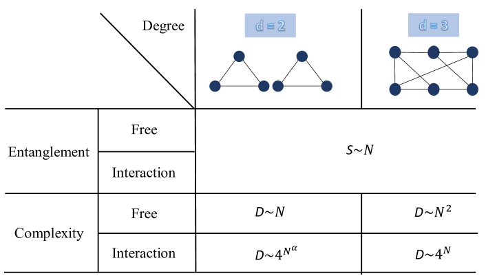
Figure 1: The scaling laws of entanglement and complexity for regular graph models with degrees $d=2$ and $d=3$. In all scenarios, entanglement adheres to volume laws, i.e., $S\sim N$. We unveil rich dynamical phases in these models by examining the Krylov complexity. For non-interacting fermions, the Krylov dimension $D$ with $d=2$ scales as $D\sim N$, whereas for $d=3$, it scales as $D\sim N^{2}$. In the interacting case, the scalings of the Krylov dimension for $d=2$, and $d=3$ are $D\sim 4^{N^{\alpha}}$ ($0.38\leq\alpha\leq 0.59$), and $D\sim 4^{N}$, respectively.

Entanglement typically serves as a distinguishing factor between different phases in dynamical phase transitions. In the context of many-body localization transitions, ergodic phases are characterized by linear growth of entanglement, whereas localization phases exhibit logarithmic growth [9]. Similar phenomena are observed in measurement-induced phase transitions, where linear growth denotes entangling phases and logarithmic growth denotes disentangling phases [12]. In our study, we observe the emergence of new phases characterized by Krylov complexity, as illustrated in Fig 1. Krylov complexity is proposed as a novel indicator for evaluating operator growth more directly and quantitatively [50]. It has received tremendous research efforts in various contexts such as quantum chaos and integrable systems [51, 52, 52, 53, 54], quantum field theory [55, 56, 57, 58], and open systems [59]. We investigate Krylov complexity for a half-filling free fermion model on regular graphs with $N$ sites. The results have been summarized in Fig  1. We note that quantum entanglement on different types of regular graphs with degrees $d=2$, and $d=3$ both obey volume law, with entanglement entropy $S$ scaling linearly in $\sim N$, yet their Krylov dimensions follow different scaling laws: $D$ scales as $\sim N$ for degree $d=2$ and $\sim N^{2}$ for $d=3$. To explicate the quantitative disparities between regular graphs of degrees $d=2$ and $d=3$, we develop a theory that captures the scaling laws precisely. Furthermore, we extend our analysis to incorporate interaction effects. In the interacting case, the Krylov dimension grows exponentially with system size. The exponential growth poses challenges for numerical methods in accurately determining the scaling law exponent. By extending our theory from the free case to the interacting case, we ascertain that the scaling laws become $D\sim 4^{N^{\alpha}}$. We find $0.38\leq\alpha\leq 0.59$ for $d=2$, whereas $\alpha=1$ for $d=3$. The distinctive dynamical phases characterized by different Krylov complexity scaling can be probed in atom tweezer experiments [42], by measuring the out-of-time-order correlations [60, 61].

Krylov complexity of free fermions on regular graphs.— To begin, we introduce a free fermion model on a graph, $G(E,V)$. The graph consists of a set of vertices $V$ and a set of edges $E$. Specifically, a regular graph $G_{R}$ is characterized by each vertex having an identical number of neighbors, indicating that every vertex shares the same degree. Within the framework of the free fermion model, each vertex of a regular graph corresponds to a site, while an edge denotes the tunneling between two such sites. Consequently, the Hamiltonian is represented as follows:

$$H_{\text{Free}}=\sum_{\{i,j\}\in E}J_{ij}a^{{\dagger}}_{i}a_{j},$$ (1)

where $i,j$ labels the vertices, $\{i,j\}\in E$ represent the edges in the graph. In this study, we focus on the case with $J_{ij}=J$. We consider $N$ sites at half-filling. The tunneling $J_{ij}$ is constrained to regular graphs of degree $d=2$ and $d=3$. Although we focus on the fermionic model, we expect the spin model also to exhibit analogous physics through the Jordan-Wigner transformation.

In the absence of interactions, fermionic many-body eigenstates are described as Slater-determinant product states. The entanglement entropy of these states is solely influenced by the two-point correlation function denoted as $C_{ij}=\braket{a^{{\dagger}}_{i}a_{j}}$ [62, 63]. By diagonalizing the correlation matrix within a local subsystem, we obtain eigenvalues $Z_{m}\in[0,1]$. Therefore, the Von Neumann entropy ($S$) for noninteracting eigenstates can be expressed as $S(l)=-\sum_{m=1}^{l}(1-Z_{m}){\rm ln}(1-Z_{m})+Z_{m}{\rm ln}Z_{m}$. Here, $l$ indicates the number of lattice sites within the subsystem. For our analysis, we set $l=N/2$, with the initial state occupying the first $N/2$ sites with $N/2$ fermions. We track the time evolution of the two-point correlation function, $C_{ij}(t)=\braket{a^{{\dagger}}_{i}(t)a_{j}(t)}$, where $a_{j}(t)=\exp{(-iH_{\text{Free}}t)}a_{j}\exp{(iH_{\text{Free}}t)}$, and evaluate the eigenvalue $Z_{m}(t)$. The Hamiltonian $H_{\text{Free}}$ is randomly selected from regular graphs with $d=2$ and $d=3$. The resulting findings are depicted in Fig. 2 (a), illustrating the average $S(N/2)$ over time and various sample graphs. By employing log-log plots and linear fitting, we establish scaling laws as $S\sim N^{1.06}$ for $d=2$ and $S\sim N^{1.00}$ for $d=3$. The entanglement for $d=2$ and $d=3$ both exhibit volume law scaling.

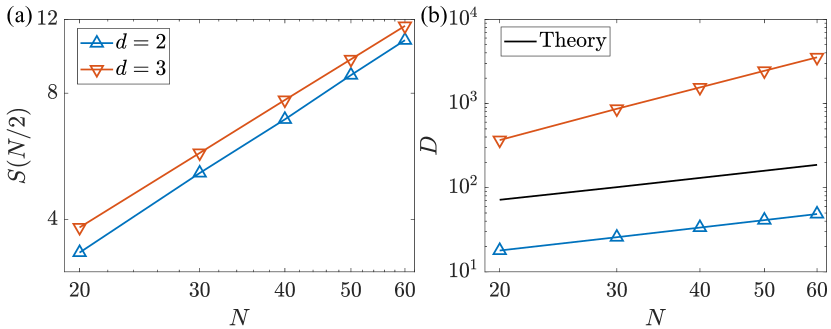
Figure 2: The entanglement and Krylov complexity of free fermions on regular graphs. (a), the scaling behavior of entanglement, $S(N/2)$, with respect to the system size $N$. We conduct simulations on $500$ random regular graphs with an evolution time of up to $10^{3}$ (in units of $\hbar/J$). We find entanglement volume law scaling for both $d=2$ and $d=3$ with $S\sim N$. (b), the scaling behavior of the Krylov dimension, $D$. For $d=2$, we average all non-isomorphic graphs. For $d=3$, we sample $500$ random non-isomorphic graphs. We find $D_{\text{Free}}^{d=2}\sim N^{0.91(4)}$ for $d=2$ and $D_{\text{Free}}^{d=3}\sim N^{2.03(3)}$ for $d=3$. The theoretical scaling laws approximate $D^{d=2}_{\text{Theory}}\sim N^{0.90}$ for $d=2$ and $D^{d=3}_{\text{Theory}}\sim N^{2.00}$ for $d=3$, which closely align with the numerical findings.

We proceed to examine the Krylov complexity in regular graphs and consider a many-body Hamiltonian $H$ and an initial local Hermitian operator $O$. The Heisenberg evolution of an operator is described by:

$$O(t)=e^{iHt}Oe^{-iHt}=\sum_{n=0}\frac{(it)^{n}}{n!}\mathcal{L}^{n}O$$ (2)

Here, $\mathcal{L}$ represents the Liouville operator, $\mathcal{L}|O)=|[H,O])$. The fictitious operator state is defined as $|O)=\sum_{ij}O_{ij}\ket{i}\bra{j}$, based on an orthonormal basis $\{\ket{i},\ket{j}\}$. The Krylov space is spanned by ${\mathcal{L}^{n}|O)}$, with its orthonormal basis introduced as ${|O_{n})}$ through the orthogonalization of ${\mathcal{L}^{n}|O)}$. The dimension $D$ of the Krylov space is determined by computing all the orthonormal Krylov bases (Supplementary Materials). This dimension $D$ characterizes the Krylov complexity of the quantum dynamics [50, 55, 64]. Additional results on Krylov complexity are provided in the supplementary material.

We delve into the Krylov dimension for regular graphs with degrees $d=2$ and $d=3$. In the subsequent analysis, we solely consider non-isomorphic regular graphs, as isomorphic ones exhibit identical Krylov complexities (Supplementary Materials). In our study, we investigate the operator growth [65, 50, 64] of particle number operators, $O_{i}=a^{{\dagger}}_{i}a_{i}$, where $i$ ranges from 1 to $N$. The corresponding results are illustrated in Fig. 2 (b). Our analysis involves studying the scaling laws associated with the Krylov dimension. Through log-log plots and linear fitting, we have established scaling relationships for the Krylov dimension. Specifically, for the Krylov dimension of free fermions on regular graphs of $d=2$ ($D_{\text{Free}}^{d=2}$), the scaling law is $D_{\text{Free}}^{d=2}\sim N^{0.91(4)}$. Similarly, for the Krylov dimension of free fermions on regular graphs of $d=3$ ($D_{\text{Free}}^{d=3}$), the scaling law is $D_{\text{Free}}^{d=3}\sim N^{2.03(3)}$. Although entanglement follows the scaling law of $S\sim N$ in both types of regular graphs, the scaling laws governing the Krylov dimension exhibit different trends between regular graphs with $d=2$ and $d=3$. This indicates that the dynamical phases on regular graphs are enriched by the scaling of the Krylov dimension. Dynamical phases that exhibit the same volume-law entanglement could display distinctive Krylov complexity, as demonstrated by our constructed free fermion model on regular graphs.

The distinctive behaviors in the Krylov complexity of regular graphs with $d=2$ and $d=3$ (Eq (1)) can be understood through their connectivity. As depicted in Fig. 1, regular graphs with $d=2$ consist of disconnected loops, while those with $d=3$ are almost fully interconnected. This structural contrast significantly impacts the Krylov complexity. Both the Hamiltonian $H_{\text{free}}$ and the local operator $O_{i}$ are quadratic operators, and their commutators are also quadratic operators. Consequently, the Krylov dimension scales approximately as $N^{2}$. This analysis is consistent with our findings for $d=3$. The free fermion Hamiltonian of regular graphs with $d=2$ ($H_{\text{Free}}^{d=2}$) can be represented as $H_{\text{Free}}^{d=2}=\sum_{l}H_{l}$, where $l$ represents distinct disconnected loops, each with a length of $n_{l}$, and $\sum_{l}n_{l}=N$. The operators $H_{l}$ mutually commute, i.e., $[H_{l},H_{l^{\prime}}]=0$. If our initial operator $O_{i}$ is positioned on a single loop $l$, the Krylov dimension is determined by the loop’s length $n_{l}$, not the system size $N$, due to the commuting property of $H_{l}$. Various initial operators $O_{i}$ may localize to different loops, each with its distinct length. This implies that the Krylov complexity of $d=2$ is much smaller than that of $d=3$. To evaluate the Krylov complexity of a regular graph with $d=2$, we need to average the selection of initial operators based on the probability $n_{l}/N$.

More quantitatively, we analyze the Krylov complexity of free fermions on regular graphs by averaging over their disconnected subgraphs. In our theoretical framework, we make a crucial assumption: the Krylov dimension of a free Hamiltonian defined on a graph is proportional to the square of the number of vertices connected to the vertex where the initial operator is located. This assumption is deemed reasonable, given that our focus is on extracting scaling laws rather than precisely determining the Krylov dimension. Furthermore, our findings indicate that the Krylov dimension for a free Hamiltonian defined on a loop scales proportionally to the square of the loop lengths (Supplementary Materials).

The theory consists of two primary components: one involves counting the number of non-isomorphic regular graphs with $d=2$, while the other entails evaluating the Krylov dimension for each non-isomorphic graph. Counting the number of non-isomorphic graphs is akin to solving the problem of partitioning $N$ into parts $\geq 3$, represented as $N=\sum_{l=1}^{M}n_{l},~{}3\leq n_{l}$, where $1\leq M\leq\lfloor\frac{N}{3}\rfloor$ denotes the number of integers. For instance, $M=2$ corresponds to partitioning $N$ vertices into two subsets. The independent ways of partition, denoted by $(n_{1},n_{2})$, are $[(3,N-3),(4,N-4),\cdots,(\lfloor N/2\rfloor,N-\lfloor N/2\rfloor)]$, with a total number of $C(N,M=2,I=3)=\lfloor\frac{N}{2}\rfloor-2$. Here, $I=3$ is the minimal integer in the decompositions, and the corresponding contribution to the Krylov dimension is denoted as $D_{\text{Free}}(N,M=2,I=3)$,

$$D_{\text{Free}}(N,M=2,I=3)=\sum_{3\leq k\leq\lfloor\frac{N}{2}\rfloor}k^{2}\frac{k}{N}+(N-k)^{2}\frac{N-k}{N},$$ (3)

where $\frac{k}{N}$ denotes the probability that the initial local operator is in the loop with a loop length of $k$. The factor $k^{2}$ and $(N-k)^{2}$ represent the corresponding the Krylov dimension. For any $M=m$, we derive a recurrence relationship as follows (Supplementary Materials):

$$C(N,m,I=3)=\sum_{3\leq k\leq\lfloor\frac{N-k}{m-1}\rfloor}C(N-k,m-1,k),$$ (4)

$$D_{\text{Free}}(N,m,I=3)=\sum_{3\leq k\leq\lfloor\frac{N-k}{m-1}\rfloor}k^{2}\frac{k}{N}+D(N,m-1,k).$$ (5)

Utilizing this recurrence, we can theoretically estimate the Krylov dimension of regular graphs with $d=2$, denoted as $D^{d=2}_{\text{Theory}}$, which is given by:

$$D^{d=2}_{\text{Theory}}=\frac{\sum_{M}D_{\text{Free}}(N,M,I=3)}{\sum_{M}C(N,M,I=3)}.$$ (6)

The corresponding results are illustrated in Fig. 2 (b). We observe that the scaling laws approximate $D^{d=2}_{\text{Theory}}\sim N^{0.90}$ for $d=2$, closely matching our numerical results. Conversely, for $d=3$, based on our assumption, we have $D^{d=3}_{\text{Theory}}\sim N^{2}$, as all non-isomorphic regular graphs with $d=3$ are nearly fully connected.

Interacting fermions on graphs.— We also investigate the interacting fermions model. The Hamiltonian is defined as follows:

$$H=\sum_{\{ij\}\in E}^{N}J_{ij}(a^{{\dagger}}_{i}a_{j}+n_{i}n_{j}),$$ (7)

where $n_{i}=a^{{\dagger}}_{i}a_{i}$ represents the particle number operator. Both the tunneling and interaction are defined using the same graphs, i.e., sharing the same factor $J_{ij}$. Based on the analysis of the free case, we discern that the disconnected properties of regular graphs with $d=2$ are crucial distinguishing features compared to the case of $d=3$. Tunneling and interaction determined by the same graph can preserve these properties.

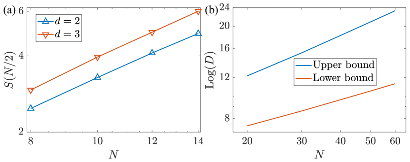
Figure 3: The entanglement and Krylov complexity for interacting fermions. (a), the scaling behavior of entanglement, $S(N/2)$, to the system size $N$. Simulations are conducted on $500$ random regular graphs with an evolution time of up to $10^{3}$ (in units of $\hbar/J$). We find that the entanglement of regular graphs with $d=2$ and $d=3$ scales with $S(N/2)\sim N$, adhering to the volume law. (b), the theoretical estimation of Krylov dimension. For regular graphs with $d=2$, the upper bound scales as $D^{d=2}_{\text{Int}}\sim 4^{N^{0.59}}$, while the lower bound scales as $D^{d=2}_{\text{Int}}\sim 4^{N^{0.38}}$.

The initial states are also half-filling. We track the time evolution of the initial state and evaluate the Von Neumann entropy $S(N/2)$. The Hamiltonian $H$ is randomly selected from regular graphs with $d=2$ and $d=3$. The resulting findings are depicted in Fig 3 (a), illustrating the average $S(N/2)$ over time across various sample graphs. We observe that both the entanglement of regular graphs with $d=2$ and $d=3$ scales with $S(N/2)\sim N$, satisfying the volume laws.

For interacting fermions, the computation cost for calculating the Krylov dimension grows exponentially with the system size. Our numerical simulations are restricted to relatively small systems (Supplementary Materials). We thus analyze the Krylov dimension of interacting fermions, by extending our analytic theory of the non-interacting case, instead of relying on small-size numerical calculations. A reasonable assumption to take is the Krylov dimension of an interacting Hamiltonian defined on a graph scales as $4^{L}$ (Supplementary Materials), where $L$ is the number of vertices connected to the vertex that the examined operator is initially located.

Based on this assumption, the Krylov dimension of interacting fermions on regular graphs with $d=3$ ($D^{d=3}_{\text{Int}}$) follows to the scaling law $D^{d=3}_{\text{Int}}\sim 4^{N}$, as almost all regular graphs with $d=3$ are connected. In the case of interacting fermions on regular graphs with $d=2$, we employ the same approach used in the free scenario. This involves the enumeration of non-isomorphic regular graphs and the subsequent evaluation of the Krylov dimension for each unique graph. In our interacting Hamiltonian setup, both tunneling and interaction are determined by the same graphs, implying that the count of non-isomorphic graphs remains unchanged between interaction and free cases, still denoted as $C(N,M,I)$. Regarding the Krylov dimension for each non-isomorphic graph in the interaction scenarios, we establish a recursive relationship. The corresponding Krylov dimension $D_{\text{int}}(N,m,I=3)$ is outlined as follows:

$$D_{\text{Int}}(N,m,I=3)=\sum_{3\leq k\leq\lfloor\frac{N-k}{m-1}\rfloor}4^{k}\frac{k}{N}+D(N,m-1,k),$$ (8)

where $4^{k}$ is the Krylov dimension that the initial local operator is in the loop with a loop length of $k$. The average Krylov dimension across non-isomorphic graphs computes as $D^{d=2}_{\text{Int}}=\sum_{M}D_{\text{Int}}(N,M,I=3)/\sum_{M}C(N,M,I=3)$. By calculating $D^{d=2}_{\text{Int}}$, we estimate the Krylov dimension, yielding a scaling law of $D^{d=2}_{\text{Int}}\sim 4^{N^{0.59}}$, as depicted in Fig 3 (b). This scaling law serves as an upper bound for the Krylov dimension, as $4^{L}$ is the maximum dimension of the operator space for an interacting fermion Hamiltonian defined on a loop of length $L$.

Here, we establish a lower bound by computing the average loop length $L^{d=2}$. We formulate a recursive relationship for the loop length $L$ (Supplementary Materials):

$$L(N,m,I=3)=\sum_{3\leq k\leq\lfloor\frac{N-k}{m-1}\rfloor}k\frac{k}{N}+L(N,m-1,k),$$ (9)

where $k$ represents the loop length housing the initial local operator. Through averaging across non-isomorphic graphs, the average loop length is determined as $L^{d=2}=\sum_{M}L(N,M,I=3)/\sum_{M}C(N,M,I=3)$. Based on our assumption, the Krylov dimension is $B\times 4^{L_{i}}$, where $B$ is a constant number and $L_{i}$ signifies the respective loop length. We infer that according to the arithmetic mean surpassing or equating the geometric mean, $B\times 4^{L^{d=2}}$ will be less than or equal to the average of $B\times 4^{L_{i}}$ across various non-isomorphic graphs. Consequently, by computing $4^{L^{d=2}}$, we arrive at a lower bound, leading to $D^{d=2}_{\text{Int}}\sim 4^{L^{d=2}}$. Upon evaluating $L^{d=2}$, we estimate the Krylov dimension, resulting in $D^{d=2}_{\text{Int}}\sim 4^{0.38}$, as illustrated in Fig 3 (b).

Out-of-time-order correlation.— To probe the distinctive dynamical phases on the graph enriched by the complexity, we propose to examine the quantum dynamics of atom tweezer arrays, where non-local couplings can be engineered by moving the atoms individually [48, 49]. It is worth noting that direct measurement of the Krylov complexity is practically infeasible. Nonetheless, the dynamical phases of regular graphs with $d=2$ and $d=3$ having distinctive complexity also produce qualitatively different OTOC behaviors (Supplementary Materials), which can then be measured in experiments [66, 67, 68, 69]. We thus expect the complexity enriched dynamical phases to be accessible to current experiments.

Conclusion and Outlook.— We have explored entanglement and Krylov complexity for fermions on regular graphs with degrees $d=2$ and $d=3$. The non-local tunnelings and interactions in the graph models may be realized by ⁶Li atoms confined by tweezers [70]. Entanglement scales as $S\sim N$ on both types of regular graphs with $d=2$ and $d=3$, whereas the Krylov complexity manifests distinct behaviors on these graphs. In the absence of interactions, the Krylov dimension scales as $D^{d=2}_{\text{Free}}\sim N^{0.91(4)}$ for $d=2$, and it scales as $D^{d=3}_{\text{Free}}\sim N^{2.03(3)}$ for $d=3$. With interactions, the Krylov dimension scales as $D^{d=2}_{\text{Int}}\sim 4^{N^{\alpha}}$ for $d=2$, where $0.38\leq\alpha\leq 0.59$, and $D^{d=3}_{\text{Int}}\sim 4^{N}$ for $d=3$. To interpret the rich behaviors of the Krylov complexity, we have developed an analytic theory that reproduces the intricate scaling of the Krylov dimension, having quantitative agreement with numerical simulations. The distinctions between the fermion dynamics on graphs with $d=2$ and $d=3$, with different complexity, can be probed through OTOC, which is accessible to current experiments. The potential phase transitions between the dynamical phases of different complexity are worth further investigation.

Acknowledgement.— This work is supported by National Key Research and Development Program of China (2021YFA1400900), National Natural Science Foundation of China (11934002), and Shanghai Municipal Science and Technology Major Project (Grant No. 2019SHZDZX01).

Appendix A Supplementary material

A.1 S1 The Krylov complexity

A.2 S1-1 The definition of Krylov complexity

We consider a Hamiltonian $H$ and an initial local Hermitian operator $O$. For any operator $O=\sum_{ij}O_{ij}\ket{i}\bra{j}$, defined on an orthonormal basis $\ket{i},\ket{j}$, the corresponding operator state is denoted as $|O)=\sum_{ij}O_{ij}\ket{i}\bra{j}$, and the inner product between two operator states is defined as:

$$(A|B)=\frac{Tr[A^{{\dagger}}B]}{Tr[\mathbf{I}]},$$ (S1)

where $\mathbf{I}$ is the identity matrix. The Heisenberg evolution of the operator $O$ is given by:

$$O(t)=e^{iHt}Oe^{-iHt}=\sum_{n=0}\frac{(it)^{n}}{n!}\mathcal{L}^{n}O,$$ (S2)

where $\mathcal{L}|O)=|[H,O])$. Equivalently, the Heisenberg evolution can be expressed as:

$$|O(t))=\sum_{n=0}\frac{(it)^{n}}{n!}\mathcal{L}^{n}|O).$$ (S3)

The Krylov space is spanned by ${\mathcal{L}^{n}|O\rangle}$. Typically, the Lanczos algorithm is utilized to generate an orthonormal basis of the Krylov space $\{|O_{n})\}$. Starting with the initial operator $|O_{0})=|O)$, we have $|O_{1})=b_{1}^{-1}\mathcal{L}|O_{0})$, where $b_{1}^{2}=(\mathcal{L}O_{0}|\mathcal{L}O_{0})$. For $n\geq 2$,

$$|A_{n}) = \mathcal{L}|O_{n-1})-b_{n-1}|O_{n-2}),$$ (S4)

$$b_{n}^{2} = (A_{n}|A_{n}),$$ (S5)

$$|O_{n}) = \frac{1}{b_{n}}|A_{n})$$ (S6)

It is known that the original Lanczos algorithm features a significant numerical instability: the construction of each Krylov element involves the two previous ones, causing errors due to finite-precision arithmetic to accumulate rapidly, leading to a loss of orthogonality in the Krylov basis during numerical computations. Residual overlaps between Krylov elements grow exponentially with the iteration number $n$, rendering the Lanczos coefficients unreliable after a few iterations. To address this issue, we adopt the following strategies [55]:

1. $|O_{0})=\frac{1}{\sqrt{(O|O)}}|O)$.

2. For $n\geq 1$: compute $|A_{n})=\mathcal{L}|O_{n-1})$.

3. Re-orthogonalize $|A_{n})$ explicitly with respect to all previous Krylov elements: $|A_{n})\rightarrow|A_{n})-\sum_{m=0}^{n-1}|O_{m})(O_{m}|A_{n})$.

4. Repeat step 3.

5. Set $b_{n}=\sqrt{(A_{n}|A_{n})}$.

6. if $b_{n}=0$ = stop; otherwise set $|O_{n})=\frac{1}{b_{n}}|A_{n})$ and go to step 2.

$|O_{n})$ involves an n-nested commutator with the Hamiltonian, and the operator becomes more complex and nonlocal with increasing orders of $n$. Therefore, the order $n$ can serve as a measure of operator complexity, motivating the definition of Krylov complexity:

$$C(t)=\sum_{n=0}^{D-1}n|(O(t)|O_{n})|^{2}.$$ (S7)

Here, $D$ represents the dimension of the Krylov space. In the Krylov basis, the Liouvillian operator’s matrix representation takes a tridiagonal form, with secondary diagonal elements $b_{n}$. By expanding the Heisenberg-evolved operator in the Krylov basis:

$$|O(t))=\sum_{n=0}^{K-1}\phi_{n}(t)|O_{n}),$$ (S8)

the Heisenberg equation of motion becomes:

$$-i\partial_{t}\phi_{n}(t)=b_{n}\phi_{n-1}(t)+b_{n+1}\phi_{n+1}(t).$$ (S9)

The initial condition is $\phi_{n}(0)=\delta_{n0}$, where $b_{0}=0$. Therefore, the equation of motion governing $b_{n}$ can be viewed as a single-particle hopping problem on a semi-infinite chain, with the hopping amplitudes $b_{n}$. We also have:

$$\vec{\phi}(t)=e^{-i\mathcal{L}t}\vec{\phi}(0),$$ (S10)

where $\vec{\phi}(t)=(\phi_{0}(t),\phi_{1}(t),\cdots)^{T}$. The Krylov complexity is the average position of the propagating packet over the Krylov chain:

$$C_{D}(t)=\sum_{n=0}^{D-1}n|\phi(t)|^{2}.$$ (S11)

A.3 S1-2 The numerical results of Krylov complexity

In the main text, we explored the scaling laws of the Krylov dimension with respect to the system size $N$. Here, in Fig 4, we illustrate the scaling laws of Krylov complexity. For regular graphs with $d=2$, the scaling laws are $C_{D}^{d=2}\sim N^{0.91(4)}$, and for $d=3$, $C_{D}^{d=3}\sim N^{2.03(3)}$. These results are consistent with the scaling laws of the Krylov dimension.

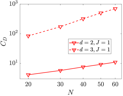
Figure 4: The scaling behavior of the Krylov complexity $C_{D}$ concerning the system size N. For regular graphs with $d=2$, we precisely evaluate the dimension by averaging across all non-isomorphic graphs. In the case of $d=3$, we sample 500 random non-isomorphic graphs. Through linear fitting, we determine scaling laws of $C_{D}^{d=2}\sim N^{0.91(4)}$ for $d=2$ and $C_{D}^{d=3}\sim N^{2.03(3)}$ for $d=3$.

We also explore the dimension of Krylov space and Krylov complexity in many-body scenarios. However, the exponentially large Krylov space, approximately $4^{N}$, renders numerical calculations impractical. Here, we present some results for small sizes, as depicted in Fig 5. We average over all non-isomorphic graphs and initial operators. It’s evident that both the Krylov space dimension $D$ and Krylov complexity $C_{D}$ increase exponentially. For regular graphs with $d=3$, the growth rate is faster than that for regular graphs with $d=2$. These numerical findings align with our theoretical estimations.

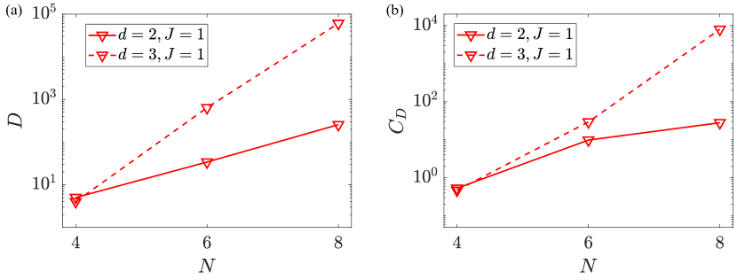
Figure 5: The numerical results of interacting fermions on graphs. (a) the plot of Krylov dimension $D$ as a function of system size $N$. (b) the plot of Krylov complexity $C_{D}$ with respect to system size $N$. For both regular graphs with $d=2$ and $d=3$, we average over all non-isomorphic graphs and initial operators. The time average extends up to $10^{3}$.

A.4 S2 The theoretical framework

We examine the free fermions Hamiltonian, $H_{\text{free}}=\sum_{ij}J_{ij}a^{\dagger}_{i}a_{j}$, and the local particle density operators $O_{i}=a^{\dagger}_{i}a_{i}$. Both $H_{\text{free}}$ and $O_{i}$ are quadratic operators, and their commutators are also quadratic operators. Thus, the Krylov space is spanned by quadratic operators, and the Krylov dimension scales as the square of the system size $N$, $D\sim N^{2}$. We also consider that for free fermions on regular graphs with $d=2$, the Hamiltonian can be rewritten as $H^{d=2}_{\text{free}}=\sum_{l}H_{l}$, where $l$ labels distinct disconnected loops, each with length $n_{l}$, and $\sum_{l}n_{l}=N$. The Hamiltonian $H_{l}$ defined on the disconnected subgraphs commutes with each other. The commutator $[\sum_{l}H_{l},O_{i}]=[H_{l_{i}},O_{i}]$, where $l_{i}$ represents the loop in which the vertex $i$ is located. Thus, the Krylov dimension is determined by the loop length $n_{l_{i}}$ rather than the system size $N$. Additionally, we focus on the scaling laws rather than the exact values of the dimension of the Krylov space. Based on the above observations, we make a reasonable assumption that the dimension of the Krylov space of a free Hamiltonian defined on a graph is proportional to the square of the number of vertices connected to the vertex where the initial operator is located. We also validate this assumption numerically. We create loops with varying lengths and examine their Krylov space dimension, as depicted in Fig 6. Through logarithmic plotting and linear fitting, we find that the dimension $D$ scales as $D\sim N^{2.00}$, consistent with our assumption.

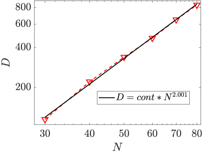
Figure 6: The dimension of Krylov space for loops with varying lengths.

Based on this assumption, considering that the non-isomorphic graphs of $d=3$ are almost connected, the scaling laws for regular graphs of $d=3$ are $D_{\text{Free}}^{d=3}\sim N^{2}$. Next, we derive the scaling laws for regular graphs of $d=2$. To achieve this, we need to count the number of non-isomorphic graphs, denoted as $C$, and determine Krylov dimension for each graph, denoted as $D$. The problem of determining the number of non-isomorphic graphs is equivalent to the problem of partitioning $N$ into parts $\geq 3$, such that $N=\sum_{l=1}^{M}n_{l}$, where $n_{l}\geq 3$, and $1\leq M\leq\lfloor\frac{N}{3}\rfloor$ represents the number of integers or the number of loops in regular graphs.

For $M=1$, there is only one decomposition, resulting in the number of decompositions $C(N,M=1,I=3)=1$, and the corresponding contribution to the Krylov space dimension is $D(N,M=1,I=3)=N^{2}$.

$$C(N,M=1,I=3)=1,$$ (S12)

$$D_{\text{Free}}(N,M=1,I=3)=N^{2}$$ (S13)

Here, $I$ is the minimum integer in the decompositions. For $M=2$, where $N=n_{1}+n_{2}$, there are $\lfloor\frac{N}{2}\rfloor-2$ decompositions, represented by $[(3,N-3),(4,N-4),\cdots,(\lfloor N/2\rfloor,N-\lfloor N/2\rfloor)]$. The corresponding contribution to the Krylov dimension is denoted as:

$$C(N,M=2,I=3) = \lfloor\frac{N}{2}\rfloor-2,$$ (S14)

$$D_{\text{Free}}(N,M=2,I=3) = \sum_{3\leq k\leq\lfloor\frac{N}{2}\rfloor}k^{2}\frac{k}{N}+(N-k)^{2}\frac{N-k}{N}.$$ (S15)

Here, $k$ represents the length of a loop, and $k^{2}$ is the corresponding dimension of the Krylov space. $\frac{k}{N}$ is the probability that the initial operator $O_{i}$ is located in this loop.

For $M=3$, our strategy involves dividing $N$ into two integers, $n_{1}$ and $n_{2}$, just as we do in $M=2$, and then further dividing $n_{2}$ into 2 integers. For example, $N=15$ can be divided into $n_{1}=3,n_{2}=12$ or $n_{1}=4,n_{2}=11$, then $n_{2}=3+9$ or $n_{2}=4+7$. However, there is repetitive counting, such as $n_{2}=4+8$ and $n_{2}=3+8$. The key point is to avoid this issue. We take $N=15$ as an example to elaborate on our method. The following table shows all the decompositions of $N=15$.

3	3	9
3	4	8
3	5	7
3	6	6
4	4	7
4	5	6
5	5	5

First, we set $n_{1}=3$, and $N-n_{1}$ is divided into 2 integers $[(3,9),(4,8),(5,7),(6,6)]$. Next, for $n_{1}=4$, to avoid repetition, the minimal integers of the decompositions $I$ should satisfy $I=4$. Similarly, for $n_{1}=5$, $I=5$. Thus,

$$C(N,M=3,I=3) = \sum_{3\leq k\leq\lfloor\frac{N-k}{2}\rfloor}C(N-k,M=2,k)$$ (S16)

$$D_{\text{Free}}(N,M=3,I=3) = \sum_{3\leq k\leq\lfloor\frac{N-k}{2}\rfloor}k^{2}\frac{k}{N}+D_{\text{Free}}(N,M=2,k).$$ (S17)

Similarly, we derive the recurrence for any $M$:

$$C(N,M,I=3) = \sum_{3\leq k\leq\lfloor\frac{N-k}{M-1}\rfloor}C(N-k,M-1,k)$$ (S18)

$$D_{\text{Free}}(N,M,I=3) = \sum_{3\leq k\leq\lfloor\frac{N-k}{M-1}\rfloor}k^{2}\frac{k}{N}+D_{\text{Free}}(N,M-1,k).$$ (S19)

Based on the recurrence relation, the dimension of Krylov space $D^{d=2}=\sum_{M}D_{\text{Free}}(N,M,I=3)/\sum_{M}C(N,M,I=3)$.

The theory can also be extended to include interacting fermions on graphs. In this scenario, the Krylov space is not solely spanned by quadratic operators but also encompasses other many-body operators. Consequently, we have revised the assumption made in the free case, now positing that the Krylov dimension of an interacting Hamiltonian defined on a graph is proportional to $4^{L}$, where $L$ denotes the number of vertices connected to the vertex where the initial operator is located. Similarly, we can derive a recurrence relation for the interacting case:

$$D_{\text{Int}}(N,M,I=3)=\sum_{3\leq k\leq\lfloor\frac{N-k}{M-1}\rfloor}4^{k}\frac{k}{N}+D_{\text{Int}}((N,M-1,k).$$ (S20)

The Krylov dimension of interacting fermions $D_{\text{Int}}^{d=2}=\sum_{M}D_{\text{Int}}(N,M,I=3)/\sum_{M}C(N,M,I=3)$.

This method can also be utilized to calculate the loop length. In the case of regular graphs with $d=3$, where the graphs are almost entirely connected, the loop length equals $N$. However, for regular graphs with $d=2$, the loop length of a non-isomorphic graph is determined by:

$$L(N,M,I=3)=\sum_{3\leq k\leq\lfloor\frac{N-k}{M-1}\rfloor}k\frac{k}{N}+L((N,M-1,k).$$ (S21)

$K$ is the length of a loop. The average loop length of interacting fermions in the case of $d=2$ is $L^{d=2}=\sum_{M}L(N,M,I=3)/\sum_{M}D(N,M,I=3)$ and the scaling laws of Krylov dimension is $\sim 4^{L^{d=2}}$

A.5 S3 The out-of-time-order correlation

The OTOC is a time-dependent function defined by an averaged double-commutator as

$$C(t)=\braket{[O(t),Q]^{{\dagger}}[O(t),Q]}.$$ (S22)

If $O$ and $Q$ are both hermitian and unitary,

$$C(t)=2(1-Re(F(t))),$$ (S23)

where $F(t)=\braket{O(t)^{{\dagger}}Q^{{\dagger}}O(t)Q}$. The OTOC can be detected in experiments and used to distinguish between regular graphs with degrees 2 and 3. The most significant disparity between degrees 2 and 3 is evident in the structure of the regular graphs. A degree-2 regular graph consists of disconnected loops, while a degree-3 regular graph is nearly connected. This contrast can be discerned using the OTOC. In a degree-2 regular graph, the operators $O(t)$ and $Q$ commute if their support belongs to different loops, resulting in $C(t)=0$. However, this scenario is rare in the case of degree 3.

Here, we consider the operators $O=2a_{1}^{{\dagger}}a_{1}-\mathbf{I}$ and $Q=2a_{N/2}^{{\dagger}}a_{N/2}-\mathbf{I}$ to ensure that $Q$ and $O$ are unitary and Hermitian. We investigate the quantity $F(t)$ averaged over non-isomorphic graphs, as depicted in Fig 7. Fig 7 (a) shows the results for free fermions with $N=20$, while Fig 7 (b) displays the results for interacting fermions with $N=14$. For regular graphs of $d=2$, $F(t)$ remains close to 1 in both the free and interacting cases, indicating that the system does not undergo scrambling. However, in the case of $d=3$, $F(t)$ decreases and stabilizes, suggesting that the system undergoes scrambling. This notable difference in experimental observations highlights distinct dynamical phases in regular graphs of $d=2$ and $d=3$.

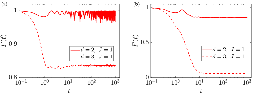
Figure 7: The numerical results of OTOC. (a), the plot of $F(t)$ as a function of $t$ for free fermions. (b), the plot of $F(t)$ as a function of $t$ for interacting fermions. The initial operators considered are $O=2a_{1}^{{\dagger}}a_{1}-\mathbf{I}$ and $Q=2a_{N/2}^{{\dagger}}a_{N/2}-\mathbf{I}$. In the free case, the system size is $N=20$. We sample all non-isomorphic graphs for regular graphs of $d=2$ and 500 non-isomorphic graphs for regular graphs of $d=3$. In the interacting case, the system size is $N=14$, and we sample all non-isomorphic regular graphs for both $d=2$ and $d=3$.

A.6 S4 The discussion about the non-isomorphic graphs

In the main text, we focus exclusively on non-isomorphic graphs. Let’s explore this concept further. We begin with the free Hamiltonian $H_{\text{free}}=\sum_{\{i,j\}\in E}J_{ij}a^{{\dagger}}_{i}a_{j}$, defined over the operator basis ${a^{{\dagger}}_{i},a_{j}}$. Here, $J$ denotes our Hamiltonian. In the case of isomorphic regular graphs, typically, there exists a permutation difference between them. Consequently, the original commutator $[H,O_{i}]$ is transformed into $[PHP^{{\dagger}},O_{i}]$, where $P$ represents a permutation transformation. Since $[PHP^{{\dagger}},O_{i}]=P[H,P^{{\dagger}}O_{i}P]P^{{\dagger}}$ and $P^{{\dagger}}O_{i}P\neq O_{i}$, the dimension of the Krylov space for isomorphic graphs may vary. However, it’s important to note that the initial operator $O_{i}$ is diagonal, and $O_{j}=P^{{\dagger}}O_{i}P$ is also diagonal. Therefore, when summing over all initial operators, $\sum_{i}O_{i}=\sum_{i}P^{{\dagger}}O_{i}P$, since $\sum_{i}O_{i}=\mathbf{I}$. This implies that the dimension of the Krylov space for isomorphic graphs is the same based on the average of the initial operators.

For interacting fermions on regular graphs, represented by the Hamiltonian $H=\sum_{\{ij\}\in E}^{N}J_{ij}(a^{{\dagger}}_{i}a_{j}+n_{i}n_{j})$, isomorphic graphs are related by $J\rightarrow J^{\prime}=PJP^{{\dagger}}$. Here, $J$ and $J^{\prime}$ correspond to two Hamiltonians $H$ and $H^{\prime}$ in the many-body basis, respectively. We observe that the two Hamiltonians differ only by relabelling the indices ${i,j}\rightarrow{i^{\prime},j^{\prime}}$. Hence, similarly, the dimension of the Krylov space for isomorphic graphs remains the same, based on the average of the initial operators.

To validate the aforementioned arguments, we conducted a numerical investigation of the dimension of the Krylov space for isomorphic graphs. We selected a regular graph $G_{R}$ and generated an isomorphic graph $G^{\prime}_{R}$ by applying a random permutation to the adjacency matrix. The dimension of the Krylov space for both $G_{R}$ and $G^{\prime}_{R}$, denoted as $D(G_{R})$ and $D(G^{\prime}_{R})$ respectively, was computed. We then averaged the results over all initial operators $O_{i},~{}i\in[1,N]$. The corresponding outcomes are depicted in Fig 8. In our analysis, we sampled 40 non-isomorphic regular graphs, with the x-coordinate $G$ representing different non-isomorphic graphs. We defined the ratio $R=D(G_{R})/D(G^{\prime}_{R})$ to quantify the difference between the two isomorphic graphs. From the numerical results, it was evident that the ratio $R$ equaled exactly 1. This implies that isomorphic graphs exhibit the same dimension of Krylov space, validating our theoretical analysis. Similar conclusions were reached for interacting fermions. However, it’s worth noting that due to computational constraints, we were only able to investigate very small system sizes in many-body cases, and the number of non-isomorphic graphs was limited. For instance, When $N=12,$the number of non-isomorphic regular graphs of $d=2$ was only 2. Therefore, we did not present the numerical results for interacting fermions.

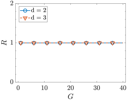
Figure 8: The dimension of the Krylov space for isomorphic regular graphs. The x-coordinate $G$ represents different non-isomorphic regular graphs. We sampled 40 non-isomorphic regular graphs, as this encompasses the total number of non-isomorphic regular graphs of $d=2$, which is approximately 40. The results are averaged over all initial operators.

A.7 S5 The effect of disorder

We also explore the effects of disorder on free fermions in graphs. The Hamiltonian is defined as follows:

$$H_{\text{dis}}=\sum_{\{i,j\}\in E}J_{ij}a^{{\dagger}}_{i}a_{j}+\sum_{i\in G_{R}}W_{i}a^{{\dagger}}_{i}a_{i}.$$ (S24)

Here, we introduce on-site disorder to the Hamiltonian, with $W_{i}$ representing the disorder strength, uniformly distributed in the range $[-W,W]$. We examine the Krylov complexity, as illustrated in Fig  9. In this analysis, we sample 200 disorder instances with $N=50$. An intriguing observation emerges: for regular graphs of $d=3$, the Krylov complexity decreases with increasing disorder strength. This outcome is expected, as disorder typically induces localization. However, for $d=2$, the Krylov complexity initially increases and then decreases with disorder. We speculate that this behavior arises from the interplay between symmetry and disorder.

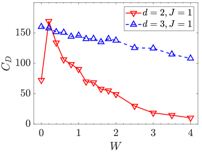
Figure 9: The Krylov complexity of disorder-free fermions on graphs. We consider a system size of $N=50$ and sample 200 disorder configurations.

References

- Heyl [2018] M. Heyl, Dynamical quantum phase transitions: a review, Reports on Progress in Physics 81, 054001 (2018).
- Zvyagin [2016] A. A. Zvyagin, Dynamical quantum phase transitions (Review Article), Low Temperature Physics 42, 971 (2016), https://pubs.aip.org/aip/ltp/article-pdf/42/11/971/16095119/971_1_online.pdf .
- Heyl et al. [2013] M. Heyl, A. Polkovnikov, and S. Kehrein, Dynamical quantum phase transitions in the transverse-field ising model, Phys. Rev. Lett. 110, 135704 (2013).
- Heyl [2014] M. Heyl, Dynamical quantum phase transitions in systems with broken-symmetry phases, Phys. Rev. Lett. 113, 205701 (2014).
- Vosk and Altman [2014] R. Vosk and E. Altman, Dynamical quantum phase transitions in random spin chains, Phys. Rev. Lett. 112, 217204 (2014).
- Heyl [2015a] M. Heyl, Scaling and universality at dynamical quantum phase transitions, Phys. Rev. Lett. 115, 140602 (2015a).
- Jurcevic et al. [2017a] P. Jurcevic, H. Shen, P. Hauke, C. Maier, T. Brydges, C. Hempel, B. P. Lanyon, M. Heyl, R. Blatt, and C. F. Roos, Direct observation of dynamical quantum phase transitions in an interacting many-body system, Phys. Rev. Lett. 119, 080501 (2017a).
- Nandkishore and Huse [2015] R. Nandkishore and D. A. Huse, Many-body localization and thermalization in quantum statistical mechanics, Annual Review of Condensed Matter Physics 6, 15 (2015), https://doi.org/10.1146/annurev-conmatphys-031214-014726 .
- Abanin et al. [2019] D. A. Abanin, E. Altman, I. Bloch, and M. Serbyn, Colloquium: Many-body localization, thermalization, and entanglement, Rev. Mod. Phys. 91, 021001 (2019).
- Pal and Huse [2010] A. Pal and D. A. Huse, Many-body localization phase transition, Phys. Rev. B 82, 174411 (2010).
- Alet and Laflorencie [2018] F. Alet and N. Laflorencie, Many-body localization: An introduction and selected topics, Comptes Rendus Physique 19, 498 (2018).
- Skinner et al. [2019] B. Skinner, J. Ruhman, and A. Nahum, Measurement-induced phase transitions in the dynamics of entanglement, Phys. Rev. X 9, 031009 (2019).
- Koh et al. [2023] J. M. Koh, S.-N. Sun, M. Motta, and A. J. Minnich, Measurement-induced entanglement phase transition on a superconducting quantum processor with mid-circuit readout, Nature Physics 19, 1314 (2023).
- Choi et al. [2020] S. Choi, Y. Bao, X.-L. Qi, and E. Altman, Quantum error correction in scrambling dynamics and measurement-induced phase transition, Phys. Rev. Lett. 125, 030505 (2020).
- Gullans and Huse [2020] M. J. Gullans and D. A. Huse, Dynamical purification phase transition induced by quantum measurements, Phys. Rev. X 10, 041020 (2020).
- Vajna and Dóra [2015] S. Vajna and B. Dóra, Topological classification of dynamical phase transitions, Phys. Rev. B 91, 155127 (2015).
- Huang and Balatsky [2016] Z. Huang and A. V. Balatsky, Dynamical quantum phase transitions: Role of topological nodes in wave function overlaps, Phys. Rev. Lett. 117, 086802 (2016).
- Budich and Heyl [2016] J. C. Budich and M. Heyl, Dynamical topological order parameters far from equilibrium, Phys. Rev. B 93, 085416 (2016).
- Bhattacharya and Dutta [2017] U. Bhattacharya and A. Dutta, Emergent topology and dynamical quantum phase transitions in two-dimensional closed quantum systems, Phys. Rev. B 96, 014302 (2017).
- Fläschner et al. [2018] N. Fläschner, D. Vogel, M. Tarnowski, B. Rem, D.-S. Lühmann, M. Heyl, J. Budich, L. Mathey, K. Sengstock, and C. Weitenberg, Observation of dynamical vortices after quenches in a system with topology, Nature Physics 14, 265 (2018).
- Sharma et al. [2016] S. Sharma, U. Divakaran, A. Polkovnikov, and A. Dutta, Slow quenches in a quantum ising chain: Dynamical phase transitions and topology, Phys. Rev. B 93, 144306 (2016).
- Bhattacharya et al. [2017] U. Bhattacharya, S. Bandyopadhyay, and A. Dutta, Mixed state dynamical quantum phase transitions, Phys. Rev. B 96, 180303 (2017).
- Heyl [2015b] M. Heyl, Scaling and universality at dynamical quantum phase transitions, Phys. Rev. Lett. 115, 140602 (2015b).
- Karrasch and Schuricht [2017] C. Karrasch and D. Schuricht, Dynamical quantum phase transitions in the quantum potts chain, Phys. Rev. B 95, 075143 (2017).
- Jurcevic et al. [2017b] P. Jurcevic, H. Shen, P. Hauke, C. Maier, T. Brydges, C. Hempel, B. P. Lanyon, M. Heyl, R. Blatt, and C. F. Roos, Direct observation of dynamical quantum phase transitions in an interacting many-body system, Phys. Rev. Lett. 119, 080501 (2017b).
- yoon Choi et al. [2016] J. yoon Choi, S. Hild, J. Zeiher, P. Schauß, A. Rubio-Abadal, T. Yefsah, V. Khemani, D. A. Huse, I. Bloch, and C. Gross, Exploring the many-body localization transition in two dimensions, Science 352, 1547 (2016), https://www.science.org/doi/pdf/10.1126/science.aaf8834 .
- Muniz et al. [2020] J. A. Muniz, D. Barberena, R. J. Lewis-Swan, D. J. Young, J. R. Cline, A. M. Rey, and J. K. Thompson, Exploring dynamical phase transitions with cold atoms in an optical cavity, Nature 580, 602 (2020).
- Smale et al. [2019] S. Smale, P. He, B. A. Olsen, K. G. Jackson, H. Sharum, S. Trotzky, J. Marino, A. M. Rey, and J. H. Thywissen, Observation of a transition between dynamical phases in a quantum degenerate fermi gas, Science Advances 5, eaax1568 (2019), https://www.science.org/doi/pdf/10.1126/sciadv.aax1568 .
- Tian et al. [2020] T. Tian, H.-X. Yang, L.-Y. Qiu, H.-Y. Liang, Y.-B. Yang, Y. Xu, and L.-M. Duan, Observation of dynamical quantum phase transitions with correspondence in an excited state phase diagram, Phys. Rev. Lett. 124, 043001 (2020).
- goo [2023] Measurement-induced entanglement and teleportation on a noisy quantum processor, Nature 622, 481 (2023).
- Dborin et al. [2022] J. Dborin, V. Wimalaweera, F. Barratt, E. Ostby, T. E. O’Brien, and A. G. Green, Simulating groundstate and dynamical quantum phase transitions on a superconducting quantum computer, Nature Communications 13, 5977 (2022).
- Xu et al. [2020] K. Xu, Z.-H. Sun, W. Liu, Y.-R. Zhang, H. Li, H. Dong, W. Ren, P. Zhang, F. Nori, D. Zheng, H. Fan, and H. Wang, Probing dynamical phase transitions with a superconducting quantum simulator, Science Advances 6, eaba4935 (2020), https://www.science.org/doi/pdf/10.1126/sciadv.aba4935 .
- Bluvstein et al. [2021] D. Bluvstein, A. Omran, H. Levine, A. Keesling, G. Semeghini, S. Ebadi, T. T. Wang, A. A. Michailidis, N. Maskara, W. W. Ho, S. Choi, M. Serbyn, M. Greiner, V. Vuletić, and M. D. Lukin, Controlling quantum many-body dynamics in driven rydberg atom arrays, Science 371, 1355 (2021), https://www.science.org/doi/pdf/10.1126/science.abg2530 .
- Ding et al. [2024] D. Ding, Z. Bai, Z. Liu, B. Shi, G. Guo, W. Li, and C. S. Adams, Ergodicity breaking from rydberg clusters in a driven-dissipative many-body system, Science Advances 10, eadl5893 (2024), https://www.science.org/doi/pdf/10.1126/sciadv.adl5893 .
- Wu et al. [2023] X. Wu, Z. Wang, F. Yang, R. Gao, C. Liang, M. K. Tey, X. Li, T. Pohl, and L. You, Observation of a dissipative time crystal in a strongly interacting rydberg gas (2023), arXiv:2305.20070 [cond-mat.quant-gas] .
- Liu et al. [2024] B. Liu, L.-H. Zhang, Z.-K. Liu, J. Zhang, Z.-Y. Zhang, S.-Y. Shao, Q. Li, H.-C. Chen, Y. Ma, T.-Y. Han, Q.-F. Wang, D.-S. Ding, and B.-S. Shi, Bifurcation of time crystals in driven and dissipative rydberg atomic gas (2024), arXiv:2402.13644 [cond-mat.quant-gas] .
- Omran et al. [2019] A. Omran, H. Levine, A. Keesling, G. Semeghini, T. T. Wang, S. Ebadi, H. Bernien, A. S. Zibrov, H. Pichler, S. Choi, J. Cui, M. Rossignolo, P. Rembold, S. Montangero, T. Calarco, M. Endres, M. Greiner, V. Vuletić, and M. D. Lukin, Generation and manipulation of schrödinger cat states in rydberg atom arrays, Science 365, 570 (2019), https://www.science.org/doi/pdf/10.1126/science.aax9743 .
- Scholl et al. [2021] P. Scholl, M. Schuler, H. J. Williams, A. A. Eberharter, D. Barredo, K.-N. Schymik, V. Lienhard, L.-P. Henry, T. C. Lang, T. Lahaye, et al., Quantum simulation of 2d antiferromagnets with hundreds of rydberg atoms, Nature 595, 233 (2021).
- Bluvstein et al. [2022] D. Bluvstein, H. Levine, G. Semeghini, T. T. Wang, S. Ebadi, M. Kalinowski, A. Keesling, N. Maskara, H. Pichler, M. Greiner, et al., A quantum processor based on coherent transport of entangled atom arrays, Nature 604, 451 (2022).
- Bornet et al. [2023] G. Bornet, G. Emperauger, C. Chen, B. Ye, M. Block, M. Bintz, J. A. Boyd, D. Barredo, T. Comparin, F. Mezzacapo, et al., Scalable spin squeezing in a dipolar rydberg atom array, Nature 621, 728 (2023).
- Browaeys and Lahaye [2020] A. Browaeys and T. Lahaye, Many-body physics with individually controlled rydberg atoms, Nature Physics 16, 132 (2020).
- Ebadi et al. [2022] S. Ebadi, A. Keesling, M. Cain, T. T. Wang, H. Levine, D. Bluvstein, G. Semeghini, A. Omran, J.-G. Liu, R. Samajdar, X.-Z. Luo, B. Nash, X. Gao, B. Barak, E. Farhi, S. Sachdev, N. Gemelke, L. Zhou, S. Choi, H. Pichler, S.-T. Wang, M. Greiner, V. Vuletić, and M. D. Lukin, Quantum optimization of maximum independent set using rydberg atom arrays, Science 376, 1209 (2022), https://www.science.org/doi/pdf/10.1126/science.abo6587 .
- Kim et al. [2022] M. Kim, K. Kim, J. Hwang, E.-G. Moon, and J. Ahn, Rydberg quantum wires for maximum independent set problems, Nature Physics 18, 755 (2022).
- Goswami et al. [2023] K. Goswami, R. Mukherjee, H. Ott, and P. Schmelcher, Solving optimization problems with local light shift encoding on rydberg quantum annealers (2023), arXiv:2308.07798 [quant-ph] .
- Zhou et al. [2020] L. Zhou, S.-T. Wang, S. Choi, H. Pichler, and M. D. Lukin, Quantum approximate optimization algorithm: Performance, mechanism, and implementation on near-term devices, Phys. Rev. X 10, 021067 (2020).
- Nguyen et al. [2023] M.-T. Nguyen, J.-G. Liu, J. Wurtz, M. D. Lukin, S.-T. Wang, and H. Pichler, Quantum optimization with arbitrary connectivity using rydberg atom arrays, PRX Quantum 4, 010316 (2023).
- Wild et al. [2021] D. S. Wild, D. Sels, H. Pichler, C. Zanoci, and M. D. Lukin, Quantum sampling algorithms for near-term devices, Phys. Rev. Lett. 127, 100504 (2021).
- Barredo et al. [2016] D. Barredo, S. De Léséleuc, V. Lienhard, T. Lahaye, and A. Browaeys, An atom-by-atom assembler of defect-free arbitrary two-dimensional atomic arrays, Science 354, 1021 (2016).
- Endres et al. [2016] M. Endres, H. Bernien, A. Keesling, H. Levine, E. R. Anschuetz, A. Krajenbrink, C. Senko, V. Vuletic, M. Greiner, and M. D. Lukin, Atom-by-atom assembly of defect-free one-dimensional cold atom arrays, Science 354, 1024 (2016).
- Parker et al. [2019] D. E. Parker, X. Cao, A. Avdoshkin, T. Scaffidi, and E. Altman, A universal operator growth hypothesis, Phys. Rev. X 9, 041017 (2019).
- Rabinovici et al. [2021] E. Rabinovici, A. Sánchez-Garrido, R. Shir, and J. Sonner, Operator complexity: a journey to the edge of krylov space, Journal of High Energy Physics 2021, 1 (2021).
- Rabinovici et al. [2022] E. Rabinovici, A. Sánchez-Garrido, R. Shir, and J. Sonner, Krylov complexity from integrability to chaos, Journal of High Energy Physics 2022, 1 (2022).
- Hashimoto et al. [2023] K. Hashimoto, K. Murata, N. Tanahashi, and R. Watanabe, Krylov complexity and chaos in quantum mechanics, Journal of High Energy Physics 2023, 1 (2023).
- Trigueros and Lin [2022] F. B. Trigueros and C.-J. Lin, Krylov complexity of many-body localization: Operator localization in Krylov basis, SciPost Phys. 13, 037 (2022).
- Barbón et al. [2019] J. Barbón, E. Rabinovici, R. Shir, and R. Sinha, On the evolution of operator complexity beyond scrambling, Journal of High Energy Physics 2019, 1 (2019).
- Dymarsky and Smolkin [2021] A. Dymarsky and M. Smolkin, Krylov complexity in conformal field theory, Phys. Rev. D 104, L081702 (2021).
- Avdoshkin et al. [2022] A. Avdoshkin, A. Dymarsky, and M. Smolkin, Krylov complexity in quantum field theory, and beyond (2022), arXiv:2212.14429 [hep-th] .
- Kundu et al. [2023] A. Kundu, V. Malvimat, and R. Sinha, State dependence of krylov complexity in 2d cfts, Journal of High Energy Physics 2023, 1 (2023).
- Liu et al. [2023] C. Liu, H. Tang, and H. Zhai, Krylov complexity in open quantum systems, Phys. Rev. Res. 5, 033085 (2023).
- Hashimoto et al. [2017] K. Hashimoto, K. Murata, and R. Yoshii, Out-of-time-order correlators in quantum mechanics, Journal of High Energy Physics 2017, 1 (2017).
- Swingle [2018] B. Swingle, Unscrambling the physics of out-of-time-order correlators, Nature Physics 14, 988 (2018).
- Peschel [2003] I. Peschel, Calculation of reduced density matrices from correlation functions, Journal of Physics A: Mathematical and General 36, L205 (2003).
- Li et al. [2016] X. Li, J. H. Pixley, D.-L. Deng, S. Ganeshan, and S. Das Sarma, Quantum nonergodicity and fermion localization in a system with a single-particle mobility edge, Phys. Rev. B 93, 184204 (2016).
- Caputa et al. [2024] P. Caputa, H.-S. Jeong, S. Liu, J. F. Pedraza, and L.-C. Qu, Krylov complexity of density matrix operators (2024), arXiv:2402.09522 [hep-th] .
- Bhattacharyya et al. [2023] A. Bhattacharyya, D. Ghosh, and P. Nandi, Operator growth and krylov complexity in bose-hubbard model, Journal of High Energy Physics 2023, 1 (2023).
- Li et al. [2017] J. Li, R. Fan, H. Wang, B. Ye, B. Zeng, H. Zhai, X. Peng, and J. Du, Measuring out-of-time-order correlators on a nuclear magnetic resonance quantum simulator, Phys. Rev. X 7, 031011 (2017).
- Mi et al. [2021] X. Mi, P. Roushan, C. Quintana, S. Mandrà, J. Marshall, C. Neill, F. Arute, K. Arya, J. Atalaya, R. Babbush, J. C. Bardin, R. Barends, J. Basso, A. Bengtsson, S. Boixo, A. Bourassa, M. Broughton, B. B. Buckley, D. A. Buell, B. Burkett, N. Bushnell, Z. Chen, B. Chiaro, R. Collins, W. Courtney, S. Demura, A. R. Derk, A. Dunsworth, D. Eppens, C. Erickson, E. Farhi, A. G. Fowler, B. Foxen, C. Gidney, M. Giustina, J. A. Gross, M. P. Harrigan, S. D. Harrington, J. Hilton, A. Ho, S. Hong, T. Huang, W. J. Huggins, L. B. Ioffe, S. V. Isakov, E. Jeffrey, Z. Jiang, C. Jones, D. Kafri, J. Kelly, S. Kim, A. Kitaev, P. V. Klimov, A. N. Korotkov, F. Kostritsa, D. Landhuis, P. Laptev, E. Lucero, O. Martin, J. R. McClean, T. McCourt, M. McEwen, A. Megrant, K. C. Miao, M. Mohseni, S. Montazeri, W. Mruczkiewicz, J. Mutus, O. Naaman, M. Neeley, M. Newman, M. Y. Niu, T. E. O’Brien, A. Opremcak, E. Ostby, B. Pato, A. Petukhov, N. Redd, N. C. Rubin, D. Sank, K. J. Satzinger, V. Shvarts, D. Strain, M. Szalay, M. D. Trevithick, B. Villalonga, T. White, Z. J. Yao, P. Yeh, A. Zalcman, H. Neven, I. Aleiner, K. Kechedzhi, V. Smelyanskiy, and Y. Chen, Information scrambling in quantum circuits, Science 374, 1479 (2021), https://www.science.org/doi/pdf/10.1126/science.abg5029 .
- Green et al. [2022] A. M. Green, A. Elben, C. H. Alderete, L. K. Joshi, N. H. Nguyen, T. V. Zache, Y. Zhu, B. Sundar, and N. M. Linke, Experimental measurement of out-of-time-ordered correlators at finite temperature, Phys. Rev. Lett. 128, 140601 (2022).
- Landsman et al. [2019] K. A. Landsman, C. Figgatt, T. Schuster, N. M. Linke, B. Yoshida, N. Y. Yao, and C. Monroe, Verified quantum information scrambling, Nature 567, 61 (2019).
- Yan et al. [2022] Z. Z. Yan, B. M. Spar, M. L. Prichard, S. Chi, H.-T. Wei, E. Ibarra-García-Padilla, K. R. A. Hazzard, and W. S. Bakr, Two-dimensional programmable tweezer arrays of fermions, Phys. Rev. Lett. 129, 123201 (2022).