Testing common approximations to predict the 21cm signal at the Epoch of Reionization and Cosmic dawn
Abstract
Predicting the 21cm signal from the epoch of reionization and cosmic dawn is a complex and challenging task. Various simplifying assumptions have been applied over the last decades to make the modeling more affordable. In this paper, we investigate the validity of several such assumptions, using a simulation suite consisting of three different astrophysical source models that agree with the current constraints on the reionization history and the UV luminosity function. We first show that the common assumption of a saturated spin temperature may lead to significant errors in the 21cm clustering signal over the full reionization period. The same is true for the assumption of a neutral universe during the cosmic dawn which may lead to significant deviation from the correct signal during the heating and the Lyman- coupling period. Another popular simplifying assumption consists of predicting the global differential brightness temperature () based on the average quantities of the reionization fraction, gas temperature, and Lyman- coupling. We show that such an approach leads to a 10 percent deeper absorption signal compared to the results obtained by averaging the final -map. Finally, we investigate the simplifying method of breaking the 21cm clustering signal into different auto and cross components that are then solved assuming linearity. We show that even though the individual fields have a variance well below unity, they often cannot be treated perturbatively as the perturbations are strongly non-Gaussian. As a consequence, predictions based on the perturbative solution of individual auto and cross power spectra may lead to strongly biased results, even if higher-order terms are taken into account.
I Introduction
The cosmic dawn and epoch of reionization (EoR) designate the periods from the emergence of the first stars and galaxies to the completion of the reionization process. During this phase, the light from these sources gradually penetrated the inter-galactic medium (IGM), modifying the spin distributions, heating, and eventually ionizing the neutral hydrogen (HI) atoms. The resulting fluctuations in the temperature and ionization fraction of the IGM leave distinctive features on the hyperfine 21-cm signal emitted by neutral hydrogen. Consequently, the 21cm signal serves as a powerful probe, sensitive to the properties of the first sources of light [1, 2, 3, 4, 5, 6, 7], to the cosmological parameters [8, 9, 10, 11, 12], and potential extensions to the standard -cold dark matter (CDM) model [13, 14, 15, 16, 17, 18, 19].
The 21cm signal is targeted by various ongoing or planned surveys. While it has not been detected yet, experiments such as the Low-Frequency Array [LOFAR, 20], the Murchison Widefield Array [MWA, 21], the Hydrogen Epoch of Reionization Array [HERA, 22], [GMRT, 23], and the Precision Array for Probing the Epoch of Reionization [PAPER, 24] have provided upper limits for the 21cm power spectrum. These upper limits have already been used to rule out some regions of parameter space populated with rather extreme models [25, 26, 27, 28, 29] placing lower bounds on the normalization of the X-ray spectrum of high redshift sources. Moreover, forecast studies have shown the potential of the 21cm power spectrum to constrain cosmological parameters with precision competitive with other probes such as the cosmic microwave background (CMB) radiation [8, 9, 10, 11, 12]. These results affirm the significant potential of the 21cm signal to provide complementary constraints on cosmological models from an entirely new redshift window.
The task of extracting physical information from the 21cm signal presents considerable challenges. Not only is the unknown astrophysical and cosmological parameter space vast, but the signal is also difficult and computationally expensive to simulate accurately. It requires modeling the formation of galaxies down to the smallest star-forming halos, resolving the processes through which light escapes the interstellar medium and reaches the IGM, propagating this light across large cosmological distances, while simultaneously solving coupled radiative transfer equations to track its interaction with the IGM gas. See Ref. [30, 31, 32, 33] for a more detailed discussion about these processes.
Given the high computational costs of radiative-transfer simulations, statistical inference of data is often performed with fast semi-numerical or analytical methods [e.g., 34, 35, 19, 12, 36]. These approaches rely on assumptions and approximations which may lead to errors in the predicted signal. The uncertainty of a method can be quantified with a theory or modeling error (which may be a redshift and scale-dependent quantity). See Ref. [34] for a study of this error. It is usually introduced in statistical inference pipelines as an additional error, added in quadrature to the covariance matrix, weakening the constraining power of the analyzes. As shown in Ref. [12], it is crucial to reduce this error to be able to produce competitive parameters inference with future 21cm data.
In this paper, we test different assumptions commonly made to predict the 21cm global signal and power spectrum. Using the one-dimensional radiative transfer code BEoRN [37], we generate a set of simulations with three different astrophysical source models that all agree with current observations of the reionization fraction and the UV luminosity function. These simulations provide 3-dimensional grids of the density field, the ionization fraction, the kinetic temperature of the gas, the Lyman- flux, and the 21cm brightness temperature, between redshift and . We utilize these simulations to check the validity of various approximations regularly done in the literature.
The paper is structured as follows. In Section II, we review the fundamental equations governing the 21cm signal and introduce our suite of simulations. In Sec. III, we investigate the impact of neglecting reionization during cosmic dawn on the signal. Additionally, we test the validity of the saturated spin temperature assumption during reionization. In Sec. IV, we describe the perturbative approach to compute the 21 cm power spectrum and investigate its validity. Finally, Sec. V summarizes our findings.
Throughout this paper, bar symbols above a letter denote spatial average. For any field , we define the normalized fluctuation . We will assume cosmological parameters consistent with Planck 2018 results [38], setting the matter abundance , baryon abundance , and dimensionless Hubble constant . The standard deviation of matter perturbations at 8 cMpc scale is .
II 21cm signal : theory and modeling
The 21cm signal emitted by neutral hydrogen (HI) during the cosmic dawn and the EoR promises to be a powerful probe of cosmology and astrophysics. This signal is targeted by radio interferometers such as the SKA, which are sensitive to the differential brightness temperature . The evolution of follows the relation [39]
| (1) | ||||
with the amplitude of the signal given by
| (2) |
where and are the cosmic matter and baryon abundances and (km/s)/Mpc is the dimensionless Hubble parameter.
and are non-linear functions of the Lyman- coupling coefficient and the kinetic temperature , respectively:
| (3) |
and
| (4) |
where . The neutral fraction (), the baryon overdensity (), the Lyman- coupling coefficient (), the collisional coupling coefficient (), and the gas temperature () are all position () and redshift-dependent (). We assume the radio background to be dominated by the homogeneous CMB with temperature . Several studies have explored the possibility of an excess radio background beyond the CMB [e.g., 40, 26, 41], which could also be a position-dependent quantity [7]. However, we will not consider such a signal in this study. The coefficients and are given by:
| (5) |
and
| (6) |
where is the local flux of Lyman photons, is given by Eq. (55) in Furlanetto et al. [42]. is the rate coefficient for spin de-excitation in collisions with species with density . is the Einstein coefficient for spontaneous emission, and mK the temperature of the hyperfine transition.
According to Eq. (1), is a multi-linear function of , , and , and a non-linear function of and . It fluctuates between regions ionized by UV photons where , cold adiabatically cooling regions where the signal is seen in absorption (), and regions heated by X-ray photons above the CMB temperature where the signal is seen in emission (). The temporal evolution of the morphology of these regions contains valuable information about the distribution and properties of the first stars and galaxies responsible for heating and ionizing the IGM.
Two summary statistics are commonly used to compress the information contained in the sky data. The first one is the global 21cm signal, defined as the mean value of the field, computed over a sample volume V:
| (7) |
the second is the spherically averaged power spectrum of the field.
We define the power spectrum of a given field as
| (8) |
which means that the total 21cm power spectrum becomes
| (9) |
where is the three-dimensional Dirac delta. Note that the definition of the 21cm power spectrum may vary among different studies. In [37], we introduced , defined as the power spectrum of the normalized fluctuation . Subsequently, we plotted the quantity , which is equivalent to as defined above. In the present paper, we use the definition of instead, which corresponds to the quantity measured by radio interferometers. Given a power spectrum , we introduce its counterpart , which is independent of length dimension.
Various techniques exist to model the 21cm signal. They can be broadly put into two categories: (i) grid-based methods and (ii) analytical methods not based on a grid. In the following sections, we will describe a subset of both of these approaches.
II.1 Simulations over cosmological volumes
Numerous grid-based approaches have been developed with the primary objective of simulating the 21cm signal. They include the excursion-set-based codes (e.g., 21cmFAST [43], SimFast21 [44], CIFOG [45], see also [46]), hydrodynamic-radiative-transfer frameworks such as Licorice [47, 48], radiative transfer codes designed to post-process N-body simulations (e.g., the numerical scheme from Ref. [49] or Ref. [50], CRASH [51], and pyC2RAY [52, 53]), as well as 1-dimensional radiative transfer methods (e.g., Bears [54], Grizzly [32] and BEoRN [37]). These methods are all designed to compute the evolution of , , , and on a discretized grid. Then, the mean and the power spectrum of are computed directly from the map using Eqs. 7 and 9, respectively.
The present analysis relies on grid-based simulations performed with the code BEoRN, which was introduced and validated in [37]. We provide an overview of the main ingredients and methodology of the code in Sec. II.1.1. Our results will be systematically presented for three different astrophysical source models detailed in Sec. II.1.2.
II.1.1 BEoRN
BEoRN is a publicly available Python code [37] designed to generate cosmological boxes of 21cm differential brightness temperature throughout the cosmic dawn and EoR 111BEoRN is publicly available on: https://github.com/cosmic-reionization/BEoRN.. It is based on a simple one-dimensional radiation profile approach developed in [56]. BEoRN reads in halo catalogs and density fields from a pre-run -body simulation to construct the signal on a grid. It populates halos with galaxies according to a flexible source model. The mass accretion rate of halos is related to the galaxy star formation rate via a parameterized stellar-to-halo function . Additionally, the spectral energy distribution of galaxies is parameterized independently in the X-ray, Lyman-, and ionizing photon energy bands.
For a given set of source model parameters, BEoRN solves 1-dimensional radiative transfer equations to compute profiles for the temperature, the Lyman- flux, and the size of ionized bubbles around galactic sources. These profiles are then painted onto a grid around halo centers, and the overlap of ionized bubbles is managed consistently by redistributing the excess photons around the boundaries of the connected ionized regions. In that manner, BEoRN produces 3-dimensional maps of the ionized hydrogen fraction , the Lyman- coupling coefficient , the kinetic temperature , and the brightness temperature over cosmological volumes at various redshifts. We refer to [37] for more details regarding the source model parameters and the equations underlying the profiles.
II.1.2 The three benchmark models
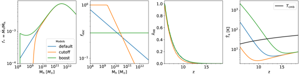
The precise properties of high-redshift galaxies, including their abundance and spectral properties, remain largely unknown, leaving some freedom in the choice of astrophysical parameters. To explore the dependency of our conclusions on astrophysical assumptions, we will perform our analysis for three different benchmark source models, called cutoff, default, and boost, which were introduced in [56, 37]. These three models are characterized by different stellar-to-halo relation , all of which result in UV luminosity functions consistent with current high redshift data [57, 58, 59, 60, 61, 62, 63, 64, 65, 66, 67, 68, 69, 70]. Specifically, the cutoff, default, and boost models feature a suppression, a power-law behavior, and an enhancement of star formation efficiency at small halo masses, respectively. We have tuned the escape fraction of ionizing photons in each model so that they achieve similar reionization history, consistent with observations [71, 72, 73, 74, 75, 76, 77, 78, 79, 80, 81, 82, 83]. Additionally, the normalization of the galactic X-ray spectrum varies between the models, resulting in distinct temperature evolution. The cutoff, default, and boost models exhibit a late, moderate, and early rise of the IGM temperature, respectively.
In Fig. 1, we plot the stellar-to-halo function in the left-most panel, the escape fraction in the second panel, the reionization history (z) in the third panel, and the evolution of the kinetic temperature in the right-most panel, for the cutoff, default, and boost models represented in orange, blue, and green colors, respectively. The halo catalogs and dark-matter density fields used in this study were obtained with the -body code, Pkdgrav3 [84], in a 147 cMpc cosmological box, with dark matter particles, resulting in a minimum halo mass of . The density fields and halo catalogs are saved every 10 Myr between and 6.
III Can we treat separately the EoR and the cosmic dawn?
The evolution of the 21cm signal is governed by three distinct mechanisms: the coupling of the spin temperature to the kinetic temperature induced by Lyman- photons, the heating of the gas mainly due to X-rays photons, and the growth and percolation of ionized bubbles produced by ionizing photons. These processes lead to the characteristic absorption trough in the global signal and the three-peak structure of the large-scale 21cm power spectrum [e.g. 87, 46, 88, 89].
While these mechanisms typically operate at different epochs, their effects overlap. For instance, rare and small ionized bubbles are already present during the epoch of Lyman- coupling and heating. Moreover, the universe may not be uniformly heated during the EoR, when ionization fluctuations dominate the signal. This raises questions about the impact of ionization on the cosmic dawn and vice versa.
A very common approximation in the literature is to separate the signals from the cosmic dawn and the epoch of reionization. Studies focusing on the reionization process often neglect potential fluctuation of the spin temperature [90, 91, 92, 32, 93, 94, 95] to simplify the analysis. A similar trick is often done in studies investigating the cosmic dawn where the reionization bubbles are often neglected [96, 97, 98, 35, 99].
In what follows, we investigate the validity of treating the epoch of cosmic dawn separately from the epoch of reionization. First, we investigate the impact of neglecting reionization and assuming a fully neutral universe during cosmic dawn (Sec. III.1). Then, we examine the saturated spin temperature assumption, which assumes a universe fully heated above the CMB temperature during the EoR (Sec. III.1).
III.1 Ignoring reionization during cosmic dawn
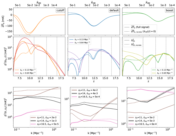
To investigate the impact of reionization on the 21cm signal, we use our simulation boxes of , , , and to generate a set of brightness temperature boxes where the ionization fraction () is assumed to be uniformly equal to 0. We label them with the subscript “no reio”. For the three benchmark models, we measure the global signal and power spectrum from these simulation boxes and compare them to the corresponding fiducial quantities. The results of this analysis are displayed in Fig. 2 for the redshift range . Dashed lines represent the “no reio” case, while solid lines show the full signal. The three columns correspond to the three models cutoff, default, and boost, from left to right, respectively.
In the upper row of Fig. 2, we plot the global signal . For all three models, the lines agree at the sub-percent level when . For , significant differences start to appear between the global signal predictions with and without ionized bubbles. Notably, we find these differences to be larger than in all three models. For instance when , we observe differences that are larger than . This is due to the non-zero correlations between the fields that compose the brightness temperature . We will further discuss this issue in Sec. IV.2.
In the second row of Fig. 2, we show the 21cm dimensionless power spectra as a function of redshift. We thereby focus on the two k-modes and , distinguished by different colours. The third row illustrates as a function of co-moving Fourier mode at three different redshifts and 16.5, which roughly cover the heating and Lyman- dominated regime in our models. They furthermore correspond to the redshift values where we currently have upper limits from PAPER [85] and MWA [86].
Examining the power spectra, we note that the differences between the “no reio” and the full signal appear at earlier redshifts compared to the global signal. They also vary substantially across the three models. We find that above the threshold , assuming a fully neutral universe leads to a bias of up to an order of magnitude in the power spectrum. This bias manifests as a suppression or an enhancement, depending on the source model. In the cutoff model, the presence of ionized bubbles enhances the 21cm power spectrum during the EoR, by creating a strong contrast between ionized regions with no signal () and cold regions with negative signal (). In contrast, in both the default and boost models, the IGM is significantly heated when . Thus, including ionized bubbles in these models decreases the 21cm power spectrum during the EoR by suppressing the peaks of the matter density field.
Focusing on the regime with (where less than five percent of the Universe is ionized) we find that the power spectra still differ by up to a factor of . This is best visible in the bottom row of Fig. 2 where all power spectra are at an ionization fraction below . The differences between the dashed and solid lines highlight the significant impact of the first ionized bubbles even if they occupy only a very subdominant fraction of the simulation volume.
At epochs characterized by , the influence of reionization on the power spectrum diminishes but remains visible. Overall, neglecting reionization in this regime tends to amplify the power spectrum, as revealed by the pink and black lines in the lower row of Fig. 2. In the default model, the impact is less pronounced but still noticeable, affecting the power spectrum by up to and at large and small scales, respectively. Finally, in the boost model, the large-scale power spectrum experiences a shift of a few percent, while small scales are impacted by up to .
It is worth noting that a fixed ionization fraction has a variable impact on the 21cm power spectrum depending on the astrophysical model. For instance, reaches at in the cutoff model, and at in the default and boost models. As visible from the global signals displayed in Fig. 4, the Lyman- coupling is more advanced at these stages in the latter two models compared to the former. The more advanced the UV coupling, the more abundant the absorption regions (), and the smaller the effect of the rare ionized bubbles on the power spectrum. Consequently, a larger fraction of regions in absorption is suppressed by ionized pixels in the cutoff model compared to the boost and default models.
We conclude that neglecting reionization during cosmic dawn when may result in an enhancement of the signal, increasingly more pronounced towards small scales. As indicated in the bottom panels of Fig. 2, the amplitude of this enhancement factor varies depending on the value of the ionization fraction and the astrophysical parameters. This shows the importance of including the modeling of the reionization process for future analysis focused on the epoch of Lyman- coupling and heating. Future studies aiming to constrain regions of the parameter space with cosmic dawn upper limits on the 21cm power spectrum may yield biased results if their modeling pipeline overlooks reionization.
III.2 Ignoring cosmic dawn during reionization
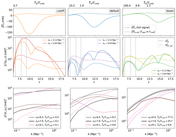
We now turn our attention towards the epoch of reionization (EoR), investigating the effect of temperature and Lyman- fluctuations on the signal. A common approximation consists of assuming a saturated spin temperature, i.e. the IGM being fully heated well above the CMB temperature during the whole EoR period. As in the previous subsection, we generate a set of boxes labeled (standing for “saturated”) for which . Then, we compute from these boxes the power spectrum and global signal which we compare to the true signal. Our findings are displayed in Fig. 3. The three columns again correspond to the three models, cutoff, default, and boost (from left to right). The dashed and solid lines represent the signals with and without saturated spin temperature, respectively.
In the top row of Fig. 3 we plot the global signal for the two cases. Not surprisingly, the saturated case only agrees with the full calculation when the gas temperature becomes significantly larger than the CMB temperature (see top axis showing the temperature ratio). Below differences start to become visible and below the two curves start to deviate strongly.
Similar conclusions can be drawn from the second row of Fig. 3, where we depict the 21cm power spectra as a function of redshift, at two different scales and . There is no well-delimited period in redshift where the saturated case yields results in agreement with the full calculation. Only in the boost model are the two lines close together for redshifts below 10. However, a closer inspection still reveals differences between 5 and 20 percent. For the default and the cutoff model, the “saturated” and true results are substantially different, even at late stages of reionization.
In the third row of Fig. 3, we display as a function of comoving Fourier mode at three different redshifts and 9.1. These redshifts are selected to be in the regime where reionization is believed to have occurred. They correspond to the redshift values from the current upper limits of MWA [100], HERA [29] and LOFAR [101], respectively. The differences between the saturated case and the full calculation lie between about 5 percent in the best case and 2-3 orders of magnitude in the worst.
The cutoff model corresponds to an example of cold reionization where remains below 1 across all redshifts. Therefore, the assumption of a saturated spin temperature is trivially not fulfilled and, hence, there is a very strong disagreement between the saturated and the full cases in Fig. 3. Even though Ref. [29] seems to indicate that cold reionization is disfavored, we have compared our cutoff model and find it below all the available upper limits.
In the default and boost models, more efficient X-ray heating drive the IGM temperature above before . In these two models, the saturated and full global signal calculations agree to better than once the fraction goes above 10. In the power spectrum, on the other hand, differences of order remain as long as . At the errors due to the saturated spin temperature assumption is typically between 20 and 50 percent.
In summary, our analysis shows that a true saturation of the spin temperature is only reached at and above. Below this ratio, neglecting fluctuations in the temperature and the Lyman- coupling yields errors of 10% or more on the 21cm power spectrum (a number that is strongly rising towards smaller values of ). For our three benchmark models, the condition of is never fulfilled during the EoR epoch. Although other models may have a regime where rises above 100, we cannot know if such a model is realised in nature before we measure the signal. We therefore conclude that assuming a saturated spin temperature is not an adequate strategy for predicting the 21cm signal.
IV Testing the perturbative approach
To bypass the computational cost of grid-based methods, and efficiently explore the vast astrophysical and cosmological parameter space, analytical techniques have been developed to compute the 21cm global signal and power spectrum within a matter of seconds, without modeling the full cosmological fluctuations of on a grid [102, 103, 42, 104, 105, 106, 35, 99, 107, 12]. These methods are rooted in a perturbative treatment of the field, and should not be confused with analytical methods based on an effective bias expansion of the signal [108, 109].
In this section, we investigate the accuracy of the perturbative approach for computing the 21cm signal. First, we describe the building blocks of the approach in Sec. IV.1. Then, we use our simulation boxes to reproduce the predictions of the perturbative approach, and compare them with the actual signal. We perform this test for our three benchmark models, examining the global signal in Sec. IV.2 before turning to the power spectrum in Sec. IV.3.
IV.1 The perturbative approach for 21cm
The core idea of the perturbative approach for the 21cm signal involves expressing the perturbation as a sum and product of individual perturbations arising from the matter, the ionization fraction, the kinetic temperature, and the Lyman- coupling coefficient fields. This decomposition is achieved through a Taylor expansion (as detailed in Sec. IV.1.2), and by neglecting high-order products of these fields (as described in Sec. IV.1.3). Subsequently, the 21cm power spectrum is obtained as a sum of auto and cross power spectra of these individual fields (see Sec. IV.1.4). These spectra can then be computed using various methods.
IV.1.1 Decomposition of into individual components
The fluctuations of are sourced by four space and time-dependent fields: , , and , representing the fractional perturbations of the , , , and the matter field, respectively. Accordingly, Eq. (1) can be reformulated as follows:
| (10) |
with
| (11) |
where the horizontal bars above letters designate spatially averaged quantities and where the -factors are given by , and only depend on redshift. Note that there is no assumption underlying Eq. (10), the equality is exact.
IV.1.2 The Taylor expansion approximation
To move forward and obtain a simpler expression for , the and fields are replaced by their Taylor series truncated at order 1. One then obtains
| (12) |
| (13) |
with and . Note that Eq. (12) and Eq. (13) are valid whenever
| (14) |
The Taylor expansion transforms the expression of into
| (15) |
with
| (16) |
Eq. (15) corresponds to a multivariate polynomial function of the 4 individual perturbation fields. It is the starting point to compute perturbatively. Note that being an approximation of the true field, it may lead to inaccurate results, especially near the center of halos where and may deviate significantly from their mean values, rendering the conditions of Eq. (14) invalid. Sec. IV.3 will further explore this issue.
IV.1.3 Linearity: neglecting high-order perturbations in , , and
Eq. (15) contains 16 individual products of fluctuations, which would lead to 16 + = 136 auto and cross terms when computing the power spectrum of . Therefore, it is critical to a priori neglect some of these terms. Since by construction is of order , the perturbations in must be kept to non-linear order. In previous studies such as [104, 12], every term including more than two perturbations in either , , or was discarded. This assumption was supported quantitatively by measuring the standard deviations of these three fields, which remain below one. This approach yields a more manageable expression for , which we indicate with the subscript “nl,r”:
| (17) |
IV.1.4 Final perturbative expression for the power spectrum
Moving forward with Eq. (17), we obtain the final decomposition for the 21cm power spectrum:
| (18) |
with
| (19) |
| (20) |
| (21) |
We isolated the higher-order contributions arising from matter () and ionization () perturbations, into for convenience. Note that all the individual terms above are power spectra of perturbative quantities , , , , including the pre-factors. For instance, is defined as the Fourier transform of . We refer to [110] for a more detailed study of these higher-order terms. The last three equations are the building blocks of the analytical approach for the 21cm power spectrum. We will test their validity in Sec. IV.
IV.2 Global Signal
The spatially averaged brightness temperature can be used to constrain both the cosmological and the astrophysical parameters. It is experimentally very challenging to measure, but several single-dish experiments currently attempt to detect the global 21cm signal during cosmic dawn and reionization [111, 112, 113, 114, 115, 116]. The EDGES detection [117], although being highly debated and even excluded at confidence by the SARAS3 experiment [118], triggered the community to explore the rich constraints that can be extracted from the global signal [see e.g. 119, 120, 121, 122, 123, 124, 125, 126]. Therefore, it is crucial to have at our disposal reliable and computationally efficient tools to predict the global signal.
Analytical codes such as ARES[105], HMreio[12] or ZEUS[99] can predict the global 21cm signal in a mere second. They compute the global signal based on the average quantity of the mean ionization fraction , the mean temperature of the gas , and the average Lyman- coupling coefficient . Therefore, they determine the quantity , as defined in Eq. 16. These methods implicitly assume that the mean of the product of several fields equals the product of their means, such that (Eq. 10), and that the mean of the fields and can be computed via the mean quantities and , such that . Combining these two assertions leads to .
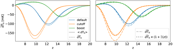
In the left-hand panel of Fig. 4, we display , and , computed from our simulation maps, as dashed and solid lines. The default, cutoff, and boost models are represented in blue, orange, and green colors. We observe a noticeable discrepancy between these two quantities. Across all the models, we find a relative error of about 10 around the dip of the absorption trough. In the EoR period (where the signal may be observed in emission) the relative error can reach a factor of 2. In terms of absolute error (expressed in mK) the largest values are found around the dip of the absorption trough, with values of 15, 10, and 5 mK for the cutoff, default, and boost models, respectively.
In the right-hand panel of Fig. 4, we show the quantity as dash-dotted line. is computed in a similar way than , but using the mean of the individual quantities and instead of and . Compared to , we find an even more pronounced discrepancy of order of . The difference between and is due to the fact that , and , while the difference between and arises from the fact that the mean of the product of multiple fields is not the product of their means.
We can understand the connection between and the actual global signal by taking the spatial average of equation Eq. (10). Ignoring all terms with more than 2 delta-terms we obtain
| (22) |
with
| (23) |
where denotes the covariance of the two fields , and . We calculate directly from our simulation boxes, as the spatial average of the product of two fields. depends only on redshift and is a sum of 6 different terms. In the right panel of Fig. 4, we plot the quantity . We observe that it provides a very good approximation of the true global signal, reducing the relative error around the dip of the absorption trough to below .
In summary, we find that analytical techniques to compute the 21cm global signal from the average of the individual fields lead to a error on the signal around the dip of the absorption trough. This is primarily caused by the fact that non-zero correlations between the fields are neglected. We provide a method to obtain accurate results with analytical models provided they can calculate the covariance between the individual fields.
IV.3 Power spectrum
In this section, we test and discuss the validity of the perturbative approach to compute the 21cm power spectrum based on the decomposition of into individual components (Eq. 18), and described in Sec. IV.1. Using the individual , , , boxes for our three astrophysical models, we compute the various auto and cross power spectra appearing in Eq. (19,20,21). This allows us to estimate the relevance of each term and examine the accuracy of the perturbative approach to model the 21cm power spectrum.
We begin by testing the performance of the linear prediction , defined in Eq. (19). This first approximation assumes full linearity of all the individual fields , , , . Note that here, ”linearity” refers to the assumption that perturbations are on average small, allowing us to neglect products of more than two terms in the decomposition. Under this assumption, reduces to Eq. (17) without the last three higher-order terms involving the perturbation. This approximation is known to be inaccurate during the EoR, due to the non-linearity of the ionization fraction field [110, 94], but has not been properly tested during cosmic dawn, and serves as the starting expression upon which we will add corrections.
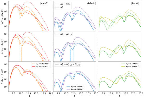
Using our simulated boxes, we compute the 10 terms present in Eq. (19) and subsequently calculate . In the three upper panels of Fig. 5, we plot the true dimensionless 21cm power spectrum computed from the -maps (solid lines) next to the linear prediction (dashed lines). The spectra are displayed at two different scales k = 0.13 and 0.64 Mpc-1. The cutoff, default, and boost models are represented in the leftmost, central, and rightmost panels, respectively.
For the three models, the linear approximation performs poorly over the whole range of redshifts. As expected, the match is better at the largest scale k=0.13 Mpc-1. Overall, the linear theory tends to overpredict the clustering signal. This overestimation is of the order of factor 2-3 for the larger scales (k=0.13 Mpc-1) going up to a factor 5-10 for the smaller scales (k=0.64 Mpc-1).
In the following, we will comment in more detail on the differences visible during both the cosmic dawn and the EoR. We will furthermore investigate to what extent higher-order terms can improve the result.
IV.3.1 The epoch of reionization
The EoR manifests itself as a peak in the 21cm power spectrum, visible between redshift and in our three models. The failure of linear theory is well expected in this regime because the field is known to have fluctuations of order unity. This issue was already addressed in the literature [110, 94] and solved by including higher-order products in to the decomposition. However, these studies investigated the contribution from higher-order terms assuming a saturated spin-temperature, thereby ignoring higher-order contributions arising from the temperature fluctuations. We perform the same kind of analysis but including temperature fluctuations. Namely, we check if the inclusion of the higher-order contributions in the matter () and reionization () fields (contained in Eq. 20) suffice to recover the true 21cm power spectrum during reionization.
Using our boxes of and , we compute the three extra terms contained in Eq. (20), and add this correction to the linear prediction. The result (denoted as ) is shown in the second row of Fig. 5. For the default and boost models a clear improvement can be observed. With the correction, the reionization peak is now accurately recovered in the both models. In the cutoff model, on the other hand, the higher order terms in and do not improve the fit with respect to the linear case. This is caused by the fact that the reionization and temperature peaks are merged in this model, strongly suggesting that at least the temperature fluctuations remain important until the late stages of reionization.
In the three bottom panels of Fig. 5, we show , the 21cm power spectrum consisting of all linear terms plus all the 24 higher-order contributions arising from perturbations, as defined in Eqs. (20, 21). The result of this decomposition is now in very good agreement with the true signal. Not only the default and boost but also the cutoff model now show a reasonable match with respect to the true result, at least for the reionization epoch at .
IV.3.2 Lyman- coupling and heating
Let us now turn our focus to the cosmic dawn, i.e., the heating and Lyman- coupling epochs which are taking place between redshift and 10 in our scenarios. Comparing the dashed curves in the upper row with the ones in the middle and bottom rows of Fig. 5, we note that the inclusion of all 24 higher-order contributions in results in a clear improvement of the model prediction, driving down the excess power predicted by linear theory. However, a significant mismatch persists. The 21cm power spectrum is still overestimated by up to a factor of 2 at k=0.13 Mpc-1 around both the heating and the Lyman- peaks across all three models. At the k=0.64 Mpc-1, the mismatch is more pronounced, reaching up to a factor 3-5 in the cutoff, default and boost models.
The next logical option to investigate is the influence of the remaining higher-order contributions to Eq. (15). We tested this possibility, finding a significantly worse match to the true signal once all higher-order terms are included. The observed mismatch is mainly driven by the extreme peaks produced by the cross-field. Our investigation suggests that the remaining difference between and visible in the bottom row of Fig. 5 is not due to missing higher-order contributions from the Lyman- and fields. In what follows, we will demonstrate that the error is instead caused by the Taylor expansion of the and fields which can produce very wrong results for the rare pixels where the perturbation criterion breaks down.
IV.3.3 Break-down of perturbation theory due to highly non-Gaussian distributions
In this section, we argue that the failure to correctly capture the 21cm power spectrum with the perturbative approach is caused by a diverging Taylor series at rare peaks where the fields exceed unity. To demonstrate this, let us focus on the first-order Taylor series expansion and written in Eqs. (12-13). These expansion terms are only valid for regions where the temperature and Lyman- coupling fields stay well below certain values (i.e. where Eq. 14 is satisfied). Since the and maps are constructed by the overlap of multiple profiles centered on halos, they can reach high values in the vicinity of halo centers. In these regions, both and predict very strong peaks while the true and cannot exceed one by definition. These artificial peaks contaminate the power spectrum up to large scales ( Mpc-1) and are at the origin of the differences between the power spectra of and . They form even when the standard deviation of the field is well below unity because the fields are non-Gaussian in nature and feature a tail going to high values.
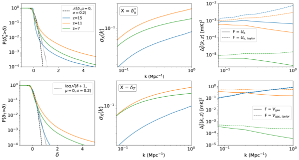
To support this last assertion, we measure the power spectra of , , and from our maps. We compare these quantities to the scale-dependent variance and the cumulative probability distribution of the fields and . We define the scale-dependent variance as , with the X field smoothed over top-hat kernels of radius R, and . The cumulative distribution function of a field is computed according to:
| (24) |
with representing the probability that takes the values , computed from the simulations boxes. The quantity informs us of the fraction of pixels with values exceeding a threshold .
We show our results in Fig. 6 for the default model only, as our findings are similar among the three models. The color coding is different than in the previous plots. The blue, orange, and green colors correspond to three different redshifts, , respectively. The first row focuses on the properties of the field, and the differences between the power spectrum of and , while the second row focuses on the properties of the field, and the differences between and . The first two columns show the cumulative distribution functions and standard deviations of and , in the upper and lower panels, respectively. The solid and dashed black lines visible in the leftmost panels represent the distribution functions of a normal and log-normal field with standard deviation . The third column compares the power spectra of and , and of and , in the upper and lower panel, respectively.
As visible in the third column of Fig. 6, there is an offset between the power spectra of and and of and . This mismatch increases towards small scales and is at the origin of the discrepancy between and observed in the middle upper panel of Fig. 5. Specifically at redshift , exceeds by a factor of 2 at k=0.13 Mpc-1 and 5 at k=0.64 Mpc-1. This discrepancy is equivalent to the deviation between and . The same conclusions hold at around the heating peak where the mismatch between the spectra of and is of a similar magnitude to the offset between and .
The leftmost panels of Fig. 6 demonstrate that and both present a heavy tail distribution, significantly deviating from a Gaussian or a log-normal field, and characterized by a significantly high fraction of pixels reaching high values . This distribution of high peaks is correlated to the error on the power spectrum induced by the Taylor series of and , but this relation is non-trivial. For instance, at redshift , the field is close to a log-normal with variance , as visible in the lower left panel of Fig. 6. At this redshift, the Taylor expansion is a valid approximation and exhibits a Fourier spectrum converged with its fiducial value, as indicated by the overlap of the solid and dashed blue curve in the lower right panel of Fig. 6. At other redshifts, where the high tail of the distribution flattens, we observe a divergence of compared to .
We conclude that despite the individual fields having a variance well below unity, they cannot be treated perturbatively due to their strongly non-Gaussian nature. The presence of strong peaks in the Lyman- and temperature fields leads to an overestimation of power within the perturbative approach. This bias originates from the invalidity of the Taylor series expansion around the peaks of the individual fields.
V Conclusions
Radio interferometers such as the Square Kilometre Array (SKA) will observe the 21cm signal from the neutral hydrogen during the cosmic dawn and the Epoch of reionization. Given the high complexity of coupled hydrodynamical radiative transfer computations, many calculations rely on simplifications and approximations to simulate the 21cm global signal and power spectrum. In this paper, we investigate the validity of a number of approximations commonly made in the literature.
Our analysis is conducted with the one-dimensional radiative-transfer code BEoRN [37] which uses an -body simulation as input and models the Lyman- coupling, X-ray heating, and the reionization process on a grid painting luminosity profiles around halo centres. The code provides cosmological boxes of the ionized hydrogen fraction (), the kinetic temperature of the gas (), the Lyman- coupling coefficient (), and the total differential brightness temperature (). We use these simulation boxes to mimic the predictions of various approximations and compare them to the true signal. In order to quantify the sensitivity of our results with respect to the astrophysical modeling, we investigate the three source models cutoff, default, and boost which differ in their stellar-to-halo mass and UV escape fractions for small galaxies (see Fig. 1 and corresponding text).
As a first step, we test the assumption of ignoring reionization bubbles when investigating the cosmic dawn, i.e. the epoch of Lyman- coupling and heating of the neutral gas. We show that disregarding reionization during cosmic dawn has an impact on the 21cm power spectrum up to very high redshifts. Even at early periods when the mean ionization fraction is well below the percent level, order deviations from the true power spectrum can occur in the relevant regime of Mpc-1.
Next, we investigate the very common assumption of a saturated spin temperature during reionization. This corresponds to ignoring all effects from the heating and the Lyman- coupling period during the reionization process. We find that for all three astrophysical source models considered here, effects from reionization cannot be safely decoupled from the cosmic dawn as the ratio of the mean neutral gas and CMB temperatures () always stays below 100. Even in the late regime where the mean temperature ration may go to , the assumption of a saturated spin temperature still leads to errors on the 21cm power spectrum of 10-20 %. This error grows substantially to about an order of magnitude when moving to the regime of . We conclude that the conditions for true spin saturation are hardly ever satisfied for realistic astrophysical source models.
As a next step, we examine the common approximation of calculating the global differential brightness temperature from the mean of the individual fields that compose the signal. We compare this calculation to the true global signal measured by averaging the -signal from the simulation box. Our analysis reveals a bias of approximately around the dip of the absorption trough in all three astrophysical source models. This error can be reduced when the correlations between the fields are accounted for. We propose a method to include the covariances from the individual clustering terms so that the true signal can be recovered to good precision.
Finally, we analyze the accuracy of the perturbative approach for computing the 21cm power spectrum. This method is based on a decomposition of the total fluctuations into a series of individual perturbations from the Lyman-, temperature, gas density, and ionization components. This decomposition is obtained by replacing certain components of the field with their Taylor series truncated to first order, and by neglecting high-order products of individual perturbations. For the epoch of reionization (EoR) we demonstrate (i) the necessity of including higher-order terms in the matter and ionization fields next to the standard linear terms, and (ii) the non-negligible contribution of higher-order terms in the temperature field for models where the epoch of heating overlaps with reionization. A similar study was performed in Refs. [110, 94], however, without including the impact of temperature and Lyman- perturbations.
Regarding the epoch of cosmic dawn, the linear perturbation approach overestimates the 21cm power spectrum during Lyman- coupling and heating by up to an order of magnitude. Including higher-order terms improves the situation somewhat, but differences of a factor of 2-3 remain. We attribute this remaining error to the highly non-Gaussian (heavy-tailed) distribution of the Lyman- and fields. Despite their variances being well below 1, these fields contain high peaks around large sources where the Taylor series expansion becomes very inaccurate.
We conclude that grid-based approaches are necessary to obtain accurate predictions of the total 21cm global signal and, more so, the power spectrum. Analytical approaches based on a perturbative series of individual perturbations remain very approximate, a fact that is mainly driven by the nonlinear dependence of the total 21cm signal to the Lyman- coupling and temperature fields (see Eq. 1).
Acknowledgements.
This work is supported by the Swiss National Science Foundation (SNF) via the grant PCEFP2_181157. Nordita is supported in part by NordForsk. We acknowledge the allocation of computing resources provided by the Swiss National Supercomputing Centre (CSCS) and National Academic Infrastructure for Supercomputing in Sweden (NAISS).References
- Mirocha et al. [2018] J. Mirocha, R. H. Mebane, S. R. Furlanetto, K. Singal, and D. Trinh, Unique signatures of Population III stars in the global 21-cm signal, Mon. Not. Roy. Astron. Soc. 478, 5591 (2018), arXiv:1710.02530 [astro-ph.GA] .
- Mebane et al. [2020] R. H. Mebane, J. Mirocha, and S. R. Furlanetto, The effects of population III radiation backgrounds on the cosmological 21-cm signal, Mon. Not. Roy. Astron. Soc. 493, 1217 (2020), arXiv:1910.10171 .
- Magg et al. [2022] M. Magg, I. Reis, A. Fialkov, R. Barkana, R. S. Klessen, S. C. O. Glover, L.-H. Chen, T. Hartwig, and A. T. P. Schauer, Effect of the cosmological transition to metal-enriched star formation on the hydrogen 21-cm signal, Mon. Not. Roy. Astron. Soc. 514, 4433 (2022), arXiv:2110.15948 [astro-ph.CO] .
- Kulkarni et al. [2017] G. Kulkarni, T. R. Choudhury, E. Puchwein, and M. G. Haehnelt, Large 21 cm signals from AGN-dominated reionization, Mon. Not. Roy. Astron. Soc. 469, 4283 (2017), arXiv:1701.04408 [astro-ph.CO] .
- Ventura et al. [2023] E. M. Ventura, A. Trinca, R. Schneider, L. Graziani, R. Valiante, and J. S. B. Wyithe, The role of Pop III stars and early black holes in the 21-cm signal from Cosmic Dawn, Monthly Notices of the Royal Astronomical Society 520, 3609 (2023), https://academic.oup.com/mnras/article-pdf/520/3/3609/50423328/stad237.pdf .
- Fialkov and Barkana [2019] A. Fialkov and R. Barkana, Signature of Excess Radio Background in the 21-cm Global Signal and Power Spectrum, Mon. Not. Roy. Astron. Soc. 486, 1763 (2019), arXiv:1902.02438 [astro-ph.CO] .
- Reis et al. [2020] I. Reis, A. Fialkov, and R. Barkana, High-redshift radio galaxies: a potential new source of 21-cm fluctuations, Mon. Not. Roy. Astron. Soc. 499, 5993 (2020), arXiv:2008.04315 [astro-ph.CO] .
- McQuinn et al. [2006] M. McQuinn, O. Zahn, M. Zaldarriaga, L. Hernquist, and S. R. Furlanetto, Cosmological parameter estimation using 21 cm radiation from the epoch of reionization, Astrophys. J. 653, 815 (2006), arXiv:astro-ph/0512263 .
- Mao et al. [2008] Y. Mao, M. Tegmark, M. McQuinn, M. Zaldarriaga, and O. Zahn, How accurately can 21 cm tomography constrain cosmology?, Phys. Rev. D 78, 023529 (2008), arXiv:0802.1710 [astro-ph] .
- Liu and Parsons [2016] A. Liu and A. R. Parsons, Constraining cosmology and ionization history with combined 21 cm power spectrum and global signal measurements, Mon. Not. Roy. Astron. Soc. 457, 1864 (2016), arXiv:1510.08815 [astro-ph.CO] .
- Kern et al. [2017] N. S. Kern, A. Liu, A. R. Parsons, A. Mesinger, and B. Greig, Emulating Simulations of Cosmic Dawn for 21 cm Power Spectrum Constraints on Cosmology, Reionization, and X-Ray Heating, Astrophys. J. 848, 23 (2017), arXiv:1705.04688 [astro-ph.CO] .
- Schneider et al. [2023] A. Schneider, T. Schaeffer, and S. K. Giri, Cosmological forecast of the 21-cm power spectrum with the halo model of reionization, Phys. Rev. D 108, 043030 (2023).
- Lopez-Honorez et al. [2019] L. Lopez-Honorez, O. Mena, and P. Villanueva-Domingo, Dark matter microphysics and 21 cm observations, Phys. Rev. D 99, 023522 (2019), arXiv:1811.02716 [astro-ph.CO] .
- Driskell et al. [2022] T. Driskell, E. O. Nadler, J. Mirocha, A. Benson, K. K. Boddy, T. D. Morton, J. Lashner, R. An, and V. Gluscevic, Structure formation and the global 21-cm signal in the presence of Coulomb-like dark matter-baryon interactions, Phys. Rev. D 106, 103525 (2022), arXiv:2209.04499 [astro-ph.CO] .
- Barkana et al. [2023] R. Barkana, A. Fialkov, H. Liu, and N. J. Outmezguine, Anticipating a new physics signal in upcoming 21-cm power spectrum observations, Phys. Rev. D 108, 063503 (2023), arXiv:2212.08082 [hep-ph] .
- Lopez-Honorez et al. [2017] L. Lopez-Honorez, O. Mena, S. Palomares-Ruiz, and P. Villanueva-Domingo, Warm dark matter and the ionization history of the Universe, Phys. Rev. D 96, 103539 (2017), arXiv:1703.02302 [astro-ph.CO] .
- Schneider [2018] A. Schneider, Constraining noncold dark matter models with the global 21-cm signal, Phys. Rev. D 98, 063021 (2018), arXiv:1805.00021 [astro-ph.CO] .
- Muñoz et al. [2021] J. B. Muñoz, S. Bohr, F.-Y. Cyr-Racine, J. Zavala, and M. Vogelsberger, ETHOS - an effective theory of structure formation: Impact of dark acoustic oscillations on cosmic dawn, Phys. Rev. D 103, 043512 (2021), arXiv:2011.05333 [astro-ph.CO] .
- Giri and Schneider [2022] S. K. Giri and A. Schneider, Imprints of fermionic and bosonic mixed dark matter on the 21-cm signal at cosmic dawn, Phys. Rev. D 105, 083011 (2022), arXiv:2201.02210 [astro-ph.CO] .
- van Haarlem et al. [2013] M. P. van Haarlem et al., LOFAR: The LOw-Frequency ARray, Astron. Astrophys. 556, A2 (2013), arXiv:1305.3550 [astro-ph.IM] .
- Tingay et al. [2013] S. J. Tingay et al., The Murchison Widefield Array: the Square Kilometre Array Precursor at low radio frequencies, Publ. Astron. Soc. Austral. 30, 7 (2013), arXiv:1206.6945 [astro-ph.IM] .
- DeBoer et al. [2017] D. R. DeBoer et al., Hydrogen Epoch of Reionization Array (HERA), Publ. Astron. Soc. Pac. 129, 045001 (2017), arXiv:1606.07473 [astro-ph.IM] .
- Paciga et al. [2013] G. Paciga, J. G. Albert, K. Bandura, T.-C. Chang, Y. Gupta, C. Hirata, J. Odegova, U.-L. Pen, J. B. Peterson, J. Roy, J. R. Shaw, K. Sigurdson, and T. Voytek, A simulation-calibrated limit on the HI power spectrum from the GMRT Epoch of Reionization experiment, Monthly Notices of the Royal Astronomical Society 433, 639 (2013), https://academic.oup.com/mnras/article-pdf/433/1/639/18722461/stt753.pdf .
- Kolopanis et al. [2019a] M. Kolopanis, D. C. Jacobs, C. Cheng, A. R. Parsons, S. A. Kohn, J. C. Pober, J. E. Aguirre, Z. S. Ali, G. Bernardi, R. F. Bradley, C. L. Carilli, D. R. DeBoer, M. R. Dexter, J. S. Dillon, J. Kerrigan, P. Klima, A. Liu, D. H. E. MacMahon, D. F. Moore, N. Thyagarajan, C. D. Nunhokee, W. P. Walbrugh, and A. Walker, A Simplified, Lossless Reanalysis of PAPER-64, Astrophys. J. 883, 133 (2019a), arXiv:1909.02085 [astro-ph.CO] .
- Ghara et al. [2020] R. Ghara et al., Constraining the intergalactic medium at z=9.1 using LOFAR Epoch of Reionization observations, Mon. Not. Roy. Astron. Soc. 493, 4728 (2020), arXiv:2002.07195 [astro-ph.CO] .
- Ghara et al. [2021] R. Ghara, S. K. Giri, B. Ciardi, G. Mellema, and S. Zaroubi, Constraining the state of the intergalactic medium during the epoch of reionization using mwa 21-cm signal observations, Monthly Notices of the Royal Astronomical Society 503, 4551 (2021).
- Greig et al. [2020] B. Greig, C. M. Trott, N. Barry, S. J. Mutch, B. Pindor, R. L. Webster, and J. S. B. Wyithe, Exploring reionization and high-z galaxy observables with recent multiredshift MWA upper limits on the 21-cm signal, Monthly Notices of the Royal Astronomical Society 500, 5322 (2020), https://academic.oup.com/mnras/article-pdf/500/4/5322/34908084/staa3494.pdf .
- Greig et al. [2021] B. Greig, A. Mesinger, L. V. Koopmans, B. Ciardi, G. Mellema, S. Zaroubi, S. K. Giri, R. Ghara, A. Ghosh, I. T. Iliev, et al., Interpreting lofar 21-cm signal upper limits at 9.1 in the context of high-z galaxy and reionization observations, Monthly Notices of the Royal Astronomical Society 501, 1 (2021).
- Abdurashidova et al. [2022] Z. Abdurashidova et al. (HERA), HERA Phase I Limits on the Cosmic 21 cm Signal: Constraints on Astrophysics and Cosmology during the Epoch of Reionization, Astrophys. J. 924, 51 (2022), arXiv:2108.07282 [astro-ph.CO] .
- Iliev et al. [2006] I. T. Iliev, B. Ciardi, M. A. Alvarez, A. Maselli, A. Ferrara, N. Y. Gnedin, G. Mellema, T. Nakamoto, M. L. Norman, A. O. Razoumov, et al., Cosmological radiative transfer codes comparison project–i. the static density field tests, Monthly Notices of the Royal Astronomical Society 371, 1057 (2006).
- Iliev et al. [2009] I. T. Iliev, D. Whalen, G. Mellema, K. Ahn, S. Baek, N. Y. Gnedin, A. V. Kravtsov, M. Norman, M. Raicevic, D. R. Reynolds, et al., Cosmological radiative transfer comparison project–ii. the radiation-hydrodynamic tests, Monthly Notices of the Royal Astronomical Society 400, 1283 (2009).
- Ghara et al. [2018] R. Ghara, G. Mellema, S. K. Giri, T. R. Choudhury, K. K. Datta, and S. Majumdar, Prediction of the 21-cm signal from reionization: comparison between 3D and 1D radiative transfer schemes, Monthly Notices of the Royal Astronomical Society 476, 1741 (2018), https://academic.oup.com/mnras/article-pdf/476/2/1741/24280051/sty314.pdf .
- Gnedin and Madau [2022] N. Y. Gnedin and P. Madau, Modeling cosmic reionization, Living Reviews in Computational Astrophysics 8, 3 (2022).
- Greig and Mesinger [2015] B. Greig and A. Mesinger, 21CMMC: an MCMC analysis tool enabling astrophysical parameter studies of the cosmic 21 cm signal, Mon. Not. Roy. Astron. Soc. 449, 4246 (2015), arXiv:1501.06576 [astro-ph.CO] .
- Schneider et al. [2021a] A. Schneider, S. K. Giri, and J. Mirocha, Halo model approach for the 21-cm power spectrum at cosmic dawn, Phys. Rev. D 103, 083025 (2021a).
- Monsalve et al. [2019] R. A. Monsalve, A. Fialkov, J. D. Bowman, A. E. Rogers, T. J. Mozdzen, A. Cohen, R. Barkana, and N. Mahesh, Results from edges high-band. iii. new constraints on parameters of the early universe, The Astrophysical Journal 875, 67 (2019).
- Schaeffer et al. [2023] T. Schaeffer, S. K. Giri, and A. Schneider, beorn: a fast and flexible framework to simulate the epoch of reionization and cosmic dawn, Monthly Notices of the Royal Astronomical Society 526, 2942 (2023), https://academic.oup.com/mnras/article-pdf/526/2/2942/51961266/stad2937.pdf .
- Aghanim et al. [2020] N. Aghanim et al. (Planck), Planck 2018 results. VI. Cosmological parameters, Astron. Astrophys. 641, A6 (2020), [Erratum: Astron.Astrophys. 652, C4 (2021)], arXiv:1807.06209 [astro-ph.CO] .
- Furlanetto [2006] S. Furlanetto, The Global 21 Centimeter Background from High Redshifts, Mon. Not. Roy. Astron. Soc. 371, 867 (2006), arXiv:astro-ph/0604040 .
- Mondal et al. [2020] R. Mondal, A. Fialkov, C. Fling, I. T. Iliev, R. Barkana, B. Ciardi, G. Mellema, S. Zaroubi, L. V. E. Koopmans, F. G. Mertens, B. K. Gehlot, R. Ghara, A. Ghosh, S. K. Giri, A. Offringa, and V. N. Pandey, Tight constraints on the excess radio background at z = 9.1 from LOFAR, Monthly Notices of the Royal Astronomical Society 498, 4178 (2020), https://academic.oup.com/mnras/article-pdf/498/3/4178/33787443/staa2422.pdf .
- He et al. [2023] Y. He, S. K. Giri, R. Sharma, S. Mtchedlidze, and I. Georgiev, Inverse gertsenshtein effect as a probe of high-frequency gravitational waves, arXiv preprint arXiv:2312.17636 (2023).
- Furlanetto et al. [2006] S. Furlanetto, S. P. Oh, and F. Briggs, Cosmology at Low Frequencies: The 21 cm Transition and the High-Redshift Universe, Phys. Rept. 433, 181 (2006), arXiv:astro-ph/0608032 .
- Mesinger et al. [2011] A. Mesinger, S. Furlanetto, and R. Cen, 21CMFAST: a fast, seminumerical simulation of the high-redshift 21-cm signal, MNRAS 411, 955 (2011), arXiv:1003.3878 [astro-ph.CO] .
- Santos et al. [2010] M. G. Santos, L. Ferramacho, M. Silva, A. Amblard, and A. Cooray, Fast large volume simulations of the 21-cm signal from the reionization and pre-reionization epochs, Monthly Notices of the Royal Astronomical Society 406, 2421 (2010).
- Hutter [2018] A. Hutter, CIFOG: Cosmological Ionization Fields frOm Galaxies, Astrophysics Source Code Library, record ascl:1803.002 (2018).
- Fialkov and Barkana [2014] A. Fialkov and R. Barkana, The rich complexity of 21-cm fluctuations produced by the first stars, Monthly Notices of the Royal Astronomical Society 445, 213 (2014).
- Semelin et al. [2007] B. Semelin, F. Combes, and S. Baek, Lyman-alpha radiative transfer during the Epoch of Reionization: contribution to 21-cm signal fluctuations, Astron. Astrophys. 474, 365 (2007), arXiv:0707.2483 [astro-ph] .
- Meriot and Semelin [2024] R. Meriot and B. Semelin, The loreli database: 21 cm signal inference with 3d radiative hydrodynamics simulations, Astronomy & Astrophysics 683, A24 (2024).
- Sokasian et al. [2001] A. Sokasian, T. Abel, and L. Hernquist, Simulating reionization in numerical cosmology, New Astronomy 6, 359 (2001).
- Mittal et al. [2023] S. Mittal, G. Kulkarni, and T. Garel, Radiative transfer of Lyman- photons at cosmic dawn with realistic gas physics https://doi.org/10.48550/arXiv.2311.03447 (2023), arXiv:2311.03447 .
- Maselli et al. [2003] A. Maselli, A. Ferrara, and B. Ciardi, Crash: a radiative transfer scheme, Monthly Notices of the Royal Astronomical Society 345, 379 (2003).
- Mellema et al. [2006a] G. Mellema, I. T. Iliev, M. A. Alvarez, and P. R. Shapiro, C2-ray: A new method for photon-conserving transport of ionizing radiation, New Astronomy 11, 374 (2006a).
- Hirling et al. [2023] P. Hirling, M. Bianco, S. K. Giri, I. T. Iliev, G. Mellema, and J.-P. Kneib, pyc2ray: A flexible and gpu-accelerated radiative transfer framework for simulating the cosmic epoch of reionization, arXiv preprint arXiv:2311.01492 (2023).
- Thomas et al. [2009] R. M. Thomas, S. Zaroubi, B. Ciardi, A. H. Pawlik, P. Labropoulos, V. Jelić, G. Bernardi, M. A. Brentjens, A. De Bruyn, G. J. Harker, et al., Fast large-scale reionization simulations, Monthly Notices of the Royal Astronomical Society 393, 32 (2009).
- Note [1] BEoRN is publicly available on: https://github.com/cosmic-reionization/BEoRN.
- Schneider et al. [2021b] A. Schneider, S. K. Giri, and J. Mirocha, Halo model approach for the 21-cm power spectrum at cosmic dawn, Phys. Rev. D 103, 083025 (2021b), arXiv:2011.12308 [astro-ph.CO] .
- McLure et al. [2013] R. J. McLure et al., A new multi-field determination of the galaxy luminosity function at z=7-9 incorporating the 2012 Hubble Ultra Deep Field imaging, Mon. Not. Roy. Astron. Soc. 432, 2696 (2013), arXiv:1212.5222 [astro-ph.CO] .
- McLeod et al. [2016] D. J. McLeod, R. J. McLure, and J. S. Dunlop, The z = 9-10 galaxy population in the Hubble Frontier Fields and CLASH surveys: the z = 9 luminosity function and further evidence for a smooth decline in ultraviolet luminosity density at z 8, Monthly Notices of the Royal Astronomical Society 459, 3812 (2016), https://academic.oup.com/mnras/article-pdf/459/4/3812/8192037/stw904.pdf .
- Livermore et al. [2017] R. C. Livermore, S. L. Finkelstein, and J. M. Lotz, Directly Observing the Galaxies Likely Responsible for Reionization, Astrophys. J. 835, 113 (2017), arXiv:1604.06799 [astro-ph.GA] .
- Ishigaki et al. [2018] M. Ishigaki, R. Kawamata, M. Ouchi, M. Oguri, K. Shimasaku, and Y. Ono, Full-data results of hubble frontier fields: Uv luminosity functions at z6–10 and a consistent picture of cosmic reionization, The Astrophysical Journal 854, 73 (2018).
- Atek et al. [2018] H. Atek, J. Richard, J.-P. Kneib, and D. Schaerer, The extreme faint end of the UV luminosity function at z 6 through gravitational telescopes: a comprehensive assessment of strong lensing uncertainties, Monthly Notices of the Royal Astronomical Society 479, 5184 (2018), https://academic.oup.com/mnras/article-pdf/479/4/5184/25207621/sty1820.pdf .
- Oesch et al. [2018] P. A. Oesch, R. J. Bouwens, G. D. Illingworth, I. Labbé, and M. Stefanon, The Dearth of z 10 Galaxies in All HST Legacy Fields—The Rapid Evolution of the Galaxy Population in the First 500 Myr, Astrophys. J. 855, 105 (2018), arXiv:1710.11131 [astro-ph.GA] .
- De Barros et al. [2019] S. De Barros, P. Oesch, I. Labbe, M. Stefanon, V. González, R. Smit, R. Bouwens, and G. Illingworth, The greats h + [o iii] luminosity function and galaxy properties at z 8: walking the way of jwst, Monthly Notices of the Royal Astronomical Society 489, 2355 (2019).
- Bowler et al. [2020] R. A. A. Bowler, M. J. Jarvis, J. S. Dunlop, R. J. McLure, D. J. McLeod, N. J. Adams, B. Milvang-Jensen, and H. J. McCracken, A lack of evolution in the very bright end of the galaxy luminosity function from z 8 to 10, Mon. Not. Roy. Astron. Soc. 493, 2059 (2020), arXiv:1911.12832 [astro-ph.GA] .
- Rojas-Ruiz et al. [2020] S. Rojas-Ruiz, S. L. Finkelstein, M. B. Bagley, M. Stevans, K. D. Finkelstein, R. Larson, M. Mechtley, and J. Diekmann, Probing the Bright End of the Rest-frame Ultraviolet Luminosity Function at z = 8-10 with Hubble Pure-parallel Imaging, Astrophys. J. 891, 146 (2020), arXiv:2002.06209 [astro-ph.GA] .
- Bouwens et al. [2021] R. J. Bouwens, P. A. Oesch, M. Stefanon, G. Illingworth, I. Labbé, N. Reddy, H. Atek, M. Montes, R. Naidu, T. Nanayakkara, E. Nelson, and S. Wilkins, New determinations of the uv luminosity functions from z 9 to 2 show a remarkable consistency with halo growth and a constant star formation efficiency, The Astronomical Journal 162, 47 (2021).
- Bouwens et al. [2022] R. Bouwens, G. Illingworth, P. Oesch, M. Stefanon, R. Naidu, I. van Leeuwen, and D. Magee, Uv luminosity density results at z¿8 from the first jwst/nircam fields: Limitations of early data sets and the need for spectroscopy (2022), arXiv:2212.06683 .
- Finkelstein et al. [2022] S. L. Finkelstein, M. B. Bagley, H. C. Ferguson, S. M. Wilkins, J. S. Kartaltepe, C. Papovich, L. Y. A. Yung, P. Arrabal Haro, P. Behroozi, M. Dickinson, D. D. Kocevski, A. M. Koekemoer, R. L. Larson, A. Le Bail, A. M. Morales, P. G. Perez-Gonzalez, D. Burgarella, R. Dave, M. Hirschmann, R. S. Somerville, S. Wuyts, V. Bromm, C. M. Casey, A. Fontana, S. Fujimoto, J. P. Gardner, M. Giavalisco, A. Grazian, N. A. Grogin, N. P. Hathi, T. A. Hutchison, S. W. Jha, S. Jogee, L. J. Kewley, A. Kirkpatrick, A. S. Long, J. M. Lotz, L. Pentericci, J. D. R. Pierel, N. Pirzkal, S. Ravindranath, J. Ryan, Russell E., J. R. Trump, G. Yang, R. Bhatawdekar, L. Bisigello, V. Buat, A. Calabro, M. Castellano, N. J. Cleri, M. C. Cooper, D. Croton, E. Daddi, A. Dekel, D. Elbaz, M. Franco, E. Gawiser, B. W. Holwerda, M. Huertas-Company, A. E. Jaskot, G. C. K. Leung, R. A. Lucas, B. Mobasher, V. Pandya, S. Tacchella, B. J. Weiner, and J. A. Zavala, CEERS Key Paper I: An Early Look into the First 500 Myr of Galaxy Formation with JWST, arXiv e-prints , arXiv:2211.05792 (2022), arXiv:2211.05792 [astro-ph.GA] .
- Donnan et al. [2022] C. Donnan, D. McLeod, J. Dunlop, R. McLure, A. Carnall, R. Begley, F. Cullen, M. Hamadouche, R. Bowler, D. Magee, H. McCracken, B. Milvang-Jensen, A. Moneti, and T. Targett, The evolution of the galaxy uv luminosity function at redshifts z 8 – 15 from deep jwst and ground-based near-infrared imaging, Monthly Notices of the Royal Astronomical Society 518 (2022).
- Harikane et al. [2023] Y. Harikane, M. Ouchi, M. Oguri, Y. Ono, K. Nakajima, Y. Isobe, H. Umeda, K. Mawatari, and Y. Zhang, A comprehensive study of galaxies at z 9–16 found in the early jwst data: Ultraviolet luminosity functions and cosmic star formation history at the pre-reionization epoch, The Astrophysical Journal Supplement Series 265, 5 (2023).
- Ouchi et al. [2010] M. Ouchi, K. Shimasaku, H. Furusawa, T. Saito, M. Yoshida, M. Akiyama, Y. Ono, T. Yamada, K. Ota, N. Kashikawa, M. Iye, T. Kodama, S. Okamura, C. Simpson, and M. Yoshida, Statistics of 207 ly emitters at a redshift near 7: Constraints on reionization and galaxy formation models, The Astrophysical Journal 723, 869 (2010).
- Mortlock et al. [2011] D. J. Mortlock, S. J. Warren, B. P. Venemans, M. Patel, P. C. Hewett, R. G. McMahon, C. Simpson, T. Theuns, E. A. Gonzáles-Solares, A. Adamson, S. Dye, N. C. Hambly, P. Hirst, M. J. Irwin, E. Kuiper, A. Lawrence, and H. J. A. Röttgering, A luminous quasar at a redshift of z = 7.085, Nature 474, 616 (2011).
- Ono et al. [2011] Y. Ono, M. Ouchi, B. Mobasher, M. Dickinson, K. Penner, K. Shimasaku, B. J. Weiner, J. S. Kartaltepe, K. Nakajima, H. Nayyeri, D. Stern, N. Kashikawa, and H. Spinrad, Spectroscopic confirmation of three z-dropout galaxies at z = 6.844–7.213: Demographics of ly emission in z 7 galaxies, The Astrophysical Journal 744, 83 (2011).
- Schroeder et al. [2012] J. Schroeder, A. Mesinger, and Z. Haiman, Evidence of Gunn–Peterson damping wings in high-z quasar spectra: strengthening the case for incomplete reionization at z 6–7, Monthly Notices of the Royal Astronomical Society 428, 3058 (2012), https://academic.oup.com/mnras/article-pdf/428/4/3058/18459892/sts253.pdf .
- Tilvi et al. [2014] V. Tilvi, C. Papovich, S. L. Finkelstein, J. Long, M. Song, M. Dickinson, H. C. Ferguson, A. M. Koekemoer, M. Giavalisco, and B. Mobasher, Rapid decline of ly emission toward the reionization era, The Astrophysical Journal 794, 5 (2014).
- Pentericci et al. [2014] L. Pentericci, E. Vanzella, A. Fontana, M. Castellano, T. Treu, A. Mesinger, M. Dijkstra, A. Grazian, M. Bradač, C. Conselice, S. Cristiani, J. Dunlop, A. Galametz, M. Giavalisco, E. Giallongo, A. Koekemoer, R. McLure, R. Maiolino, D. Paris, and P. Santini, New observations of z 7 galaxies: Evidence for a patchy reionization, The Astrophysical Journal 793, 113 (2014).
- Totani et al. [2016] T. Totani, K. Aoki, T. Hattori, and N. Kawai, High-precision analyses of Ly damping wing of gamma-ray bursts in the reionization era: On the controversial results from GRB 130606A at z = 5.91, Publications of the Astronomical Society of Japan 68, 10.1093/pasj/psv123 (2016), 15, https://academic.oup.com/pasj/article-pdf/68/1/15/7489339/psv123.pdf .
- Bañados et al. [2018] E. Bañados, C. Venemans, Bram P.and Mazzucchelli, E. P. Farina, F. Walter, F. Wang, R. Decarli, D. Stern, X. Fan, F. B. Davies, J. F. Hennawi, R. A. Simcoe, M. L. Turner, H.-W. Rix, J. Yang, D. D. Kelson, G. C. Rudie, and J. M. Winters, An 800-million-solar-mass black hole in a significantly neutral universe at a redshift of 7.5, Nature 553, 473 (2018).
- Mason et al. [2018] C. A. Mason, T. Treu, M. Dijkstra, A. Mesinger, M. Trenti, L. Pentericci, S. de Barros, and E. Vanzella, The universe is reionizing at z7: Bayesian inference of the igm neutral fraction using ly- emission from galaxies, The Astrophysical Journal 856, 2 (2018).
- Hoag et al. [2019] A. Hoag, M. Bradač, K. Huang, C. Mason, T. Treu, K. B. Schmidt, M. Trenti, V. Strait, B. C. Lemaux, E. Q. Finney, and M. Paddock, Constraining the neutral fraction of hydrogen in the igm at redshift 7.5, The Astrophysical Journal 878, 12 (2019).
- Ďurovčíková et al. [2020] D. Ďurovčíková, H. Katz, S. E. I. Bosman, F. B. Davies, J. Devriendt, and A. Slyz, Reionization history constraints from neural network based predictions of high-redshift quasar continua, Monthly Notices of the Royal Astronomical Society 493, 4256 (2020), https://academic.oup.com/mnras/article-pdf/493/3/4256/32920432/staa505.pdf .
- Jung et al. [2020] I. Jung, S. L. Finkelstein, M. Dickinson, T. A. Hutchison, R. L. Larson, C. Papovich, L. Pentericci, A. N. Straughn, Y. Guo, S. Malhotra, J. Rhoads, M. Song, V. Tilvi, and I. Wold, Texas Spectroscopic Search for Ly Emission at the End of Reionization. III. The Ly Equivalent-width Distribution and Ionized Structures at z ¿ 7, Astrophys. J. 904, 144 (2020), arXiv:2009.10092 [astro-ph.GA] .
- Bruton et al. [2023] S. Bruton, Y.-H. Lin, C. Scarlata, and M. J. Hayes, The universe is at most 88% neutral at z=10.6 (2023), arXiv:2303.03419 .
- Potter et al. [2017] D. Potter, J. Stadel, and R. Teyssier, Pkdgrav3: beyond trillion particle cosmological simulations for the next era of galaxy surveys, Computational Astrophysics and Cosmology 4, 2 (2017).
- Kolopanis et al. [2019b] M. Kolopanis, D. C. Jacobs, C. Cheng, A. R. Parsons, S. A. Kohn, J. C. Pober, J. E. Aguirre, Z. S. Ali, G. Bernardi, R. F. Bradley, C. L. Carilli, D. R. DeBoer, M. R. Dexter, J. S. Dillon, J. Kerrigan, P. Klima, A. Liu, D. H. E. MacMahon, D. F. Moore, N. Thyagarajan, C. D. Nunhokee, W. P. Walbrugh, and A. Walker, A Simplified, Lossless Reanalysis of PAPER-64, Astrophys. J. 883, 133 (2019b), arXiv:1909.02085 [astro-ph.CO] .
- Yoshiura et al. [2021] S. Yoshiura, B. Pindor, J. L. B. Line, N. Barry, C. M. Trott, A. Beardsley, J. Bowman, R. Byrne, A. Chokshi, B. J. Hazelton, K. Hasegawa, E. Howard, B. Greig, D. Jacobs, C. H. Jordan, R. Joseph, M. Kolopanis, C. Lynch, B. McKinley, D. A. Mitchell, M. F. Morales, S. G. Murray, J. C. Pober, M. Rahimi, K. Takahashi, S. J. Tingay, R. B. Wayth, R. L. Webster, M. Wilensky, J. S. B. Wyithe, Z. Zhang, and Q. Zheng, A new MWA limit on the 21 cm power spectrum at redshifts 13–17, Monthly Notices of the Royal Astronomical Society 505, 4775 (2021), https://academic.oup.com/mnras/article-pdf/505/4/4775/38828418/stab1560.pdf .
- Mesinger et al. [2013] A. Mesinger, A. Ferrara, and D. S. Spiegel, Signatures of x-rays in the early universe, Monthly Notices of the Royal Astronomical Society 431, 621 (2013).
- Ghara et al. [2015] R. Ghara, T. R. Choudhury, and K. K. Datta, 21 cm signal from cosmic dawn: imprints of spin temperature fluctuations and peculiar velocities, Monthly Notices of the Royal Astronomical Society 447, 1806 (2015).
- Mesinger et al. [2016] A. Mesinger, B. Greig, and E. Sobacchi, The evolution of 21 cm structure (eos): public, large-scale simulations of cosmic dawn and reionization, Monthly Notices of the Royal Astronomical Society 459, 2342 (2016).
- Mellema et al. [2006b] G. Mellema, I. T. Iliev, U.-L. Pen, and P. R. Shapiro, Simulating cosmic reionization at large scales – II. The 21-cm emission features and statistical signals, Monthly Notices of the Royal Astronomical Society 372, 679 (2006b), https://academic.oup.com/mnras/article-pdf/372/2/679/2986158/mnras0372-0679.pdf .
- Zahn et al. [2011] O. Zahn, A. Mesinger, M. McQuinn, H. Trac, R. Cen, and L. E. Hernquist, Comparison of reionization models: radiative transfer simulations and approximate, seminumeric models, Monthly Notices of the Royal Astronomical Society 414, 727 (2011), https://academic.oup.com/mnras/article-pdf/414/1/727/3838580/mnras0414-0727.pdf .
- Majumdar et al. [2014] S. Majumdar, G. Mellema, K. K. Datta, H. Jensen, T. R. Choudhury, S. Bharadwaj, and M. M. Friedrich, On the use of seminumerical simulations in predicting the 21-cm signal from the epoch of reionization, Monthly Notices of the Royal Astronomical Society 443, 2843 (2014), https://academic.oup.com/mnras/article-pdf/443/4/2843/6274877/stu1342.pdf .
- Hassan et al. [2016] S. Hassan, R. Davé, K. Finlator, and M. G. Santos, Simulating the 21 cm signal from reionization including non-linear ionizations and inhomogeneous recombinations, Monthly Notices of the Royal Astronomical Society 457, 1550 (2016), https://academic.oup.com/mnras/article-pdf/457/2/1550/2888816/stv3001.pdf .
- Georgiev et al. [2022] I. Georgiev, G. Mellema, S. K. Giri, and R. Mondal, The large-scale 21-cm power spectrum from reionization, Mon. Not. Roy. Astron. Soc. 513, 5109 (2022), arXiv:2110.13190 [astro-ph.CO] .
- Georgiev et al. [2024] I. Georgiev, A. Gorce, and G. Mellema, Constraining cosmic reionization by combining the kinetic Sunyaev–Zel’dovich and the 21cm power spectra, Monthly Notices of the Royal Astronomical Society 528, 7218 (2024), https://academic.oup.com/mnras/article-pdf/528/4/7218/56753860/stae506.pdf .
- Visbal et al. [2012] E. Visbal, R. Barkana, A. Fialkov, D. Starson, and C. Hirata, The signature of the first stars in atomic hydrogen at redshift 20, Nature 487, 70 (2012).
- Fialkov et al. [2012] A. Fialkov, R. Barkana, E. Visbal, D. Starson, and C. Hirata, The 21-cm signature of the first stars during the lyman-werner feedback era, Monthly Notices of the Royal Astronomical Society 432 (2012).
- Fialkov et al. [2013] A. Fialkov, R. Barkana, A. Pinhas, and E. Visbal, Complete history of the observable 21cm signal from the first stars during the pre-reionization era, Monthly Notices of the Royal Astronomical Society: Letters 437, L36 (2013), https://academic.oup.com/mnrasl/article-pdf/437/1/L36/56941277/mnrasl_437_1_l36.pdf .
- Muñoz [2023] J. B. Muñoz, An effective model for the cosmic-dawn 21-cm signal, Monthly Notices of the Royal Astronomical Society 523, 2587 (2023), https://academic.oup.com/mnras/article-pdf/523/2/2587/50524758/stad1512.pdf .
- Trott et al. [2020] C. M. Trott, C. H. Jordan, S. Midgley, N. Barry, B. Greig, B. Pindor, J. H. Cook, G. Sleap, S. J. Tingay, D. Ung, P. Hancock, A. Williams, J. Bowman, R. Byrne, A. Chokshi, B. J. Hazelton, K. Hasegawa, D. Jacobs, R. C. Joseph, W. Li, J. L. B. Line, C. Lynch, B. McKinley, D. A. Mitchell, M. F. Morales, M. Ouchi, J. C. Pober, M. Rahimi, K. Takahashi, R. B. Wayth, R. L. Webster, M. Wilensky, J. S. B. Wyithe, S. Yoshiura, Z. Zhang, and Q. Zheng, Deep multiredshift limits on Epoch of Reionization 21 cm power spectra from four seasons of Murchison Widefield Array observations, Monthly Notices of the Royal Astronomical Society 493, 4711 (2020), https://academic.oup.com/mnras/article-pdf/493/4/4711/32927265/staa414.pdf .
- Mertens et al. [2020] F. G. Mertens et al., Improved upper limits on the 21-cm signal power spectrum of neutral hydrogen at from LOFAR, Mon. Not. Roy. Astron. Soc. 493, 1662 (2020), arXiv:2002.07196 [astro-ph.CO] .
- Barkana and Loeb [2005] R. Barkana and A. Loeb, A Method for separating the physics from the astrophysics of high-redshift 21 cm fluctuations, Astrophys. J. Lett. 624, L65 (2005), arXiv:astro-ph/0409572 .
- Barkana and Loeb [2005] R. Barkana and A. Loeb, Detecting the Earliest Galaxies through Two New Sources of 21 Centimeter Fluctuations, Astrophys. J. 626, 1 (2005), arXiv:astro-ph/0410129 [astro-ph] .
- Pritchard and Furlanetto [2007] J. R. Pritchard and S. R. Furlanetto, 21 cm fluctuations from inhomogeneous X-ray heating before reionization, Mon. Not. Roy. Astron. Soc. 376, 1680 (2007), arXiv:astro-ph/0607234 .
- Mirocha [2014] J. Mirocha, Decoding the X-ray Properties of Pre-Reionization Era Sources, Mon. Not. Roy. Astron. Soc. 443, 1211 (2014), arXiv:1406.4120 [astro-ph.GA] .
- Raste and Sethi [2018] J. Raste and S. Sethi, An analytic formulation of the 21 cm signal from the early phase of the epoch of reionization, The Astrophysical Journal 860, 55 (2018).
- Mirocha et al. [2022] J. Mirocha, J. B. Muñoz, S. R. Furlanetto, A. Liu, and A. Mesinger, A galaxy-free phenomenological model for the 21-cm power spectrum during reionization, Mon. Not. Roy. Astron. Soc. 514, 2010 (2022), arXiv:2201.07249 [astro-ph.CO] .
- McQuinn and D’Aloisio [2018] M. McQuinn and A. D’Aloisio, The observable 21cm signal from reionization may be perturbative, Journal of Cosmology and Astroparticle Physics 2018 (10), 016.
- Qin et al. [2022] W. Qin, K. Schutz, A. Smith, E. Garaldi, R. Kannan, T. R. Slatyer, and M. Vogelsberger, Effective bias expansion for 21-cm cosmology in redshift space, Physical Review D 106, 123506 (2022).
- Lidz et al. [2007] A. Lidz, O. Zahn, M. McQuinn, M. Zaldarriaga, and S. Dutta, Higher Order Contributions to the 21 cm Power Spectrum, Astrophys. J. 659, 865 (2007), arXiv:astro-ph/0610054 .
- Sokolowski et al. [2015] M. Sokolowski, S. Tremblay, R. Wayth, S. Tingay, N. Clarke, P. Roberts, M. Waterson, R. Ekers, P. Hall, M. Lewis, M. Mossammaparast, S. Padhi, F. Schlagenhaufer, A. Sutinjo, and J. Tickner, Bighorns - broadband instrument for global hydrogen reionisation signal, Publications of the Astronomical Society of Australia 32 (2015).
- Singh et al. [2018] S. Singh, R. Subrahmanyan, U. Narayana Rao, M. Rao, G. Baragur, A. Raghunathan, R. Somashekar, and S. K.s, Saras 2: A spectral radiometer for probing cosmic dawn and the epoch of reionization through detection of the global 21 cm signal, Experimental Astronomy 45 (2018).
- de Lera Acedo et al. [2022] E. de Lera Acedo, D. I. L. de Villiers, N. Razavi-Ghods, W. Handley, A. Fialkov, A. Magro, D. Anstey, H. T. J. Bevins, R. Chiello, J. Cumner, A. T. Josaitis, I. L. V. Roque, P. H. Sims, K. H. Scheutwinkel, P. Alexander, G. Bernardi, S. Carey, J. Cavillot, W. Croukamp, J. A. Ely, T. Gessey-Jones, Q. Gueuning, R. Hills, G. Kulkarni, R. Maiolino, P. D. Meerburg, S. Mittal, J. R. Pritchard, E. Puchwein, A. Saxena, E. Shen, O. Smirnov, M. Spinelli, and K. Zarb-Adami, The REACH radiometer for detecting the 21-cm hydrogen signal from redshift z 7.5-28, Nature Astronomy 6, 984 (2022), arXiv:2210.07409 [astro-ph.CO] .
- Philip et al. [2019] L. Philip, Z. Abdurashidova, H. C. Chiang, N. Ghazi, A. Gumba, H. M. Heilgendorff, J. M. Jáuregui-García, K. Malepe, C. D. Nunhokee, J. Peterson, J. L. Sievers, V. Simes, and R. Spann, Probing radio intensity at high-z from marion: 2017 instrument, Journal of Astronomical Instrumentation 08, 1950004 (2019), https://doi.org/10.1142/S2251171719500041 .
- Price et al. [2018] D. C. Price, L. J. Greenhill, A. Fialkov, G. Bernardi, H. Garsden, B. R. Barsdell, J. Kocz, M. M. Anderson, S. A. Bourke, J. Craig, M. R. Dexter, J. Dowell, M. W. Eastwood, T. Eftekhari, S. W. Ellingson, G. Hallinan, J. M. Hartman, R. Kimberk, T. J. W. Lazio, S. Leiker, D. MacMahon, R. Monroe, F. Schinzel, G. B. Taylor, E. Tong, D. Werthimer, and D. P. Woody, Design and characterization of the Large-aperture Experiment to Detect the Dark Age (LEDA) radiometer systems, Monthly Notices of the Royal Astronomical Society 478, 4193 (2018), https://academic.oup.com/mnras/article-pdf/478/3/4193/25097057/sty1244.pdf .
- Monsalve et al. [2023] R. A. Monsalve, C. Altamirano, V. Bidula, R. Bustos, C. H. Bye, H. C. Chiang, M. Diaz, B. Fernandez, X. Guo, I. Hendricksen, E. Hornecker, F. Lucero, H. Mani, F. McGee, F. P. Mena, M. Pessoa, G. Prabhakar, O. Restrepo, J. L. Sievers, and N. Thyagarajan, Mapper of the igm spin temperature (mist): Instrument overview (2023), arXiv:2309.02996 .
- Bowman et al. [2018] J. D. Bowman, A. E. E. Rogers, R. A. Monsalve, T. J. Mozdzen, and N. Mahesh, An absorption profile centred at 78 megahertz in the sky-averaged spectrum, Nature (London) 555, 67 (2018), arXiv:1810.05912 [astro-ph.CO] .
- Singh et al. [2022] S. Singh, N. T. Jishnu, R. Subrahmanyan, N. Udaya Shankar, B. S. Girish, A. Raghunathan, R. Somashekar, K. S. Srivani, and M. Sathyanarayana Rao, On the detection of a cosmic dawn signal in the radio background, Nature Astronomy 6, 607 (2022), arXiv:2112.06778 [astro-ph.CO] .
- Mirocha and Furlanetto [2019] J. Mirocha and S. R. Furlanetto, What does the first highly-redshifted 21-cm detection tell us about early galaxies?, Mon. Not. Roy. Astron. Soc. 483, 1980 (2019), arXiv:1803.03272 [astro-ph.GA] .
- D’Amico et al. [2018] G. D’Amico, P. Panci, and A. Strumia, Bounds on dark-matter annihilations from 21-cm data, Phys. Rev. Lett. 121, 011103 (2018).
- Fialkov et al. [2018] A. Fialkov, R. Barkana, and A. Cohen, Constraining baryon–dark-matter scattering with the cosmic dawn 21-cm signal, Phys. Rev. Lett. 121, 011101 (2018).
- Hektor et al. [2018] A. Hektor, G. Hütsi, L. Marzola, M. Raidal, V. Vaskonen, and H. Veermäe, Constraining primordial black holes with the edges 21-cm absorption signal, Phys. Rev. D 98, 023503 (2018).
- Brandenberger et al. [2019] R. Brandenberger, B. Cyr, and T. Schaeffer, On the possible enhancement of the global 21-cm signal at reionization from the decay of cosmic string cusps, Journal of Cosmology and Astroparticle Physics 2019 (04), 020.
- Mitridate and Podo [2018] A. Mitridate and A. Podo, Bounds on dark matter decay from 21 cm line, Journal of Cosmology and Astroparticle Physics 2018 (05), 069.
- Wang and Zhao [2018] Y. Wang and G.-B. Zhao, Constraining the dark matter vacuum energy interaction using the edges 21 cm absorption signal, The Astrophysical Journal 869, 26 (2018).
- Mittal and Kulkarni [2022] S. Mittal and G. Kulkarni, Implications of the cosmological 21-cm absorption profile for high-redshift star formation and deep JWST surveys, Monthly Notices of the Royal Astronomical Society 515, 2901 (2022), https://academic.oup.com/mnras/article-pdf/515/2/2901/45212861/stac1961.pdf .