The expected kinematic matter dipole is robust against source evolution

Abstract

Recent measurements using catalogues of quasars and radio galaxies have shown that the dipole anisotropy in the large-scale distribution of matter is about twice as large as is expected in the standard $\Lambda$CDM model, indeed in any cosmology based on the Friedman-Lemaître-Robertson-Walker (FLRW) metric. This expectation is based on the kinematic interpretation of the dipole anisotropy of the cosmic microwave background, i.e. as arising due to our local peculiar velocity. The effect of aberration and Doppler boosting on the projected number counts on the sky of cosmologically distant objects in a flux-limited catalogue can then be calculated and confronted with observations. This fundamental consistency test of FLRW models proposed by Ellis & Baldwin (1984) was revisited by Dalang & Bonvin (2022) who argued that redshift evolution of the sources can significantly affect the expected matter dipole. In this note we demonstrate that the Ellis & Baldwin test is in fact robust to such effects, hence the $>5\sigma$ dipole anomaly uncovered by Secrest et al. (2021, 2022) remains an outstanding challenge to the $\Lambda$CDM model.

1 Introduction

The standard $\Lambda$CDM cosmological model describes a Universe in which small primordial inhomogeneities superimposed on a smooth background grow via gravitational instability over cosmic time. The background is defined by the FLRW metric of space-time that allows the evolution to be computed when the energy-momentum tensor is that of an ideal fluid. While this choice of metric was motivated by simplicity rather than observational evidence, its implication that the Universe should look homogeneous and isotropic to any comoving observer was promoted to the ‘Cosmological Principle’ (CP) (Milne, 1933). The validity of all conclusions that follow from interpreting data in the standard cosmological framework, including the inference of $\Lambda$ itself, rests on whether the CP holds for the real Universe.

We are not in fact comoving observers; we infer this from the observation of a dipole anisotropy in the Cosmic Microwave Background (CMB) which is interpreted as due to our peculiar velocity $\beta\sim 10^{-3}$ with respect to the rest frame in which the CMB is isotropic (Stewart & Sciama, 1967; Peebles & Wilkinson, 1968). This is called the ‘CMB frame’, and the CP implies that the large-scale distribution of matter should also be isotropic in this frame. Hence in order to interpret cosmological data in the standard $\Lambda$CDM framework, observables measured in the heliocentric frame are boosted to the CMB frame. This has shown good agreement with a wide range of data, moreover direct tests of homogeneity have so far supported the CP. For example counts-in-cells of quasars (e.g. Laurent et al., 2016) indicate homogeneity is reached on scales larger than a few hundred Mpc, although worryingly our local peculiar ‘bulk flow’ shows no signs of dying out even on such scales (e.g. Watkins et al., 2023). With the exploration of cosmic structure on increasingly large scales, tests of the CP underlying $\Lambda$CDM have become increasingly important.

Long before it was robustly possible in practice, Ellis & Baldwin (1984) (hereafter EB84) proposed a simple test of the CP via the dipole anisotropy in the projected number density of flux-limited catalogues of sources with power-law spectra, $S\propto\nu^{-\alpha}$, and integral source counts per unit solid angle, $\mathrm{d}N/\mathrm{d}\Omega(S>S_{*})\propto S_{*}^{-x}$. A moving observer would see the source flux density to be Doppler boosted up or down, above or below the flux limit $S_{*}$, such that sources would move into or out of the sample, depending on their location on the sky with respect to the boost direction. This significantly enhances the usual aberration ($\propto\beta$) which displaces the sources towards the direction of motion. Consequently the observer moving with respect to the CMB frame would see a matter dipole aligned with the CMB dipole but with amplitude

$$\tilde{\mathcal{D}}_{\rm kin}=\left[2+\tilde{x}(1+\tilde{\alpha})\right]\beta.$$ (1)

​​ where, as we will elaborate below, $\tilde{\alpha}$ and $\tilde{x}$ refer to these quantities evaluated at the flux limit $S_{*}$. The measurement of the matter dipole thus constitutes an independent measurement of the observer’s velocity, that according to the CP must agree with the velocity inferred from the CMB dipole.

In the past two decades, with the onset of large cosmic surveys, the EB84 test has been performed with samples of high-redshift sources generally finding agreement in the direction of the matter dipole with that of the CMB, yet showing a tendency for the dipole amplitude to be 2–3 times larger than expected (e.g. Blake & Wall, 2002; Singal, 2011; Gibelyou & Huterer, 2012; Rubart & Schwarz, 2013). The results, obtained using radio source catalogues, were however of marginal significance, because of low source counts as well as survey and methodological limitations, demonstrating the need for a larger, independent sample and a thorough study of systematic effects. Secrest et al. (2021) did the first such study, finding a matter dipole in mid-IR quasars which is twice as large as expected, rejecting the null hypothesis (Eq. 1) with a significance of 4.9$\sigma$. This was later improved to a $>5\sigma$ result by Secrest et al. (2022) who included more quasars, as well as analysing an independent radio catalogue, and also confirmed by Dam et al. (2023) in a Bayesian reanalysis.

In parallel, theoretical studies were underway to check if the theoretical expectation for the matter dipole is affected by evolution of the catalogue’s luminosity function (e.g. Chen & Schwarz, 2015; Maartens et al., 2018). Could the discrepancy between the observed matter dipole amplitude and the EB84 prediction (Eq. 1) be due to such effects? To provide an intuitive understanding of how redshift evolution of the sources and their properties can affect the dipole amplitude in the projected number counts, Dalang & Bonvin (2022) (hereafter DB22) made a connection between the evolution of the luminosity function and the EB84 parameters $\alpha$ and $x$ (the latter is also called the ‘magnification bias’, e.g. Challinor & Lewis, 2011) by promoting them to be functions of comoving distance, $r$, viz. $\alpha(r)$ and $x(r)$. The expected dipole amplitude for a given $\beta$ now reads

$$\mathcal{D}_{\rm kin}=\int_{0}^{\infty}{\rm d}r\,f(r)\left[2+x(r)\left(1+\alpha(r)\right)\right]\beta,$$ (2)

where $f(r)$ is the normalised distribution of sources in the catalogue to be defined below. DB22 proved that this expression is equivalent to the formulations that require knowledge of the source luminosity function. By observing that Eq. (2) does not obviously reduce to Eq. (1), they cast doubt on the significance of the result obtained by Secrest et al. (2021, 2022), and called for the determination of the luminosity function and its evolution as the only viable approach to correctly predict the expected kinematic matter dipole amplitude.

In contrast, the seminal paper by EB84 stated clearly:

“The great power of this test is that […] the result must hold […] irrespective of selection effects or source evolution, as long as the forward and backward measurements are done in the identical manner.”

While clear, its rationale might not be obvious. Here, we explicitly demonstrate that Ellis & Baldwin’s insight was indeed correct. We clarify the issue by first describing exactly how $\tilde{x}$ and $\tilde{\alpha}$ are determined in practice, and then for the first time show that, even given arbitrary source evolution, Eqs. (1) and (2) are perfectly equivalent.

2 Observed versus intrinsic quantities

The argument of DB22, namely that Eq. (2) does not in general reduce to Eq. (1), starts by defining

$$x_{\rm eff}\equiv\int{\rm d}r\,f(r)x(r), \alpha_{\rm eff}\equiv\int{\rm d}r\,f(r)\alpha(r).$$ (3)

It is then clear that $\mathcal{D}_{\rm eff}=\left[2+x_{\rm eff}\left(1+\alpha_{\rm eff}\right)\right]\beta$ only follows from Eq. (2) if $x(r)$ and $\alpha(r)$ are uncorrelated over the domain of $f(r)$. We will show that care must be applied however when computing effective values for $x(r)$ and $\alpha(r)$. Specifically, $\tilde{x}$ is the index of a power-law approximation of the integral number counts ${\rm d}N/{\rm d}\Omega(S>S_{*})$ at the threshold $S_{*}$. Likewise $\tilde{\alpha}$ is the average of only those sources that lie in the vicinity of $S_{*}$. These two requirements are not necessarily fulfilled by Eqs. (3). When they are fulfilled, we will see that $\tilde{\mathcal{D}}_{\rm kin}$ (1) is indeed the same as $\mathcal{D}_{\rm kin}$ (2).

2.1 The magnification bias $x$

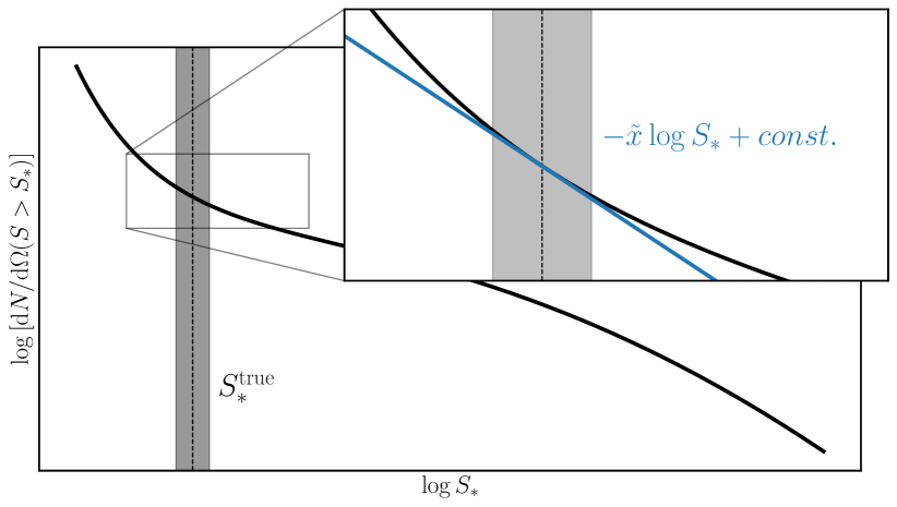
Figure 1: Sketch of the integral number counts (black curve) indicating that the index $\tilde{x}$ is to be measured at the limiting flux $S_{*}$ (dashed line) by fitting a power-law (blue line) in its neighbourhood. Only sources with flux density $S$ in a narrow (shaded) region of fractional width $\mathcal{O}(\beta)$ around $S_{*}$ contribute to the dipole amplitude, so the slope at higher or lower flux density is irrelevant.

We follow the definitions in DB22. In each shell of $r$ we find a distribution of sources with observed spectral flux density $S>S_{*}$,

$$\frac{{\rm d}N}{{\rm d}\Omega{\rm d}r}(r,S>S_{*})=kS_{*}^{-x(r)},$$ (4)

with normalisation $k$, where $x(r)>0$. We then define the normalised distribution

$$f(r)\equiv\frac{{\rm d}N}{{\rm d}\Omega{\rm d}r}(r,S>S_{*})\bigg{/}\int_{0}^{\infty}{\rm d}r\,\frac{{\rm d}N}{{\rm d}\Omega{\rm d}r}(r,S>S_{*}).$$ (5)

(We assume that the integrals converge, either by appropriate choice of $x(r)$ and/or by additionally introducing an appropriate window function $w(r)$.) This distribution is not usually known for a given source sample and requires the knowledge of its luminosity function. In contrast, the flux distribution integrated over comoving distance is an observed quantity

$$\frac{{\rm d}N}{{\rm d}\Omega}(S>S_{*})=\int_{0}^{\infty}{\rm d}r\,\frac{{\rm d}N}{{\rm d}\Omega{\rm d}r}(r,S>S_{*})=k\int_{0}^{\infty}{\rm d}r\,S_{*}^{-x(r)}.$$ (6)

Note that the observed integral source counts need not exhibit perfect power-law behaviour at all thresholds $S_{*}$. In fact, if $x(r)$ is not a constant then a change in slope is inevitable. Consider e.g. $x(r)$ linear in $r$, i.e. $x(r)=x_{0}+x_{1}r$. Eq. (6) then gives

$$\frac{{\rm d}N}{{\rm d}\Omega}(S>S_{*})=\frac{k}{x_{1}\ln S_{*}}S_{*}^{-x_{0}},\quad{\rm for}\,x_{1}\ln S_{*}>0,$$ (7)

where the departure from a pure power-law with index $x_{0}$ is driven by the additional factor $1/\ln S_{*}$. The EB84 test requires the determination of the slope only at the flux density threshold $S_{*}$, as sources with flux densities far from it will not contribute to the dipole amplitude, e.g. a source with very high $S\gg S_{*}$ will remain in the catalogue regardless of the boost applied.

As illustrated in Fig. 1, one should thus measure $\tilde{x}$ locally as the power-law approximation at the flux threshold, i.e.

$$\begin{split}\tilde{x}\equiv&-\frac{{\rm d}}{{\rm d}\ln S_{*}}\left[\ln\frac{{\rm d}N}{{\rm d}\Omega}(S>S_{*})\right]\\ =&-\frac{S_{*}}{\frac{{\rm d}N}{{\rm d}\Omega}(S>S_{*})}\frac{{\rm d}}{{\rm d}S_{*}}\frac{{\rm d}N}{{\rm d}\Omega}(S>S_{*})\\ =&-\frac{S_{*}}{k\int_{0}^{\infty}{\rm d}r\,S_{*}^{-x(r)}}\frac{{\rm d}}{{\rm d}S_{*}}\left[k\int_{0}^{\infty}{\rm d}r\,S_{*}^{-x(r)}\right]\\ =&-\frac{S_{*}}{k\int_{0}^{\infty}{\rm d}r\,S_{*}^{-x(r)}}\left[-k\int_{0}^{\infty}{\rm d}r\,x(r)S_{*}^{-x(r)-1}\right]\\ =&\frac{1}{\int_{0}^{\infty}{\rm d}r\,\frac{{\rm d}N}{{\rm d}\Omega{\rm d}r}(r,S>S_{*})}\int_{0}^{\infty}{\rm d}r\,\frac{{\rm d}N}{{\rm d}\Omega{\rm d}r}(r,S>S_{*})x(r)\\ =&\int{\rm d}r\,f(r)x(r)=x_{\rm eff}.\end{split}$$ (8)

This shows that $x$ measured locally at $S_{*}$ in the observed integral number counts equals the appropriately weighted average as given by $x_{\rm eff}$. E.g. for $x(r)$ linear in $r$ we find $\tilde{x}=x_{\rm eff}=x_{0}+{1/\ln S_{*}}$.

2.2 The spectral index $\alpha$

While DB22 propose an effective value $\alpha_{\rm eff}$ as defined in Eq. (3) we reiterate that the relevant quantity should not be averaged over all sources, but only over those that lie close enough to the threshold $S_{*}$ such that they actually contribute to the dipole amplitude.

Rather than integral source counts we require knowledge of differential source counts that can be evaluated at a given flux density $S$. The integral and differential source counts are related as

$$\frac{{\rm d}N}{{\rm d}\Omega{\rm d}r}(r,S>S_{*})=\int_{S_{*}}^{\infty}{\rm d}S\,\frac{{\rm d}N}{{\rm d}\Omega{\rm d}r{\rm d}S}(r,S).$$ (9)

Using Eq. (4) we find

$$\frac{{\rm d}N}{{\rm d}\Omega{\rm d}r{\rm d}S}(r,S)=kx(r)S^{-x(r)-1},$$ (10)

where we made use, as did DB22, of the fact that $x(r)$ does not depend on $S$. This can be used to define a second distribution function over comoving distance,

$$\begin{split}\tilde{f}(r)\equiv&\left[\frac{{\rm d}N}{{\rm d}\Omega{\rm d}r{\rm d}S}(r,S)\middle/\int_{0}^{\infty}{\rm d}r\,\frac{{\rm d}N}{{\rm d}\Omega{\rm d}r{\rm d}S}(r,S)\right]_{S=S_{*}}\\ =&\,x(r)\frac{{\rm d}N}{{\rm d}\Omega{\rm d}r}(r,S>S_{*})\bigg{/}\int_{0}^{\infty}{\rm d}r\,x(r)\frac{{\rm d}N}{{\rm d}\Omega{\rm d}r}(r,S>S_{*}),\end{split}$$ (11)

where we have used Eqs. (4) and (10). Now $\tilde{\alpha}$ is computed as the average spectral index of sources at the threshold $S_{*}$:

$$\tilde{\alpha}\equiv\int_{0}^{\infty}{\rm d}r\,\tilde{f}(r)\alpha(r),$$ (12)

which is generally different from $\alpha_{\rm eff}$ (3). E.g. for linear $x(r)$ and linear $\alpha(r)=\alpha_{0}+\alpha_{1}r$, we find

$$\tilde{\alpha}=\frac{1}{\tilde{x}}\left(x_{0}\alpha_{0}+\frac{x_{0}\alpha_{1}}{x_{1}\ln S_{*}}+\frac{\alpha_{0}}{\ln S_{*}}+\frac{2\alpha_{1}}{x_{1}(\ln S_{*})^{2}}\right)$$ (13)

to be compared with

$$\alpha_{\rm eff}=\alpha_{0}+\frac{1}{x_{1}\ln S_{*}}\alpha_{1}.$$ (14)

The difference between $\tilde{\alpha}$ and $\alpha_{\rm eff}$ is illustrated by the marginalised distributions shown in Fig. 2: the 2-D distribution ${\rm d}N/{\rm d}S{\rm d}\alpha(S,\alpha)$ returns different 1-D distributions of $\alpha$, if averaged over all $S>S_{*}$, or only in the neighbourhood of $S_{*}$. This highlights the importance of correlations between $S$ and $\alpha$ in a given catalogue; these were in fact accounted for in the mock sky simulations of Secrest et al. (2021). While the area around the flux limit within which sources contribute to the dipole amplitude depends on $\alpha$ (as indicated by the white shaded region in the figure), in practice such corrections are negligible. Lastly, if $x(r)$ is a constant, then $\tilde{\alpha}=\alpha_{\rm eff}$ trivially.

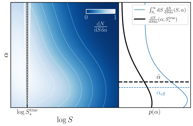
Figure 2: Left panel: Illustrative sketch of the two-dimensional distribution of $S$ and $\alpha$. The spectral index $\tilde{\alpha}$ is to be measured locally at $S_{*}$ (vertical dashed line). As in Fig. 1, only sources with flux density $S$ in a region (grey shaded) close to $S_{*}$ contribute to the dipole amplitude, so the $\alpha$ for other sources are irrelevant. Right panel: Marginalised distributions of $\alpha$ when averaged over all values of $S>S_{*}$ (blue curve) or just over those in the vicinity of $S_{*}$ (black curve) leading to potentially different average values (horizontal dashed lines).

2.3 Dipole amplitude

Using Eqs. (5), (8), (11) and (12), $\tilde{x}$ and $\tilde{\alpha}$ can now be written as

$$\tilde{x}= \!\!\int_{0}^{\infty}\!\!\!{\rm d}r\,\frac{{\rm d}N}{{\rm d}\Omega{\rm d}r}(r,S>S_{*})x(r)\bigg{/}\!\!\!\int_{0}^{\infty}\!\!\!{\rm d}r\,\frac{{\rm d}N}{{\rm d}\Omega{\rm d}r}(r,S>S_{*})$$ (15)

$$\tilde{\alpha}= \!\!\int_{0}^{\infty}\!\!\!{\rm d}r\,\frac{{\rm d}N}{{\rm d}\Omega{\rm d}r}(r,S>S_{*})x(r)\alpha(r)\bigg{/}\!\!\!\int_{0}^{\infty}\!\!\!{\rm d}r\,\frac{{\rm d}N}{{\rm d}\Omega{\rm d}r}(r,S>S_{*})x(r),$$ (16)

using which we now compare Eq. (1) with Eq. (2). Due to the normalisation of $f(r)$ the first terms are trivially equal. The second terms are equal according to Eq. (8). The crucial term therefore is the last:

$$\tilde{x}\tilde{\alpha}= \int_{0}^{\infty}{\rm d}r\,\frac{{\rm d}N}{{\rm d}\Omega{\rm d}r}(r,S>S_{*})x(r)\alpha(r)\bigg{/}\int_{0}^{\infty}{\rm d}r\,\frac{{\rm d}N}{{\rm d}\Omega{\rm d}r}(r,S>S_{*})$$

$$= \int_{0}^{\infty}{\rm d}r\,f(r)x(r)\alpha(r),$$ (17)

since the numerator of Eq. (15) cancels the denominator of Eq. (16). The dipole amplitude then reads

$$\begin{split}\tilde{\mathcal{D}}_{\rm kin}=&\left[2+\tilde{x}(1+\tilde{\alpha})\right]\beta\\ =&\int_{0}^{\infty}{\rm d}r\,f(r)\left[2+x(r)\left(1+\alpha(r)\right)\right]\beta=\mathcal{D}_{\rm kin}.\end{split}$$ (18)

Therefore the dipole amplitude is determined entirely by the observed quantities, $\tilde{x}$ and $\tilde{\alpha}$, which account implicitly for all source evolution effects. Moreover, as shown by DB22, there is exact equivalence between the dipole amplitude computed using the luminosity function (Maartens et al., 2018; Nadolny et al., 2021; Dalang & Bonvin, 2022; Guandalin et al., 2023), and that obtained by taking $x$ and $\alpha$ to be $r$-dependent (Dalang & Bonvin, 2022). Thus we have also demonstrated that the theoretically expected kinematic matter dipole amplitude does not require any knowledge of the luminosity function.

3 Discussion

We have shown that the kinematic matter dipole can be robustly predicted using only observed quantities, as per the EB84 prescription (1), which turned out to be fully equivalent to adding up the contributions (2) from shells of comoving distance. Whereas DB22 highlighted the explicit connection between variations in the intrinsic sample properties $x$ and $\alpha$, and the corresponding computation in a fully general relativistic setting (e.g. Challinor & Lewis, 2011), according to their own calculation (see eq. 36), the equivalence we have shown also implies equivalence with the kinematic matter dipole amplitude calculated using the luminosity function. This makes the determination of the luminosity function redundant in this context, vindicating the assertion of EB84 that “source evolution” is irrelevant in the computation of the kinematic matter dipole.

The difficulty in determining the luminosity function was nevertheless emphasised as a major “theoretical systematic” in predicting the kinematic matter dipole (Guandalin et al. (2023), see also Maartens et al. (2018). This was emphasised by DB22 (see also Dalang & Bonvin, 2023) who questioned the significance of the anomaly found by Secrest et al. (2021) by showing that a range of dipole amplitudes is predicted depending on the choice of the functional form of the magnification bias $x(z)$ and evolution bias $b_{\mathrm{e}}(z)$. Of course this uncertainty only arises due to not knowing the exact functional forms that derive directly from the (unknown) luminosity function of the source sample. However as we have shown, none of this is relevant here. Such uncertainties are entirely bypassed in ensuring to use solely the observed quantities $\tilde{x}$ and $\tilde{\alpha}$ in the EB84 test, as is both appropriate and adequate in the present context. Nevertheless the relation we have found between $\tilde{x}$ and $x(r)$ may prove useful in constraining the magnification bias via measurements of the integral source counts, without reference to the (uncertain) luminosity function as has been done by e.g. Wang et al. (2020).

The correlations first suspected between $x(r)$ and $\alpha(r)$ by DB22 are based on a definition of $\alpha$, namely $\alpha_{\rm eff}$, that does not feature in the EB84 test. These correlations have been investigated empirically by Dam et al. (2023) who invoked the principle of maximal entropy to bound their maximum effect to be below 17% in the quasar sample studied by Secrest et al. (2021). However, we have seen that such correlations need not be studied at all in order to obtain a robust estimate of the dipole amplitude defined in terms of $\tilde{\alpha}$.

Thus no alterations to the EB84 dipole prediction are needed to take into account source evolution effects, as long as the power-law assumptions for the integral source counts and for the source spectra hold at the flux limit $S_{*}$. (This had not been necessary to state explicitly by EB84 who considered perfect power-laws throughout.) Possible curvature in integral source counts ${\rm d}N/{\rm d}\Omega(S>S_{*})$ may warrant small corrections to $\tilde{x}$, as illustrated by the difference between the blue and the black curves in Fig. 1. Also the domain over which to integrate $\alpha$, illustrated by the white shaded area in Fig. 2, offers scope for such corrections. While both are expected to be small corrections to an already small effect of $\mathcal{O}(\beta)$, they can be estimated directly from data. Related corrections were proposed by Tiwari et al. (2014) and implemented by Siewert et al. (2021). While they did not recognise the adequacy of performing the fit of $\tilde{x}$ only locally—e.g.  Siewert et al. (2021) say their fit “extends for each survey over one decade”—they demonstrated the feasibility of the procedure, albeit with little effect on their conclusions.

Lastly, the possible correlation between $\alpha$ and $S$ at the flux limit $S_{*}$ does play a role in the EB84 test, as can be seen by studying $\tilde{\alpha}$ in Fig. 2. This provides justification for the procedure employed by Secrest et al. (2021) to simulate mock skies in order to evaluate the significance with which the dipole measurement rejects the null hypothesis (1). First, $N$ points were distributed randomly on the sky in line with the assumption of isotropy. Each point then was randomly assigned a pair of values $S$ and $\alpha$, sampled from the empirical distribution functions ${\rm d}N/{\rm d}S$ and ${\rm d}N/{\rm d}\alpha$. This respects possible correlations between $S$ and $\alpha$ in the data; in the above context, it amounts to ensuring that in each of the simulations, $\tilde{\alpha}$ is conserved. Later, Secrest et al. (2022) found that the results are nearly unchanged even when $S$ and $\alpha$ are picked independently, which they interpreted as implying that there is no significant source evolution. In light of the present work, we can now confirm that this intuition was correct.

References

- Blake & Wall (2002) Blake C., Wall J., 2002, Nature, 416, 150
- Challinor & Lewis (2011) Challinor A., Lewis A., 2011, Phys. Rev. D, 84, 043516
- Chen & Schwarz (2015) Chen S., Schwarz D. J., 2015, Phys. Rev. D, 91, 043507
- Dalang & Bonvin (2022) Dalang C., Bonvin C., 2022, Mon. Not. Roy. Astron. Soc., 512, 3895
- Dalang & Bonvin (2023) Dalang C., Bonvin C., 2023, Mon. Not. Roy. Astron. Soc., 521, 2225
- Dam et al. (2023) Dam L., Lewis G. F., Brewer B. J., 2023, Mon. Not. Roy. Astron. Soc., 525, 231
- Ellis & Baldwin (1984) Ellis G. F. R., Baldwin J. E., 1984, Mon. Not. Roy. Astron. Soc., 206, 377
- Gibelyou & Huterer (2012) Gibelyou C., Huterer D., 2012, Mon. Not. Roy. Astron. Soc., 427, 1994
- Guandalin et al. (2023) Guandalin C., Piat J., Clarkson C., Maartens R., 2023, Astrophys. J., 953, 144
- Harris et al. (2020) Harris C. R., et al., 2020, Nature, 585, 357
- Hunter (2007) Hunter J. D., 2007, Computing in Science & Engineering, 9, 90
- Laurent et al. (2016) Laurent P., et al., 2016, JCAP, 11, 060
- Maartens et al. (2018) Maartens R., Clarkson C., Chen S., 2018, JCAP, 01, 013
- Milne (1933) Milne E. A., 1933, Z. Astrophys., 6, 1
- Nadolny et al. (2021) Nadolny T., Durrer R., Kunz M., Padmanabhan H., 2021, JCAP, 11, 009
- Peebles & Wilkinson (1968) Peebles P. J. E., Wilkinson D. T., 1968, Phys. Rev., 174, 2168
- Rubart & Schwarz (2013) Rubart M., Schwarz D. J., 2013, Astron. Astrophys., 555, A117
- Secrest et al. (2021) Secrest N. J., von Hausegger S., Rameez M., Mohayaee R., Sarkar S., Colin J., 2021, Astrophys. J. Lett., 908, L51
- Secrest et al. (2022) Secrest N. J., von Hausegger S., Rameez M., Mohayaee R., Sarkar S., 2022, Astrophys. J. Lett., 937, L31
- Siewert et al. (2021) Siewert T. M., Schmidt-Rubart M., Schwarz D. J., 2021, Astron. Astrophys., 653, A9
- Singal (2011) Singal A. K., 2011, Astrophys. J. Lett., 742, L23
- Stewart & Sciama (1967) Stewart J. M., Sciama D. W., 1967, Nature, 216, 748
- Tiwari et al. (2014) Tiwari P., Kothari R., Naskar A., Nadkarni-Ghosh S., Jain P., 2014, Astropart. Phys., 61, 1
- Virtanen et al. (2020) Virtanen P., et al., 2020, Nature Methods, 17, 261
- Wang et al. (2020) Wang M. S., Beutler F., Bacon D., 2020, Mon. Not. Roy. Astron. Soc., 499, 2598
- Watkins et al. (2023) Watkins R., et al., 2023, Mon. Not. Roy. Astron. Soc., 524, 1885