A Bayesian Estimator of Sample Size

Abstract

We consider a Bayesian estimator of sample size (BESS) and an application to oncology dose optimization clinical trials. BESS is built upon three pillars, Sample size, Evidence from observed data, and Confidence in posterior inference. It uses a simple logic of “given the evidence from data, a specific sample size can achieve a degree of confidence in the posterior inference.” The key distinction between BESS and standard sample size estimation (SSE) is that SSE, typically based on Frequentist inference, specifies the true parameters values in its calculation while BESS assumes possible outcome from the observed data. As a result, the calibration of the sample size is not based on type I or type II error rates, but on posterior probabilities. We demonstrate that BESS leads to a more interpretable statement for investigators, and can easily accommodates prior information as well as sample size re-estimation. We explore its performance in comparison to the standard SSE and demonstrate its usage through a case study of oncology optimization trial. BESS can be applied to general hypothesis tests. An R tool is available at https://ccte.uchicago.edu/BESS.

Clinical Trial; Confidence; Evidence; Hypothesis testing; Posterior inference; Priors; Type I error.

1 Introduction

1.1 Motivation

In drug development, the clinical objective is to establish the drug’s effectiveness and safety. Randomized clinical trials (RCTs) are the gold standard to achieve the objective. As it is usually impractical to include all patients from a disease population, RCTs take a random sample of certain size to address the clinical question through statistical inference. Due to the law of large numbers, the larger the sample size, the more precise the estimated treatment effect is but also the more costly the trial is. Therefore, in practice a sample size estimation (SSE) is usually conducted before the trial starts to balance the tradeoff between precision in statistical inference and trial cost.

We consider a Bayesian framework for SSE. The research is motivated by the recent change in early-phase oncology drug development that recommends randomized comparison of multiple doses. In the past two decades, oncology drug development has benefited from biological and genomics breakthroughs and novel cancer drugs are no longer based on cytotoxic one-size-fits-all mechanism like chemicals or radiations. Instead, targeted, immune, and gene and cell therapies combat tumor cells by precisely altering oncogenic cellular or molecular pathways. Consequently, the traditional monotonic dose-response relationship is no longer valid for many novel cancer drugs. Instead, efficacy often plateaus or even decreases after dose rises above certain level. To this end, US FDA launched Project Optimus (Food et al., 2023; Shah et al., 2021; Blumenthal et al., 2021) aiming to transform the early-phase oncology drug development. The main objective of the project is to identify an optimal dose, potentially lower than the maximum tolerated dose but with at least comparable anti-tumor effect. The new dose optimization paradigm recommends a randomized comparison of two or more doses following an initial dose escalation. While randomized trial design and SSE are routinely conducted in drug clinical trials, they are new in dose-optimization trials, usually restricted by limited resources. Type I/II error rates for standard SSE are rarely the main objective for early-phase of drug development. Instead, investigators are more concerned about the accuracy in the trial decision making, such as selecting the right dose or starting confirmatory studies, which may be very costly. Current SSE for dose optimization trials is often based on ad-hoc choices, such as using a small sample size of 20 patients per dose. This leads to a question of how much is expected to learn from the 20 patients, or whatever the number may be. Moreover, clinical trials that use human subjects for clinical research should always provide a reasonable justification for the number of subjects to be enrolled. We attempt to fill the gap by considering a Bayesian approach for sample size estimation.

1.2 Review of SSE Methods

In the literature, standard SSE methods (Adcock, 1997; Wittes, 2002; Desu, 2012) are based on Frequentist hypothesis testing by controlling the type I error rate $\alpha$ to achieve a desirable power $(1-\beta)$, assuming the true population parameters are known. For example, a sample size statement for a two-arm RCT based on binary outcome is as follows:

• Statement 1: At type I error rate of $\alpha$, with a clinically minimum effect size $\theta^{*}$, $S$ subjects are needed to achieve $(1-\beta)$ power when the response rates for the treatment and control arms are $\theta_{1}$ and $\theta_{0}$.

A comprehensive review can be found in Wang and Ji (2020). In addition, sample size may be determined based on hybrid Frequentist-Bayesian inference as in Ciarleglio and Arendt (2017); Berry et al. (2010). These methods use Bayesian models but calibrate sample size based on type I error rate and power via simulation. In contrast, some methods use Bayesian properties for sample size estimation such as the length, coverage of posterior credible intervals, Bayes factors under sampling and fitting priors (Lin et al., 2022), or loss functions like $k\cdot\text{False Positive Rate}+\text{False Negative Rate}$ (Müller et al., 2004).

Several methods attempt to bridge the SSE philosophies between Frequentist and Bayesian methods. Notable contributions include Kunzmann et al. (2021), Inoue et al. (2005), and Lee and Zelen (2000). In particular, Lee and Zelen (2000) propose to link posterior estimates with type I/II error rates, and estimate sample size by providing posterior probabilities rather than the Frequentist error rates. The authors advocate defining “statistical significance” as the trial outcome having a large posterior probability of being correct. However, their sample size calculation still follows standard SSE approach.

1.3 Main idea

To this end, we propose a new Bayesian estimator of sample size (BESS) based on a general hierarchical modeling framework and posterior inference. Let $\bm{y}$ denote the observed data and $\bm{\theta}$ the unknown parameters as generic notation. We assume a Bayesian hierarchical model is to be used for the experimental design and data analysis. Our main idea is originated from noticing a simple trend between the sample size and observed effect size from data. Suppose in a two-arm RCT with sample size $n$ per arm and a binary outcome, we are interested in testing if the effect size (difference in response rates), defined as $\theta=(\theta_{1}-\theta_{0})$ between the treatment (1) and control (0) is greater than a clinically minimum effect size $\theta^{*}$. This can be formulated as testing the null hypothesis $H_{0}:\theta\leq\theta^{*}$ versus the alternative $H_{1}:\theta>\theta^{*}.$ Suppose after the trial is completed, the observed response rates are $\bar{y}_{1}$ and $\bar{y}_{0}$ for the treatment and control arms, respectively. A Frequentist $z$-test is used to test the hypotheses given by

$$z^{*}=\frac{(\bar{y}_{1}-\bar{y}_{0})-\theta^{*}}{\sqrt{[\bar{y}_{1}(1-\bar{y}_{1})+\bar{y}_{0}(1-\bar{y}_{0})]/n}.}$$

If we assume, for the sake of argument, that $\bar{y}_{1}=0.3$, we find in the table below the relationship between the sample size $n$ and $(\bar{y}_{1}-\bar{y}_{0})$, for reaching the same $z^{*}$ value of 1.64, i.e., a one-sided $p$-value of 0.05. We call $(\bar{y}_{1}-\bar{y}_{0})$ the “evidence.” In order to reach the same Frequentist statistical significance, sample size needs to increase in order to achieve $z^{*}=1.64\,(p\mbox{-value}=0.05)$ when evidence decreases.

Sample size ($n$)	10	20	30	50	100	500	1000
Evidence ($\bar{y}_{1}-\bar{y}_{0}$)	0.29	0.24	0.21	0.18	0.15	0.10	0.08
$z^{*}\,(p\mbox{-value})$	1.64 (0.05)

Instead of using a Frequentist inference like the $z$-test, we consider Bayesian hypothesis testing based on posterior probability of the alternative hypothesis, which, in the setting of clinical trials, refers to the success of the trial. Decision of accepting the alternative hypothesis is by thresholding the posterior probability of $H_{1}$ at a relatively large value $c\in(0,1)$. Assume a Bayesian hierarchical model is given by $f(\bm{y}\mid\bm{\theta})\pi(\bm{\theta}\mid H)\pi(H)$, where $H=H_{0}$ or $H_{1}$ is a binary indicator of the null and alternative hypotheses. The proposed BESS aims to find a balance between 1) “Sample size” $S$ of the clinical trial, 2) “Evidence” defined as the observed treatment effect $e=(\bar{y}_{1}-\bar{y}_{0})$, and 3) “Confidence” defined as the posterior probability of the alternative hypothesis.

Consider the previous example of testing if the treatment effect $\theta=(\theta_{1}-\theta_{0})$ is greater than $\theta^{*}$, a minimum effect size. BESS provides a sample size statement as follows:

• Statement 2: Assuming the evidence is at least $e$, $S$ subjects are needed to declare with confidence $c$ that the treatment effect is at least $\theta^{*}$.

Note that “evidence” is a function of the data, not parameters, and “confidence” refers to $\text{Pr}(H_{1}|\bm{y})$, the posterior probability of the alternative hypothesis, i.e., the treatment effect is at least $\theta^{*}.$ Comparing Statement 1 and Statement 2, one can see that the two statements are based on different statistical properties, Frequentist type I/II error rates for Statement 1 and Bayesian posterior probabilities for Statement 2. Also, while Statement 1 assumes the true values of the parameters are given, Statement 2 assumes what might be observed from the trial data. We will show that the BESS and associated Statement 2 is easier to interpret in practice since it directly addresses the uncertainty in the decision to be made for the trial at hand, measured by posterior probabilities.

The remainder of the article is organized as follows: Section 2 presents the proposed probability model. Section 3 describes the BESS method. Section 4 illustrates some of the proprieties of BESS, including the relationships among sample size, evidence, and confidence, as well as the coherence between BESS and Bayesian inference. Section 5 reports the operating characteristics of BESS with comparison to the standard SSE method. Section 6 illustrates the applications of BESS to a hypothetical dose optimization trial. Finally, we conclude the article in Section 7.

2 Probability Model

We consider BESS for both one-arm and two-arm trials. Denote $y_{ij}$ the outcome of patient $i$ in arm $j$, where $i=1,\ldots,n,$ index the patients, and $j=0$ and $1$ index the control and treatment arm, respectively. When needed, we drop index $j$ and use $y_{i}$ for one-arm trials. Let $\theta_{1}$ denote the true response parameter for the treatment arm, and let $\theta_{0}$ be the true response parameter for the control arm in a two-arm trial or the reference response parameter in a one-arm trial. Let $\theta=f(\theta_{0},\theta_{1})$ a function of $\theta_{0}$ and $\theta_{1}$ denote the treatment effect. For example, we consider $\theta=(\theta_{1}-\theta_{0})$ in this paper although its form can be generalized. Consider hypotheses

$$H_{0}:\theta\leq\theta^{*}\text{ vs. }H_{1}:\theta>\theta^{*},$$ (1)

where $\theta^{*}$ is a minimum size for treatment effect deemed clinically relevant. Let $H$ be the binary random variable taking $H_{0}$ or $H_{1}$ with probability $(1-q)$ and $q$, respectively.

We propose a Bayesian hierarchical model for testing the hypotheses (1). Let

$$y_{ij}|\theta_{j} \sim f(\theta_{j}),$$

$$(\theta_{0},\theta_{1})|\tilde{\bm{\theta}},H=H_{j} \sim \pi(\theta_{0},\theta_{1}|\tilde{\bm{\theta}})I(\theta\in H_{j}),$$ (2)

$$\text{Pr}(H=H_{1}) = q,$$

where $f(.)$ represents the likelihood function, $\pi(\theta_{0},\theta_{1}|\tilde{\bm{\theta}})$ is a joint prior distribution for $(\theta_{0},\theta_{1})$, $\tilde{\bm{\theta}}$ are hyper-parameters, and $I(x\in A)$ is the indicator function which equals 1 if $x\in A$ and 0 otherwise. For simplicity, we consider $\pi(\theta_{0},\theta_{1}|\tilde{\bm{\theta}})=\pi_{0}(\theta_{0}|\tilde{\bm{\theta}})\pi_{1}(\theta_{0}|\tilde{\bm{\theta}})$, where $\pi_{0}=\pi_{1}$.

In this work, we consider three specific types of outcome $y_{ij}$: binary, continuous, and count. A summary of the parameter $\theta_{j}$, likelihood function $f(.)$, and prior distribution $\pi_{j}$ for $\theta_{j}$ is shown in Table 1. We consider conjugate prior for simplicity and computational convenience although the proposed BESS works for any general priors. While it is not the focus of this work to discuss choice of priors, we note the flexibility of BESS to incorporate various priors in real-life applications. For example, when little prior information is known vague priors like Jeffrey’s prior may be considered; in contrast, it is also possible to use informative priors when prior information is available. For instance, assume a previous trial with binary outcome has completed with a sample size of $n_{0}$ patients of whom their outcome data are available, denoted as $\bm{y}^{0}=\{y_{i}^{0};i=1,\ldots,n_{0}\}$. Then, one could consider an informative prior $\pi_{1}(\theta_{1})=\text{Beta}(a,b)$ and set $a=a^{*}+\sum_{i=1}^{n_{0}}y_{i}^{0},\,\,b=b^{*}+n_{0}-\sum_{i=1}^{n_{0}}y_{i}^{0},$ where $a^{*}$ and $b^{*}$ are small (e.g., $a^{*}=b^{*}=0.5$).

Table 1: Summary of parameter, likelihood function, and prior distribution for different outcome types.

Outcome type	Parameter $\theta_{j}$	Likelihood $f(\cdot)$	Prior distribution $\pi_{j}(\tilde{\bm{\theta}})$
Binary	Response rate	$\text{Bern}(\theta_{j})$	$\text{Beta}(a,b)$
Continuous	Mean response	$N(\theta_{j},\sigma^{2})$, $\sigma$ known	$N(a,b)$
Count-data	Event rate	$\text{Poi}(\theta_{j})$	$\text{Gamma}(a,b)$

3 Confidence, Evidence, and Sample Size

3.1 Confidence

We introduce the three pillars of BESS, Confidence, Evidence, and Sample Size. We start with “Confidence”, the confidence of posterior inference, expressed mathematically as the posterior probability of the alternative hypothesis $\text{Pr}(H=H_{1}|\bm{y}_{n}),$ where $\bm{y}_{n}$ denotes the data with sample size $n$. The optimal decision rule under a variety of loss functions (Müller et al., 2004) is to reject the null $H_{0}$ and accept $H_{1}$ if $\text{Pr}(H=H_{1}|\bm{y}_{n})\geq c$ for a high value of $c\in(0,1).$ The higher $c$ is, the more confident is the decision. To see this, one simply observes that $(1-c)$ is the upper bound of posterior probability of a wrong rejection since when $H_{0}$ is rejected, $\text{Pr}(H=H_{0}|\bm{y}_{n})<c$.

According to model (2), it is straightforward to show that

$$\text{Pr}(H=H_{1}|\bm{y}_{n})=\frac{q\cdot\int_{\bm{\theta}\in H_{1}}f(\bm{\theta}|\bm{y}_{n})d\bm{\theta}}{1-q+[(2q-1)\cdot\int_{\bm{\theta}\in H_{1}}f(\bm{\theta}|\bm{y}_{n})d\bm{\theta}]}.$$ (3)

If we assume a priori, both hypotheses are equally likely, i.e., $q=0.5$, then equation (3) may be further reduced to

$$\text{Pr}(H=H_{1}|\bm{y}_{n})=\int_{\bm{\theta}\in H_{1}}f(\bm{\theta}|\bm{y}_{n})d\bm{\theta}.$$ (4)

If conjugate priors in Table 1 are used, $f(\theta_{j}|\bm{y}_{jn})$ have closed-form solutions. Otherwise, numerical evaluation of (3) or (4) is needed.

3.2 Evidence

Evidence is the main metric that differentiates BESS from a standard SSE. In short, we define evidence as a function of data, $e(\bm{y}_{n})$, that reflects the strength of treatment effect. In the settings listed in Table 1 we consider evidence defined as

$$e=\bar{y}-\theta_{0}\text{ for one-arm trials, and }e=\bar{y}_{1}-\bar{y}_{0}\text{ for two-arm trials}.$$ (5)

In simple words, evidence $e$ is the observed effect size from the trial data before they are observed. This means that in order to apply BESS, investigator needs to pre-specify (and calibrate) the potential observed effect size before the trial is conducted. This is analogous to the requirement of specifying the true parameter values in the standard SSE, except BESS assumes what might be observed rather than what might be true. We consider evidence $e$ as a function of the sufficient statistic in Table 1. For the three outcomes in one-arm trials, $(e+\theta_{0})$ is exactly the sufficient statistic. For two-arm trials, $e$ is the difference between the sufficient statistics $(\bar{y}_{0},\bar{y}_{1})$ of the two arms. Being a function of sufficient statistics allows for a search algorithm to find an appropriate sample size under BESS, which will be clear next.

3.3 Sample Size of BESS

We first briefly review the standard SSE based on Frequentist inference. Considering a $z$-test for a two-arm trial with binary outcome, the standard sample size approach assumes true values of $\theta_{1}$ and $\theta_{0}$, and solves for $n$ based on desirable type I/II error rates $\alpha$/$\beta$ given by

$$n=\frac{(z_{\alpha}+z_{\beta})^{2}}{(\theta-\theta^{*})^{2}}[\theta_{1}(1-\theta_{1})+\theta_{0}(1-\theta_{0})].$$ (6)

In BESS, we find the sample size through a similar argument but using posterior inference instead. Investigators specify the confidence $c$, so that

$$\text{Pr}(H=H_{1}|\bm{y}_{n})\geq c,$$ (7)

where $\text{Pr}(H=H_{1}|\bm{y}_{n})$ is computed by equation (3). In Müller et al. (2004) decision rule (7) is shown to be optimal for a variety of common loss functions, such as the posterior expected loss of $k\cdot\text{FPR}+\text{FNR}$, where FPR and FNR are false positive and negative rates, respectively. Next, we provide three algorithms for sample size calculation based on BESS and models in Table 1.

One-arm trial

For one-arm trials, with the settings of likelihood and prior in Table 1, we can show that $\text{Pr}(H=H_{1}|\bm{y}_{n})=\text{Pr}(H=H_{1}|e,n).$ See Appendix A.1 for detail. Therefore, by fixing $e$ and $c$, we can find the smallest sample size $n$ that satisfies (7). This leads to the proposed BESS Algorithm 1 and the corresponding sample size statement BESS 1.

BESS 1: Assuming the evidence is $e$, $n$ subjects are needed to declare with confidence $c$ that the treatment effect is larger than $\theta^{*}$.

Two-arm trial; Continuous data, known variance

Second, for two-arm trials and continuous outcome with normal likelihood and known variance, we still have $\text{Pr}(H=H_{1}|\bm{y}_{n})=\text{Pr}(H=H_{1}|e,n).$ See Appendix A.2 for detail. Therefore, BESS Algorithm 1 applies. And we have the sample size statement BESS 2.1.

BESS 2.1: Assuming the evidence is $e$ and variance $\sigma^{2}$ is known for each arm, $n$ subjects per arm are needed to declare with confidence $c$ that the treatment effect is larger than $\theta^{*}$.

BESS Algorithm 1 below provides steps for finding $n$ in BESS 1 and BESS 2.1.

BESS Algorithm 1 One-arm trials; two-arm trials with continuous data and known variance

1:Input: The hierarchical models in Table 1.

2:Input: Clinically meaningful effect size $\theta^{*}$, evidence $e$, confidence $c$, prior probability $q$, reference response rate $\theta_{0}$ (for one-arm trials).

3:Set $n_{\text{min}}$ and $n_{\text{max}}$ ($n_{\text{min}}<n_{\text{max}}$) the smallest and largest candidate sample sizes.

4:Set $n=n_{\text{min}}.$

5:while $n\leq n_{\text{max}}$ do

6:     Compute equation (3).

7:     if condition (7) is true then

8:         Stop and return the sample size $n$.

9:     else

10:         $n=n+1$

11:     end if

12:end while

13:if $n>n_{\text{max}}$ then

14:     Return sample size is larger than $n_{\text{max}}.$

15:end if

Two-arm trial; Binary and Count data

For binary and count data in two-arm trials, $\text{Pr}(H=H_{1}|\bm{y}_{n})=\text{Pr}(H=H_{1}|\bar{y}_{1},\bar{y}_{0},n)$. See Appendix A.3 for a quick proof. Since $e=(\bar{y}_{1}-\bar{y}_{0})$, fixing evidence $e$ does not uniquely define $\text{Pr}(H=H_{1}|\bm{y}_{n}).$ Hence, we propose to specify evidence $e$ and find all pairs of $\bar{y}_{1}$ and $\bar{y}_{0}$ that satisfies $e=(\bar{y}_{1}-\bar{y}_{0})$. We then find the minimum posterior probability of $H_{1}$ among these pairs of $\bar{y}_{1}$ and $\bar{y}_{0}$, i.e.,

$$\text{Pr}(H=H_{1}|e,n)=\min_{\bar{y}_{1},\bar{y}_{0}}\{\text{Pr}(H=H_{1}|(\bar{y}_{1},\bar{y}_{0},n));\forall\bar{y}_{1}-\bar{y}_{0}=e\}.$$ (8)

Then the sample size statement for a two-arm trial is the same as BESS 1. And BESS Algorithm 2 provides details of finding the sample size $n$ for a two-arm trial.

BESS Algorithm 2 Two-Arm Trials; Binary or Count Data

1:Input: The hierarchical models in Table 1.

2:Input: Clinically meaningful effect size $\theta^{*}$, evidence $e$, confidence $c$, prior probability $q$.

3:Set $n_{\text{min}}$ and $n_{\text{max}}$ ($n_{\text{min}}<n_{\text{max}}$) the smallest and largest candidate sample sizes.

4:Set $n=n_{\text{min}}$.

5:while $n\leq n_{\text{max}}$ do

6:     Find all pairs of $(\bar{y}_{1},\bar{y}_{0})$ where $\bar{y}_{1}-\bar{y}_{0}=e$.

7:     for each pair of $(\bar{y}_{1},\bar{y}_{0})$ do

8:         Compute equation (3).

9:     end for

10:     Compute equation (8).

11:     if $\text{Pr}(H=H_{1}|e,n)\geq c$ then

12:         Stop and return the sample size $n$.

13:     else

14:         $n=n+1$.

15:     end if

16:end while

17:if $n>n_{\text{max}}$ then

18:     Return sample size is larger than $n_{\text{max}}$.

19:end if

Alternatively, one may wish to specify the values of $\bar{y}_{1}$ and $\bar{y}_{0}$ directly instead of their difference $e$. Since $(\bar{y}_{1},\bar{y}_{0})$ is sufficient, the sample size search algorithm becomes easier. To this end, we propose a simple variation BESS Algorithm 2’ in Appendix A.4 and statement BESS 2.2 assuming $(\bar{y}_{1},\bar{y}_{0})$ are given.

BESS 2.2 Assuming the response parameters in treatment and control arms are $\bar{y}_{1}$ and $\bar{y}_{0}$, respectively, $n$ subjects per arm are needed to declare with confidence $c$ that the treatment effect is larger than $\theta^{*}$.

Discrete Data

Lastly, since binary and count data are integer-valued, not all specified evidence value $e$ can be achieved for a given sample size in the proposed BESS Algorithms 1 and 2. For example, when the outcome is binary and sample size $n=10$, it is impossible to observe evidence $e=0.15$ since this requires having $n\cdot e=1.5$ more responders in the treatment arm than the control. The number of responders cannot be a fraction. To this end, we propose to round down the specified $e$ to the nearest possible value for a given $n$ by $e^{\prime}=\frac{1}{n}\lfloor n\cdot e\rfloor,$ where $\lfloor.\rfloor$ is the floor function. This gives a conservative estimate of the sample size since even with smaller evidence, the sample size would still ensure the needed confidence.

4 Properties of BESS

4.1 Correlation between sample size, evidence, and confidence

We explore the relationship of the three pillars of BESS, sample size, evidence, or confidence. Specifically, we fix one and report the correlation of the remaining two using a two-arm trial with binary outcome. Similar results can be achieved for other types of data or one-arm trials.

Positive correlation between confidence and evidence, Figure 1(a)

We compute confidence using equation (3) for various values of evidence $e$, while keeping the sample size $n$ constant. Figure 1(a) presents a line plot of the posterior probability of $H_{1}$ (the confidence) against various values of evidence, when sample size is set at $n=10,$ $20,$ or $30$, assuming $\theta^{*}=0.05$. This plot demonstrates that confidence increases monotonically from 0 to 1 as evidence shifts from -1 to 1. When evidence is negative, the data does not support the alternative hypothesis and therefore the confidence (that the alternative is true) drops to zero. When evidence is positive, the confidence improves. Interestingly, the order of confidence across different sample sizes flips when evidence is near 0, giving smaller sample size more confidence. This is expected since when evidence is small, a larger sample size should imply less confidence of the alternative hypothesis.

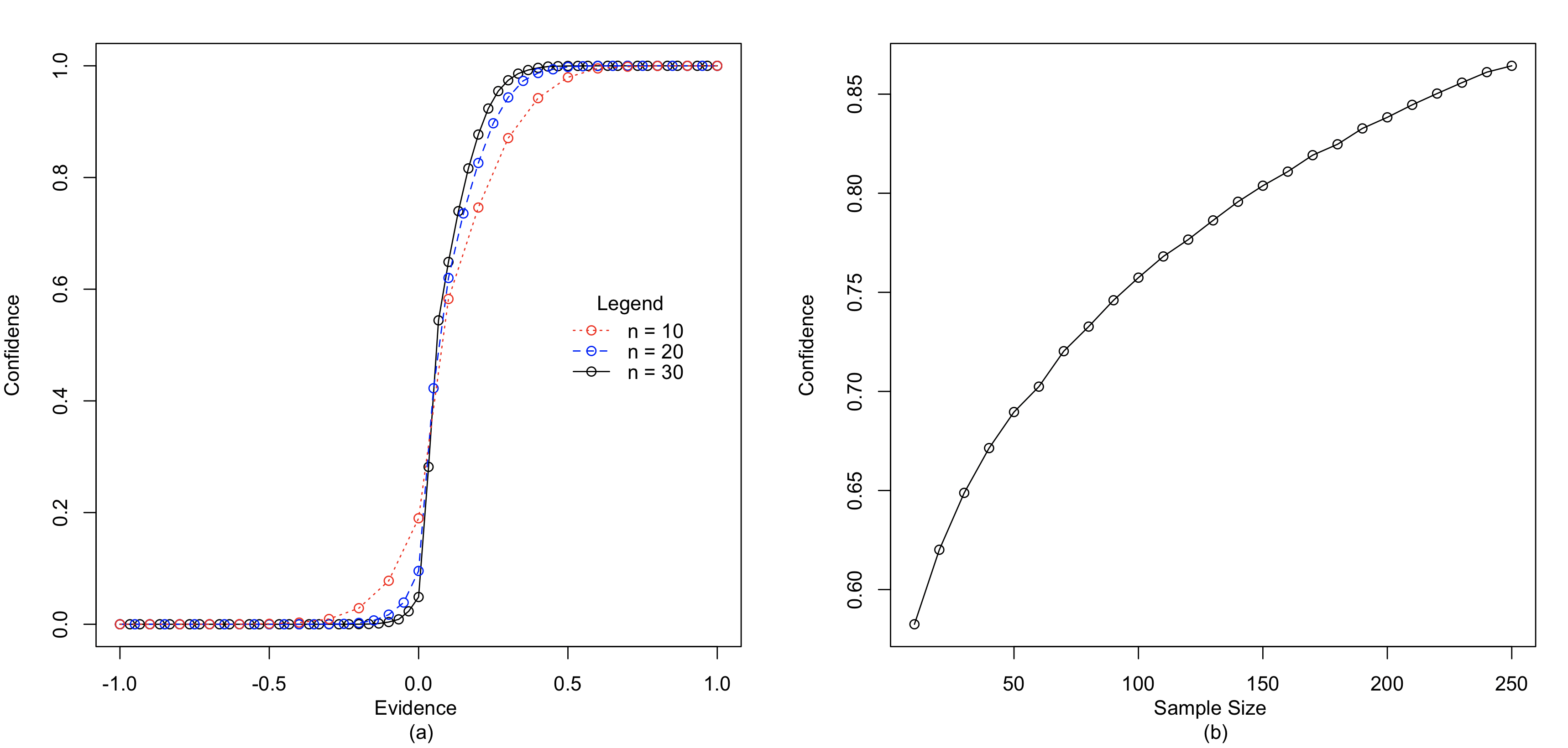
Figure 1: The line plots of (left) confidence vs. evidence when sample size is fixed to be $n=10,20,\text{ and }30$, and (right) confidence vs. sample size when $e=0.1$. The result assumes binary outcome for two-arm trial, with $\theta^{*}=0.05$.

Positive correlation between sample size and confidence, Figure 1(b)

We again compute confidence using equation (3), varying the sample size $n$ while keeping the evidence $e$ constant. Figure 1(b) demonstrates the positive relationship between sample size and confidence, when $e=0.1$ and $\theta^{*}=0.05$. This is expected when evidence is supportive of the alternative hypothesis since the larger the sample size , the larger the posterior probability of $H_{1}$.

Negative correlation between evidence and sample size

We next explore the correlation between evidence and sample size, maintaining a fixed confidence level at $\text{Pr}(H=H_{1}|e,n)=0.6.$ For this demonstration, we calculate confidence using (3) across a range of evidence and sample sizes. For example, with $n=10$ patients per arm, the potential range of evidence $e$ - reflecting the difference in percent responders between the treatment and control arms - spans from -1 to 1, with increments of 0.1.

Given the discrete nature of the outcomes, it’s not always possible to find an evidence level for each sample size $n$ that exactly matches $\text{Pr}(H=H_{1}|e,n)=0.6$. Thus, we document the smallest $e$ for each $n$ where $\text{Pr}(H=H_{1}|e,n)\geq 0.6$. In this case, for $\theta^{*}=0.05$, we report $n(e)$, the different sample sizes $n$ with their corresponding evidence $e$: $50(0.080)$, $100(0.070)$, $150(0.067)$, $200(0.065)$, and $1000(0.057)$. These values clearly show that as sample size increases, evidence needed to maintain the confidence at 0.6 decreases, approaching $\theta^{*}=0.05$.

4.2 Coherence between BESS and Bayesian Inference

In the proposed BESS approach, the evidence $e(\bm{y}_{n})$ is a function of the trial data $\bm{y}_{n}$. In addition, the confidence, defined as the posterior probability $\text{Pr}(H_{1}|\bm{y}_{n}),$ is also a function of $\bm{y}_{n}$. Let’s take a look at the BESS sample size statement again. It can be generalized as

For assumed evidence $e$, a sample size of $n$ will provide confidence $c$ that the alternative hypothesis is true.

After the trial is conducted and data observed, a Bayesian analysis of the observed data using posterior probability will be coherent with the BESS statement. To explain this, we first denote $\bm{y}^{\star}_{n}$ the observed data after the trial is completed, $e^{\star}$ the observed evidence, and $c^{\star}=\text{Pr}(H_{1}|\bm{y}^{\star}_{n})$ the posterior probability of $H_{1}$ conditional on the observed data $\bm{y}^{\star}_{n}.$ Then the coherence between BESS and Bayesian inference means:

If $e^{\star}>e$, then $c^{\star}>c.$

Coherence is important for BESS to be adopted in practice since investigators of clinical trials are usually not statisticians, and the coherence property of BESS allows them to connect the design (i.e., sample size statement) of the trial with the statistical analysis of the observed data once the trial is carried out.

To verify the coherence property numerically, we perform a simple simulation. In Appendix Table A.1 we set up the true parameters for data simulation for each type of clinical trial data. For example, for two-arm binary data, we assume the minimum treatment effect $\theta^{*}=0.05$, evidence $e=0.1$, confidence $c=0.8$. Using a prior distribution $\theta_{j}\sim\text{Beta}(0.5,0.5)$ BESS leads to a sample size of 150. We then repeatedly generate trial data assuming different true values of $\theta_{1}$ and $\theta_{0}$ in Table A.1, and report the inference results of $e^{\star}$ and $c^{\star}$. Figure 2 summarizes the simulation results. In all three subplots (a)-(c), when $e^{\star}$ is larger than $e$ represented by the black vertical line, $c^{\star}$ is larger than $c$, the red horizontal line.

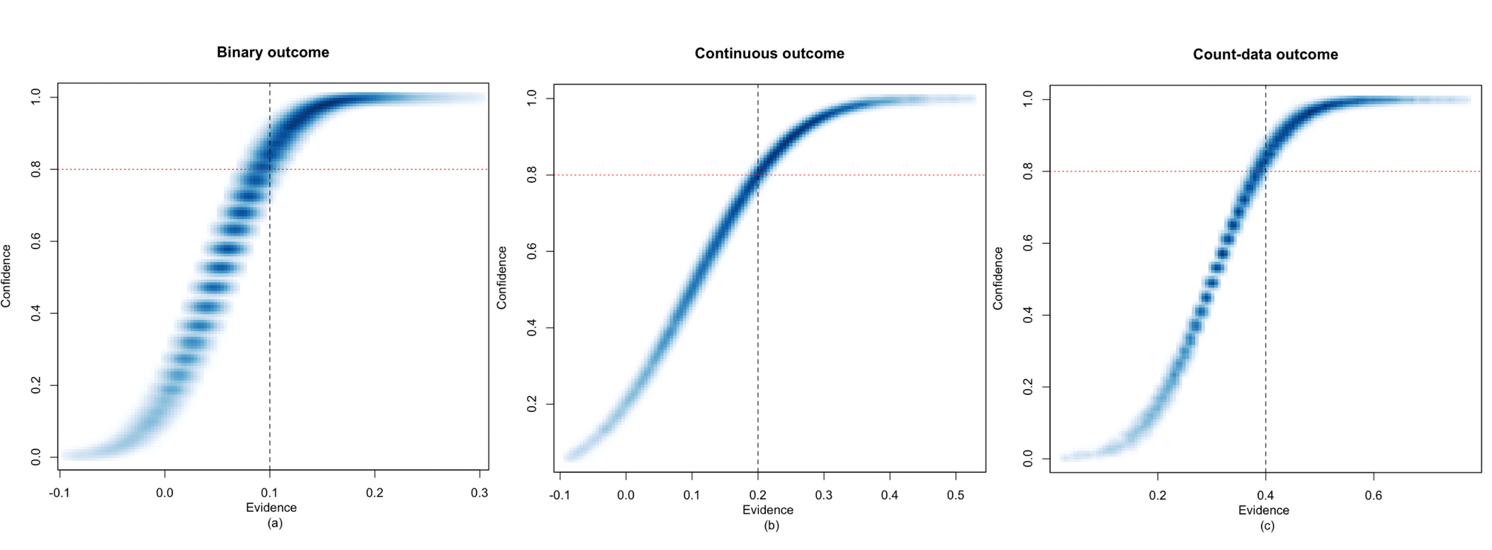
Figure 2: Plots of observed confidence $c^{\star}$ vs. observed evidence $e^{\star}$ for binary, continuous, and count-data outcomes with two-arm trial. The black vertical dashed line shows the location of $e^{\star}=e$, and the red horizontal dotted line shows the location of $c^{\star}=c$.

5 Comparison with Standard SSE

5.1 Simulation Setup

Through simulation, we compare BESS and the standard SSE for a two-arm trial with binary outcome. For fair comparison, we match the type I/II error rates for both methods. The matching is realized by three steps. Step 1: we obtain sample size estimated via the proposed BESS approach for a trial. Step 2: we repeatedly simulate trial data under the null and alternative hypotheses, perform the Bayesian inference using the same model as in BESS, and record the type I and type II error rates from the simulated trials. Step 3: using the two error rates, we apply the standard SSE to arrive at a Frequentist sample size, and compare it with the BESS estimate. See Appendix Figure A.1 for an illustration.

Step 1: BESS sample size

We consider a two-arm trial with binary outcome and let $\theta_{1}$ and $\theta_{0}$ be the response rates, and $\theta^{*}$ the clinical minimum effect size. The trial aims to test $H_{0}:\theta_{1}-\theta_{0}\leq\theta^{*}\text{ vs. }H_{1}:\theta_{1}-\theta_{0}>\theta^{*}.$ For BESS, we assume a binomial likelihood, an improper prior $(\theta_{1},\theta_{0})|H_{j}\sim\text{Beta}(0,0)\cdot\text{Beta}(0,0)I((\theta_{1},\theta_{0})\in H_{j})$, and $\text{Pr}(H=H_{1})\equiv q=0.5.$ We apply BESS Algorithm 2 to obtain a sample size for a pair of desirable evidence $e$ and confidence cutoff $c$. We try several different pairs of $e$ and $c$ as well, listed in Table 2.

Step 2: Estimate type I/II error rates

Next, for each BESS sample size in Step 1, we repeatedly simulate trials under the null $H_{0}$ and the alternative $H_{1}$ to numerically compute the type I/II error rates. Specifically, under the null we let $\theta_{1}=0.3$ and $\theta_{0}=0.25$, and under the alternative, $\theta_{1}=0.4$ and $\theta_{0}=0.25$. We set $\theta^{*}=0.05.$

Based on each pair of $\theta_{1}$ and $\theta_{0}$ values, we generate the binary responses of 150 patients per arm for the treatment arm and control arm. Denote the simulated outcomes $\bm{y}_{n}=\{\bm{y}_{n1}\text{ and }\bm{y}_{n0}\}$, $\bm{y}_{nj}=\{y_{ij};i=1,\ldots,n\},\,j=0,1.$ We generate $y_{ij}\sim\text{Bern}(\theta_{j})$ where $\text{Bern}(\theta)$ is a Bernoulli distribution with mean $\theta.$ The null is rejected if $\text{Pr}(H=H_{1}|\bm{y}_{n})>0.8.$ Here, $0.8$ is arbitrarily selected without specific intention. A larger or smaller cutoff than $0.8$ arbitrarily affects the computed type I/II error rates, which does not affect the objective of our simulation. We simulate 10,000 trials each under the null and alternative. A rejection of the null for a trial simulated under the null is recorded as an incidence of type I error and a non-rejection of the null for a trial under the alternative is recorded as an incidence of type II error. The type I/II error rates $(\alpha/\beta)$ are then computed as the frequencies of the corresponding incidences over the 10,000 trials.

Step 3: Estimate Frequentist sample size and compare with BESS

Based on the computed type I/II error rates $(\alpha/\beta)$ from Step 2, denoted as $\alpha$ and $\beta$, we estimate a sample size using a standard SSE approach. For example, we consider a superiority $z$-test for comparing $\theta_{1}$ and $\theta_{0}$, and a sample size can be estiamted via (6). In the estimation, we assume the true values for $\theta_{1}$ and $\theta_{0}$ under the alternative, which gives the standard approach an “oracle” performance. In other words, the estimated sample size is guaranteed to achieve the target Type I/II error rates $\alpha$ and $\beta$, since the assumed $\theta_{1}$ and $\theta_{0}$ in the sample size estimation match the true values. Even though this is typically not achievable in reality, we decide to compare the oracle Frequentist sample size with the BESS sample size nevertheless.

5.2 Simulation Result

Table 2 presents the simulation results. They are both surprising and reassuring that BESS and the standard SSE produce similar sample sizes across a variety of settings. It is surprising since the two approaches are based on different statistical metrics. For BESS, it’s aiming to balance between the anticipated evidence in the observed data and the confidence expressed as posterior probability; for the standard approach, it’s trading off among the type I/II error rates and assumed true parameter values. The results are reassuring since despite using different metrics, when matching the type I/II error rates, both approaches produce highly similar sample size estimates.

Several trends are worth noting in Table 2. First, increasing confidence cutoff $c$ leads to lower type I error rate for fixed evidence $e.$ This is because increase in cutoff $c$ makes it harder to reject the null for BESS under (7), and hence fewer simulated trials under $H_{0}$ will be rejected, i.e., decrease in the type I error rate. Second, note that the true effect size under $H_{1}$ equals $\theta\equiv\theta_{1}-\theta_{0}=0.4-0.25=0.15.$ We observe that 1) power increases when the confidence cutoff $c$ increases and evidence $e$ is less than the true effect size, i.e., $e=0.1,$ 2) power stays the same if evidence $e$ equals the true effect size, and 3) power decreases when confidence increases and $e$ is greater than the true effect size. This complicated trend demonstrates an interaction between $c$ and power conditional on whether $e$ is greater than, equal to, or less than the true effect size $\theta$. To understand this, first recall in Section 4.2 we used notation $e^{\star}$ to denote the observed evidence after the trial is completed and data observed. When $c$ increases, the BESS-estimated sample size also increases (see Section 4.1). Therefore, the observed $e^{\star}$ will be closer to $\theta$ due to large number theory. Consequently, more simulated trials under the alternative will see $e^{\star}$ close to $\theta$. If the assumed evidence $e$ is smaller than $\theta$, more likely it will be smaller than $e^{\star}$ as well. This means that the posterior probability $\text{Pr}(H_{1}|\bm{y}_{n})$ will be higher (since there is stronger evidence supporting $H_{1}$), and hence more rejections, i.e., higher power. Therefore, when $e$ is smaller than $\theta$, a larger $c$ leads to higher power. Same logic applies to the case when $e$ is larger than $\theta,$ in which a larger $c$ leads to lower power. Lastly, when $e=\theta$, increasing sample size (as a result of increasing $c$) makes $e^{\star}$ approach $e$, and therefore there is no obvious impact on the power.

Results in Table 2 implies that if one wishes to have high power and a low type I error rate using BESS, one may want to specify an evidence that is smaller than the true effect size and a high confidence cutoff $c$. As the true effect size is typically unknown, one may either construct an informative prior of $\theta_{1}$ and $\theta_{0}$ for BESS if prior information is available, or conduct interim analysis and sample size re-estimation to better plan and conduct a trial. We will explore the latter option in the next section.

Finally, from a true Bayesian perspective, BESS is concerned about the trial at hand, rather than hypothetical trials generated from the null or alternative (i.e., type I/II error rates). Therefore, while Table 2 illustrates a connection between BESS and standard SSE, it does not imply that BESS needs to be calibrated based on type I/II error rates in practice. On the contrary, BESS focuses on the probability of making a right decision given the observed data, which can be measured by the FPR and FNR. In Table 2 the reported FPR and FNR for BESS and standard SSE are the same since 1) the prevalence of trials under the $H_{0}$ and $H_{1}$ is 50% and 2) the standard SSE is oracle since it assumes the true $\theta_{0}$ and $\theta_{1}$ values in its computation. In Appendix Table A.2 we show that when the $\theta_{0}$ and $\theta_{1}$ are mis-specified in the standard SSE, the estimated sample sizes may be too large or too small, leading to over- or under-power, and deflated or inflated FPR/FNR’s.

Table 2: Simulation results compare BESS with Standard SSE when the type I error rate and power are matched between both methods in a two-arm trial with binary outcome. The results show the estimated sample sizes, false positive rates (FPR), and false negative rates (FNR) of the two methods across various levels of evidence $e$ and confidence $c$.

Evidence	Confidence	type I	power	BESS			Standard SSE
$e$	$c$	error rate $\alpha$	$1-\beta$	$n$	FPR	FNR	$n$	FPR	FNR
0.10	0.7	0.31	0.76	60	0.29	0.26	62	0.29	0.26
	0.8	0.20	0.84	150	0.19	0.17	145	0.19	0.17
	0.9	0.10	0.94	340	0.10	0.07	344	0.10	0.07
0.15	0.7	0.29	0.56	20	0.34	0.38	22	0.34	0.38
	0.8	0.21	0.56	40	0.27	0.36	40	0.27	0.36
	0.9	0.10	0.56	87	0.16	0.33	88	0.16	0.33
0.20	0.7	0.44	0.57	5	0.43	0.43	5	0.43	0.43
	0.8	0.24	0.46	15	0.34	0.41	16	0.34	0.41
	0.9	0.11	0.38	35	0.23	0.41	36	0.23	0.41

Sensitivity of Prior

We demonstrate the sensitivity of incorporating prior information through simulation, assuming there exists prior data of $n_{0}$ patients per arm. The simulation details are presented in Appendix A.6, and the average sample size from the 1,000 simulated trials is 31.42 with a standard deviation of 28. Recall with a Beta$(0,0)$ prior the BESS sample size was 40 in Table 2 for $e=0.15$ and $c=0.8$. The results show that BESS is able to properly borrow prior information for sample size estimation. In practice, one may use different informative priors, e.g, power prior (Ibrahim and Chen, 2000) or commensurate prior (Hobbs et al., 2011), for information borrowing. We leave these topics for future research.

6 Demonstration of BESS with Dose Optimization Trial

6.1 Fixed Sample Size

Lastly, we consider a randomized comparison of two selected doses in an oncology phase I trial as part of FDA’s Project Optimus initiative for dose optimization in oncology drug development. Suppose two doses are compared via a $1:1$ randomized design. We apply BESS to estimate the sample size of the comparison. In dose optimization, the goal is to test if the lower dose is no worse than the higher dose in terms of efficacy, i.e., non-inferiority. Denoting $\theta_{H}$ and $\theta_{L}$ the response rates for the higher and lower doses, respectively, we want to test the following non-inferiority hypotheses

$$H_{0}:\theta_{H}-\theta_{L}\geq\theta^{*}\text{ vs. }H_{1}:\theta_{H}-\theta_{L}<\theta^{*},$$ (9)

where $\theta^{*}\in(0,1)$ is the non-inferiority margin. To fit the setting in (1), we rewrite the hypotheses as $H_{0}:\theta_{L}-\theta_{H}\leq-\theta^{*}\text{ vs. }H_{1}:\theta_{L}-\theta_{H}>-\theta^{*}.$ We then apply BESS algorithm 2 to estimate the sample size for the dose-optimization trial. Assuming $\theta^{*}=0.05$, we consider two related objectives: 1) find sample size given evidence and confidence, and 2) find evidences and the corresponding confidences for a fixed sample size.

Objective 1

BESS provides the following sample size statement: Assuming evidence $e=0$, a sample size of 57 patients per arm is needed to declare with 70% confidence that the response rate of the higher dose is no higher than the lower dose by 0.05. Larger or smaller sample size can be achieved by calibrating $e$ and $c$.

Objective 2

Assume 20 patients per dose are randomized and denote $\bar{y}_{L}$ and $\bar{y}_{H}$ the observed response rates for the lower and higher doses, respectively. We compute the confidence, $\text{Pr}(\theta_{H}-\theta_{L}<\theta^{*}|\bar{y}_{L},\bar{y}_{H},n)$, for various values of $(\bar{y}_{L}-\bar{y}_{H})$ and $\theta^{*}=0.05,$ shown in Table 3. For example, if one observes the response rate of the lower dose is the same as the higher dose, i.e., $(\bar{y}_{L}-\bar{y}_{H})=0$, with 20 patients per dose one gets about 62.49% confidence to declare the lower dose response rate is within the non-inferiority margin $0.05$ of the higher dose.

Table 3: List of various evidence and confidence for $\theta^{*}=0.05$ with $n=20$ patients per arm.

	Noninferiority margin $\theta^{*}=0.05$, Sample size $n=20$
Evidence $\bar{y}_{L}-\bar{y}_{H}$	$\leq-0.20$	-0.15	-0.10	-0.05	0.00	0.05	0.10	0.15	0.20	$\geq 0.25$
Confidence $c$	$<0.05$	0.12	0.28	0.50	0.62	0.74	0.84	0.90	0.94	$>0.95$

6.2 Sample Size for Adaptive Designs

Setup

We further consider adaptive designs that allow interim analysis and early stopping for the randomized dose comparison in the previous section. We set the non-inferiority margin to $\theta^{*}=0.07$ so that the standard SSE gives a sample size of 100 patients per dose. We consider four different designs based on either the standard SSE or the BESS.

1. BESS SSR

The first design is BESS with sample size re-estimation (SSR). BESS SSR estimates a sample size $n$ for the entire trial first using input of evidence $e$ and confidence $c$. Then when $n/2$ patients are enrolled at each dose, an interim analysis is performed to allow trial stopping or SSR if the trial is not stopped. Denoting the interim patients outcome as $\bm{y}_{n/2}$, the trial is stopped early if $\text{Pr}(H_{1}|\bm{y}_{n/2})\geq c$ or $\text{Pr}(H_{1}|\bm{y}_{n/2})\leq c^{*}$, where $c$ close to 1 and $c^{*}$ close to 0 are probability thresholds for early stopping due to success or failure, respectively. If neither condition is met, the trial proceeds with an SSR as follows.

In the SSR, we again use BESS to re-estimate the sample size based on updated evidence from the interim data, defined as $e_{\text{int}}=\text{E}[\theta_{L}|\bm{y}_{n/2}]-\text{E}[\theta_{H}|\bm{y}_{n/2}]$, which corresponds to the difference of posterior means. We use the same cutoff $c$ for the SSR. However, we use the posterior distribution $\pi(\theta_{L},\theta_{H}|\bm{y}_{n/2})$ as the prior in the SSR applying the BESS algorithm 2. Denote the additional sample size as $n^{*}$ based on SSR. At the end of the trial after $n^{*}$ more patients are randomized to each dose, BESS SSR rejects the null and accepts the alternative if $\text{Pr}(H_{1}|\bm{y}_{n/2+n^{*}})\geq c$. Otherwise, it accepts the null and rejects the alternative.

2. BESS SSR Cap

The design is the same as BESS SSR, except when $n^{*}>n/2$, we cap $n^{*}=n/2$. That is, we restrict the maximum sample size at $n$ for the entire trial.

3. Standard SSE

The standard SSE estimates a sample size $n$ based on a $z$-test for (9), with a significance level $\alpha$, and a desired power $(1-\beta).$ The null hypothesis is rejected if $1-\Phi(z)\leq\alpha$. Formula (6) is used to compute $n.$

4. Standard SSE with interim

This design follows the previous standard SSE to estimate $n$, but at $n/2$ it stops the trial if $\text{Pr}(H_{1}|\bm{y}_{n/2})\geq c$ or $\text{Pr}(H_{1}|\bm{y}_{n/2})\leq c^{*}$. This is the same Bayesian interim analysis in design 1, BESS SSR. If the trial is not stopped at $n/2$, the trial adds additional $n/2$ patients and use the $z$-test to make a final decision.

The four designs are compared through simulated trials. For each trial, we generate the alternative and null hypotheses indicators $H=1$ or $0$ with probabilities $q$ or $(1-q)$, respectively. Then given $H$, we generate true model parameters $\theta_{L}$ and $\theta_{H}$ based on two scenarios. In scenario 1, $\theta_{L}$ and $\theta_{H}$ are random variables under null or alternative, where $\theta_{H}\sim\text{Unif}(\theta^{*}=0.07,0.6),$ and

$$\theta_{L}|\theta_{H},H\sim\left\{\begin{matrix}\text{Unif}(0,\theta_{H}-\theta^{*})&H=0\\ \text{Unif}(\theta_{H}-\theta^{*},0.28)I(\theta_{H}-\theta^{*}\leq 0.28)+\delta_{\theta_{H}}I(\theta_{H}-\theta^{*}>0.28)&H=1\end{matrix}\right.$$

This setting ensures $E(\theta_{L})=E(\theta_{H})=0.335$ when $H=1$. In scenario 2, we assume $\theta_{H}=0.335$ and $\theta_{L}=0.265$ under $H_{0}$ or $\theta_{L}=0.335$ under $H_{1}$, i.e., they are fixed. The two scenarios reflect two different practical considerations. Scenario 1 aims to assess the performance of the four designs assuming they are applied to different programs and trials in which the true responses of the drugs and doses are different. Scenario 2 is a classical Frequentist setting to assess the Type I/II error rates of a design assuming true response rates are fixed. Finally, given $\theta_{L}$ and $\theta_{H}$, for each trial we simulate patients outcome data based on Binomial distributions and the corresponding designs.

We assume $q=0.5$. For Designs 1 & 2, we let $e=0.02,$ $c=0.7$ and $c^{*}=0.3$. For designs 3 & 4, we set $\alpha=0.3$ and $\beta=0.3$, so that BESS and standard SSE produce the same sample size for the trial in the beginning, which is $n=100.$ Lastly, we assume $(\theta_{L},\theta_{H})\sim\text{Beta}(0.05,0.05)\text{Beta}(0.05,0.05)I(\theta\in H)$, where $\text{Beta}(0.05,0.05)$ is chosen to reduce the prior effective sample size. A total of 2,000 simulated trials are generated, 1,000 each under $H_{0}$ or $H_{1}$, for each design in each scenario.

Results

We first present the operating characteristics of the four designs by evaluating their type I and II error rates across each scenario. To facilitate the comparison of designs, motivated by Kim and Choi (2021) we consider a combined error rate defined as

$$\text{Combined Error Rate (CER) }=\text{type I error rate}+k\cdot\text{type II error rate},$$

where the weight $k\in[0,\infty)$ is a pre-determined factor that quantifies the relative weight between the type I and type II error rates. We let $k\in\{0.5,1,1.5\}$. A lower CER is more desirable. Top two rows in Figure 3 reports the results for the four designs. Across all designs, as the sample size increases, the rate at which CER declines, indicating potential diminishing return when sample size gets larger. In other words, the gain in reduction of error rates may lessen when sample size continues to increase. Considering the substantial costs associated with patient enrollment, these findings suggest finding a “sweet spot” of sample size that achieves a desirable tradeoff between cost and statistical properties. Comparing across designs, we find that except for the Standard SSE design, the performance of the other designs are similar for the same average sample size. Notably, the BESS SSR Cap design (design 2) seems to be in general the best across most cases as it shows slightly lower CER for fixed sample size. In Scenario 2 when $k=0.5$, the standard SSE is the winning design. In contrast, it is the losing design in the same scenario but with $k=1.5.$ This seems to suggest the standard SSE is a better design if the Frequentist type I error rate is of important consideration in design evaluation. However, in early-phase dose optimization trials, type I error rate is not the primary concern. In fact, one may argue it is of the least concern. For example, one would be much more concerned if a “GO” decision that recommend a wrong dose to further clinical development, or a “No Go” decision that fails to recommend a promising dose. These are measured by the FPR and FNR in the bottom two rows of Figure 3.

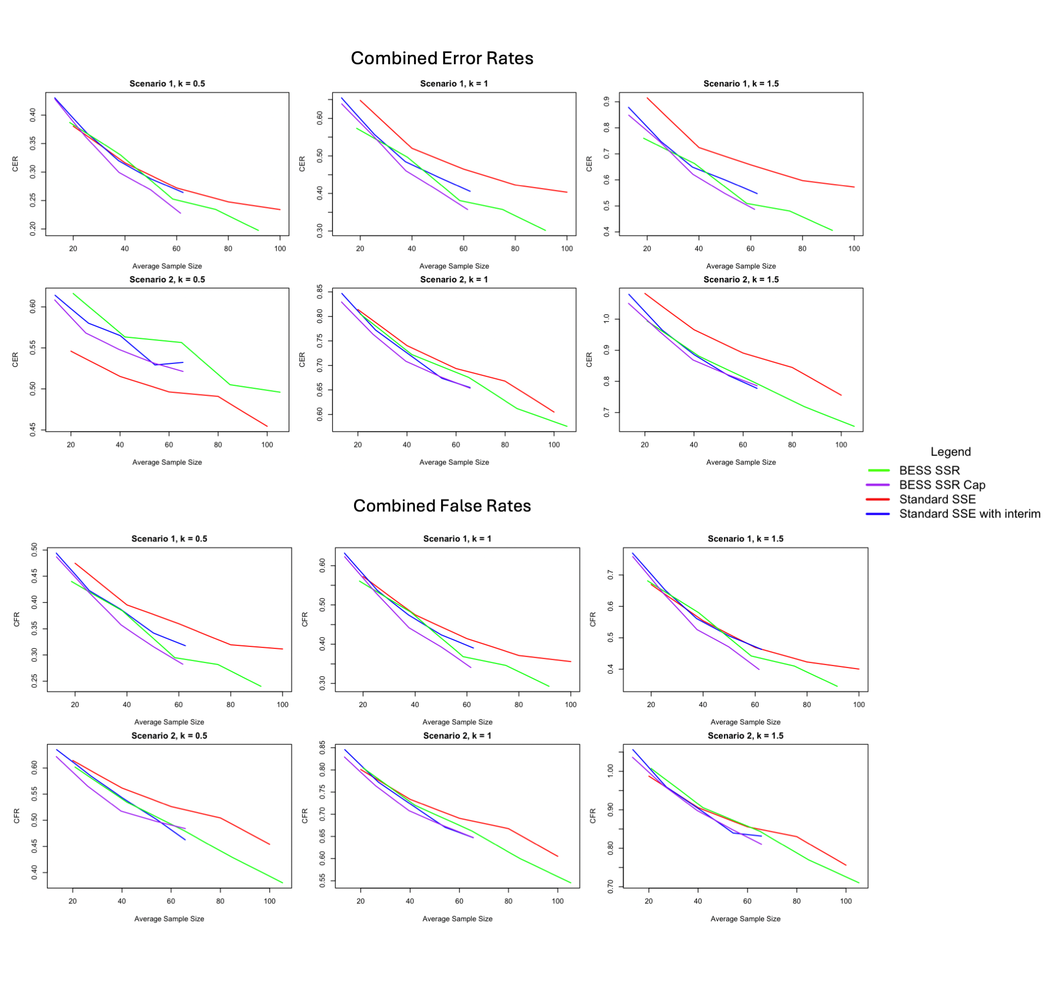
Figure 3: Combined Error Rates (CER) and Combined False Rates (CFR) across various sample sizes for the four designs under comparison. Different $k$ values are used to illustrate the importance of type I error rate over the type II error rate in CER or FPR over FNR in CFR.

Following Müller et al. (2004), we employ a loss function that integrates FPR and FNR into a single metric given by

$$\text{Combined False Rate (CFR)}=k\cdot\text{FPR}+\text{FNR}.$$

Again, $k\in\{0.5,1,1.5\}$. The results, shown in Figure 3, again suggest the BESS SSR Cap design (design 2) is the overall most desirable method. Therefore, to summarize, we recommend using the BESS with a sample size re-estimation capping the max sample size for the dose optimization trial.

7 Discussion

In this work we propose BESS as a new and simple Bayesian sample size estimator. BESS leads to a straightforward interpretation of estimated sample size: if the observed data exhibits certain level of evidence $e$ that supports the alternative hypothesis, with sample size $n$ one can conclude the alternative with confidence $c$, measured by posterior probability of the alternative. The statement is coherent with a subsequent Bayesian analysis of the trial using $n$ as the sample size. If the observed trial data exhibits evidence $e$, the posterior probability of alternative will be greater than $c$, corroborating with the sample size estimation. For dose optimization trials, the BESS SSR Cap design shows a superior performance under both Frequentist and Bayesian properties.

Simulation results show that for matched type I/II error rates and using vague priors, BESS produces similar sample size estimates as the standard Frequentist sample size estimation, even though the two are based on different philosophies and metrics. In addition, the preliminary comparison of various designs based on BESS suggests a slight advantage of the Bayesian approach.

Many future directions may be considered to further develop BESS and corresponding adaptive designs, such as group sequential designs with sample size re-estimations, and down-weight historical data in prior construction and decision rules for futility stopping, etc.

Appendix A

A.1 Posterior Probability of $H_{1}$ for One-arm Trial

In this subsection, we show for binary, continuous with known variance, and count-data outcomes in one-arm trial, the posterior probability of $H_{1}$ is a function of evidence $e$ as defined in equation (5) and sample size $n$, i.e., $\text{Pr}(H=H_{1}|\bm{y}_{n})=\text{Pr}(H=H_{1}|e,n)$.

Assume $\theta_{0}$ is a known constant, from Table (1) and equation (5), we have the posterior $f(\theta_{1}|\bm{y}_{n})$ in equation (3) for the three outcomes as follows:

• Binary:

  $$f(\theta_{1}|\bm{y}_{n})=\frac{\theta_{1}^{a+n\bar{y}}(1-\theta_{1})^{b+n(1-\bar{y})}}{B(a+n\bar{y},b+n(1-\bar{y}))}=\frac{\theta_{1}^{a+n[e+\theta_{0}]}(1-\theta_{1})^{b+n(1-[e+\theta_{0}])}}{B(a+n[e+\theta_{0}],b+n(1-[e+\theta_{0}]))}=f(\theta_{1}|e,n),$$

  where $B(\cdot,\cdot)$ is the beta function;

• Continuous with known $\sigma^{2}$:

  $$f(\theta_{1}|\bm{y}_{n})=\frac{1}{\sqrt{\frac{2\pi}{\frac{1}{b}+\frac{n}{\sigma^{2}}}}}\exp{\left\{-\frac{1}{2}\left[\frac{1}{b}+\frac{n}{\sigma^{2}}\right]\left(\theta_{1}-\frac{1}{\frac{1}{b}+\frac{n}{\sigma^{2}}}\left[\frac{a}{b}+\frac{n\bar{y}}{\sigma^{2}}\right]\right)^{2}\right\}}$$

  $$=\frac{1}{\sqrt{\frac{2\pi}{\frac{1}{b}+\frac{n}{\sigma^{2}}}}}\exp{\left\{-\frac{1}{2}\left[\frac{1}{b}+\frac{n}{\sigma^{2}}\right]\left(\theta_{1}-\frac{1}{\frac{1}{b}+\frac{n}{\sigma^{2}}}\left[\frac{a}{b}+\frac{n[e+\theta_{0}]}{\sigma^{2}}\right]\right)^{2}\right\}}=f(\theta_{1}|e,n),$$

• Count-data:

  $$f(\theta_{1}|\bm{y}_{n})=\frac{(b+n)^{a+n\bar{y}}}{\Gamma(a+n\bar{y})}\theta_{1}^{a+n\bar{y}}\exp{\{-(b+n)\theta_{1}\}}$$

  $$=\frac{(b+n)^{a+n[e+\theta_{0}]}}{\Gamma(a+n[e+\theta_{0}])}\theta_{1}^{a+n[e+\theta_{0}]}\exp{\{-(b+n)\theta_{1}\}}=f(\theta_{1}|e,n),$$

  where $\Gamma{(\cdot)}$ is the gamma function.

Hence, for all three outcomes in one-arm trial, we have $f(\theta_{1}|\bm{y}_{n})=f(\theta_{1}|e,n)$. As a result, when both $\theta_{0}$ and $\theta^{*}$ are given as fixed constants, we see that the integration term in equation (3) becomes a function of $e$ and $n$, i.e.,

$$g(e,n)=\int_{\theta_{1}-\theta_{0}>\theta^{*}}f(\theta_{1}|e,n)d\theta_{1}.$$

Consequently, equation (3) is a function of $e$ and $n$:

$$\text{Pr}(H=H_{1}|\bm{y}_{n})=\text{Pr}(H=H_{1}|e,n).$$

Note that $e$ here is the sufficient statistic for $\bm{y}_{n}$ for the three outcome types specified in this work.

A.2 Posterior Probability of $H_{1}$ for Two-arm Trial with Continuous outcome and known variance

Let $\bm{y}_{n}^{d}=\{y_{i}^{d};i=1,\ldots,n\}$ where $y_{i}^{d}=y_{i1}-y_{i0}$. Since $y_{ij}|\theta_{j}\sim N(\theta_{j},\sigma^{2}),\,j=0,1$ in model (2) for continuous outcome with known variance $\sigma^{2}$, which is common between $j=0$ and $j=1$, the likelihood of $y_{i}^{d}$ follows a normal distribution index by the parameters $\theta$ and $2\sigma^{2}$:

$$y_{i}^{d}|\theta\sim N(\theta,2\sigma^{2}),\,i=1,\ldots,n$$

Let $\pi=N(a,b)$ for $\theta$, we have:

$$\theta|H=H_{j}\sim N(a,b)I(\theta\in H_{j}),\,\,j=0,1,$$

and we have $\text{Pr}(H=H_{1})=q$ and $\text{Pr}(H=H_{0})=1-q$ as in model (2).

The posterior probability of $H_{1}$ is again given by equation (3), which we have

$$f(\bm{\theta}|\bm{y}_{n})=f(\theta|\bm{y}_{n}^{d})\propto f(\bm{y}_{n}^{d}|\theta)\pi(\theta).$$

Since the variance is known, and both $f(.)$ and $\pi(.)$ follows normal distribution, we have $f(\theta|\bm{y}_{n}^{d})$ follows a normal distribution and is similar to the continuous with known variance outcome in one-arm trial. Let $\bar{y}^{d}=\frac{1}{n}\sum_{i=1}^{n}y_{i}^{d}=\bar{y}_{1}-\bar{y}_{2}$, we have

$$f(\theta|\bm{y}_{n}^{d})=\frac{1}{\sqrt{\frac{2\pi}{\frac{1}{b}+\frac{n}{\sigma^{2}}}}}\exp{\left\{-\frac{1}{2}\left[\frac{1}{b}+\frac{n}{\sigma^{2}}\right]\left(\theta_{1}-\frac{1}{\frac{1}{b}+\frac{n}{\sigma^{2}}}\left[\frac{a}{b}+\frac{n\bar{y}^{d}}{\sigma^{2}}\right]\right)^{2}\right\}}$$

$$=\frac{1}{\sqrt{\frac{2\pi}{\frac{1}{b}+\frac{n}{\sigma^{2}}}}}\exp{\left\{-\frac{1}{2}\left[\frac{1}{b}+\frac{n}{\sigma^{2}}\right]\left(\theta_{1}-\frac{1}{\frac{1}{b}+\frac{n}{\sigma^{2}}}\left[\frac{a}{b}+\frac{ne}{\sigma^{2}}\right]\right)^{2}\right\}}=f(\theta_{1}|e,n),$$

where by equation (5), $\bar{y}^{d}=e$. With an argument similar to section A.1, we have

$$\text{Pr}(H=H_{1}|\bm{y}_{n})=\text{Pr}(H=H_{1}|e,n)$$

for the continuous with known variance outcome for two-arm trial.

A.3 Posterior Probability of $H_{1}$ for Two-arm Trial with Binary and Count-data Outcomes

From section A.1, we see that for $\theta_{j}$, $j=0,1$, we have $f(\theta_{j}|\bm{y}_{n})=f(\theta_{j}|\bar{y}_{j},n)$ for both the binary and count-data outcomes. Hence, we have

$$f(\bm{\theta}|\bm{y}_{n})=f(\theta_{0}|\bm{y}_{0n})f(\theta_{1}|\bm{y}_{1n})=f(\theta_{0}|\bar{y}_{0},n)f(\theta_{1}|\bar{y}_{1},n)=f(\bm{\theta}|\bar{y}_{1},\bar{y}_{0},n).$$

A.4 BESS Algorithm 2’

Below is BESS Algorithm 2’, where $\bar{y}_{1}$ and $\bar{y}_{0}$ are provided instead of evidence $e$.

BESS Algorithm 2’ Two-Arm Trials; Binary or Count Data

1:Input: The hierarchical models in Table 1.

2:Input: Clinically meaningful effect size $\theta^{*}$, response parameters for the treatment and control $\bar{y}_{1}$ and $\bar{y}_{0}$, confidence $c$, prior probability $q$.

3:Set $n_{\text{min}}$ and $n_{\text{max}}$ ($n_{\text{min}}<n_{\text{max}}$) the smallest and largest candidate sample sizes.

4:Set $n=n_{\text{min}}$.

5:while $n\leq n_{\text{max}}$ do

6:     Compute equation (3).

7:     if condition (7) is true then

8:         Stop and return the sample size $n$.

9:     else

10:         n = n+1

11:     end if

12:end while

13:if $n>n_{\text{max}}$ then

14:     Return sample size is larger than $n_{\text{max}}$.

15:end if

A.5 Simulation Parameters for Coherence in Section 4.2

Table A.1 shows the true parameters for data simulation in Section 4.2 to demonstrate coherence between BESS and Bayesian Inference.

Trial	Outcome	$\theta^{*}$	$\sigma^{2}$	$e$	$c$	$n$	$a$	$b$	True $\theta_{1}$	True $\theta_{0}$
Two-arm	Binary	0.05	-	0.1	0.8	150	0.5	0.5	0.3	0.2
	Continuous	0.1	0.5	0.2	0.8	71	0	10	0.8	0.6
	Count-data	0.3	-	0.4	0.8	100	1	2	0.7	0.3

Table A.1: Parameters for BESS, estimated sample size, and simulation truth for two-arm trial with all three outcome types. “-” means not applicable.

A.6 Additional Simulation Setup and Results in Section 5

Additional simulation details and results

Figure A.1 shows a flowchart for the simulation process in Section 5.1.

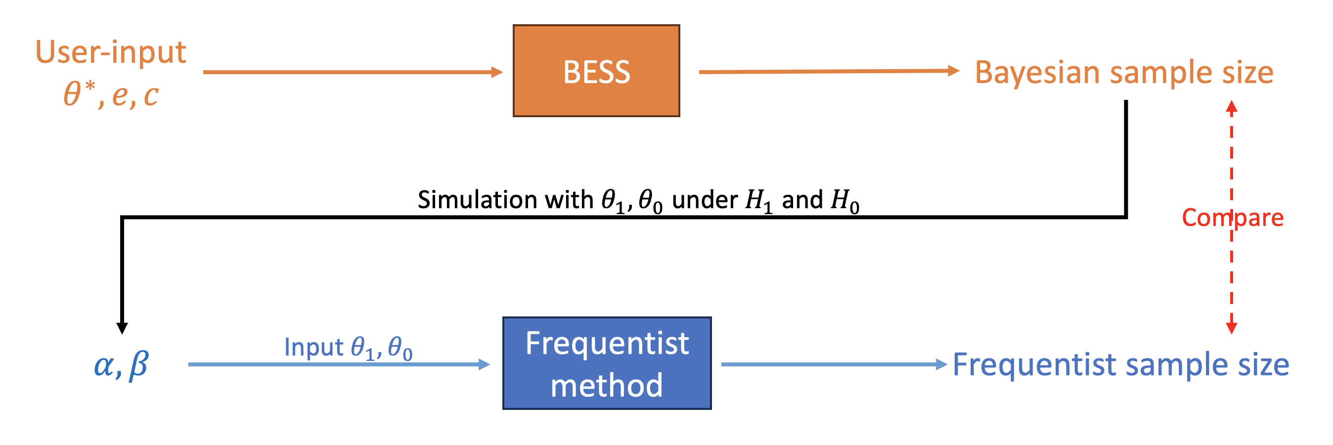
Figure A.1: Flowchart of simulation process to compare sample sizes estimated under BESS and that of the Frequenitst method.

Table A.2 show the results when $\theta_{0}$ and $\theta_{1}$ are mis-specified in the standard SSE.

Evidence	Confidence	Planned				Standard SSE	Simulation
$e$	$c$	$\theta_{1}$	$\theta_{0}$	$\alpha$	$1-\beta$	sample size $n$	$\alpha$	$1-\beta$	FPR	FNR
0.1	0.7	0.35	0.25	0.31	0.76	240	0.31	0.96	0.25	0.05
	0.8	0.35	0.25	0.20	0.84	560	0.20	1.00	0.17	0.00
	0.9	0.35	0.25	0.10	0.94	1136	0.10	1.00	0.09	0.00
0.2	0.7	0.45	0.25	0.44	0.57	3	0.37	0.49	0.43	0.45
	0.8	0.45	0.25	0.24	0.46	8	0.26	0.44	0.37	0.42
	0.9	0.45	0.25	0.11	0.38	17	0.14	0.30	0.31	0.44

Table A.2: Standard SSE sample size and simulated Type I error rate, power, false positive rate, and false negative rate when $\theta_{1}-\theta_{0}$ is mis-specified by the Frequentist method to match $e$ in BESS for two-arm trial with binary outcome.

Additional simulation details in sensitivity of prior

In the previous simulation, we assume a flat prior $\text{Beta}(0,0)$ for BESS. In particular, this prior is used to find the sample size as well as to compute $\text{Pr}(H=H_{1}|\bm{y}_{n})$ for each simulated trial. In Morita et al. [2008], the authors show that the prior effective sample size of $\text{Beta}(a,b)$ for a binomial likelihood is quantified as $(a+b).$ Therefore, $\text{Beta}(0,0)$ is considered noninformative in that it includes no prior information for the posterior inference.

However, BESS can accommodate prior information, if available, as part of sample size estimation. Assuming there exist $n_{0}$ patients per arm as prior data, we demonstrate the sensitivity of incorporating these prior information through simulation. First consider the simulation process for a single trial with the following two steps: 1) generating the prior data, 2) assume evidence $e=0.15$ and $c=0.8$, estimate the sample size via BESS using the informative priors constructed from the prior data. For step 1, assuming there are $n_{0}=10$ external patients data per arm that is available to be incorporated, we generate these prior data similar to the simulation process in Section 5.1 with $\theta_{1}=0.4$ and $\theta_{0}=0.25$. Denote the generated data $\bm{y}_{j}^{0}=\{y_{ij}^{0};i=1,\ldots,n_{0}\},\,j=1,0$ as the binary outcomes of these 10 patients’ external data for the treatment and the control arms, respectively. We consider an informative prior for BESS as

$$(\theta_{1},\theta_{0})|H=H_{j}\sim\prod_{j=1}^{2}\text{Beta}\left(\sum_{i=1}^{n_{0}}y_{ij}^{0},n_{0}-\sum_{i=1}^{n_{0}}y_{ij}^{0}\right)I\{(\theta_{1},\theta_{0})\in H_{j}\}.$$

We find sample size via BESS’s algorithm 2 with the informative prior, $e$, and $c$. Following this process, we simulate 1,000 trials and compute the average sample size to compare to BESS with vague prior.

A.7 Metrics Used in Section 6.2

The metrics include: 1) Type I error rate, 2) Type II error rate, 3) False positive rate, and 4) False negative rate. These rates are defined below:

Type I error rate: proportion of simulated trials in which the null is true but falsely rejected:

$$\text{Type I error rate}=\frac{\#\text{ reject simulation trials in null}}{\#\text{ simulation trials in null}}.$$

Type II error rate: proportion of simulated trials in which the alternative is true but falsely rejected:

$$\text{Type II error rate}=\frac{\#\text{ accept simulation trials in alternative}}{\#\text{ simulation trials in alternative}}.$$

False positive rate (FPR): proportion of simulated trials in which the null is rejected but true:

$$\text{FPR}=\frac{\#\text{ reject simulation trials in null}}{\#\text{ reject simulation trials}}.$$

False negative rate (FNR): proportion of simulated trials in which the null is accepted but not true:

$$\text{FNR}=\frac{\#\text{ accept simulation trials in alternative}}{\#\text{ accept simulation trials}}.$$

A.8 BESS Software and Verification

Package description

The R functions are available at https://ccte.uchicago.edu/bess. For one-arm trials, there are two functions:

• BESS_one_arm($\theta^{*}$, $c$, $e$, outcome, $a$, $b$, $q$, $\sigma$, $n_{\text{min}}$, $n_{\text{max}}$)

  • Parameters:

    $\theta^{*}$	Clinically minimum effect margin
    $c$	Confidence threshold
    $e$	Assumed evidence
    outcome	Outcome type: 1 = binary, 2 = continuous, 3 = count-data
    $a$, $b$	Hyperparameters for $\pi_{1}$
    $q$	Prior probability of $H_{1}$, default to 0.5
    $\sigma$	Known variance when outcome is continuous. For other outcomes, it is not used. The default value is 1.
    $n_{\text{min}}$, $n_{\text{max}}$	Minimum and maximum sample sizes for the searching algorithm.

  • Description: BESS algorithm 1 for the three outcomes in one-arm trial.

  • Output: Sample size in the treatment arm for the three outcomes in one-arm trial.

• post_prob_H1_1a($n$, $\theta^{*}$, $e$, outcome, $a$, $b$, $\sigma$, $q$)

  • Parameters:

    $n$	Sample size per arm
    $\theta^{*}$	Clinically minimum effect margin
    $e$	Assumed or observed evidence from data
    outcome	Outcome type: 1 = binary, 2 = continuous, 3 = count-data
    $a$, $b$	Hyperparameters for $\pi_{1}$
    $\sigma$	Known variance when outcome is continuous. For other outcomes, it is not used. The default value is 1.
    $q$	Prior probability of $H_{1}$, default to 0.5

  • Description: Compute the posterior probability of alternative (equation (3)) for the three outcome types of one arm trial.

  • Output: Posterior probability of $H_{1}$ (confidence) given sample size $n$, evidence $e$, and clinically minimum effect size $\theta^{*}$.

For two-arm trials, there are six functions:

• BESS_bin($\theta^{*}$, $c$, $e$, $n_{\text{min}}$, $n_{\text{max}}$, $a_{1}$, $b_{1}$, $a_{2}$, $b_{2}$, $q$, sim)

  • Parameters:

    $\theta^{*}$	Clinically minimum effect margin
    $c$	Confidence threshold
    $e$	Assumed evidence
    $n_{\text{min}}$, $n_{\text{max}}$	Minimum and maximum sample sizes for the searching algorithm
    $a_{1}$, $b_{1}$, $a_{2}$, $b_{2}$	Hyperparameters for $\pi_{1}$ and $\pi_{0}$
    $q$	Prior probability of $H_{1}$, default to 0.5
    sim	Simulation numbers to compute posterior probability of $H_{1}$ through a simulation approach, default to 10,000

  • Description: BESS algorithm 2 for binary outcomes in two-arm trial.

  • Output: Sample size per arm for binary outcomes in two-arm trial.

• BESS_cont($\theta^{*}$, $c$, $e$, $a$, $b$, $n_{\text{min}}$, $n_{\text{max}}$, $q$, $\sigma$)

  • Parameters:

    $\theta^{*}$	Clinically minimum effect margin
    $c$	Confidence threshold
    $e$	Assumed evidence
    $a$, $b$	Hyperparameters for prior in two-arm continuous outcome
    $n_{\text{min}}$, $n_{\text{max}}$	Minimum and maximum sample sizes for the searching algorithm
    $q$	Prior probability of $H_{1}$, default to 0.5
    $\sigma$	Known variance for each arm when outcome is continuous, assuming same variance. For other outcomes, it is not used. The default value is 1.

  • Description: BESS algorithm 1 for continuous outcomes with known variance in two-arm trial.

  • Output: Sample size per arm for continuous outcomes with known variance in two-arm trial.

• BESS_count($\theta^{*}$, $c$, $e$, $a_{1}$, $b_{1}$, $a_{2}$, $b_{2}$, $n_{\text{min}}$, $n_{\text{max}}$, $q$, sim)

  • Parameters:

    $\theta^{*}$	Clinically minimum effect margin
    $c$	Confidence threshold
    $e$	Assumed evidence
    $a_{1}$, $b_{1}$, $a_{2}$, $b_{2}$	Hyperparameters for $\pi_{1}$ and $\pi_{0}$
    $n_{\text{min}}$, $n_{\text{max}}$	Minimum and maximum sample sizes for the searching algorithm
    $q$	Prior probability of $H_{1}$, default to 0.5
    sim	Simulation numbers to compute posterior probability of $H_{1}$ through a simulation approach, default to 10,000

  • Description: BESS algorithm 2 for count outcomes in two-arm trial.

  • Output: Sample size per arm for count outcomes in two-arm trial.

• post_prob_H1_sim($y_{1}$, $y_{0}$, $n$, $\theta^{*}$, $a_{1}$, $b_{1}$, $a_{2}$, $b_{2}$, $q$, sim)

  • Parameters:

    $y_{1}$, $y_{0}$	The number of responders out of $n$ patients in the treatment and control arms
    $n$	Sample size per arm
    $\theta^{*}$	Clinically minimum effect margin
    $a_{1}$, $b_{1}$, $a_{2}$, $b_{2}$	Hyperparameters for $\pi_{1}$ and $\pi_{0}$
    $q$	Prior probability of $H_{1}$, default to 0.5
    sim	Simulation numbers to compute posterior probability of $H_{1}$ through a simulation approach, default to 10,000

  • Description: Compute the posterior probability of alternative (equation (3)) for binary outcome in two-arm trial.

  • Output: Posterior probability of $H_{1}$ (confidence) given sample size $n$, responders in treatment and control arms, and clinically minimum effect size $\theta^{*}$.

• post_prob_H1_cont($n$, $\theta^{*}$, $e$, $a$, $b$, $\sigma$, $q$)

  • Parameters:

    $n$	Sample size per arm
    $\theta^{*}$	Clinically minimum effect margin
    $e$	Assumed or observed evidence from data
    $a$, $b$	Hyperparameters for prior in two-arm continuous outcome
    $\sigma$	Known variance for each arm when outcome is continuous, assuming same variance. For other outcomes, it is not used. The default value is 1.
    $q$	Prior probability of $H_{1}$, default to 0.5

  • Description: Compute the posterior probability of alternative (equation (3)) for continuous outcome in two-arm trial.

  • Output: Posterior probability of $H_{1}$ (confidence) given sample size $n$, difference in mean responses between treatment and control arms, and clinically minimum effect size $\theta^{*}$.

• post_prob_H1_cnt_sim($y_{1}$, $y_{0}$, $n$, $\theta^{*}$, $a_{1}$, $b_{1}$, $a_{2}$, $b_{2}$, $q$, sim)

  • Parameters:

    $y_{1}$, $y_{0}$	The observed events in treatment and control arms
    $n$	Sample size per arm
    $\theta^{*}$	Clinically minimum effect margin
    $a_{1}$, $b_{1}$, $a_{2}$, $b_{2}$	Hyperparameters for $\pi_{1}$ and $\pi_{0}$
    $q$	Prior probability of $H_{1}$, default to 0.5
    sim	Simulation numbers to compute posterior probability of $H_{1}$ through a simulation approach, default to 10,000

  • Description: Compute the posterior probability of alternative (equation (3)) for count outcome in two-arm trial.

  • Output: Posterior probability of $H_{1}$ (confidence) given sample size $n$, event rates in treatment and control arms, and clinically minimum effect size $\theta^{*}$.

Moreover, there are also two functions to obtain the simulation results for the four designs in Section 6.2:

• BESS_SSR_bin_design($\theta_{H}$, $\theta_{L}$, $\theta^{*}$, $c$, $c^{*}$, $n_{0}$, $a_{1}$, $b_{1}$, $a_{2}$, $b_{2}$, $q$, $n_{\text{min}}$, $n_{\text{max}}$, cap, $n_{\text{cap}}$)

  • Parameters:

    $\theta_{H}$, $\theta_{L}$	Simulation truth for the response rates in the higher and lower doses
    $\theta^{*}$	Noninferiority margin
    $c$, $c_{s}$	Thresholds for success and futility
    $n_{0}$	Number of patients at interim
    $a_{1}$, $b_{1}$, $a_{2}$, $b_{2}$	Hyperparameters for $\pi_{1}$ and $\pi_{0}$
    $q$	Prior probability of $H_{1}$, default to 0.5
    $n_{\text{min}}$, $n_{\text{max}}$	Minimum and maximum sample sizes for the searching algorithm
    cap	Indicator whether to limit the maximum sample size. cap = F is BESS SSR design, cap = T is BESS SSR with Cap design Default to cap = F.
    $n_{\text{cap}}$	The maximum allowed sample size per arm

  • Description: The BESS SSR and BESS SSR with Cap design for a single simulation.

  • Output: Design’s decision and sample size.

• StandardSSE_bin_design($n_{f}$, $\theta_{H}$, $\theta_{L}$, $\theta^{*}$, $\alpha$, interim, $n_{0}$, $a_{1}$, $b_{1}$, $a_{2}$, $b_{2}$, $q$, $c$, $c^{*}$)

  • Parameters:

    $n_{f}$	Total sample size per arm in Standard SSE design
    $\theta_{H}$, $\theta_{L}$	Simulation truth for the response rates in the higher and lower doses
    $\theta^{*}$	Noninferiority margin
    $\alpha$	Significant level for z-test
    interim	Indicator if there is an interim, default to False
    $n_{0}$	Number of patients at interim
    $a_{1}$, $b_{1}$, $a_{2}$, $b_{2}$	Hyperparameters for $\pi_{1}$ and $\pi_{0}$
    $q$	Prior probability of $H_{1}$, default to 0.5
    $c$, $c_{s}$	Thresholds for success and futility

  • Description: The Standard SSE and Standard SSE with Interim designs for a single simulation.

  • Output: Design’s decision and sample size.

Package validation

The results in the main manuscript verified the coherence property for two-arm trials. Moreover, an example which compares BESS sample size to the Standard SSE based on matched Type I/II error rates is demonstrated for binary outcome in a two-arm trial. The four designs functions are also showed in the main manuscript in Section 6.2. Here, we verify the coherence property and demonstrate similar sample sizes between BESS and standard SSE for binary outcome in one-arm trial as an example for one-arm trials.

To show the coherence property of one-arm trials, we first use BESS to estimate the sample sizes for the three outcomes in one-arm trial, with $e=0.4$, $\theta_{0}=0$, $\theta^{*}=0.3$, and $c=0.8$. We obtained 15 patients for binary outcome, 71 for continuous outcome, and 25 for count outcome. Next, following Section 4.2, we obtain a similar plot as Figure 2 in the manuscript, shown in Figure A.2, for the three outcomes in one-arm trial. The result suggests the coherence property of BESS for one-arm trial, which verifies the one-arm trial functions.

The following code segments uses BESS to estimate the sample sizes and produces Figure A.2:

⬇

set.seed(1234)

theta1 <- 0.4

theta0 <- 0

theta_s <- 0.3

e <- 0.4

c <- 0.8

> BESS_one_arm(theta_s, c, e, 1, 0.5, 0.5)\$n

[1] 15

> BESS_one_arm(theta_s, c, e, 2, 0, 10)\$n

[1] 71

> BESS_one_arm(theta_s, c, e, 3, 1, 2)\$n

[1] 25

show_cohorence <- function(theta1, theta0, theta_s, e, c, n, a, b,

outcome, subv, main, sig = 1, q = 0.5,

n_sim = 10000){

sim_arr <- matrix(rep(NA, 2*n_sim),ncol=2)

for(i in 1:n_sim){

if(outcome == 1){

yi_trt <- rbinom(n, 1, prob = theta1)

yd <- mean(yi_trt) - theta0

}else if(outcome == 2){

yi_trt <- rnorm(n, mean = theta1, sd = sig)

yd <- mean(yi_trt) - theta0

}else{

yi_trt <- rpois(n, lambda = theta1)

yd <- mean(yi_trt) - theta0

}

post_H1 <- post_prob_H1_1a(n, theta_s, yd, outcome,

a, b, sig = sig, q = q)

sim_arr[i,] <- c(yd,post_H1)

}

smoothScatter(sim_arr[,1], sim_arr[,2],

xlab = paste0(”Evidence \n ”,subv),

ylab = ”Confidence”, bandwidth = 0.007,

nrpoints = 0, main = main)

abline(v = e, col = ”black”, lty = 2)

abline(h = c, col = ”red”, lty = 3)

}

show_cohorence(theta1, theta0, theta_s, e, c, 15, 0.5, 0.5, 1,

”(a)”, ”Binary outcome”)

show_cohorence(theta1, theta0, theta_s, e, c, 71, 0, 10, 2,

”(b)”, ”Continuous outcome”)

show_cohorence(theta1, theta0, theta_s, e, c, 25, 1, 2, 3,

”(c)”, ”Count-data outcome”)

Figure A.2: Plots of observed confidence $c^{\star}$ vs. observed evidence $e^{\star}$ for binary, continuous, and count-data outcomes with one-arm trial. The black vertical dashed line shows the location of $e^{\star}=e$, and the red horizontal dotted line shows the location of $c^{\star}=c$.

Lastly, we verify the BESS methods for each trial and outcome types and show that similar sample sizes may be obtained with BESS and with standard SSE when the Type I and Type II error rates are matched. Following the simulation process in Section 5, the following code segments computes the Type I error rate and power (1 - Type II error rate) through simulation for one arm trials:

⬇

c, n, a, b, outcome = 1, sig = 1, q = 0.5,

n_sim = 10000){

result_arr <- matrix(rep(NA, 2*n_sim),ncol=2)

for(i in 1:n_sim){

if(outcome == 1){

yi_trtH1 <- rbinom(n, 1, prob = theta1H1)

yi_trtH0 <- rbinom(n, 1, prob = theta1H0)

}else if(outcome == 2){

yi_trtH1 <- rnorm(n, mean = theta1H1, sd = sig)

yi_trtH0 <- rnorm(n, mean = theta1H0, sd = sig)

}else{

yi_trtH1 <- rpois(n, lambda = theta1H1)

yi_trtH0 <- rpois(n, lambda = theta1H0)

}

ydH1 <- mean(yi_trtH1) - theta0

ydH0 <- mean(yi_trtH0) - theta0

post_H1_H1 <- post_prob_H1_1a(n, theta_s, ydH1, outcome,

a, b, sig = sig, q = q)

dec_H1 <- 0

if(post_H1_H1 >= c){

dec_H1 <- 1

}

post_H1_H0 <- post_prob_H1_1a(n, theta_s, ydH0, outcome,

a, b, sig = sig, q = q)

dec_H0 <- 0

if(post_H1_H0 >= c){

dec_H0 <- 1

}

result_arr[i,] <- c(dec_H0, dec_H1)

}

TIER <- sum(result_arr[,1] == 1)/n_sim

power <- sum(result_arr[,2] == 1)/n_sim

return(c(TIER, power))

}

> freq_prop_one_arm(0.4, 0.3, 0, 0.3, 0.8, 60,

0.5, 0.5, outcome = 1, n_sim = 1000)

[1] 0.2363 0.8278

For two-arm trials, the control arm’s data is also drawn from their respective distributions. The Frequentist sample size is then estimated using standard sample size packages such as “TrialSize” or online software. Table A.3 shows the estimated sample sizes via BESS and the oracle sample size with the standard SSE method. Again, the observation is similar to Table 2 in the manuscript, and further verifies these functions.

Table A.3: Simulation results compare BESS with Standard SSE when the Type I error rate and power are matched between both methods in one- and two-arm trial with all three outcomes. The results show the estimated sample sizes of the two methods are similar for various levels of evidence $e$ and confidence $c$ in each trial and outcome type.

Trail	Outcome	Evidence	Confidence	type I	power	BESS	Standard SSE
type	type	$e$	$c$	error rate $\alpha$	$1-\beta$	$n$	$n$
One-arm	Binary	0.35	0.8	0.24	0.83	60	63
	Continuous	0.4	0.8	0.20	0.50	71	71
	Count	0.375	0.8	0.20	0.64	40	41
Two-arm	Binary	0.20	0.9	0.11	0.38	35	36
	Continuous	0.15	0.8	0.20	0.40	32	33
	Count	0.3	0.7	0.27	0.88	51	51

References

- Adcock [1997] CJ Adcock. Sample size determination: a review. Journal of the Royal Statistical Society: Series D (The Statistician), 46(2):261–283, 1997.
- Berry et al. [2010] Scott M Berry, Bradley P Carlin, J Jack Lee, and Peter Muller. Bayesian adaptive methods for clinical trials. CRC press, 2010.
- Blumenthal et al. [2021] Gabriel Blumenthal, Lakhmir Jain, Amy L Loeser, Yogesh K Pithaval, Arshad Rahman, Mark J Ratain, Manish Shah, Laurie Strawn, and Marc R Theoret. Optimizing dosing in oncology drug development. Friends Cancer Res, pages 1–14, 2021.
- Ciarleglio and Arendt [2017] Maria M Ciarleglio and Christopher D Arendt. Sample size determination for a binary response in a superiority clinical trial using a hybrid classical and bayesian procedure. Trials, 18:1–21, 2017.
- Desu [2012] MM Desu. Sample size methodology. Elsevier, 2012.
- Food et al. [2023] US Food, Drug Administration, et al. Project optimus: Reforming the dose optimization and dose selection paradigm in oncology. Food and Drug Administration, 2023.
- Hobbs et al. [2011] Brian P Hobbs, Bradley P Carlin, Sumithra J Mandrekar, and Daniel J Sargent. Hierarchical commensurate and power prior models for adaptive incorporation of historical information in clinical trials. Biometrics, 67(3):1047–1056, 2011.
- Ibrahim and Chen [2000] J.G Ibrahim and M.H Chen. Power prior distributions for regression models. Statistical Science, pages 46–60, 2000.
- Inoue et al. [2005] Lurdes YT Inoue, Donald A Berry, and Giovanni Parmigiani. Relationship between bayesian and frequentist sample size determination. The American Statistician, 59(1):79–87, 2005.
- Kim and Choi [2021] Jae H Kim and In Choi. Choosing the level of significance: A decision-theoretic approach. Abacus, 57(1):27–71, 2021.
- Kunzmann et al. [2021] Kevin Kunzmann, Michael J Grayling, Kim May Lee, David S Robertson, Kaspar Rufibach, and James MS Wason. A review of bayesian perspectives on sample size derivation for confirmatory trials. The American Statistician, 75(4):424–432, 2021.
- Lee and Zelen [2000] Sandra J Lee and Marvin Zelen. Clinical trials and sample size considerations: another perspective. Statistical science, 15(2):95–110, 2000.
- Lin et al. [2022] Xiaolei Lin, Jiaying Lyu, Shijie Yuan, Dehua Bi, Sue-Jane Wang, and Yuan Ji. Bayesian sample size planning tool for phase i dose-finding trials. JCO Precision Oncology, 6:e2200046, 2022.
- Morita et al. [2008] Satoshi Morita, Peter F Thall, and Peter Müller. Determining the effective sample size of a parametric prior. Biometrics, 64(2):595–602, 2008.
- Müller et al. [2004] Peter Müller, Giovanni Parmigiani, Christian Robert, and Judith Rousseau. Optimal sample size for multiple testing: the case of gene expression microarrays. Journal of the American Statistical Association, 99(468):990–1001, 2004.
- Shah et al. [2021] Mirat Shah, Atiqur Rahman, Marc R Theoret, and Richard Pazdur. The drug-dosing conundrum in oncology-when less is more. The New England journal of medicine, 385(16):1445–1447, 2021.
- Wang and Ji [2020] Xiaofeng Wang and Xinge Ji. Sample size estimation in clinical research: from randomized controlled trials to observational studies. Chest, 158(1):S12–S20, 2020.
- Wittes [2002] Janet Wittes. Sample size calculations for randomized controlled trials. Epidemiologic reviews, 24(1):39–53, 2002.