Controlling measurement induced phase transitions with tunable detector coupling

Abstract

We study the evolution of a quantum many-body system driven by two competing measurements, which induces a topological entanglement transition between two distinct area law phases. We employ a positive operator-valued measurement with variable coupling between the system and detector within free Fermion dynamics. This approach allows us to continuously track the universal properties of the transition between projective and continuous monitoring. Our findings suggest that the percolation universality of the transition in the projective limit is unstable when the system-detector coupling is reduced.

Introduction- In recent years, there has been a significant surge of interest in investigating the spread of quantum information within open many-body quantum systems. This interest spans areas like quantum computation and teleportation,condensed matter theory, and statistical physics, The environment acts as a measurement apparatus, continuously probing the system [1, 2]. These repeated measurements restrict the entanglement growth and corrupt the quantum information, leading to a measurement-induced phase transition marked by a sudden shift in the scaling of entanglement entropy [3, 4, 5, 6, 7, 8, 9, 4], reported in cutting edge experiments[10, 11, 12].

Entanglement transitions can also arise in a system subjected to competing measurements. Here, the competition between the two measurements drives a topological entanglement transition between distinct disentangled phases. This procedure can be used to tailor quantum states with distinct topological order [13, 14, 15, 16, 17, 18, 19] which can be potentially useful for quantum error correction observed in recent cutting-edge experiments [20, 21]. The critical properties of topological entanglement transition under projective measurement differ considerably from those driven by continuous weak monitoring  [13, 22, 19, 23]. However, how the criticality depends on the detailed coupling to the environment beyond these two limits is yet to be explored.

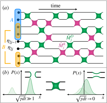
Figure 1: (a) Space-time schematic of measurements $\hat{M}^{D}$, $\hat{M}^{K}$ on the Majorana (free fermionic) chain with probability $p^{D}$, $p^{K}$ and strength $\gamma^{D}$, $\gamma^{K}$, respectively. The two partitions of chains A and B contribute to calculating topological entanglement entropy ($S_{T}$). (b) The initial Gaussian state of the detector associated with any measurement operator is modified, which depends on the strength of the measurement ($\sqrt{\gamma dt}$) shown by the probability distribution P(x) (Eq.(2)).

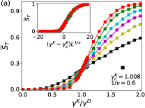
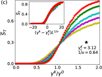
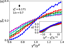
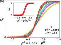
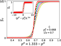
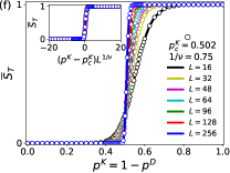
Figure 2: The averaged topological entanglement entropy ($\bar{S}_{T}$) in units of $\log 2$ as a function of (a,c,e) relative measurement strength ($\gamma^{K}/\gamma^{D}$) and (b,d,f) probabilities ($p^{K},\;p^{D}$) of the two competing measurements $\hat{M}^{K}$ and $\hat{M}^{D}$ for different system sizes. All the inset shows the scaling across the critical points ($\gamma^{K}_{c}$ or $p^{K}_{c}$) with the corresponding scaling exponents ($\nu$) shown in Fig. 3 of the respective figures. The details of different parameters for all cases follow are: ($\blacksquare$) $\gamma^{D}=1$, $p^{D}=p^{K}=1$, ($\bigstar$) $\gamma^{D}=\gamma^{K}=3$, $p^{K}+p^{D}=1.667$, ($\largestar$) $\gamma^{D}=3$, $p^{D}=p^{K}=0.833$, ($\Diamondblack$) $\gamma^{D}=\gamma^{K}=6$, $p^{K}+p^{D}=1.333$, ($\Diamond$) $\gamma^{D}=6$, $p^{D}=p^{K}=0.667$, ($\circ$) $\gamma^{D}=\gamma^{K}=9$, $p^{K}+p^{D}=1$. The time steps for different cases are (a) $dt=0.05$, (b-f) $dt=1$.

To address this question, we explore the evolution of topological order within a measurement-only dynamics framework. We consider two competing measurements: one that creates entanglement between neighboring sites and another that disentangles a local site from the rest of the system, thereby giving rise to distinct area-law phases. We illustrate that the previously studied projective and weak continuous monitoring can manifest as limiting behaviors within a unified framework of general positive operator-valued measurements (POVM) with variable system-detector coupling. Importantly, this general POVM can be implemented within a framework of a free fermion chain.

Our findings reveal that the percolation universality that describes the transition in the projective limit, is unstable to reducing the coupling between system and detector. In particular, adjusting the coupling strength continuously modifies the finite size scaling exponent of the transition.

Model and methodology – The study of the measurement-induced entanglement transitions predominantly falls into two classes: quantum circuits with unitary gates disrupted by projective measurements [6, 5, 3, 4], and systems evolving under continuous measurement and Hamiltonian dynamics [24, 25, 26]. However, it is possible to adopt a more general perspective to explore a wider range of environments, whereby measurements are described by POVMs  [27, 1, 28]. In particular, one can consider POVMs with a controlled back-action, in which the system is coupled to a detector through a unitary evolution, causing the system and the detector to become entangled. A projective measurement of the detector induces a back-action on the system. If the coupling is strong, this is akin to a projective measurement of the state of the system. If, however, the system and detector are weakly coupled, the detector obtains very little information on the state of the system, causing a weak backaction that depends non-linearly on the state itself.

Implementing these POVM operations in the system requires integration/connection with external detectors, which provide a continuous spectrum of outcomes utilized as stochastic back-action onto the system [8, 25]. Hence, the dynamics governing the interaction of the system with any measurement $\hat{M}$ coupled to this external detector is expressed by $e^{i\lambda\hat{M}\otimes\hat{p}}|\psi\rangle\otimes|\phi\rangle$, where $|\psi\rangle$, $|\phi\rangle$ are the initial state of the system and the detector, respectively. Here, $\lambda$ is the effective measurement strength ($\lambda=\sqrt{\gamma dt}$, where $\gamma$ is the measurement strength of $\hat{M}$), and $\hat{p}$ is the momentum conjugate to the position, $\hat{x}$ of the detector/pointer. Therefore, the detector dynamics can be tracked down with $\hat{\dot{x}}=\lambda\hat{M}$, where $x$ represents the position of the detector.

Here, we consider the detector as a one-dimensional pointer prepared in a Gaussian state centered around zero with variance given by $\Delta^{2}$: $|\phi\rangle=\int dx\sqrt{G_{\Delta}(x)}|x\rangle$, where $G_{\Delta}(x)=\exp(-x^{2}/2\Delta^{2})/(\sqrt{2\pi}\Delta)$. This pointer is linearly coupled to a local measurement operator $\hat{M}=\sum_{\ell}m_{\ell}\hat{\Pi}_{\ell}$, where $m_{\ell}$ represents the $\ell^{th}$ eigenvalue of the operator $\hat{M}$ and $\hat{\Pi}_{\ell}$ stands for the projector onto the corresponding eigenvector. When the detector is projectively measured, the pre-measurement state of the system $|\psi\rangle$, is updated to $|\psi^{\prime}\rangle$ via [1, 28]:

$$|\psi^{\prime}\rangle=\frac{\hat{K}(x,\lambda,\Delta)}{\sqrt{P(x)}}|\psi\rangle.$$ (1)

where $\hat{K}(x,\lambda,\Delta)=\sum_{\ell}\sqrt{G_{\Delta}(x-\lambda m_{\ell})}\hat{\Pi}_{\ell}$ is the Kraus operator associated with the outcome $x$, of the position measurement on the detector. The normalization is given by the probability to obtain the outcome $x$ from the measurement:

$$P(x)=\langle\psi|\hat{K}^{\dagger}(x,\lambda,\Delta)\hat{K}(x,\lambda,\Delta)|\psi\rangle.$$ (2)

The choice of coupling strength $\lambda$ allows us to explore the effect of the degree of entanglement between system and detector on the dynamics. In particular, in the commonly studied weak measurement scenario ($\lambda=\sqrt{\gamma dt}\ll\Delta$), the separation between the Gaussian distributions in Eq. 2 is small as shown in right panel of Fig. 1(b) and can be approximated by a single Gaussian distribution $G_{\Delta}(x-\lambda\langle\hat{M}\rangle)$ with a shifted mean value which depends on the state $\lambda\langle\hat{M}\rangle$. In this scenario, the back action resulting from the measurement is akin to a Wiener process [1] and produces dynamics equivalent to the Stochastic Schrödinger’s equation [26, 28, 29], as given by:

$$|\psi^{\prime}\rangle\approx\frac{1}{N}e^{(\delta W_{t}+\lambda^{2}\langle\hat{M}\rangle)\hat{M}}|\psi\rangle,$$ (3)

where $\delta W_{t}$ represents Wiener stochastic increments that are independently Gaussian-distributed with $\langle\delta W_{t}\rangle=0$ and $\langle\delta W_{t}\delta W_{t^{\prime}}\rangle=\lambda^{2}\delta_{t,t^{\prime}}$.

Conversely, in the case of strong measurement ($\lambda\gg\Delta$), the distribution of detector outcomes consists of a sum of separated Gaussians with exponentially small overlap, as illustrated in the left panel of Fig. 1(b). Consequently, the outcome of the detector feedback on the system is dominated by a one eigenvector projection over all others of the measurement $\hat{M}$. The resulting dynamics are exponentially close to that of a projective measurement.

The above discussion is general and can be applied to any many-body system subjected to the monitoring of local operators. However, the numerical implementation of a weighted sum of projectors is, generically, challenging. Nonetheless, numerical tractability can be achieved in a free Fermion system evolving under weak continuous [26, 19, 30, 31] or in Clifford gates subjected to projective monitoring [5, 13, 14, 2]. We note, however, measurements that satisfy $\hat{M}^{2}=\hat{M}$ or $\hat{M}^{2}=\hat{\mathbb{I}}$ preserve the gaussianity of the state. Hence, in free Fermions it is possible to express the Kraus operator for general system and detector coupling strength as:

$$|\psi_{t+dt}\rangle = \frac{1}{N}e^{\frac{\lambda P^{M}x\hat{M}}{2\Delta^{2}}}|\psi_{t}\rangle,$$ (4)

where we have added a probability $P^{M}\in\{0,1\}$ to perform the given measurement.

With a comprehensive understanding of POVMs, we now shift our focus to our system of interest. We study measurement-only dynamics driven by two non-commuting positive operator value measurements on a one-dimensional spinless free fermionic chain (Majorana string) of length $L$ as shown in Fig. 1(a). The two types of measurements correspond to local density and Kitaev-type bond density and can be expressed as staggered pairwise parity checks on the Majorana chain:

$$\hat{M}^{D}_{j} =c^{\dagger}_{j}c_{j}-c_{j}c^{\dagger}_{j}=i\eta_{2j}\eta_{2j-1}$$ (5)

$$\hat{M}^{K}_{j} =\left(c_{j}+c_{j}^{\dagger}\right)\left(c_{j+1}-c_{j+1}^{\dagger}\right)=i\eta_{2j}\eta_{2j+1}$$ (6)

where $c_{j}=\frac{1}{2}\left(\eta_{2j}+i\eta_{2j-1}\right)$ is fermionic annihilation operator on the $j^{th}$ site. The measurement strength is controlled by parameters $\gamma^{D}$ and $\gamma^{K}$, respectively. The eigenvalues of each measurement are $1,-1$ with the corresponding projectors given by $\hat{\Pi}^{D}_{j,\pm}=(1\pm i\eta_{2j}\eta_{2j-1})/2$, $\hat{\Pi}^{K}_{j,\pm}=(1\pm i\eta_{2j}\eta_{2j+1})/2$ , for the density and Kitaev type measurement, respectively.

The chain evolves in discrete time steps $dt$. During each time step, the update runs over all sites of the chain, performing the two measurement operations $\hat{M}^{K}_{j}$ and $\hat{M}^{D}_{j}$ with probabilities $p^{K}$ and $p^{D}$, respectively. Following the Kraus operator map in the Eq. 4, the total update to the state after each time step $dt$ is given as

$$|\psi_{t+dt}\rangle=\displaystyle\prod_{j=1}^{L}\frac{1}{N^{K}_{j}}e^{\frac{\sqrt{\gamma^{K}dt}P^{K}_{j}x^{K}_{j}\hat{M}^{K}_{j}}{2\Delta^{2}}}\frac{1}{N^{D}_{j}}e^{\frac{\sqrt{\gamma^{D}dt}P^{D}_{j}x^{D}_{j}\hat{M}^{D}_{j}}{2\Delta^{2}}}|\psi_{t}\rangle,$$ (7)

where $\hat{M}^{K,D}_{j}$ are positive-value measurement observables given in eq. (5) with measurement strength $\gamma^{K,D}$, $P^{K,D}_{j}$ are binary variables, indicating the choice of whether to monitor (1) or not monitor (0) the site $j$ of the system with corresponding measurements (for OBC $P^{K}_{L}$ is set to $0$). Here, $\Delta$ is the width of the initial Gaussian state of the pointer, and $x^{K,D}_{j}$ is the readout of the pointer before measuring the site $j$ of the system and used as feedback to the system. The state is normalized after each single measurement with constants $N^{K,D}_{j}$; therefore, the dynamics are both stochastic and non-linear.

We note that in the weak coupling limit $\gamma^{K,D}dt\rightarrow 0$ and for $p^{K}=p^{D}=1$, we recover the usual stochastic Schrodinger equation, Eq. (3). Conversely, for very strong coupling $\gamma^{K,D}dt\gg 1$ and $p^{K}+p^{D}=1$ the dynamics is exponentially close to projective measurements [14].

The dynamical evolution driven by the competing measurements realizes a measurement-induced phase transition between topologically distinct disentangled phases. In particular, the Kitaev bond density measurements drive the trajectories towards states with identifiable symmetry-protected topological order. We characterize this topological phase transition using the topological entanglement entropy [32, 33, 34, 35, 36, 2, 37]:

$$\bar{S}_{T}=\bar{S}_{A}+\bar{S}_{B}-\bar{S}_{A\cup B}-\bar{S}_{A\cap B}.$$ (8)

a combination of von Neumann entropies, i.e., $S_{X}=-\text{Tr}(\rho_{X}\log\rho_{X})$ where $\rho_{X}$ is the reduced density matrix of subsystem $X$. Here, the bar indicates the average over trajectories. A possible partition into subsystems A and B is illustrated in Fig. 1(b). Given the Gaussianity of the dynamics, we can express the density matrix in terms of single-particle correlators, facilitating the calculation of the von-Neumann entanglement entropy [38, 39, 40, 41].

The measurement-only dynamics driven by the two non-commuting measurements give rise to an entanglement phase transition. The Kitaev-type measurements induce short-range entanglement between the adjacent sites on the chain, while density measurements disrupt this entanglement by projecting the state onto eigenvectors of the local density; in this latter case, the topological entanglement entropy approaches $S_{T}\rightarrow 0$ for large system size. Conversely, when Kitaev-type measurements dominate, they generate short-range entanglement, leading to a non-zero sub-leading contribution of the entanglement entropy, which gives rise to a topological entanglement of $S_{T}=\log 2$ in the thermodynamic limit. This insight anticipates a trivial area law [42] to topological area law phase transition [14], governed by varying control parameters of the measurement set acting on the free fermionic chain. In the vicinity of the transition point, the topological entanglement entropy follows a scaling law [6], expressed as:

$$\bar{S}_{T}(q,L)=F((q-q_{c})L^{1/\nu}),$$ (9)

where $F(x)$ is some universal scaling function, $q_{c}$ is the critical value of the tuning parameter $q$ across the transition and $\nu$ is the critical exponent associated with divergence of length scale across the critical point $q_{c}$, i.e., $\xi\propto|q-q_{c}|^{-\nu}$  [6]. In the following, we will use two tunning parameters corresponding to the probability of performing a Kitaev measurement $p^{K}$, for a fixed sum of the two probabilities $p^{S}=p^{K}+p^{D}\in[0,2]$, and the relative measurement strength $\gamma_{K}/\gamma_{D}$.

In the strong projective limit, the dynamics can be mapped onto a classical 2D percolation model, with critical exponent $\nu=4/3$ [14, 22]. However, this mapping cannot be extended to the weak continuous limit where the dynamical evolution is non-linear in the state of the system. In this latter case, the critical exponent was found to be $\nu=5/3$ [19]. The goal of the work described here is to use the derived update in eq. (7) to study the continuous evolution of the entanglement transition between these different universality classes.

Results - The phase diagram of the dynamical evolution in the measurement-only model we consider here is determined by the two competing measurement strengths $\gamma^{K}$, $\gamma^{D}$ and the respective measurement probabilities $p^{K}$, $p^{D}$ with which each measurement is performed.

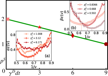
Figure 3: Schematic of the various critical exponents ($\nu$) and corresponding critical points ($\gamma^{K}_{c}$, $p^{K}_{c}$) obtained along the line ($9p^{S}+\gamma^{D}dt=18$) in the frame of total probability of measurements ($p^{S}=p^{K}+p^{D}$) versus effective density measurement strength ($\gamma^{D}dt$). The data for different system sizes is collected in two ways: (a) $\gamma^{D}dt$, $p^{K}=p^{D}=p^{S}/2$, and $\gamma^{K}dt$ are varied. (b) $\gamma^{D}dt=\gamma^{K}dt$, and $p^{K},\;p^{D}$ are varied by following the relation $p^{K}+p^{D}=p^{S}$. The other specific choice of parameters for different cases is as follows: ($\blacksquare$) $dt=0.05$, $\gamma^{D}=1$, $\alpha=14000$, ($\bigstar$) $dt=1$, $\alpha=2500$, $\beta=5000$, ($\Diamondblack$) $dt=1$, $\alpha=13000$, $\beta=2500$, ($\medbullet$) $dt=1$, $\beta=300$.

As a first step towards tracking the universal properties of the transition for generic coupling between system and detector, we consider the dynamics in the two previously studied limits of strong projective measurement ($\gamma dt\gg 1$, and $p^{K}+p^{D}=1$) and weak continuous monitoring ($\gamma dt\rightarrow 1$, and $p^{K}=p^{D}=1$). Fig. 2(a) shows the finite-size scaling analysis of the topological entanglement entropy as a function of the tunning parameter $\gamma^{K}/\gamma^{D}$ for the weak continuous limit.

The analysis is performed with small time steps $dt=0.05$; such that the effective strength of density measurement ($\gamma^{D}=1$) and Kitaev measurement ($\gamma^{K}$) is weak, i.e., $\gamma^{K,D}dt\to 0$. Thus, the back-action from the detector mirrors the Wiener process and results in stochastic Schrödinger dynamics in our controlled back-action setup. The inset of Figure 2(a) presents the scaling of TEE given in Eq. 9 at the critical point $\gamma^{K}/\gamma^{D}\approx 1.008$ for the critical exponent $\nu=5/3$.

To study the best fit to the scaling exponent, we examine the objective function $\epsilon(\nu)$ introduced in Ref.  [13]. This function is defined as the mean squared deviation of the topological entanglement entropy data for a fixed system size from their optimally fitted data, as detailed in Ref. [43]. The results are depicted as pink squares in Figure 3(a). We find that the critical exponent which minimized $\epsilon(\nu)$ is an agreement ($\gamma^{K}_{c}=\gamma^{D}$, $\nu=5/3$) with previous works on weak continuous monitoring of free fermionic chains [19].

Next, we examine the strong coupling case. In this limit, projectively measuring the state of the local detector is akin to performing a projective measurement on the system’s local degrees of freedom. The topological entanglement undergoes a phase transition at a critical probability value of $p^{K}_{c}=0.502$ in the system, as shown in Fig. 2(f). The corresponding data collapse onto a universal scaling function with critical exponent $\nu=4/3$ is shown as brown circles in the inset of Fig. 3(b). Another verification for the critical exponent is provided by the study of the objective function, showing a minimum at the critical exponent $\nu=4/3$ for a critical value $p_{c}^{K}=0.502$ as depicted in Fig. 3(b). This critical exponent value precisely matches the percolation prediction [13].

Having established that our methodology produced the correct scaling in the two limits, we next tackle the evolution of the universal behavior between them. For this purpose, we follow a line in the parameter space spanned by $p^{S}$ and $\gamma^{D}dt$, which connects the two limits, and examine the critical properties of the topological entanglement transition at intermediate points along the line, see Fig. 3. The strong projective limit is marked by the $\medbullet$ ($\gamma^{D}dt=9,p^{S}=1$), while the continuous limit is marked by a $\blacksquare$ ($\gamma^{D}dt=.05,p^{S}=2p^{K}=2p^{D}=2$).

We present the results of our study for two intermediate points marked by a $\bigstar$ ($p^{S}=1.667$, $\gamma^{D}dt=3$) and a $\Diamondblack$ ($p^{S}=1.333$, $\gamma^{D}dt=6$) on the line connecting the projective ($\medbullet$ ) and continuous ($\blacksquare$) limits in Fig. 3. For each point $(p^{S},\gamma^{D}dt)$ shown in Fig. 3 we tune across the transition in two ways:
(i) Fixing equal measurement probabilities $p^{D}=p^{K}=p^{S}/2$, while varying the relative measurement strength ($\gamma^{K}/\gamma^{D}$) .
(ii) Fixing equal measurement strength $\gamma^{K}=\gamma^{D}$ while varying the relative probabilities of the two measurements such that their sum is fixed, i.e. $p^{K}=p^{S}-p^{D}$.

The finite size scaling of the topological entanglement entropy (TEE) for the $\bigstar$ and for the $\Diamondblack$ in Fig. 3 are shown in Fig. 2 (b)-(c), and (d)-(e), respectively. Data collapses near the critical point are illustrated in the inset of the respective figures and confirmed by the objective function $\epsilon(\nu)$ in Fig. 3 (a,b) plotted for star and diamond markers. Remarkably, for each of the intermediate points ($\bigstar$, $\Diamondblack$), the same critical exponent is obtained when tunning across the transition using (i) the relative strength ($\gamma^{K}/\gamma^{D}$) as $\bigstar,\Diamondblack$, Fig. 3(a) or (ii) the relative probabilities $p^{K}=p^{S}-p^{D}$ as $\largestar,\Diamond$ in Fig. 3(b). It’s noteworthy that the critical exponent monotonously increases between the weak continuous ($\blacksquare$) and the projective ($\medbullet$) configurations.

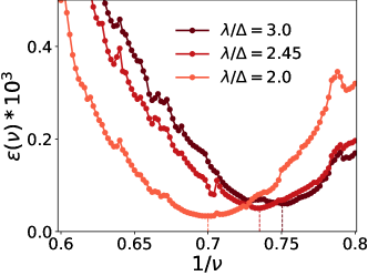
Figure 4: The objective function ($\epsilon(\nu)$) as a function of critical exponents ($\nu$) corresponding to different separations between two Gaussian distributions of the detector’s state ($2\lambda/\Delta$). Other parameter selections include: $dt=\Delta=1$, $\gamma^{D}=\gamma^{K}=4,6,9$, $\lambda=\sqrt{\gamma^{K}dt}=\sqrt{\gamma^{D}dt}$ and $p^{K}=1-p^{D}$ , considering various system sizes.

Finally, we study the stability of the percolation universality class to generic coupling between the system and detector. For this purpose, we study the correlation length critical exponent by perturbing around the strong coupling limit. In particular, we reduce the coupling strength $\lambda$, keeping the ratio between the two measurement rates $\gamma^{K}/\gamma^{D}$ and the sum of measurement probabilities $p^{s}$ fixed to $1$. This is equivalent to moving along the horizontal line passing through the point $\medbullet$ in Fig. 3, and corresponds to reducing the separation between the two Gaussian distributions ($\lambda/\Delta$). We find a significant change in the scaling exponent of the TEE phase transition, $\nu$, even in the regime $\lambda/\Delta>1$. This indicates that the projective limit is destabilized as the coupling between the system and detector is weakened. This is exemplified by the shift of the global minimum of the objective function for different values of $\lambda/\Delta$ in Fig. 4.

Discussion and conclusion - We developed a general methodology to study the dynamics driven by competing Gaussian measurements, with tunable coupling between the system and detector. This method continuously interpolates between projective measurement and weak continuous monitoring. In the strong projective limit, the dynamics can be mapped onto 2D percolation [13, 44, 45, 46, 47] and the critical properties are confirmed numerically. Meanwhile, weak non-projective measurements exhibit different universal behaviors [19]. Our work establishes a crucial link between these limits and allows to track the evolution of the universal properties of the topological entanglement transitions between these two limiting behaviors.

We find that the critical exponents that characterize the diverging correlation length at the transition grow monotonously as one moves away from the projective limit $\nu=4/3$ towards the weak continuous limit $\nu=5/3$. The monotonous increase in the correlation length $(p-p_{c})^{-\nu}$ with the reduced measurement strength can be understood from the percolation picture when perturbing around the strong projective limit. Here, measurements are mapped to cuts in the network [14]. When perturbing away from this limit by weakening the measurement strength, this would partially ”heal” a fraction of cuts in the grid, thus increasing the correlation length of a connected cluster. Our results indicate that the mapping to 2D classical percolation fails to describe the generic coupling between system and environment, even when that coupling is relatively strong.

Acknowledgments- We thank Graham Kells and Chun Y. Leung for their valuable discussions and time. A.R. acknowledges the support from the Royal Society, grant no. IECR2212041. We are grateful to the cluster facilities at Ben-Gurion University, Lancaster University, and Laboratoire de Physique des Solides CNRS, where large-scale calculations in this project were run. R. N. acknowledges the financial support of the Krietman fellowship at BGU and thanks the ICTP Visitors Program for hospitality. The authors would like to thank the Institut Henri Poincaré (UAR 839 CNRS-Sorbonne Université) and the LabEx CARMIN (ANR-10-LABX-59-01) for their support.

I Supplementary

II A. Objective Function $\epsilon(\nu)$

In order to investigate the most suitable scaling exponent, we analyze the objective function $\epsilon(\nu)$, which needs to be minimized to determine the precise critical exponent ($\nu$) corresponding to a critical point ($\gamma^{K}_{c}$ or $p^{K}_{c}$). This involves analyzing the behavior of the topological entanglement entropy $y=\bar{S}_{T}(q,L)$ as a function of $x=(q-q_{c})L^{1/\nu}$ for a fixed system size $L$, which aligns onto the curve $y=F(x)$ with the correct choice of $\nu$. Thus, the objective function $\epsilon(\nu)$ is expressed as:

$$\epsilon(\nu)=\frac{1}{n-2}\displaystyle\sum_{i=2}^{n-1}(y_{i}-\bar{y}_{i})^{2},$$ (10)

with $x_{i}=(q_{i}-q_{c})L_{i}^{1/\nu}$, $y_{i}=\bar{S}_{T}(q_{i},L)$. Additionally, $\bar{y}_{i}-y_{i+1}=\frac{y_{i+1}-y_{i-1}}{x_{i+1}-x_{i-1}}(x_{i}-x_{i+1})$ as the anticipated or optimal value of $y_{i}$. Here, $i$ encompasses all data points across various system sizes $L$ and variables $q=\gamma^{K}$ or $q=p^{K}$, arranged based on their $x$ values such that $x_{1}<x_{2}<\ldots<x_{n}$, with $n$ representing the total number of data points. The results of objective functions are discussed in Fig. 3 for different sets of parameters.

III B. Fitted Data

Here, we represent the fitted data of Fig. 2(a,c,e) and Fig. 3(a) for the same choice of parameters in Fig. 5.

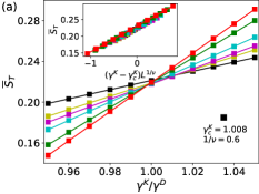
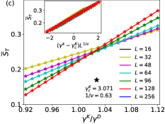
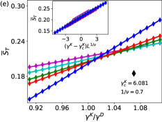
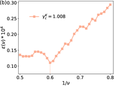
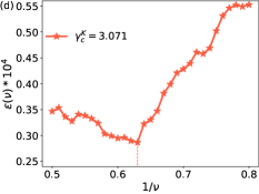
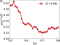
Figure 5: (a,c,e) The averaged topological entanglement entropy ($\bar{S}_{T}$) in units of $\log 2$ as a function of relative measurement strength ($\gamma^{K}/\gamma^{D}$) and fixed rate ($p^{K}=p^{D}=0.5p^{S}=1,0.833,0.667$) of the two measurements $\hat{M}^{K}$ and $\hat{M}^{D}$ for different system sizes. Below is the respective (b,d,f) objective function ($\epsilon(\nu)$) of this fitted data of Fig. 2(a,c,e). All the inset shows the scaling across the critical points ($\gamma^{K}_{c}$) with the corresponding scaling exponents ($\nu$). The details of different parameters are the same as Fig. 3(a,c,e), i.e., ($\blacksquare$) $\gamma^{D}=1$, $p^{D}=p^{K}=1$, ($\bigstar$) $\gamma^{D}=\gamma^{K}=3$, $p^{K}+p^{D}=1.667$, ($\Diamondblack$) $\gamma^{D}=\gamma^{K}=6$, $p^{K}+p^{D}=1.333$.

It is observed that the scaling exponents ($\nu$) and critical points ($\gamma^{K}_{c}$) follow a similar behavior as in Fig. 3(a), namely, the correlation length exponent $\nu$ decreases monotonically with the increase in measurement strengths.

IV C. Extra Data

In this section, we present the behavior of averaged topological entanglement entropy for a fixed system size $L=64$ with various measurement parameters.

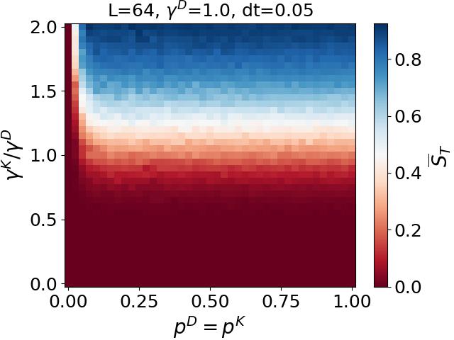
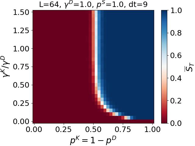
(a) (b) (c)

Figure 6: The averaged topological entanglement entropy ($\bar{S}_{T}$) for $L=64$ as a function of measurement strength ($\gamma^{K}$) and probability ($p^{D}$). The choice of parameters for different cases is as follows: (a) $\gamma^{D}=1$, $p^{D}=p^{K}$ with $dt=0.05$, (b) $\gamma^{D}=1$, $p^{K}+p_{D}=p^{S}=1$ with $dt=9$, (c) $\gamma^{D}=9$, $p^{K}=1$ with $dt=1$.

The choice of short time step $dt=0.05$ which leads to effective weak measurement strengths, i.e., $\sqrt{\gamma^{k,D}dt}<1$ in Fig. 6(a) signifies the weak continuous measurements. Here, the transition occurs across the relative measurement strength $\gamma^{K}/\gamma^{D}=1$ after a sufficient rate of probabilities. However, the selection of a time step $dt=9$ results in a strong measurement strength $\sqrt{\gamma^{k,D}dt}>1$, as illustrated in Fig. 6(b), indicating the strong projective limit. In this case, the transition across an equal rate of probabilities,i.e., $p^{K}=p^{D}$, remains the same after suitably strong measurement strengths roughly $\gamma^{K}dt=\gamma^{D}dt=9$. Figure 6(c) depicts a mixed scenario where phase transition happens at different Kitaev measurement strengths ($\gamma^{K}$) with a change in density-measurement rate $p^{D}$.

References

- Jacobs [2014] K. Jacobs, Quantum Measurement Theory and its Applications (Cambridge University Press, Cambridge, 2014).
- Zeng and Chen [2019] B. Zeng and X. Chen, Quantum information meets quantum matter, Quantum Science and Technology (Springer, New York, NY, 2019).
- Li et al. [2018] Y. Li, X. Chen, and M. P. A. Fisher, Quantum Zeno effect and the many-body entanglement transition, Phys. Rev. B 98, 205136 (2018).
- Fisher et al. [2023] M. P. Fisher, V. Khemani, A. Nahum, and S. Vijay, Random Quantum Circuits, Annual Review of Condensed Matter Physics 14, 335 (2023).
- Chan et al. [2019] A. Chan, R. M. Nandkishore, M. Pretko, and G. Smith, Unitary-projective entanglement dynamics, Phys. Rev. B 99, 224307 (2019).
- Skinner et al. [2019] B. Skinner, J. Ruhman, and A. Nahum, Measurement-Induced Phase Transitions in the Dynamics of Entanglement, Phys. Rev. X 9, 031009 (2019).
- Nahum et al. [2017] A. Nahum, J. Ruhman, S. Vijay, and J. Haah, Quantum entanglement growth under random unitary dynamics, Phys. Rev. X 7, 031016 (2017).
- Szyniszewski et al. [2019] M. Szyniszewski, A. Romito, and H. Schomerus, Entanglement transition from variable-strength weak measurements, Phys. Rev. B 100, 064204 (2019).
- Choi et al. [2020] S. Choi, Y. Bao, X.-L. Qi, and E. Altman, Quantum error correction in scrambling dynamics and measurement-induced phase transition, Phys. Rev. Lett. 125, 030505 (2020).
- goo [2023] Measurement-induced entanglement and teleportation on a noisy quantum processor, Nature 622, 481 (2023).
- Koh et al. [2023] J. M. Koh, S.-N. Sun, M. Motta, and A. J. Minnich, Measurement-induced entanglement phase transition on a superconducting quantum processor with mid-circuit readout, Nature Physics 19, 1314 (2023).
- Noel et al. [2022] C. Noel, P. Niroula, D. Zhu, A. Risinger, L. Egan, D. Biswas, M. Cetina, A. V. Gorshkov, M. J. Gullans, D. A. Huse, et al., Measurement-induced quantum phases realized in a trapped-ion quantum computer, Nature Physics 18, 760 (2022).
- Lavasani et al. [2021a] A. Lavasani, Y. Alavirad, and M. Barkeshli, Measurement-induced topological entanglement transitions in symmetric random quantum circuits, Nat. Phys. 17, 342 (2021a).
- Lavasani et al. [2021b] A. Lavasani, Y. Alavirad, and M. Barkeshli, Topological Order and Criticality in $(2+1)\mathrm{D}$ Monitored Random Quantum Circuits, Phys. Rev. Lett. 127, 235701 (2021b).
- Lang and Büchler [2020] N. Lang and H. P. Büchler, Entanglement transition in the projective transverse field Ising model, Phys. Rev. B 102, 094204 (2020).
- Ippoliti et al. [2021] M. Ippoliti, M. J. Gullans, S. Gopalakrishnan, D. A. Huse, and V. Khemani, Entanglement phase transitions in measurement-only dynamics, Phys. Rev. X 11, 011030 (2021).
- Sang and Hsieh [2021] S. Sang and T. H. Hsieh, Measurement-protected quantum phases, Phys. Rev. Research 3, 023200 (2021).
- Roy et al. [2020] S. Roy, J. T. Chalker, I. V. Gornyi, and Y. Gefen, Measurement-induced steering of quantum systems, Phys. Rev. Research 2, 033347 (2020).
- Kells et al. [2023] G. Kells, D. Meidan, and A. Romito, Topological transitions in weakly monitored free fermions, SciPost Phys. 14, 031 (2023).
- Kitaev [2003] A. Kitaev, Fault-tolerant quantum computation by anyons, Annals of Physics 303, 2 (2003).
- Kitaev [2006] A. Kitaev, Anyons in an exactly solved model and beyond, Annals of Physics January Special Issue, 321, 2 (2006).
- Klocke and Buchhold [2023] K. Klocke and M. Buchhold, Majorana loop models for measurement-only quantum circuits, Phys. Rev. X 13, 041028 (2023).
- Fava et al. [2023] M. Fava, L. Piroli, T. Swann, D. Bernard, and A. Nahum, Nonlinear sigma models for monitored dynamics of free fermions, Phys. Rev. X 13, 041045 (2023).
- Alberton et al. [2021] O. Alberton, M. Buchhold, and S. Diehl, Entanglement Transition in a Monitored Free-Fermion Chain: From Extended Criticality to Area Law, Phys. Rev. Lett. 126, 170602 (2021).
- Szyniszewski et al. [2020] M. Szyniszewski, A. Romito, and H. Schomerus, Universality of entanglement transitions from stroboscopic to continuous measurements, Phys. Rev. Lett. 125, 210602 (2020).
- Cao et al. [2019] X. Cao, A. Tilloy, and A. De Luca, Entanglement in a Fermion chain under continuous monitoring, SciPost Physics 7, 024 (2019).
- Brandt [1999] H. E. Brandt, Positive operator valued measure in quantum information processing, American Journal of Physics 67, 434 (1999).
- Wiseman and Milburn [2009] H. M. Wiseman and G. J. Milburn, Quantum Measurement and Control (Cambridge University Press, Cambridge, 2009).
- Barchielli and Gregoratti [2009] A. Barchielli and M. Gregoratti, Quantum Trajectories and Measurements in Continuous Time: The Diffusive Case, Lecture Notes in Physics, Vol. 782 (Springer, Berlin, Heidelberg, 2009).
- Szyniszewski et al. [2023] M. Szyniszewski, O. Lunt, and A. Pal, Disordered monitored free fermions, Phys. Rev. B 108, 165126 (2023).
- Merritt and Fidkowski [2023] J. Merritt and L. Fidkowski, Entanglement transitions with free fermions, Phys. Rev. B 107, 064303 (2023).
- Zeng and Zhou [2016] B. Zeng and D. L. Zhou, Topological and error-correcting properties for symmetry-protected topological order, EPL 113, 56001 (2016).
- Fromholz et al. [2020] P. Fromholz, G. Magnifico, V. Vitale, T. Mendes-Santos, and M. Dalmonte, Entanglement topological invariants for one-dimensional topological superconductors, Phys. Rev. B 101, 085136 (2020).
- Kitaev and Preskill [2006] A. Kitaev and J. Preskill, Topological Entanglement Entropy, Phys. Rev. Lett. 96, 110404 (2006).
- Levin and Wen [2006] M. Levin and X.-G. Wen, Detecting topological order in a ground state wave function, Phys. Rev. Lett. 96, 110405 (2006).
- Mondal et al. [2022] S. Mondal, S. Bandyopadhyay, S. Bhattacharjee, and A. Dutta, Detecting topological phase transitions through entanglement between disconnected partitions in a Kitaev chain with long-range interactions, Phys. Rev. B 105, 085106 (2022).
- Micallo et al. [2020] T. Micallo, V. Vitale, M. Dalmonte, and P. Fromholz, Topological entanglement properties of disconnected partitions in the Su-Schrieffer-Heeger model, SciPost Phys. Core 3, 012 (2020).
- Peschel [2003] I. Peschel, Calculation of reduced density matrices from correlation functions, J. Phys. A: Math. Gen. 36, L205 (2003).
- Peschel and Eisler [2009] I. Peschel and V. Eisler, Reduced density matrices and entanglement entropy in free lattice models, J. Phys. A: Math. Theor. 42, 504003 (2009).
- Keating and Mezzadri [2004] J. Keating and F. Mezzadri, Random Matrix Theory and Entanglement in Quantum Spin Chains, Commun. Math. Phys. 252, 543 (2004).
- Nehra et al. [2020] R. Nehra, D. S. Bhakuni, A. Ramachandran, and A. Sharma, Flat bands and entanglement in the Kitaev ladder, Phys. Rev. Res. 2, 013175 (2020).
- Eisert et al. [2010] J. Eisert, M. Cramer, and M. B. Plenio, Colloquium : Area laws for the entanglement entropy, Rev. Mod. Phys. 82, 277 (2010).
- [43] See Supplemental Material for (i) objective function, and (ii) Fitted data.
- Roósz et al. [2016] G. Roósz, R. Juhász, and F. Iglói, Nonequilibrium dynamics of the Ising chain in a fluctuating transverse field, Phys. Rev. B 93, 134305 (2016).
- Sykes and Essam [1964] M. F. Sykes and J. W. Essam, Exact Critical Percolation Probabilities for Site and Bond Problems in Two Dimensions, Journal of Mathematical Physics 5, 1117 (1964).
- Stauffer and Aharony [2018] D. Stauffer and A. Aharony, Introduction to percolation theory (CRC press, 2018).
- Deng and Yang [2006] Y. Deng and X. Yang, Finite-size scaling of energylike quantities in percolation, Phys. Rev. E 73, 066116 (2006).