On the addition of a large scalar multiplet to the Standard Model

Abstract

We consider the addition of a single $SU(2)$ multiplet of complex scalar fields to the Standard Model (SM). We explicitly consider the various possible values of the weak isospin $J$ of that multiplet, up to and including $J=7/2$. We allow the multiplet to have arbitrary weak hypercharge. The scalar fields of the multiplet are assumed to have no vacuum expectation value; the mass differences among the components of the multiplet originate in its coupling, present in the scalar potential (SP), to the Higgs doublet of the SM. We derive exact bounded-from-below and unitarity conditions on the SP, thereby constraining those mass differences. We compare those constraints to the ones that may be derived from the oblique parameters.

1 Introduction

In this paper, we study the model of New Physics (NP), i.e. of physics beyond the Standard Model (SM), wherein one adds to the SM one gauge-$SU(2)$ multiplet $\chi$ with weak isospin $J$ and consisting of $n=2J+1$ complex scalar fields. The multiplet has un-specified weak hypercharge $Y$; therefore, the model enjoys an accidental $U(1)$ symmetry wherein one rephases $\chi$ through an arbitrary phase. The scalar fields that compose $\chi$ are assumed not to have any vacuum expectation value (VEV), even if one of them—depending on $Y$ and $J$—may happen to be electrically neutral. There is in the scalar potential (SP) a renormalizable coupling

$$\lambda_{4}\,\sum_{a=1}^{3}\left(H^{\dagger}\,\frac{\tau_{a}}{2}\,H\right)\left[\chi^{\dagger}\,T_{a}^{(J)}\,\chi\right]$$ (1)

of $\chi$ to the Higgs doublet $H$ of the SM. In Eq. (1),

$\lambda_{4}$ is a dimensionless coefficient,

the $\tau_{a}$ are the Pauli matrices,

one conceives of $\chi$ as a column vector of $n$ scalar fields,

the $T_{a}^{(J)}$ are the $n\times n$ matrices that represent $su(2)$ in the $J$-isospin representation.

The coupling (1) generates, upon the neutral component of $H$ acquiring VEV $v$, a squared-mass difference $\Delta m^{2}\propto v^{2}$ between any two components of $\chi$ whose third component of isospin differs by one unit.

This NP model was firstly (to our knowledge) considered thirty years ago [1] as a paradigm for potentially large oblique parameters (OPs). It has later been studied as a model for “minimal” dark matter [2] and, more recently [3], as an explanation for the unexpectedly high value of the $W^{\pm}$ mass measured by the CDF-II Collaboration. Twelve years ago, Logan and her collaborators [4] have shown that $n$ cannot exceed eight, lest perturbative unitarity in the scattering of two scalars of $\chi$ to two $SU(2)$ gauge bosons be violated; they also derived mixed constraints on $J$ and $Y$. Logan’s work was revived and expanded very recently [5]. In another recent paper [6], the specific case of the addition of an $SU(2)$ scalar quadruplet to the SM has been considered; the hypercharge of that quadruplet has been restricted to the values $1/2$ or $3/2$, because in those two cases additional quartic couplings—beyond the one of Eq. (1)—of the types $\chi HHH$ and/or $\chi\chi\chi H$ may be present. (The accidental $U(1)$ symmetry then does not exist, because $Y$ has a well-defined value.) The case studied in Ref. [6] is on the one hand more restricted than the one in this paper, because $\chi$ has fixed $J=3/2$, but on the other hand it is more complicated, because additional quartic terms are allowed in the SP.

In this paper we want to constrain the modulus of the coefficient $\lambda_{4}$ of the term (1) of the SP; in so doing, we place an upper bound on $\Delta m^{2}$. We do this by considering both the unitarity (UNI) and the bounded-from-below (BFB) conditions on the quartic part of the SP. Remarkably, the upper bound on $\Delta m^{2}$ results from both the UNI and the BFB conditions, and not just from the former ones. We firstly show this fact, in a simplified version of the SP, in Section 2; later on, in Section 3, we consider the full SP. Section 4 contains the confrontation of our NP model with the OPs that it generates; we investigate whether the phenomenological OPs constrain $\Delta m^{2}$ more or less than the UNI/BFB conditions. Section 5 contains our conclusions. Appendix A explicitly lists the UNI conditions for all the values of $n$ through eight.

2 Potential without terms four-linear on $\chi$

In our model of NP there is the SM scalar doublet $H$ with hypercharge $1/2$ and an $SU(2)$ scalar multiplet $\chi$ with weak isospin $J$, which is a positive number, either integer or half-integer. The multiplet $\chi$ has

$$n=2J+1$$ (2)

components $\chi_{I}$ ($I=J,\ J-1,\ J-2,\ \ldots,\ 1-J,\ -J$). Its hypercharge $Y$ remains un-specified, i.e. arbitrary. Together with the charge-conjugate multiplets $\tilde{H}$ and $\tilde{\chi}$, we have the four multiplets

$$H=\left(\begin{array}[]{c}a\\ b\end{array}\right),\quad\tilde{H}=\left(\begin{array}[]{c}b^{*}\\ -a^{*}\end{array}\right),\quad\chi=\left(\begin{array}[]{c}\chi_{J}\\ \chi_{J-1}\\ \chi_{J-2}\\ \vdots\\ \chi_{1-J}\\ \chi_{-J}\end{array}\right),\quad\tilde{\chi}=\left(\begin{array}[]{c}\chi_{-J}^{\ast}\\ -\chi_{1-J}^{\ast}\\ \vdots\\ \left(-1\right)^{2J}\chi_{J-2}^{\ast}\\ -\left(-1\right)^{2J}\chi_{J-1}^{\ast}\\ \left(-1\right)^{2J}\chi_{J}^{\ast}\end{array}\right).$$ (3)

Here, $a$, $b$, and the $\chi_{I}$ are complex Klein–Gordon fields. Their third components of isospin are

$$a:\frac{1}{2},\quad b:-\frac{1}{2},\quad\chi_{I}:I,\quad\chi_{I}^{\ast}:-I.$$ (4)

When one multiplies $\chi$ by $\tilde{\chi}$ one obtains, among other $SU(2)$ representations, the singlet

$$F_{2}\equiv\left(\chi\otimes\tilde{\chi}\right)_{\mathbf{1}}=\sum_{I=-J}^{J}\left|\chi_{I}\right|^{2}$$ (5)

and the triplet

$$\left(\chi\otimes\tilde{\chi}\right)_{\mathbf{3}}=\left(\begin{array}[]{c}\displaystyle{-\sum_{I=1-J}^{J}\sqrt{\frac{J^{2}-I^{2}+J+I}{2}}\ \chi_{I}\,\chi_{I-1}^{\ast}}\\[5.69054pt] \displaystyle{\sum_{I=-J}^{J}I\left|\chi_{I}\right|^{2}}\\[5.69054pt] \displaystyle{\sum_{I=1-J}^{J}\sqrt{\frac{J^{2}-I^{2}+J+I}{2}}\ \chi_{I}^{\ast}\,\chi_{I-1}}\end{array}\right).$$ (6)

Applying the general Eq. (6) to the specific case of $H$ (i.e., using $J=1/2$, $\chi_{1/2}=a$, and $\chi_{-1/2}=b$), we obtain

$$\left(H\otimes\tilde{H}\right)_{\mathbf{3}}=\left(\begin{array}[]{c}\displaystyle{-\frac{ab^{\ast}}{\sqrt{2}}}\\[5.69054pt] \displaystyle{\frac{\left|a\right|^{2}-\left|b\right|^{2}}{2}}\\[5.69054pt] \displaystyle{\frac{a^{\ast}b}{\sqrt{2}}}\end{array}\right).$$ (7)

The scalar potential $V$ has a quadratic part $V_{2}$ and a quartic part $V_{4}$:

$$V=V_{2}+V_{4}.$$ (8)

Obviously,

$$V_{2}=-\mu_{1}^{2}F_{1}+\mu_{2}^{2}F_{2},$$ (9)

where

$$F_{1}\equiv\left(H\otimes\tilde{H}\right)_{\mathbf{1}}=\left|a\right|^{2}+\left|b\right|^{2}$$ (10)

and $F_{2}$ is defined in Eq. (5). We assume both coefficients $\mu_{1}^{2}$ and $\mu_{2}^{2}$ to be positive, so that $H$ has VEV $\left\langle 0\left|b\right|0\right\rangle=v$ but $\chi$ does not have VEV.

The quartic part of the potential contains

• the term $\left[\left(H\otimes\tilde{H}\right)_{\mathbf{1}}\right]^{2}$, with coefficient $\displaystyle{\frac{\lambda_{1}}{2}}$;

• the term $\left(H\otimes\tilde{H}\right)_{\mathbf{1}}\,\left(\chi\otimes\tilde{\chi}\right)_{\mathbf{1}}$, with coefficient $\lambda_{3}$;

• the term $\left[\left(H\otimes\tilde{H}\right)_{\mathbf{3}}\otimes\left(\chi\otimes\tilde{\chi}\right)_{\mathbf{3}}\right]_{\mathbf{1}}$, with coefficient $\lambda_{4}$;

• various terms that are four-linear in the components of $\chi$. We keep those terms un-specified in this section.

Thus,

$$V_{4}=\frac{\lambda_{1}}{2}\,F_{1}^{2}+\lambda_{3}F_{1}F_{2}+\lambda_{4}F_{4}+\mbox{terms\ four-linear\ in\ the}\ \chi_{I},$$ (11)

where

$$F_{4}\equiv\frac{\left|a\right|^{2}-\left|b\right|^{2}}{2}\,\sum_{I=-J}^{J}I\left|\chi_{I}\right|^{2}+\frac{z+z^{\ast}}{2}.$$ (12)

We have defined

$$z\equiv ab^{\ast}\sum_{I=1-J}^{J}\chi_{I}^{\ast}\,\chi_{I-1}\sqrt{J^{2}-I^{2}+J+I}.$$ (13)

From Eqs. (8), (9), (11), and (12) the mass-squared of the scalar $\chi_{I}$ is

$$m_{I}^{2}=\mu_{2}^{2}+\left(\lambda_{3}-\frac{\lambda_{4}}{2}\,I\right)\left|v\right|^{2}.$$ (14)

This implies that the difference between the masses-squared of $\chi_{I}$ and $\chi_{I+1}$ is

$$\Delta m^{2}=\frac{\left|\lambda_{4}v^{2}\right|}{2},$$ (15)

which is $I$-independent. An upper bound on $\left|\lambda_{4}\right|$ is therefore equivalent to an upper bound on $\Delta m^{2}$.

The VEV of $V$ is

$$\left\langle 0\left|V\right|0\right\rangle=-\mu_{1}^{2}v^{2}+\frac{\lambda_{1}}{2}\,v^{4}.$$ (16)

Therefore, $\mu_{1}^{2}=\lambda_{1}v^{2}$. The mass-squared of the Higgs particle is $m_{H}^{2}=2\lambda_{1}v^{2}$. Since experimentally $m_{H}\approx$ 125 GeV and $v\approx$ 174 GeV, one has

$$\lambda_{1}\approx 0.258.$$ (17)

From now on we shall assume Eq. (17) to hold. Contrary to $\lambda_{1}$, the couplings $\lambda_{3}$ and $\lambda_{4}$ are free, but they are constrained by both the UNI and BFB conditions. We next derive those constraints.

2.1 Unitarity (UNI) conditions

Firstly suppose that $J$ is half-integer.

We consider the scattering of the two two-field states with hypercharge $Y+1/2$ and null third component of isospin, viz. of $\chi_{-1/2}a$ and $\chi_{1/2}b$. Their scattering matrix is

$$\left(\begin{array}[]{cc}\lambda_{3}-\lambda_{4}/4&\left(2J+1\right)\lambda_{4}/4\\ \left(2J+1\right)\lambda_{4}/4&\lambda_{3}-\lambda_{4}/4\end{array}\right).$$ (18)

The eigenvalues of this matrix are

$$\lambda_{3}+\frac{J\lambda_{4}}{2},\quad\lambda_{3}-\frac{\left(J+1\right)\lambda_{4}}{2}.$$ (19)

We next consider the scattering of the states with hypercharge $Y-1/2$ and null third component of isospin, viz. of $\chi_{-1/2}b^{\ast}$ and $\chi_{1/2}a^{\ast}$. Their scattering matrix is

$$\left(\begin{array}[]{cc}\lambda_{3}+\lambda_{4}/4&\left(2J+1\right)\lambda_{4}/4\\ \left(2J+1\right)\lambda_{4}/4&\lambda_{3}+\lambda_{4}/4\end{array}\right).$$ (20)

The eigenvalues of this matrix are

$$\lambda_{3}+\frac{\left(J+1\right)\lambda_{4}}{2},\quad\lambda_{3}-\frac{J\lambda_{4}}{2}.$$ (21)

Let secondly suppose that $J$ is an integer instead.

We consider the scattering of the two two-particle states with hypercharge $Y+1/2$ and third component of isospin $1/2$, viz. of $\chi_{0}a$ and $\chi_{1}b$. Their scattering matrix is

$$\left(\begin{array}[]{cc}\lambda_{3}&\left.\sqrt{J\left(J+1\right)}\,\lambda_{4}\right/2\\ \left.\sqrt{J\left(J+1\right)}\,\lambda_{4}\right/2&\lambda_{3}-\lambda_{4}/2\end{array}\right).$$ (22)

The eigenvalues of this matrix are the ones in Eq. (19).

We next consider the scattering of the states with hypercharge $Y-1/2$ and third component of isospin $1/2$, viz. of the states $\chi_{1}a^{\ast}$ and $\chi_{0}b^{\ast}$. Their scattering matrix is

$$\left(\begin{array}[]{cc}\lambda_{3}+\lambda_{4}/2&\left.\sqrt{J\left(J+1\right)}\,\lambda_{4}\right/2\\ \left.\sqrt{J\left(J+1\right)}\,\lambda_{4}\right/2&\lambda_{3}\end{array}\right).$$ (23)

The eigenvalues of this matrix are in Eq. (21).

Thus, the eigenvalues of the scattering matrices are the same, no matter whether $J$ is integer or half-integer.

We now impose the conditions that the moduli of all the eigenvalues in Eqs. (19) and (21) should be smaller than

$$M=8\pi.$$ (24)

We obtain

$$\left|\lambda_{3}\right|+\frac{J}{2}\left|\lambda_{4}\right| < M,$$ (25a)

$$\left|\lambda_{3}\right|+\frac{J+1}{2}\left|\lambda_{4}\right| < M.$$ (25b)

Condition (25b) is of course stronger than condition (25a), therefore one may neglect the latter.

The dispersion of the $2+n$ states that have zero third component of isospin and zero hypercharge, viz. of $\left|a\right|^{2}$, $\left|b\right|^{2}$, and the $n$ states $\left|\chi_{I}\right|^{2}$, produces the scattering matrix

$$\mathcal{S}=\left(\begin{array}[]{ccccc}2\lambda_{1}&\lambda_{1}&\lambda_{3}+\left.J\lambda_{4}\right/2&\cdots&\lambda_{3}-\left.J\lambda_{4}\right/2\\ \lambda_{1}&2\lambda_{1}&\lambda_{3}-\left.J\lambda_{4}\right/2&\cdots&\lambda_{3}+\left.J\lambda_{4}\right/2\\ \lambda_{3}+\left.J\lambda_{4}\right/2&\lambda_{3}-\left.J\lambda_{4}\right/2&0&\cdots&0\\ \vdots&\vdots&\vdots&\ddots&\vdots\\ \lambda_{3}-\left.J\lambda_{4}\right/2&\lambda_{3}+\left.J\lambda_{4}\right/2&0&\cdots&0\end{array}\right).$$ (26)

(The null sub-matrix in the lower right-hand corner of $\mathcal{S}$ occurs because we have neglected the terms in $V_{4}$ that are four-linear in the $\chi_{I}$. We shall remedy this neglect in the next section.) Computing $O^{T}\mathcal{S}O$, where

$$O=\frac{1}{\sqrt{2}}\left(\begin{array}[]{ccc}1&1&0\\ -1&1&0\\ 0&0&\sqrt{2}\end{array}\right),$$ (27)

one obtains the two matrices

$$\left(\begin{array}[]{cccc}\lambda_{1}&\left.J\,\lambda_{4}\right/\sqrt{2}&\cdots&-\left.J\,\lambda_{4}\right/\sqrt{2}\\ \left.J\,\lambda_{4}\right/\sqrt{2}&0&\cdots&0\\ \vdots&\vdots&\ddots&\vdots\\ -\left.J\,\lambda_{4}\right/\sqrt{2}&0&\cdots&0\end{array}\right),\quad\left(\begin{array}[]{cccc}3\lambda_{1}&\sqrt{2}\,\lambda_{3}&\cdots&\sqrt{2}\,\lambda_{3}\\ \sqrt{2}\,\lambda_{3}&0&\cdots&0\\ \vdots&\vdots&\ddots&\vdots\\ \sqrt{2}\,\lambda_{3}&0&\cdots&0\end{array}\right).$$ (28)

Computing the eigenvalues of these two matrices and setting their moduli to be smaller than $M$, we find

$$\left|\lambda_{1}\right|+\sqrt{\lambda_{1}^{2}+2\sum_{I=-J}^{J}I^{2}\lambda_{4}^{2}} < 2M,$$ (29a)

$$3\left|\lambda_{1}\right|+\sqrt{9\lambda_{1}^{2}+8\sum_{I=-J}^{J}\lambda_{3}^{2}} < 2M.$$ (29b)

Performing the sums over $I$ with the help of

$$\sum_{I=-J}^{J}\,1 = 2J+1,$$ (30a)

$$\sum_{I=-J}^{J}\,I^{2} = \frac{J\left(J+1\right)\left(2J+1\right)}{3},$$ (30b)

we obtain

$$\left|\lambda_{1}\right|+\sqrt{\lambda_{1}^{2}+\frac{2}{3}\,J\left(J+1\right)\left(2J+1\right)\lambda_{4}^{2}} < 2M,$$ (31a)

$$3\left|\lambda_{1}\right|+\sqrt{9\lambda_{1}^{2}+8\left(2J+1\right)\lambda_{3}^{2}} < 2M.$$ (31b)

The potential $V_{4}$ produces many other scatterings of two-particle states, but they all lead to UNI conditions that either repeat Eq. (25b), or repeat Eq. (31a), or repeat Eq. (31b), or are weaker than one of them.

2.2 Bounded-from-below (BFB) conditions

In order to evaluate the BFB conditions on $V_{4}$, it is handy to use the gauge wherein $b=0$. We use

$$\left|\sum_{I=-J}^{J}I\left|\chi_{I}\right|^{2}\right| = \left|J\left|\chi_{J}\right|^{2}+\left(J-1\right)\left|\chi_{J-1}\right|^{2}+\cdots-J\left|\chi_{-J}\right|^{2}\right|$$ (32a)

$$\leq JF_{2}$$ (32b)

to write, in that gauge,

$$V_{4}\geq\frac{\lambda_{1}}{2}\left|a\right|^{4}+\left(\lambda_{3}-\left.J\left|\lambda_{4}\right|\right/2\right)\left|a\right|^{2}F_{2}+\mbox{terms\ four-linear\ in\ the}\ \chi_{I}.$$ (33)

Since both $\left|a\right|^{2}\geq 0$ and $F_{2}\geq 0$, the conditions for $\left(\lambda_{1}/2\right)\left|a\right|^{4}+\left(\lambda_{3}-\left.J\left|\lambda_{4}\right|\right/2\right)\left|a\right|^{2}F_{2}$ to be non-negative, whatever the (non-negative) values of $\left|a\right|^{2}$ and $F_{2}$, are [9]

$$\lambda_{1} \geq 0,$$ (34a)

$$\lambda_{3} \geq 0,$$ (34b)

$$\left|\lambda_{4}\right| \leq \frac{2\lambda_{3}}{J}.$$ (34c)

Conditions (34) are necessary and sufficient for $V_{4}$ to be non-negative for arbitrary values of the fields $a$ and $\chi_{I}$. Since a gauge with $b=0$ can always be obtained, those conditions also hold for $V_{4}$ with arbitrary values of $a$, $b$, and the $\chi_{I}$.

2.3 Results

Transforming all the six relevant UNI and BFB conditions into strict equalities, we have

$$\lambda_{3}+\frac{J+1}{2}\left|\lambda_{4}\right| = M,$$ (35a)

$$\lambda_{1}+\sqrt{\lambda_{1}^{2}+\frac{2J\left(2J^{2}+3J+1\right)\lambda_{4}^{2}}{3}} = 2M,$$ (35b)

$$3\lambda_{1}+\sqrt{9\lambda_{1}^{2}+8\left(2J+1\right)\lambda_{3}^{2}} = 2M,$$ (35c)

$$\left|\lambda_{4}\right| = \frac{2}{J}\,\lambda_{3},$$ (35d)

where we have taken into account that both $\lambda_{1}$ and $\lambda_{3}$ are non-negative, cf. Eqs. (17) and (34b), respectively. Equation (35b) gives solution I:

$$\left|\lambda_{4}\right|=\sqrt{\frac{6M\left(M-\lambda_{1}\right)}{J\left(2J^{2}+3J+1\right)}}.$$ (36)

Equations (35a) and (35c) together produce solution II:

$$\left|\lambda_{4}\right| = \displaystyle{\frac{2M}{J+1}-\frac{\sqrt{2M\left(M-3\lambda_{1}\right)}}{\left(J+1\right)\sqrt{2J+1}},}$$ (37a)

$$\lambda_{3} = \displaystyle{\sqrt{\frac{M\left(M-3\lambda_{1}\right)}{2\left(2J+1\right)}}.}$$ (37b)

Equations (35a) and (35d) together lead to solution III:

$$\left|\lambda_{4}\right| = \displaystyle{\frac{2M}{2J+1},}$$ (38a)

$$\lambda_{3} = \displaystyle{\frac{J}{2J+1}\,M.}$$ (38b)

Equations (35c) and (35d) together give solution IV:

$$\left|\lambda_{4}\right|=\displaystyle{\frac{\sqrt{2M\left(M-3\lambda_{1}\right)}}{J\sqrt{2J+1}}}$$ (39)

and Eq. (37b), which is the solution of Eq. (35c).

Solutions I, II, III, and IV for $\left|\lambda_{4}\right|$ and $\lambda_{3}$ are plotted in Fig. 1.

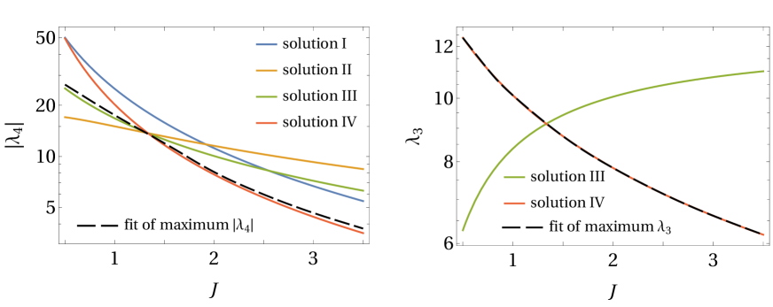
Figure 1: The solutions (36)–(39) for $\left|\lambda_{4}\right|$ (left panel) and $\lambda_{3}$ (right panel) versus $J$. We have used $M=8\pi$. The black dashed lines display the maximum allowed values of $\left|\lambda_{4}\right|$ and $\lambda_{3}$ described in subsection 3.3.

Notice that solutions II, III, and IV coincide when

$$2J+1=\frac{2MJ^{2}}{M-3\lambda_{1}},$$ (40)

i.e. when $J\approx 1.37$. When $J$ is larger than this value, i.e. when $\chi$ is either a quadruplet or a larger multiplet of $SU(2)$, then solution IV—which arises from both the UNI condition (31b) and the BFB condition (34c)—gives the strongest upper bound on both $\lambda_{3}$ and $\left|\lambda_{4}\right|$. Thus, both $\lambda_{3}$ and $\left|\lambda_{4}\right|$ are bounded from above by the interplay of a UNI condition and a BFB condition, for most possible values of $J$.

We remind the reader that, according to Eq. (34b), the minimum value of $\lambda_{3}$ is 0.

3 Full potential

The product $\chi\otimes\chi$ of two identical multiplets of $SU(2)$ only has a symmetric component—the anti-symmetric component vanishes because the two multiplets are equal—which consists of

$$t=\frac{1}{2}\,\mathrm{ceil}\left(n,2\right)$$ (41)

multiplets of $SU(2)$

$$\left(\chi\otimes\chi\right)_{\mathrm{symmetric}}=c\oplus d\oplus e\oplus\cdots\oplus q,$$ (42)

where

$c$ is an $SU(2)$ multiplet with weak isospin $2J$,

$d$ is an $SU(2)$ multiplet with weak isospin $2J-2$,

$e$ is an $SU(2)$ multiplet with weak isospin $2J-4$,

and so on; lastly, $q$ is either a triplet of $SU(2)$ if $J$ is half-integer, or $SU(2)$-invariant if $J$ is integer. Thus,

$$\left(\chi\otimes\chi\right)_{\mathrm{symmetric}}=\left(\begin{array}[]{c}c_{2J}\\ c_{2J-1}\\ \vdots\\ c_{-2J}\end{array}\right)\oplus\left(\begin{array}[]{c}d_{2J-2}\\ d_{2J-3}\\ \vdots\\ d_{2-2J}\end{array}\right)\oplus\left(\begin{array}[]{c}e_{2J-4}\\ e_{2J-5}\\ \vdots\\ e_{4-2J}\end{array}\right)\oplus\cdots,$$ (43)

where the sub-indices give the third component of isospin. The two-field states in each multiplet in the right-hand side of Eq. (43) are evaluated by using Clebsch–Gordan coefficients in the standard fashion. Thus,

$$c_{I} = \sum_{I^{\prime}=-J}^{J}\,\sum_{I^{\prime\prime}=-J}^{J}\,\delta_{I,I^{\prime}+I^{\prime\prime}}\left[\begin{array}[]{ccc}J&J&2J\\ I^{\prime}&I^{\prime\prime}&I\end{array}\right]\chi_{I^{\prime}}\chi_{I^{\prime\prime}},$$ (44c)

$$d_{I} = \sum_{I^{\prime}=-J}^{J}\,\sum_{I^{\prime\prime}=-J}^{J}\,\delta_{I,I^{\prime}+I^{\prime\prime}}\left[\begin{array}[]{ccc}J&J&2J-2\\ I^{\prime}&I^{\prime\prime}&I\end{array}\right]\chi_{I^{\prime}}\chi_{I^{\prime\prime}},$$ (44f)

$$e_{I} = \sum_{I^{\prime}=-J}^{J}\,\sum_{I^{\prime\prime}=-J}^{J}\,\delta_{I,I^{\prime}+I^{\prime\prime}}\left[\begin{array}[]{ccc}J&J&2J-4\\ I^{\prime}&I^{\prime\prime}&I\end{array}\right]\chi_{I^{\prime}}\chi_{I^{\prime\prime}},$$ (44i)

and so on.

The “terms four-linear in the $\chi_{I}$” in Eq. (11) are

a term $\displaystyle{\frac{\lambda_{2}}{2}\,F_{2}^{2}}$, where $F_{2}$ has been defined in Eq. (5);

a term $\lambda_{5}F_{5}$, where

$$F_{5}\equiv\sum_{I=2-2J}^{2J-2}\left|d_{I}\right|^{2};$$ (45)

a term $\lambda_{6}F_{6}$, where

$$F_{6}\equiv\sum_{I=4-2J}^{2J-4}\left|e_{I}\right|^{2};$$ (46)

and other analogous terms, up to $\lambda_{t+3}F_{t+3}$, where

$$F_{t+3}\equiv\left\{\begin{array}[]{lcl}\left|q_{1}\right|^{2}+\left|q_{0}\right|^{2}+\left|q_{-1}\right|^{2}&\Leftarrow&\mbox{half-integer}\ J,\\[2.84526pt] \left|q_{0}\right|^{2}.&\Leftarrow&\mathrm{integer}\ J.\end{array}\right.$$ (47)

The quartic part of the scalar potential thus is

$$V_{4}=\frac{\lambda_{1}}{2}\,F_{1}^{2}+\frac{\lambda_{2}}{2}\,F_{2}^{2}+\lambda_{3}F_{1}F_{2}+\lambda_{4}F_{4}+\sum_{i=5}^{t+3}\lambda_{i}F_{i}.$$ (48)

A term with the invariant

$$F_{3}\equiv\sum_{I=-2J}^{2J}\left|c_{I}\right|^{2}$$ (49)

has not been included in $V_{4}$ because $F_{3}$ linearly depends on the other invariants. Indeed,

$$F_{3}+\sum_{i=5}^{t+3}F_{i}=F_{2}^{2}.$$ (50)

3.1 BFB conditions

Let us consider again $\left(\chi\otimes\tilde{\chi}\right)_{\mathbf{3}}$ given in Eq. (6). The $SU(2)$-invariant quantity

$$\left|\left(\chi\otimes\tilde{\chi}\right)_{\mathbf{3}}\right|^{2}\equiv\left(\sum_{I=-J}^{J}I\left|\chi_{I}\right|^{2}\right)^{2}+\left|\sum_{I=1-J}^{J}\chi_{I}^{\ast}\chi_{I-1}\sqrt{J^{2}-I^{2}+J+I}\right|^{2}$$ (51)

is four-linear in the $\chi_{I}$ and therefore it must be linearly dependent on $F_{2}^{2}$ and the $F_{i}$. Indeed, one finds that

$$\left|\left(\chi\otimes\tilde{\chi}\right)_{\mathbf{3}}\right|^{2}=J^{2}F_{2}^{2}-\sum_{i=5}^{t+3}\kappa_{i}F_{i},$$ (52)

where the numbers $\kappa_{i}$ are given by

$$\kappa_{i}=\left(i-4\right)\left(4J+9-2i\right).$$ (53)

Notice that all the $\kappa_{i}$ are positive. We have explicitly checked, up to $J=10$, that Eqs. (52) and (53) are correct.

From Eq. (52),

$$\sum_{i=5}^{t+3}\kappa_{i}F_{i}-J^{2}F_{2}^{2}=-\left(\sum_{I=-J}^{J}I\left|\chi_{I}\right|^{2}\right)^{2}-\left|\frac{z}{ab}\right|^{2},$$ (54)

where $z$ has been defined in Eq. (13); hence, from the definition of $F_{4}$ in Eq. (12),

$$\sum_{i=5}^{t+3}\kappa_{i}F_{i}-J^{2}F_{2}^{2}=-\left(\frac{2F_{4}-z-z^{\ast}}{\left|a\right|^{2}-\left|b\right|^{2}}\right)^{2}-\left|\frac{z}{ab}\right|^{2}.$$ (55)

Therefore,

$$\sum_{i=5}^{t+3}\kappa_{i}F_{i}-J^{2}F_{2}^{2}+\frac{4F_{4}^{2}}{F_{1}^{2}} = \frac{1}{4\left|ab\right|^{2}\left(\left|a\right|^{4}-\left|b\right|^{4}\right)^{2}}\left\{\vphantom{\left[8\left|ab\right|^{2}F_{4}-\left(\left|a\right|^{2}+\left|b\right|^{2}\right)^{2}\left(z+z^{\ast}\right)\right]^{2}}\left(\left|a\right|^{4}-\left|b\right|^{4}\right)^{2}\left(z-z^{\ast}\right)^{2}\right.$$ (56)

$$\left.-\left[8\left|ab\right|^{2}F_{4}-\left(\left|a\right|^{2}+\left|b\right|^{2}\right)^{2}\left(z+z^{\ast}\right)\right]^{2}\right\}.$$

Thus,

$$\sum_{i=5}^{t+3}\kappa_{i}F_{i}-J^{2}F_{2}^{2}+\frac{4F_{4}^{2}}{F_{1}^{2}}\leq 0.$$ (57)

We now define the dimensionless quantities [10]

$$r \equiv \frac{F_{1}}{F_{2}},$$ (58a)

$$\gamma_{i} \equiv \frac{F_{i}}{F_{2}^{2}}\quad(i=5,\ldots,t+3),$$ (58b)

$$\delta \equiv \frac{2F_{4}}{JF_{1}F_{2}}.$$ (58c)

We then have, from Eq. (48),

$$\frac{V_{4}}{F_{2}^{2}} = \frac{\lambda_{1}}{2}\,r^{2}+\frac{\lambda_{2}}{2}+\lambda_{3}r+\frac{J}{2}\,\lambda_{4}r\delta+\sum_{i=5}^{t+3}\lambda_{i}\gamma_{i}$$ (59a)

$$= \frac{1}{2}\left(\begin{array}[]{cc}r,&1\end{array}\right)\left(\begin{array}[]{cc}\lambda_{1}&\lambda_{3}+\displaystyle{\frac{J}{2}\,\lambda_{4}\delta}\\[8.53581pt] \lambda_{3}+\displaystyle{\frac{J}{2}\,\lambda_{4}\delta}&\displaystyle{\lambda_{2}+2\sum_{i=5}^{t+3}\lambda_{i}\gamma_{i}}\end{array}\right)\left(\begin{array}[]{c}r\\ 1\end{array}\right).$$ (59g)

It follows from the definitions of $F_{2}$ and $F_{1}$ in Eqs. (5) and (10), respectively, that $r\geq 0$. Therefore, the conditions for $V_{4}\left/F_{2}^{2}\right.$ in Eq. (59g) to be non-negative are [9]

$$\lambda_{1} \geq 0,$$ (60a)

$$\lambda_{2}+2\,\sum_{i=5}^{t+3}\lambda_{i}\gamma_{i} \geq 0,$$ (60b)

$$\lambda_{3}+\frac{J}{2}\,\lambda_{4}\delta \geq -\sqrt{\lambda_{1}\left(\lambda_{2}+2\,\sum_{i=5}^{t+3}\lambda_{i}\gamma_{i}\right)}.$$ (60c)

The conditions (60b) and (60c) must hold for all possible values of $\delta$ and of the $\gamma_{i}$. It follows from the definitions of the $F_{i}$, cf. Eqs. (45) and (46), that the $\gamma_{i}\geq 0$. From Eq. (57),

$$\sum_{i=5}^{t+3}\kappa_{i}\gamma_{i}-J^{2}\left(1-\delta^{2}\right)\leq 0.$$ (61)

Thus, since all the $\kappa_{i}$ and the $\gamma_{i}$ are positive,

$$0\leq\sum_{i=5}^{t+3}\kappa_{i}\gamma_{i}\leq J^{2}\left(1-\delta^{2}\right),$$ (62)

and therefore $-1\leq\delta\leq+1$. It is advantageous to define

$$x=\frac{1+\delta}{2}\in\left[0,1\right].$$ (63)

Then Eq. (62) reads

$$0\leq\sum_{i=5}^{t+3}\kappa_{i}\gamma_{i}\leq 4J^{2}x\left(1-x\right).$$ (64)

This condition determines the domain of the $\gamma_{i}$, which has corners at the points [10]

$$\gamma_{5}=\cdots=\gamma_{t+3}=0,$$ (65a)

$$\gamma_{5}=\cdots=\gamma_{t+2}=0, \gamma_{t+3}=\frac{J^{2}}{\kappa_{t+3}},$$ (65b)

$$\gamma_{5}=\cdots=\gamma_{t+1}=\gamma_{t+3}=0, \gamma_{t+2}=\frac{J^{2}}{\kappa_{t+2}},$$ (65c)

$$\vdots \vdots$$

$$\gamma_{6}=\cdots=\gamma_{t+3}=0, \gamma_{5}=\frac{J^{2}}{\kappa_{5}}.$$ (65d)

Since $\lambda_{2}+2\sum_{i=5}^{t+3}\lambda_{i}\gamma_{i}$ is a linear function of the $\gamma_{i}$, condition (60b) just has to hold at the corners of the domain of the $\gamma_{i}$ in order to hold in the whole domain. We thus obtain necessary BFB conditions:

$$\lambda_{2} \geq 0,$$ (66a)

$$\widehat{\lambda}_{i} \geq 0,$$ (66b)

where

$$\widehat{\lambda}_{i} \equiv \lambda_{2}+q_{i},$$ (67a)

$$q_{i} \equiv \frac{2J^{2}}{\kappa_{i}}\,\lambda_{i}.$$ (67b)

Furthermore, condition (60c) must certainly hold at the point (65a) and for both $\delta=0$ and $\delta=\pm 1$. Therefore,

$$\lambda_{3} \geq -\sqrt{\lambda_{1}\lambda_{2}},$$ (68a)

$$\left|\lambda_{4}\right| \leq \frac{2}{J}\left(\lambda_{3}+\sqrt{\lambda_{1}\lambda_{2}}\right).$$ (68b)

The necessary BFB conditions (68a) and (68b) generalize conditions (34b) and (34c), respectively, when $\lambda_{2}$ is nonzero.

Condition (60c) must also hold at all the other corners (65) of the $\gamma_{i}$ domain. Therefore,

$$\lambda_{3}-\frac{J}{2}\,\lambda_{4}+J\lambda_{4}x\geq-\sqrt{\lambda_{1}\left[\lambda_{2}+4q_{i}x\left(1-x\right)\right]}$$ (69)

must hold for all $i=5,\ldots,t+3$ and for all $x\equiv\left[0,1\right]$. Thus, the functions

$$f_{i}\left(x\right)\equiv\lambda_{3}-\frac{J}{2}\,\lambda_{4}+J\lambda_{4}x+\sqrt{\lambda_{1}\left[\lambda_{2}+4q_{i}\left(x-x^{2}\right)\right]}\quad(i=5,\ldots,t+3)$$ (70)

must be non-negative $\forall x\in\left[0,1\right]$. Clearly [10],

$$\frac{\mathrm{d}f_{i}}{\mathrm{d}x} = J\lambda_{4}+\frac{2\sqrt{\lambda_{1}}\,q_{i}\left(1-2x\right)}{\sqrt{\lambda_{2}+4q_{i}\left(x-x^{2}\right)}},$$ (71a)

$$\frac{\mathrm{d}^{2}f_{i}}{\mathrm{d}x^{2}} = \frac{-4q_{i}\widehat{\lambda}_{i}\sqrt{\lambda_{1}}}{\left[\sqrt{\lambda_{2}+4q_{i}\left(x-x^{2}\right)}\right]^{3}}.$$ (71b)

Because of Eq. (66b), the second derivative of $f_{i}$ has sign opposite to the one of $q_{i}$, i.e. opposite to the one of $\lambda_{i}$. Since we have already ascertained—through condition (68b)—that both $f_{i}\left(0\right)\geq 0$ and $f_{i}\left(1\right)\geq 0$, the condition $f_{i}\left(x\right)\geq 0,\ \forall x\in\left[0,1\right]$ is equivalent to the following:

either $\mathrm{d}^{2}f_{i}\left/\mathrm{d}x^{2}\right.<0$,

or there is no real number $x_{0}$ such that $f^{\prime}\left(x_{0}\right)=0$,

or such a $x_{0}$ exists, but it is outside the interval $\left[0,1\right]$,

or $f\left(x_{0}\right)\geq 0$.

This is equivalent to

$$\mbox{either}\quad\lambda_{i}>0,$$ (72a)

$$\mbox{or}\quad\lambda_{i}\Lambda_{i}<0,$$ (72b)

$$\mbox{or}\quad\sqrt{\frac{\widehat{\lambda}_{i}}{q_{i}\,\Lambda_{i}}}>\frac{2}{J\left|\lambda_{4}\right|},$$ (72c)

$$\mbox{or}\quad\lambda_{3}\geq-\sqrt{\frac{\widehat{\lambda}_{i}\,\Lambda_{i}}{q_{i}}},$$ (72d)

respectively, where

$$\Lambda_{i}\equiv\frac{J^{2}}{4}\,\lambda_{4}^{2}+q_{i}\lambda_{1}.$$ (73)

Conditions (60a), (66), (68), and (72) ($i=5,\ldots,t+3$) are necessary and sufficient for the boundedness-from-below of $V_{4}$ [10].

3.2 UNI conditions

The condition (25b) stays unchanged when there are in $V_{4}$ terms four-linear in the $\chi_{I}$.

The eigenvalues of the scattering matrix of the two-field states with null $T_{3}$ and hypercharge $2Y$, viz. the states $\chi_{J}\chi_{-J},\ \chi_{J-1}\chi_{1-J},\ \chi_{J-2}\chi_{2-J},\ \ldots$ produce the conditions

$$\left|\lambda_{2}\right| < M,$$ (74a)

$$\left|\lambda_{2}+2\lambda_{i}\right| < M\quad(i=5,\ldots,t+3).$$ (74b)

The scattering matrix for the two-field states with null hypercharge and null third component of isospin—i.e., for the states $\left|a\right|^{2}$, $\left|b\right|^{2}$, and the $n$ states $\left|\chi_{I}\right|^{2}$—generalizes the matrix of Eq. (26):

$$\mathcal{S}=\left(\begin{array}[]{ccc}2\lambda_{1}&\lambda_{1}&\Sigma_{1}\\ \lambda_{1}&2\lambda_{1}&\Sigma_{2}\\ \Sigma_{1}^{T}&\Sigma_{2}^{T}&\Lambda\end{array}\right)$$ (75)

where the $1\times n$ submatrices $\Sigma_{1}$ and $\Sigma_{2}$ are given by

$$\left(\Sigma_{1}\right)_{1k} = \lambda_{3}+\frac{\lambda_{4}}{2}\left(J+1-k\right),$$ (76a)

$$\left(\Sigma_{2}\right)_{1k} = \lambda_{3}-\frac{\lambda_{4}}{2}\left(J+1-k\right),$$ (76b)

for $k=1,\ldots,n$. The $n\times n$ matrix $\Lambda$ is given by

$$\Lambda_{kl} = \lambda_{2}\left(1+\delta_{kl}\right)$$ (77d)

$$+4\,\sum_{i=5}^{t+3}\lambda_{i}\!\sum_{m=1}^{4J+17-4i}\delta_{m,\,k+l+7-2i}$$

$$\times\left(\left[\begin{array}[]{ccccc}J&&J&&2J+8-2i\\ J+1-k&&J+1-l&&2J+9-2i-m\end{array}\right]\right)^{2},$$

for $k,l\in\left[1,n\right]$. For all the values of $J$ that we have investigated (i.e. for all integer and half-integer $J$ up to and including 5), the matrix $\mathcal{S}$ of Eq. (75) is equivalent to the direct sum of

$2J-1$ $1\times 1$ matrices, i.e. numbers that are linear combinations of $\lambda_{2}$ and the $\lambda_{i}$ ($i=5,\ldots,t+3$), the coefficient of $\lambda_{2}$ in those linear combinations being 1;

one $2\times 2$ symmetric matrix with

$\left(1,1\right)$ matrix element $\lambda_{1}$,

$\left(2,2\right)$ matrix element which is a linear combination of $\lambda_{2}$ and the $\lambda_{i}$, the coefficient of $\lambda_{2}$ in that linear combination being 1,

$\left(1,2\right)$ matrix element proportional to $\lambda_{4}$;

another $2\times 2$ symmetric matrix with

$\left(1,1\right)$ matrix element $3\lambda_{1}$,

$\left(2,2\right)$ matrix element which is a linear combination of $\lambda_{2}$ and the $\lambda_{i}$, the coefficient of $\lambda_{2}$ in that linear combination being $2J+2$,

$\left(1,2\right)$ matrix element proportional to $\lambda_{3}$.

The moduli of all the eigenvalues of these $2J+1$ matrices should be smaller than $M$. Since the matrices are either $1\times 1$ or $2\times 2$, there are simple analytic expressions for their $2J+3$ eigenvalues. In particular, from the last two matrices mentioned above one obtains the unitarity conditions

$$\left|\lambda_{1}+A_{1}\right|+\sqrt{\left(\lambda_{1}-A_{1}\right)^{2}+\frac{2}{3}\,J\left(J+1\right)\left(2J+1\right)\lambda_{4}^{2}} < 2M,$$ (78a)

$$\left|3\lambda_{1}+A_{2}\right|+\sqrt{\left(3\lambda_{1}-A_{2}\right)^{2}+8\left(2J+1\right)\lambda_{3}^{2}} < 2M,$$ (78b)

where

$$A_{1} \equiv \lambda_{2}+4\,\sum_{i=5}^{t+3}\,\frac{J^{2}+16J+36+i\left(2i-4J-17\right)}{J\left(J+1\right)}\ \frac{4J-4i+17}{2J+1}\,\lambda_{i},$$ (79a)

$$A_{2} \equiv 2\left(J+1\right)\lambda_{2}+4\,\sum_{i=5}^{t+3}\frac{4J-4i+17}{2J+1}\,\lambda_{i}.$$ (79b)

We have explicitly checked that Eqs. (78) are correct up to $J=11/2$.

The unitarity conditions that one obtains from the other $2J$ matrices are explicitly given in Appendix A for all $J$ through $7/2$. We point out that our unitarity conditions for the case $J=3/2$ do not perfectly coincide with the ones given in Ref. [6].

So, the full UNI conditions are

$$\left|\lambda_{1}\right|<M,$$ (80)

condition (25b), conditions (74), condition (78), and the conditions in Appendix A.

3.3 Results

We have generated random sets of values for all the coefficients of $V_{4}$ except $\lambda_{1}$, viz. for $\lambda_{2}$, $\lambda_{3}$, $\lambda_{4}$, and the $\lambda_{i}$ ($i=5,\ldots,t+3$). The coefficient $\lambda_{1}$ was kept fixed at the value (17). We have then imposed on the generated sets both the BFB and the UNI conditions, thereby discarding most of them. We have made scatter plots of the sets of values that respected both the BFB and the UNI conditions. By carefully scrutinizing those plots, we have arrived at the maximum and minimum allowed values of $\lambda_{3}$, and at the maximum allowed value of $\left|\lambda_{4}\right|$, that are displayed in Table 1. These values were also checked through a fitting procedure, by using both the UNI and BFB conditions.

$J$	$1/2$	$1$	$3/2$	$2$	$5/2$	$3$	$7/2$
maximum $\left|\lambda_{4}\right|$	$26.46$	$17.49$	$11.96$	$8.10$	$5.97$	$4.65$	$3.76$
maximum $\lambda_{3}$	$12.37$	$10.10$	$8.75$	$7.82$	$7.14$	$6.61$	$6.19$
minimum $\lambda_{3}$	$-1.46$	$-1.26$	$-1.13$	$-1.03$	$-0.95$	$-0.89$	$-0.84$

Table 1: The maximum allowed value of $\left|\lambda_{4}\right|$, and the maximum and minimum allowed values of $\lambda_{3}$, for various values of $J$.

It turns out that the maximum value of $\left|\lambda_{4}\right|$, when $\lambda_{2}$ and the $\lambda_{i}$ are allowed to be nonzero, is slightly larger than Eq. (38a) for $J$ either $1/2$ or $1$, and slightly larger than Eq. (39) for all larger values of $J$. This is illustrated in the left panel of Fig. 1.

In Fig. 2 we depict the maximum possible mass of a multiplet of scalars as a function of its minimum mass $m$. This is simply given by the expression

$$m_{\mathrm{max}}=\sqrt{m^{2}+Jv^{2}\left|\lambda_{4}\right|_{\mathrm{maximal}}},$$ (81)

where $J$ is the isospin of the multiplet,

$$v^{2}=\frac{1}{2\sqrt{2}\,G_{F}}\approx\left(174\,\mathrm{GeV}\right)^{2},$$ (82)

and $\left|\lambda_{4}\right|_{\mathrm{maximal}}$ is the maximum allowed value of $\left|\lambda_{4}\right|$ for each $J$.

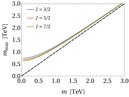
Figure 2: The maximal mass $m_{\mathrm{max}}$ of a scalar multiplet $\chi$ versus its lowest mass $m$, for three different values of the isospin $J$ of $\chi$.

One sees that heavy scalar multiplets tend to be almost degenerate; for $m\gtrsim 2$ TeV, $m_{\mathrm{max}}-m\sim 100$ GeV. Notice that $m_{\mathrm{max}}-m$ is maximal for $J=3/2$, i.e. when $\chi$ is a quadruplet; if $\chi$ is a larger multiplet, then it has more components but, as $\left|\lambda_{4}\right|_{\mathrm{maximal}}$ is smaller, those components are packed into an ever smaller mass range.

The maximum allowed value of $\lambda_{3}$ is always attained when $\lambda_{2}$ and all the $\lambda_{i}$ vanish, and exactly coincides with Eq. (37b), as is illustrated in the right panel of Fig. 1.

The minimum allowed value of $\lambda_{3}$ is always attained when both $\lambda_{4}$ and all the $\lambda_{i}$ are zero, but $\lambda_{2}$ is nonzero. Indeed, the minimum value of $\lambda_{3}$ is determined by the BFB condition (68b)—with $\lambda_{4}$ taken to zero—together with the UNI condition

$$\left|3\lambda_{1}+2\left(1+J\right)\lambda_{2}\right|+\sqrt{\left[3\lambda_{1}-2\left(1+J\right)\lambda_{2}\right]^{2}+8\left(1+2J\right)\lambda_{3}^{2}}\leq 2M,$$ (83)

which holds when all the $\lambda_{i}$ are taken to zero. Thus, when conditions (68b) and (83) are transformed into equations, they produce the solution

$$\lambda_{2} = \frac{1}{2}\,\frac{M\left(M-3\lambda_{1}\right)}{\left(1+J\right)M-\left(2+J\right)\lambda_{1}},$$ (84a)

$$\lambda_{3} = -\sqrt{\frac{\lambda_{1}}{2}\ \frac{M\left(M-3\lambda_{1}\right)}{\left(1+J\right)M-\left(2+J\right)\lambda_{1}}}.$$ (84b)

Equation (84b) gives the minimum value of $\lambda_{3}$ in the fourth row of Table 1.

4 Oblique parameters

In our NP model it is possible—depending on the values of $J$ and $Y$—that the new scalars do not couple to the light fermions at all. If that is so and if, moreover, the new scalars are very heavy, so that they cannot be produced at the LHC—for instance through the Drell–Yan process—then they will make themselves felt only indirectly through their oblique corrections, i.e. through their contributions to the self-energies of the gauge bosons. Following Maksymyk et al. [12], we parameterize those corrections through six oblique parameters (OPs) $S$, $T$, $U$, $V$, $W$, and $X$. We use as input of the renormalization process the quantities $\alpha$ (the fine-structure constant), $G_{F}$ (the Fermi coupling constant), and $m_{Z}$ (the $Z^{0}$ boson mass). Following Ref. [14], we use $\alpha\left(m^{2}_{Z}\right)=1\!\left/127.951\right.$, $G_{F}=1.1663788\times 10^{-5}$ GeV^-2, and $m_{Z}=91.1876$ GeV. We then define the weak mixing angle $\theta_{W}$ through

$$c_{W}^{2}s_{W}^{2}=\frac{\pi\alpha}{\sqrt{2}G_{F}m_{Z}^{2}},$$ (85)

where $c_{W}\equiv\cos{\theta_{W}}$ and $s_{W}\equiv\sin{\theta_{W}}$. This results in $s_{W}^{2}=0.23356$. We then use $S,\ldots,X$ to parameterize, for each electroweak observable $O$, the ratio between the prediction of the NP model and the prediction of the SM, by using expressions of the general form

$$\frac{O_{\mathrm{NP}}}{O_{\mathrm{SM}}}=1+c_{S}^{O}S+c_{T}^{O}T+c_{U}^{O}U+c_{V}^{O}V+c_{W}^{O}W+c_{X}^{O}X,$$ (86)

where the coefficients $c_{S}^{O},\ldots,c_{X}^{O}$—given for instance in Ref. [13]—are known functions of the input quantities.

4.1 Formulas for the OPs

According to Ref. [11], when in the NP Model there is only one $SU(2)$ multiplet of new scalars with weak isospin $J$ and weak hypercharge $Y$, the parameter $T$ produced by those scalars is given by

$$T=\frac{G_{F}}{8\sqrt{2}\pi^{2}\alpha}\ \sum_{I=1-J}^{J}\left(J^{2}+J-I^{2}+I\right)\theta_{+}\left(m_{I}^{2},m_{I-1}^{2}\right),$$ (87)

where $m_{I}$ denotes the mass of the scalar with third component of isospin $I$. The function $\theta_{+}\left(x,y\right)$ is defined as

$$\theta_{+}\left(x,y\right)\equiv\left\{\begin{array}[]{l}\displaystyle{x+y-\frac{2xy}{x-y}\,\ln{\frac{x}{y}}}\Leftarrow x\neq y,\\[5.69054pt] 0\Leftarrow x=y.\end{array}\right.$$ (88)

The parameters $V$, $W$, and $X$ are given by

$$V = \frac{G_{F}m_{Z}^{2}}{\sqrt{2}\pi^{2}\alpha}\ \sum_{I=-J}^{J}\left(Ic_{W}^{2}-Ys_{W}^{2}\right)^{2}\,\rho\left(\frac{m_{I}^{2}}{m_{Z}^{2}},\frac{m_{I}^{2}}{m_{Z}^{2}}\right),$$ (89a)

$$W = \frac{1}{4\pi s_{W}^{2}}\,\sum_{I=1-J}^{J}\left(J^{2}+J-I^{2}+I\right)\rho\left(\frac{m_{I}^{2}}{m_{W}^{2}},\frac{m_{I-1}^{2}}{m_{W}^{2}}\right),$$ (89b)

$$X = -\frac{1}{2\pi}\,\sum_{I=-J}^{J}\left(I+Y\right)\left(Ic_{W}^{2}-Ys_{W}^{2}\right)\,\zeta\left(\frac{m_{I}^{2}}{m_{Z}^{2}},\frac{m_{I}^{2}}{m_{Z}^{2}}\right),$$ (89c)

respectively. In Eqs. (89),

$$\zeta\left(x,y\right) = \frac{11}{36}-\frac{5\left(x+y\right)}{12}+\frac{xy}{3\left(x-y\right)^{2}}+\frac{\left(x-y\right)^{2}}{6}$$ (90a)

$$+\left[\frac{x^{2}-y^{2}}{4}+\frac{\left(y-x\right)^{3}}{12}+\frac{x^{2}+y^{2}}{4\left(y-x\right)}+\frac{x+y}{12\left(x-y\right)}+\frac{xy\left(x+y\right)}{6\left(y-x\right)^{3}}\right]\ln{\frac{x}{y}}$$

$$+\frac{\Delta\left(x,y\right)}{12}\ f\left(x,y\right),$$

$$\rho\left(x,y\right) = \frac{1}{6}-\frac{3\left(x+y\right)}{4}+\frac{\left(x-y\right)^{2}}{2}+\left[\frac{\left(y-x\right)^{3}}{4}+\frac{x^{2}+y^{2}}{4\left(y-x\right)}+\frac{x^{2}-y^{2}}{2}\right]\ln{\frac{x}{y}}$$ (90b)

$$+\frac{\left(x-y\right)^{2}-x-y}{4}\ f\left(x,y\right),$$

for $x\neq y$, while

$$\zeta\left(x,x\right) = \frac{4}{9}-\frac{4x}{3}+\frac{\Delta\left(x,x\right)}{12}\ f\left(x,x\right),$$ (91a)

$$\rho\left(x,x\right) = \frac{1}{6}-2x-\frac{x}{2}\ f\left(x,x\right).$$ (91b)

In Eqs. (90) and (91),

$$f\left(x,y\right)=\left\{\begin{array}[]{l}\displaystyle{\sqrt{\Delta\left(x,y\right)}\ \ln{\frac{x+y-1+\sqrt{\Delta\left(x,y\right)}}{x+y-1-\sqrt{\Delta\left(x,y\right)}}}\,\Leftarrow\Delta\left(x,y\right)\geq 0,}\\[11.38109pt] \displaystyle{-2\sqrt{-\Delta\left(x,y\right)}\left[\arctan{\frac{x-y+1}{\sqrt{-\Delta\left(x,y\right)}}}+\left(x\leftrightarrow y\right)\right]\Leftarrow\Delta\left(x,y\right)<0,}\end{array}\right.$$ (92)

where

$$\Delta\left(x,y\right)=1-2\left(x+y\right)+\left(x-y\right)^{2}.$$ (93)

For $S$ and $U$ one has

$$S=S^{\prime}+S^{\prime\prime},\quad U=U^{\prime}+U^{\prime\prime}.$$ (94)

where

$$S^{\prime\prime} = -\frac{2}{\pi}\,\sum_{I=-J}^{J}\left(Ic_{W}^{2}-Ys_{W}^{2}\right)^{2}\,\zeta\left(\frac{m_{I}^{2}}{m_{Z}^{2}},\frac{m_{I}^{2}}{m_{Z}^{2}}\right),$$ (95a)

$$U^{\prime\prime} = -S^{\prime\prime}-\frac{1}{\pi}\,\sum_{I=1-J}^{J}\left(J^{2}+J-I^{2}+I\right)\zeta\left(\frac{m_{I}^{2}}{m_{W}^{2}},\frac{m_{I-1}^{2}}{m_{W}^{2}}\right),$$ (95b)

and

$$S^{\prime} = -\frac{Y}{3\pi}\,\sum_{I=-J}^{J}I\,\ln{\frac{m_{I}^{2}}{\mu^{2}}},$$ (96a)

$$U^{\prime} = \frac{1}{12\pi}\,\sum_{I=1-J}^{J}\left(J^{2}+J-I^{2}+I\right)g\left(\frac{m_{I}^{2}}{m_{I-1}^{2}}\right)+\frac{1}{6\pi}\,\sum_{I=-J}^{J}\left(J^{2}+J-3I^{2}\right)\ln{\frac{m_{I}^{2}}{\mu^{2}}}.\hskip 28.45274pt$$ (96b)

In Eq. (96b),

$$g\left(x\right)=\left\{\begin{array}[]{l}{\displaystyle\frac{x^{3}-3x^{2}-3x+1}{\left(x-1\right)^{3}}\,\ln{x}-\frac{5x^{2}-22x+5}{3\left(x-1\right)^{2}}}\ \Leftarrow\ x\neq 1,\\[5.69054pt] 0\ \Leftarrow\ x=1\end{array}\right.$$ (97)

is a function that obeys $g\left(x\right)=g\left(1/x\right)$.

We note that the expresions for the OPs are invariant under the transformation $I\to-I,\ Y\to-Y$. This allows one to choose the scalar with $I=-J$ to be the lightest one, provided one keeps $Y$ free, i.e. provided one considers both negative and positive values of $Y$; that is the procedure that we adopt.

4.2 Numerical results

In our numerical work we utilize the set of electroweak observables given in Table 2.

Observable	Measurement ($O_{\mathrm{meas}}$)	SM prediction ($O_{\mathrm{SM}}$)	$O_{\mathrm{meas}}/O_{\mathrm{SM}}$
$\sigma^{0}_{\textrm{had}}$ [nb]	$41.481\,\pm\,0.033$	$41.482\,\pm\,0.008$	$0.999976\,\pm\,0.0008186$
$R_{\ell}$	$20.767\,\pm\,0.025$	$20.736\,\pm\,0.010$	$1.00149\,\pm\,0.001299$
$R_{b}$	$0.21629\,\pm\,0.00066$	$0.21582\,\pm\,0.00002$	$1.00218\,\pm\,0.003060$
$R_{c}$	$0.1721\,\pm\,0.0030$	$0.17221\,\pm\,0.00003$	$0.999361\,\pm\,0.01742$
$A_{FB}^{(0,\ell)}$	$0.0171\,\pm\,0.001$	$0.01617\,\pm\,0.00007$	$1.05751\,\pm\,0.06201$
$A_{FB}^{(0,b)}$	$0.0996\,\pm\,0.0016$	$0.1029\,\pm\,0.0002$	$0.967930\,\pm\,0.01566$
$A_{FB}^{(0,c)}$	$0.0707\,\pm\,0.0035$	$0.0735\,\pm\,0.0002$	$0.961905\,\pm\,0.04769$
$A_{\ell}$	$0.1513\,\pm\,0.0021$	$0.1468\,\pm\,0.0003$	$1.03065\,\pm\,0.01446$
$A_{b}$	$0.923\,\pm\,0.020$	$0.9347$	$0.987483\,\pm\,0.02140$
$A_{c}$	$0.670\,\pm\,0.027$	$0.6677\,\pm\,0.0001$	$1.00344\,\pm\,0.04044$
$\bar{s}_{\ell}^{2}\leavevmode\nobreak\ (\textrm{LEP-1})$	$0.2324\,\pm\,0.0012$	$0.23155\,\pm\,0.00004$	$1.00367\,\pm\,0.005185$
$\bar{s}_{\ell}^{2}\leavevmode\nobreak\ (\textrm{Tevt.})$	$0.23148\,\pm\,0.00033$	$0.23155\,\pm\,0.00004$	$0.999698\,\pm\,0.001436$
$\bar{s}_{\ell}^{2}\leavevmode\nobreak\ (\textrm{LHC})$	$0.23129\,\pm\,0.00033$	$0.23155\,\pm\,0.00004$	$0.998877\,\pm\,0.001436$
$m_{W}$ [GeV]	$80.377\,\pm\,0.012$	$80.360\,\pm\,0.006$	$1.00021\,\pm\,0.0001670$
$\Gamma_{W}$ [GeV]	$2.046\,\pm\,0.049$	$2.089\,\pm\,0.001$	$0.979416\,\pm\,0.02346$
$\Gamma_{Z}$ [GeV]	$2.4955\,\pm\,0.0023$	$2.4941\,\pm\,0.0009$	$1.00056\,\pm\,0.0009903$
$g_{V}^{\nu e}$	$-0.040\,\pm\,0.015$	$-0.0397\,\pm\,0.0001$	$1.00756\,\pm\,0.37784$
$g_{A}^{\nu e}$	$-0.507\,\pm\,0.014$	$-0.5064$	$1.00118\,\pm\,0.02765$
$Q_{W}(\mathrm{Cs})$	$-72.82\,\pm\,0.42$	$-73.24\,\pm\,0.01$	$0.994265\,\pm\,0.005736$
$Q_{W}(\mathrm{Tl})$	$-116.4\,\pm\,3.6$	$-116.90\,\pm\,0.02$	$0.995723\,\pm\,0.03080$

Table 2: First column: the electroweak observables used in our work. Second column: their experimental values, taken from Ref. [14]. Third column: the SM predictions for them. Fourth colum: the ratio between the experimental value and the SM prediction.

For each set of OPs and for each observable $O$, we have computed $\left.O_{\mathrm{NP}}\right/O_{\mathrm{SM}}$ by using Eq. (86). We have then computed the residuals, defined as $\left.O_{\mathrm{NP}}\right/O_{\mathrm{SM}}$ minus the values in the last column of Table 2. The $\chi^{2}$ function for each set of OPs was defined as $\chi^{2}=RC^{-1}R^{T}$, where $R$ is the row-vector of the residuals and $C$ is the covariance matrix; the latter is evaluated according to the correlations among the observables [14, 15, 16].

For each set of OPs, the pull is evaluated as $\left.r\right/\delta^{\pm}$, where $r$ is the residual defined above and $\delta^{\pm}$ is the error given in the fourth column of Table 2.

Firstly, setting $V=W=X=0$ and freely adjusting $S$, $T$, and $U$ we have accomplished our best fit of the electroweak observables in Table 2. We have obtained $\chi^{2}=14.201$ for $S=-1.2\times 10^{-2}$, $T=2.8\times 10^{-2}$, and $U=2.0\times 10^{-3}$.

In our NP model, for each value of the isospin $J$ of the multiplet, there are just three free parameters:

$\left|\lambda_{4}\right|$, which determines the mass-squared difference $\Delta m^{2}=\left.\left|\lambda_{4}\right|v^{2}\right/2$ between any two successive components of the multiplet.

The mass $m$ of the lightest component of the multiplet; without loss of generality we take that component to be the one with the smallest third projection of isospin. Thus, $m_{I}^{2}=m^{2}+\left(I+J\right)\Delta m^{2}$ for $I=-J,\ldots,$.

The hypercharge $Y$ of the multiplet.

For instance, by choosing $J=2$, $m=2$ TeV, $\lambda_{4}=2$, and $Y=3$ we have obtained $\chi^{2}=14.236$, which is not very far from our best fit. We thus see that our model is able to fit the electroweak observables just as perfectly as a free fit.

For each value of $J$ up to $7/2$—the upper bound on $J$ found in Ref. [4]—we let $Y$ vary from $-Y_{\mathrm{max}}$ to $Y_{\mathrm{max}}$, where $Y_{\mathrm{max}}$ is the $J$-dependent upper bound on $\left|Y\right|$ determined in Refs. [4, 5]. We let $m$ vary from 50 GeV to 3 TeV, and we let $\left|\lambda_{4}\right|$ vary from zero to its maximum allowed value given in Table 1. We keep only the points that either

1. have $\chi^{2}$ smaller than 30 and all the pulls smaller (in modulus) than three,

2. or have $\chi^{2}$ smaller than 17 and all the pulls smaller than one, except, possibly, the pulls of $A_{FB}^{\left(0,b\right)}$, $A_{\ell}$, $R_{\ell}$, and $Q_{W}\!\left(\mathrm{Cs}\right)$.

In this way we obtain two sets of points, that we use to construct Figures 3 and 4 below. Most pulls of the observables are always very small; only a few observables have large pulls. As a consequence, in practice, points with $\chi^{2}<30$ mostly have all the pulls between $-3$ and $+3$, and points with $\chi^{2}<17$ almost always have all the pulls between $-1$ and $+1$, except for the observables $A_{FB}^{\left(0,b\right)}$ $A_{\ell}$, $R_{\ell}$, and $Q_{W}\!\left(\mathrm{Cs}\right)$.

One sees in Fig. 3 that, unless $m$ is very large and, therefore, the OPs are very small, the restrictions on $\left|\lambda_{4}\right|$ from the OPs are usually stronger that the UNI and BFB conditions that we have derived in this paper. Indeed, for $\chi^{2}\leq 30$ and $m\lesssim 2$ TeV the restrictions from the OPs are stronger, and the same happens for $\chi^{2}\leq 17$ and $m\lesssim 3$ TeV.

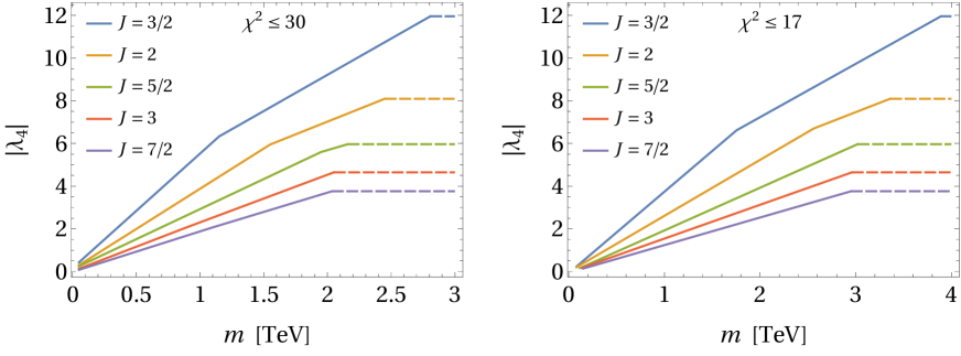
Figure 3: The maximum allowed value of $\left|\lambda_{4}\right|$ versus the lightest mass $m$, for various values of $J$ and for fits with $\chi^{2}\leq 30$ (left panel) or $\chi^{2}\leq 17$ (right panel). The hypercharge $Y$ was left free. The horizontal dashed lines correspond to the bounds on $\left|\lambda_{4}\right|$ from the UNI and BFB conditions.

The relation between the upper bound on $\left|\lambda_{4}\right|$ and the hypercharge $Y$ is quite complex and very much depends on $m$ (because, if $m$ gets larger, then the OPs get smaller and therefore the OPs do not constrain $\left|\lambda_{4}\right|$). In Fig. 4, which was made for $m=3$ TeV, one observes that, as $Y$ increases, the upper bound on $\left|\lambda_{4}\right|$ slightly decreases.

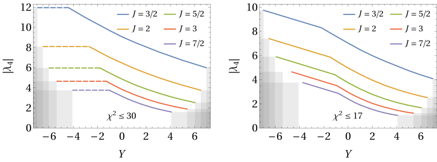
Figure 4: The upper bound on $\left|\lambda_{4}\right|$ versus the hypercharge $Y$, for various values of $J$, for $m=3$ TeV, and for fits with $\chi^{2}\leq 30$ (left panel) or $\chi^{2}\leq 17$ (right panel). The horizontal dashed lines indicate the upper bounds from the UNI and BFB conditions, and the curved lines indicate the upper bounds from the OPs. The gray bands indicate the $J$-dependent restrictions on $Y$ derived in Refs. [4, 5].

If one requires a smaller $\chi^{2}$ in the fit of the oblique parameters, then the constraint on $\left|\lambda_{4}\right|$ derived therefrom becomes stronger and eventually, as one sees in the right panel of Fig. 4, the UNI+BFB bound becomes completely ineffective.

5 Conclusions and outlook

In this paper we have studied the extension of the SM through a scalar multiplet $\chi$ with arbitrary isospin $J$ and hypercharge $Y$. For every value of $J$, we have included in the scalar potential (SP) just those terms that are present there for any value of $Y$. We have especially concentrated on the term (1), which fixes the squared-mass difference $\Delta m^{2}$ between the successive components of $\chi$, cf. Eq. (15). We have derived an upper bound on $\left|\lambda_{4}\right|$, hence on $\Delta m^{2}$, from both the unitarity (UNI) and bounded-from-below (BFB) conditions on the SP. We have found that, remarkably, that upper bound depends crucially, not just on the UNI conditions, but also on the BFB ones. For instance, the upper bound that we have found is quite more stringent than the one utilized in the recent Ref. [17], which used only UNI conditions.

Remarkably, we have been able to derive necessary and sufficient BFB conditions on this model, even when we allowed the presence in the SP of the most general terms four-linear in the components of $\chi$. It so happens that those terms, even if they are quite complicated to account for, end up relaxing only a little bit the upper bound on $\left|\lambda_{4}\right|$, cf. Fig. 1.

Phenomenologically, the model that we have studied is, by itself alone, of little value, because, since we have left $Y$ arbitrary, the multiplet $\chi$ does not have Yukawa couplings to any fermions. Moreover, its lightest component is, for arbitrary $Y$, electrically charged and, moreover, absolutely stable, which is of course incompatible with observation. Therefore, our study can only be understood as a step towards the understanding of more specific models, that will have precise values of $J$ and $Y$, and probably also extra terms in the scalar potential, viz. higher-dimensional terms.

Acknowledgements:

L.L. thanks Kristjan Kannike for a discussion on Ref. [6] and for having called his attention to Ref. [10]. The work of D.J. was supported by the Lithuanian Particle Physics Consortium. The work of L.L. was supported by the Portuguese Foundation for Science and Technology through projects UIDB/00777/2020, UIDP/00777/2020, CERN/FIS-PAR/0002/2021, and CERN/FIS-PAR/0019/2021.

Appendix A Explicit UNI conditions

For $J$ through $7/2$, the unitarity conditions that originate in the matrix $\mathcal{S}$ of Eq. (75) are, besides Eqs. (78), the following:

• For $J=1$,

  $$\left|\lambda_{2}+\frac{4}{3}\,\lambda_{5}\right|<M.$$ (A1)

• For $J=3/2$,

  $$\left|\lambda_{2}+\frac{3}{5}\,\lambda_{5}\right| < M,$$ (A2a)

  $$\left|\lambda_{2}+\frac{9}{5}\,\lambda_{5}\right| < M.$$ (A2b)

• For $J=2$,

  $$\left|\lambda_{2}+\frac{16}{7}\,\lambda_{5}-\frac{4}{5}\,\lambda_{6}\right| < M,$$ (A3a)

  $$\left|\lambda_{2}+\frac{8}{7}\,\lambda_{5}+\frac{4}{5}\,\lambda_{6}\right| < M,$$ (A3b)

  $$\left|\lambda_{2}-\frac{6}{7}\,\lambda_{5}+\frac{4}{5}\,\lambda_{6}\right| < M.$$ (A3c)

• For $J=5/2$,

  $$\left|\lambda_{2}+\frac{79}{45}\,\lambda_{5}-\frac{22}{35}\,\lambda_{6}\right| < M,$$ (A4a)

  $$\left|\lambda_{2}+\frac{19}{9}\,\lambda_{5}-\frac{2}{7}\,\lambda_{6}\right| < M,$$ (A4b)

  $$\left|\lambda_{2}+\frac{5}{9}\,\lambda_{5}+\frac{10}{7}\,\lambda_{6}\right| < M,$$ (A4c)

  $$\left|\lambda_{2}-\frac{29}{15}\,\lambda_{5}+\frac{46}{35}\,\lambda_{6}\right| < M.$$ (A4d)

• For $J=3$,

  $$\left|\lambda_{2}+\frac{102}{77}\,\lambda_{5}+\frac{25}{21}\,\lambda_{6}-\frac{4}{7}\,\lambda_{7}\right| < M,$$ (A5a)

  $$\left|\lambda_{2}+\frac{18}{77}\,\lambda_{5}+\frac{25}{21}\,\lambda_{6}+\frac{4}{7}\,\lambda_{7}\right| < M,$$ (A5b)

  $$\left|\lambda_{2}+\frac{6}{7}\,\lambda_{5}+\frac{10}{21}\,\lambda_{6}-\frac{4}{7}\,\lambda_{7}\right| < M,$$ (A5c)

  $$\left|\lambda_{2}-\frac{18}{7}\,\lambda_{5}+\frac{19}{21}\,\lambda_{6}+\frac{4}{7}\,\lambda_{7}\right| < M,$$ (A5d)

  $$\left|\lambda_{2}+\frac{194}{77}\,\lambda_{5}-\frac{10}{7}\,\lambda_{6}+\frac{4}{7}\,\lambda_{7}\right| < M.$$ (A5e)

• For $J=7/2$,

  $$\left|\lambda_{2}-\frac{1}{14}\,\lambda_{5}+\frac{31}{22}\,\lambda_{6}-\frac{13}{14}\,\lambda_{7}\right| < M,$$ (A6a)

  $$\left|\lambda_{2}+\frac{53}{78}\,\lambda_{5}+\frac{119}{66}\,\lambda_{6}-\frac{1}{2}\,\lambda_{7}\right| < M,$$ (A6b)

  $$\left|\lambda_{2}+\frac{363}{182}\,\lambda_{5}-\frac{1}{22}\,\lambda_{6}-\frac{1}{14}\,\lambda_{7}\right| < M,$$ (A6c)

  $$\left|\lambda_{2}+\frac{7}{78}\,\lambda_{5}+\frac{49}{66}\,\lambda_{6}+\frac{7}{6}\,\lambda_{7}\right| < M,$$ (A6d)

  $$\left|\lambda_{2}-\frac{121}{42}\,\lambda_{5}+\frac{1}{6}\,\lambda_{6}+\frac{17}{14}\,\lambda_{7}\right| < M,$$ (A6e)

  $$\left|\lambda_{2}+\frac{103}{66}\,\lambda_{5}-\frac{101}{66}\,\lambda_{6}+\frac{23}{42}\,\lambda_{7}\right| < M.$$ (A6f)

References

- [1] L. Lavoura and L.-F. Li (1994). Making the small oblique parameters large. Physical Review D 49, 1409 [e-Print: hep-ph/9309262 [hep-ph]].
- [2] M. Cirelli, N. Fornengo, and A. Strumia (2006). Minimal dark matter. Nuclear Physics B 753, 178 [e-Print: hep-ph/0512090 [hep-ph]].
- [3] J. Wu, D. Huang, and C.-Q. Geng (2023). -boson mass anomaly from a general scalar multiplet. Chinese Physics C 47, 063103 [e-Print: 2212.14553 [hep-ph]].
- [4] K. Hally, H. E. Logan, and T. Pilkington (2012). Constraints on large scalar multiplets from perturbative unitarity. Physical Review D 85, 095017 [e-Print: 1202.5073 [hep-ph]].
- [5] A. Milagre and L. Lavoura (2024). Unitarity constraints on large multiplets of arbitrary gauge groups. E-Print: 2403.12914 [hep-ph].
- [6] K. Kannike (2024). Constraining the Higgs trilinear coupling from an quadruplet with bounded-from-below conditions. Journal of High Energy Physics 2024, 176 [e-Print: 2311.17995 [hep-ph]].
- [7] A. Giarnetti, J. Herrero-García, S. Marciano, D. Meloni, and D. Vatsyayan (2024). Neutrino masses from new Weinberg-like operators: Phenomenology of TeV scalar multiplets. E-Print: 2312.13356 [hep-ph].
- [8] A. Giarnetti, J. Herrero-García, S. Marciano, D. Meloni, and D. Vatsyayan (2024). Neutrino masses from new seesaw models: Low-scale variants and phenomenological implications. E-Print: 2312.14119 [hep-ph].
- [9] K. Kannike (2012). Vacuum stability conditions from copositivity criteria. The European Physical Journal C 72, 2093 [e-Print: 1205.3781 [hep-ph]].
- [10] C. Bonilla, R. M. Fonseca, and J. W. F. Valle (2015). Consistency of the triplet seesaw model revisited. Physical Review D 92, 075028 [e-Print: 1508.02323 [hep-ph]].
- [11] F. Albergaria and L. Lavoura (2023). Oblique corrections from leptoquarks. Journal of High Energy Physics 2023, 080 [e-Print: 2301.03024 [hep-ph]].
- [12] I. Maksymyk, C. P. Burgess, and D. London (1994). Beyond , , and . Physical Review D 50, 529 [e-Print: hep-ph/9306267 [hep-ph]].
- [13] S. Draukšas, V. Dūdėnas, and L. Lavoura (2024). Oblique parameters when at tree level. To be published in Pramana [E-Print: 2305.14050 [hep-ph]].
- [14] Particle Data Group, R. L. Workman et al. (2022). Review of Particle Physics. Progress in Theoretical and Experimental Physics 2022, 083C01.
- [15] S. Schael et al. [ALEPH, DELPHI, L3, OPAL, SLD, LEP Electroweak Working Group, SLD Electroweak Group, and SLD Heavy Flavour Group] (2006). Precision electroweak measurements on the resonance. Physics Reports 427, 257 [e-Print: hep-ex/0509008 [hep-ex]].
- [16] R. Tenchini (2016). Asymmetries at the Z pole: The Quark and Lepton Quantum Numbers. Advanced Series on Directions in High Energy Physics 26, 161.
- [17] J. Wu, D. Huang, and C.-Q. Geng (2024). -boson Mass Anomaly from High-Dimensional Scalar Multiplets. E-Print: 2307.12105 [hep-ph].