Non-Markovian dynamics with a giant atom coupled to a semi-infinite photonic waveguide

Abstract

We study the non-Markovian dynamics of a two-level giant atom interacting with a one-dimensional semi-infinite waveguide through multiple coupling points, where a perfect mirror is located at the endpoint of the waveguide. The system enters a non-Markovian process when the travel time of the photon between adjacent coupling points is sufficiently large compared to the inverse of the bare relaxation rate of the giant atom. The photon released by the spontaneous emission of the atom transfers between multiple coupling points through the waveguide or is reabsorbed by the atom with the photon emitted via the atom having completed the round trip after reflection of the mirror, which leads to the photon being trapped and forming bound states. We find that three different types of bound states can be formed in the system, containing the static bound states with no inversion of population, the periodic equal amplitude oscillation with two bound states, and the periodic non-equal amplitude oscillation with three bound states. The physical origins of three bound states formation are revealed. Moreover, we consider the influences of the dissipation of unwanted modes and dephasing on the bound states. Finally, we extend the system to a more general case involving many giant atoms coupled into a one-dimensional semi-infinite waveguide. The obtained set of delay differential equations for the giant atoms might open a way to better understand the non-Markovian dynamics of many giant atoms coupled to a semi-infinite waveguide.

I Introduction

The core topic of quantum optics Kockum192019 is the understanding and application of the interaction between light and matter. The study of the interaction between light and matter can be well carried out on platforms such as cavity quantum electrodynamics (QED) systems Kimble1271998 ; Raimond5652001 ; Walther13252006 , circuit-QED systems Blais0250052021 ; Blais0623202004 ; Wallraff1622004 , and waveguide QED systems Roy0210012017 ; Roy12017 ; Sheremet210306824 , the limited bandwidth of the waveguide QED systems can be relaxed Roy0210012017 because the waveguides usually support a continuous mode. These studies are usually based on point-like atoms, where the wavelength of light is usually much larger than the size of point-like atoms Wallraff1622004 ; Roy12017 ; Goy19031983 ; Leibfried2812003 ; Miller5512005 ; Haroche10832013 . Therefore, we usually use the dipole approximation Walls2008 to simplify the interaction between photons and atoms when dealing with these systems. With the deepening of quantum optics research and the great technological progress of superconducting circuits Manenti9752017 ; Roy12017 ; You5892011 ; Kockum2019 ; Krantz0213182019 , artificial giant atoms Roy0210012017 ; Roy12017 ; Gustafsson2072014 ; Kockum2021 ; Andersson11232019 ; Kannan7752020 that can interact with surface acoustic waves or microwaves through multiple coupling points have been designed in experiment. Since giant atoms can be designed to couple with waveguides at multiple points with large separation distances, the dipole approximation is no longer valid Gustafsson2072014 .

In systems containing giant atoms, many interesting and previously undiscovered phenomena resulting from quantum interference effects between multiple coupling points have been predicted, such as the frequency-dependent relaxation rate and the Lamb shift of giant atoms Kannan7752020 ; Kockum0138372014 ; Vadiraj200314167 , decoherence-free interaction between multiple giant atoms Kannan7752020 ; Kockum1404042018 ; Carollo0431842020 ; Du0237052023 ; Cilluffo0430702020 ; Soro023712 ; Soro0137102023 , non-exponential relaxation Andersson11232019 ; Guo053821017 ; Longhi30172020 ; Guo0337062020 ; Du0231982022 , generation of bound states Guo0430142020 ; Zhao0538552020 ; Wang0436022021 ; Lim0237162023 ; Xiao802022 ; Cheng0335222022 ; Yin0637032022 ; Vega0535222021 , and electromagnetically induced transparency Ask201115077 ; Zhao425062022 ; Zhu0437102022 , etc. Du2236022022 ; Zhang220503674 ; Noachtar0137022022 ; Du123012023 ; Wang0437032022 ; Brianso0637172022 ; Santos0536012023 ; Yang1151042021 ; Qiu2242122023 ; Wang0350072022 ; Burillo0137092020 ; Wang75802022 ; Liu742023 ; Du2236022022 ; Zhang230316480 ; Li35982023 ; Chen230414713 ; Wang230410710 ; Du0450102023 ; Kuo230707949 ; Jia230402072 ; Yin230314746 ; Liu1068542023 . The giant atom scheme provides an effective way to control photons Wang401162021 ; Zhang10542992022 ; Zhang1705682023 ; Du0237122021 ; Du30382021 ; Gu230613836 ; Cheng3382023 ; Cai0337102021 ; Feng0637122021 ; Zou8968272022 ; Yin013715 , especially the nonreciprocal propagation of photons Yu0137202021 ; Zhou0637032023 ; Du0537012021 ; Wang221101819 ; Du0432262021 ; Chen2152022 ; Liu234282022 ; Sun0351032023 . Moreover, the giant atom scheme can also achieve higher dimensional cold atomic structures in optical lattices Tudela2036032019 . In the past, many studies of non-Markovian systems were based on point-like atoms in the traditional framework of quantum optics, where the presence of mirrors or multiple point-like atoms is often required Eschner4952001 ; Tufarelli0121132014 ; Guimond0440122017 ; Calajo0736012019 ; Milonni10961974 ; Zheng1136012013 ; Ballestero0730152013 ; Laakso1836012014 ; Ballestero0423282014 ; Fang0538452015 ; Guimond0238082016 ; Ramos0621042016 ; Tufarelli0138202013 ; Dinc2132019 . However, the non-Markovianity of a single giant atom can be achieved by tuning the time delay between adjacent coupling points Guo053821017 ; Ask0138402019 in quantum systems containing giant atoms.

The majority of the work on giant atoms deals with two-level or three-level systems coupled to one-dimensional infinite waveguides. In fact, for one-dimensional waveguides, both ends are usually terminated by other media, and light can be partially reflected in waveguides due to the difference in refractive index. The single-ended and quasi-one-dimensional structures have been realized, for example, by thinning one end of the waveguide to make it almost transparent while the other end is connected to an opaque medium Claudon1742010 ; Bleuse1036012011 ; Reimer7372012 ; Bulgarini1211062012 . Such a system can be equivalent to an infinite waveguide with a mirror at one end Barkemeyer19000782020 ; Song592018 ; Bradford0638302013 ; Chang0243052020 ; Sinha0436032020 ; Fang043035043035 ; Zeng0303052023 ; Barkemeyer0237082022 ; Crowder0137142022 ; Xin0537062022 ; Barkemeyer0337042021 ; Kabuss102016 ; Ding230606373 ; Ding230716876 ; Wang19002252019 ; Wang111772019 . However, the non-Markovian dynamics for the two-level giant atom coupled to a semi-infinite waveguide still remains unexplored.

In this paper, we study the non-Markovian dynamics of a two-level giant atom coupled to a one-dimensional semi-infinite waveguide through multiple coupling points, where the finite end of the waveguide is realized by a perfect mirror. When the traveling time of a photon between the adjacent coupling points is sufficiently large compared to the inverse of the bare relaxation rate of the atom, the system enters a non-Markovian process. The photon is continuously transferred between multiple coupling points via the semi-infinite waveguide or is reabsorbed after the photon is reflected by the mirror. We find three different types of bound states, containing the static bound states, the periodic equal and non-equal amplitude oscillating bound states and discuss the physical origins of the bound states formation. We study the atomic dynamics and the corresponding field intensity distributions in the above three cases. Moreover, for a realistic waveguide QED setup in experiment, the light-matter interaction dominates over loss and dephasing, and we discuss the influence of this detrimental phenomenon on the formation of bound states. Finally, we extend the system to a non-Markovian quantum system with many giant atoms and one-dimensional semi-infinite waveguide coupling.

The paper is organized as follows. In Sec. II, we introduce our model, explain methods we used to tackle the non-Markovian dynamics, and give the dynamical equations of the waveguide and giant atom. In Sec. III, we derive the delay differential equation, field intensity function, and exact analytical expression for the probability amplitude of the giant atom. In Sec. IV, we discuss the conditions for the formation of bound states and obtain three different types of bound states. Sec. V gives the dynamical expressions of three different types of bound states and explores the influences of the different parameters on field intensity distribution. Moreover, the bound states under the different number of coupling points are also considered. In Sec. VI, we study the influences of the dissipation of unwanted modes and dephasing on the non-Markovian dynamics of the giant atom. In Sec. VII, we generalize the system to the case containing many two-level giant atoms coupling to a one-dimensional semi-infinite waveguide and derive a set of delay differential equations of the probability amplitude with different giant atoms. In Sec. VIII, all of the above work is summarized.

Figure 1: Schematic diagram of the scheme. A two-level giant atom is coupled to a one-dimensional semi-infinite waveguide via $N$ coupling points with coupling coefficient $g_{km}$, where the waveguide is terminated by a perfect mirror with reflectivity $R=1$ at $x=0$. The distance between the adjacent coupling points is the same as that between the mirror and the first coupling point, both of which are ${{x_{0}}}$. $\omega_{0}$ denotes the transition frequency between the ground state $|g\rangle$ and the excited state $|e\rangle$ of the giant atom.

II Model Hamiltonian

We consider a two-level giant atom coupled to a one-dimensional semi-infinite waveguide through $N$ coupling points, which can be realized by photonic crystal waveguide Wang4201832018 ; Wang8168702018 ; Lodahl4306542004 and microwave transmission line Roy12017 ; Peropadre0638342011 ; Mok0538612020 ; Boch1705012014 ; Eichler0321062012 . As shown in Fig. 1, one end of the waveguide $(x=0)$ is terminated by a perfect mirror with the reflectivity $R=1$, allowing the photon emitted through the atom to transfer between the mirror and each coupling point via the waveguide. The dispersion relationship of the photon with the wave vector $k$ in the waveguide is approximately linear around the transition frequency ${\omega_{0}}$ as ${\Omega_{k}}\simeq{\omega_{0}}+v(k-{k_{0}})$ Roy0210012017 ; Shen3020012005 ; Shen0238372009 ; Shen0238382009 ; Shen2130012005 , where $v$ is the photon group velocity, and ${\Omega_{{k_{0}}}}={\omega_{0}}$. Any $k>0$ in the infinite waveguide corresponds to two orthogonal static modes with spatial profiles of $\propto\cos(kx)$ and $\propto\sin(kx)$, respectively. However, for a semi-infinite waveguide, we only need to consider the sinelike modes because there is a perfect mirror at one end of the waveguide. Therefore, the giant atom interacts with the waveguide at the $m\mathrm{th}$ coupling point with coupling strength ${g_{km}}\propto\sin(km{x_{0}})(m=1,~{}2,~{}...,~{}N)$. Under the rotating-wave approximation, the Hamiltonian of the system reads $(\hbar=1)$

$$\hat{H} ={\hat{H}_{a}}+{\hat{H}_{w}}+{\hat{H}_{aw}},$$ (1)

$${\hat{H}_{a}} ={\omega_{0}}\left|e\right\rangle\left\langle e\right|,$$

$${\hat{H}_{w}} =\int_{0}^{{k_{c}}}{dk}{\Omega_{k}}\hat{a}_{k}^{\dagger}{{\hat{a}}_{k}},$$

$${\hat{H}_{aw}} =\sum\limits_{m=1}^{N}{\int_{0}^{{k_{c}}}{dk}({g_{km}\hat{a}_{k}^{\dagger}{\sigma_{-}}}+{g^{*}_{km}}\hat{a}_{k}{\sigma_{+}})},$$

where ${\hat{H}_{a}}$ and ${\hat{H}_{w}}$ denote the free Hamiltonian of the atom and waveguide, respectively. ${\hat{H}_{aw}}$ describes the interaction between the atom and the semi-infinite waveguide. ${{k_{c}}}$ stands for a cutoff wave vector depending on a specific waveguide. We define the raising operator (lowering operator) of the atom as ${\sigma_{+}}=\left|e\right\rangle\left\langle g\right|({\sigma_{-}}=\left|g\right\rangle\left\langle e\right|)$, where $\left|e\right\rangle$ and $\left|g\right\rangle$ denote excited and ground states, respectively. $\hat{a}_{k}^{\dagger}({{\hat{a}}_{k}})$ is the photon generation (annihilation) operator, which satisfies the $[{{{\hat{a}}_{k}},\hat{a}_{k^{\prime}}^{\dagger}}]=\delta(k-k^{\prime})$. Moreover, we set the distance between adjacent coupling points equal to ${x_{0}}$ (the distance between the endpoint of a semi-infinite waveguide and the first coupling point is also ${x_{0}}$). Therefore, the time for the photon to travel between any two adjacent coupling points (including between the endpoint of a semi-infinite waveguide and the first coupling point) is a constant ${\tau_{0}}={x_{0}}/v$. In this paper, we explore the non-Markovian dynamics caused by the time delay ${\tau_{0}}$ induced through adjacent coupling points and the semi-infinite waveguide for the giant atom.

We choose $\left|{e,0}\right\rangle$ as the initial state, where the atom is in the excited state $\left|e\right\rangle$, while the field in the waveguide remains in the vacuum state $\left|0\right\rangle$. As we work under the rotating-wave approximation, the processes we are interested in involve a narrow range of wave vectors around $k={k_{0}}$, and the boundary of the integral can be changed to $\int_{0}^{{k_{c}}}{dk}\to\int_{-\infty}^{+\infty}{dk}$ Roy0210012017 ; Shen3020012005 ; Zhang0323352020 ; Liao0630042016 . Since the total number of atomic and field excitations in the system is conserved, the state of the total system in the single excitation subspace can be written as

$$\left|{\psi(t)}\right\rangle=\varepsilon(t)\left|{e,0}\right\rangle+\int{dk\varphi(k,t)}\hat{a}_{k}^{\dagger}\left|{g,0}\right\rangle,$$ (2)

where $\varepsilon(t)$ denotes the probability amplitude of the giant atom in the excited state $\left|e\right\rangle$, while the second term on the right side of Eq. (2) describes the state of a single boson propagating in the waveguide with the probability amplitude $\varphi(k,t)$. Substituting Eqs. (1) and (2) into Schrödinger equation $i\partial_{t}\left|\psi\right\rangle=\hat{H}\left|\psi\right\rangle$, we get the set of differential equations of the probability amplitudes

$$\dot{\varepsilon}(t) = -i{\omega_{0}}\varepsilon(t)-i\sum\limits_{m=1}^{N}{\int{dk{g_{km}^{*}}\varphi(k,t)}},$$ (3)

$$\dot{\varphi}(k,t) = -i{\Omega_{k}}\varphi(k,t)-i\sum\limits_{m=1}^{N}{g_{km}\varepsilon(t)},$$ (4)

which determine the dynamical evolutions for the giant atom and the semi-infinite waveguide.

III Equation of motion and the solution

In this section, we derive the analytical expressions for the probability amplitude of the two-level giant atom by solving a set of delay differential equations. We set the coupling strength as ${g_{km}}=\sqrt{\Gamma v/\pi}\sin(km{x_{0}})$ Tufarelli0121132014 , where $\Gamma$ denotes the spontaneous emission rate of the atom without a mirror. By substituting the coupling strength ${g_{km}}$ and initial condition $\varphi(k,0)=0$ into Eqs. (3) and (4), we can obtain the atomic excitation probability amplitude

$$\dot{\varepsilon}(t)= -i{\omega_{0}}\varepsilon(t)$$ (5)

$$-\frac{\Gamma}{2}\sum\limits_{m,n=1}^{N}{\varepsilon(t-\left|{m-n}\right|{\tau_{0}})\Theta(t-\left|{m-n}\right|{\tau_{0}})}$$

$$+\frac{\Gamma}{2}\sum\limits_{m,n=1}^{N}{\varepsilon\left[{t-(m+n){\tau_{0}}}\right]\Theta\left[{t-(m+n){\tau_{0}}}\right]},$$

where $\Theta(x)$ denotes the Heaviside step function, which describes the delayed feedback from the coupling points and the reflection of the semi-infinite waveguide. The first term on the right side of Eq. (5) describes atomic coherent dynamics. The second term on the right side of Eq. (5) indicates that the photon transfers from the $m$th coupling point to the $n$th coupling point without being reflected by the mirror, including the Markovian approximation that the photon released from the $m$th coupling point is reabsorbed at the same point without the reflection of the mirror. The last term on the right side of Eq. (5) denotes the feedback term that the photon released from the $m$th coupling point is absorbed by the $n$th coupling point after being reflected through the mirror. The atomic reabsorption of the emitted photon denoted in the second and third terms of Eq. (5) occurs at the evolution time $t\geqslant\left|{m-n}\right|{\tau_{0}}$ and $t\geqslant(m+n){\tau_{0}}$, respectively. Moreover, we find the probability amplitude with the giant atom in Eq. (5) can be reduced to that with the point-like atom in Ref. Tufarelli0121132014 when $m=n=1$.

In addition to the dynamics of the atom, the dynamical characteristics of the output field are also crucial. The annihilation operator of the photon in real space is $\hat{C}(x)=\sqrt{2/\pi}\int{dk}{{\hat{a}}_{k}}\sin(kx)$, and $\hat{C}(x)\left|{\psi(t)}\right\rangle=\phi(x,t)\left|{g,0}\right\rangle$ can be obtained by substituting $\hat{C}(x)$ into Eq. (2). Therefore, the probability amplitude $\phi(x,t)=\sqrt{2/\pi}\int{dk}\varphi(k,t)\sin(kx)$ of the real space field is

$$\phi(x,t)= -i\sqrt{\frac{\Gamma}{{2v}}}\sum\limits_{m=1}^{N}{\varepsilon({t-|{\tau-m{\tau_{0}}}|})\Theta({t-|{\tau-m{\tau_{0}}}|})}$$ (6)

$$+i\sqrt{\frac{\Gamma}{{2v}}}\sum\limits_{m=1}^{N}{\varepsilon[{t-({\tau+m{\tau_{0}}})}]\Theta[{t-({\tau+m{\tau_{0}}})}]},$$

with $\tau=x/v$. The derivation details of Eqs. (5) and (6) can be found in Appendix A. The field intensity function $P(x,t)={\left|{\phi(x,t)}\right|^{2}}$ indicates the probability density at position $x$ and time $t$ to find a single phonon or photon for all possible wave vectors $k$. Making Laplace transform to Eq. (5), we get

$$\tilde{\varepsilon}(s)=\frac{{\varepsilon\left(0\right)}}{{s+i{\omega_{0}}+\frac{\Gamma}{2}\sum\limits_{m,n=1}^{N}{\left[{{e^{-s\left|{m-n}\right|{\tau_{0}}}}-{e^{-s\left({m+n}\right){\tau_{0}}}}}\right]}}}.$$ (7)

Inverting Laplace transformation to Eq. (7) results in

$$\varepsilon(t)= \sum\limits_{a,b,c,d,e,f,g,h=0}^{\infty}\mathcal{A}{e^{-i{\omega_{0}}\left[{t-{\tau_{0}}(Ne+Na+Nd-f-g+c)}\right]}}$$ (8)

$$\cdot{\left[{t-{\tau_{0}}(Ne+Na+Nd-f-g+c)}\right]^{h}}\Theta\left[{t-{\tau_{0}}(Ne+Na+Nd-f-g+c)}\right],$$

with

$$\mathcal{A}={\left(\frac{\Gamma}{2}\right)^{h}}{(-1)^{a+b+c+e}}\frac{{2^{g}}}{{(h-g)!}}\frac{{2h}}{{(2h-e)!e!}}\frac{{(2h+f-1)!}}{{(g-b)!f!}}\frac{{(g+a-1)!}}{{(g-1)!a!}}\frac{{{N^{b}}}}{{(b-c)!c!}}\frac{{(b+d-1)!}}{{(b-1)!d!}},$$

or

$$\varepsilon(t)=\sum\limits_{k}{\frac{{\varepsilon\left(0\right){e^{{s_{k}}t}}}}{{1+\frac{\Gamma}{2}\sum\limits_{m,n=1}^{N}{\left[{-\left|{m-n}\right|{\tau_{0}}{e^{-{s_{k}}\left|{m-n}\right|{\tau_{0}}}}+\left({m+n}\right){\tau_{0}}{e^{-{s_{k}}\left({m+n}\right){\tau_{0}}}}}\right]}}}},$$ (9)

where Eq. (8) has used the binomial theorem ${(1+x)^{a}}=\sum_{b}^{\infty}{\frac{{a!}}{{(a-b)!b!}}}{x^{b}}$ and ${(1+x)^{-a}}=\sum_{b}^{\infty}{\frac{{{{(-1)}^{b}}(a+b-1)!}}{{(a-1)!b!}}}{x^{b}}$. The complex frequency parameters ${s_{k}}$ in Eq. (9) are determined by

$${s_{k}}+i{\omega_{0}}+\frac{\Gamma}{2}\sum\limits_{m,n=1}^{N}{\left[{{e^{-{s_{k}}\left|{m-n}\right|{\tau_{0}}}}-{e^{-{s_{k}}\left({m+n}\right){\tau_{0}}}}}\right]}=0.$$ (10)

For finite time delay $\tau_{0}>0$, Eq. (10) has multiple solutions. We will further investigate the specific form of ${s_{k}}$ of Eq. (10) in Sec. IV.

IV Discussion of bound state conditions

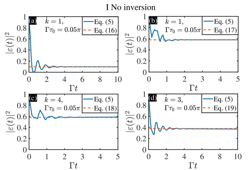
Figure 2: Static bound states for the giant atom with the number of coupling points $N=3$, the blue-solid and orange-dashed lines correspond to the numerical simulation in Eq. (5) and the analytical solutions with Eqs. (16)-(19), respectively. The parameters chosen are (a) $k=1,\omega_{0}\tau_{0}=2\pi,\Gamma\tau_{0}=0.05\pi$; (b) $k=1,\omega_{0}\tau_{0}=3\pi,\Gamma\tau_{0}=0.05\pi$; (c) $k=4,\omega_{0}\tau_{0}=2.6234\pi,\Gamma\tau_{0}=0.05\pi$; (d) $k=3,\omega_{0}\tau_{0}=1.6\pi,\Gamma\tau_{0}=0.05\pi$.

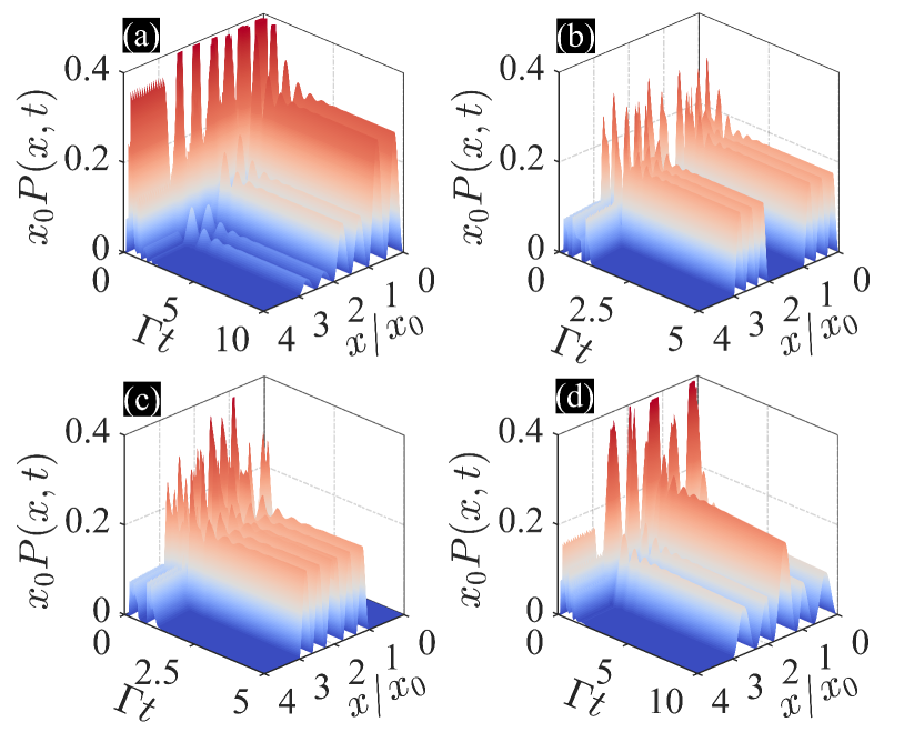
Figure 3: The figure shows the evolution of the field intensity $P(x,t)={\left|{\phi(x,t)}\right|^{2}}$ with time and position by solving Eq. (6) in the waveguide under four different conditions. The colors indicate the field intensity of the bound states. The parameters chosen are the same as those in Fig. 2.

In this section, we give the conditions for the generation of bound states and discuss whether these conditions can coexist. $s_{k}$ in Eq. (10) is pure imaginary when the real part of the complex frequency $s_{k}$ denoting the relaxation rate equals $0$. In this case, the corresponding mode is a bound state not decaying despite the dissipative environment. We seek the pure imaginary solution ${s_{k}}=-i{\omega_{k}}$ in Eq. (10), which can be satisfied when

$${s_{k}} =-i{\omega_{k}}=-i{\omega_{0}}=-i2k\pi/{\tau_{0}},$$ (11a)

$${s_{k}} =-i{\omega_{k}}=-i{\omega_{0}}=-i(2k+1)\pi/{\tau_{0}},$$ (11b)

and the corresponding bound state conditions are

$${\omega_{0}}{\tau_{0}} ={\omega_{k}}{\tau_{0}}=2k\pi,$$ (12a)

$${\omega_{0}}{\tau_{0}} ={\omega_{k}}{\tau_{0}}=(2k+1)\pi.$$ (12b)

In order to find more ${s_{k}}$ meeting Eq. (10), we divide Eq. (10) into real and imaginary parts respectively described through

$$\Gamma{\tau_{0}}{\csc^{2}}\left(\frac{{{\omega_{k}}{\tau_{0}}}}{2}\right){\sin^{2}}\left(\frac{{N{\omega_{k}}{\tau_{0}}}}{2}\right){\sin^{2}}\left[\frac{{\left(N+1\right){\omega_{k}}{\tau_{0}}}}{2}\right]=0\hfill,$$ (13)

$$\Gamma{\tau_{0}}\sin({\omega_{k}}{\tau_{0}})+2N\Gamma{\tau_{0}}\sin({\omega_{k}}{\tau_{0}})-2\Gamma{\tau_{0}}\sin(N{\omega_{k}}{\tau_{0}})$$

$$-2\Gamma{\tau_{0}}\sin\left[{(N+1){\omega_{k}}{\tau_{0}}}\right]+\Gamma{\tau_{0}}\sin\left[{(2N+1){\omega_{k}}{\tau_{0}}}\right]$$

$$-4({\omega_{k}}{\tau_{0}}-{\omega_{0}}{\tau_{0}})\left[{1-\cos({\omega_{k}}{\tau_{0}})}\right]=0,$$

which can be derived in Appendix B. Solving the two equations in Eq. (13) simultaneously, we obtain

$${s_{k}} =-i{\omega_{k}}=-i2k\pi/\left({N{\tau_{0}}}\right),$$ (14a)

$${s_{k}} =-i{\omega_{k}}=-i2k\pi/\left[{\left({N+1}\right){\tau_{0}}}\right],$$ (14b)

and the corresponding bound state conditions satisfy

$${\omega_{0}}{\tau_{0}} =\frac{{2k\pi}}{N}-\frac{1}{2}N\Gamma{\tau_{0}}\cot\left(\frac{{k\pi}}{N}\right),$$ (15a)

$${\omega_{0}}{\tau_{0}} =\frac{{2k\pi}}{{N+1}}-\frac{1}{2}\left(N+1\right)\Gamma{\tau_{0}}\cot\left(\frac{{k\pi}}{{N+1}}\right).$$ (15b)

Under the Markovian limit ($\Gamma{\tau_{0}}\to 0$), the bound state conditions (15a) and (15b) can be reduced to ${\omega_{0}}{\tau_{0}}=2k\pi/N$ and ${\omega_{0}}{\tau_{0}}=2k\pi/(N+1)$. However, in the non-Markovian regime with the large enough $\Gamma{\tau_{0}}$, the influence of the cotangent terms in Eqs. (15a) and (15b) can not be ignored. Solving the transcendental equation in Eq. (15a) or (15b) leads to two cases containing only one integer $k$ satisfying it or both two integers $k_{1}$ and $k_{2}$ meeting it, whose derivation can be found in Appendix C. To ensure the validity of the rotating-wave approximation, we need to guarantee $\left|{{\omega_{k}}-{\omega_{0}}}\right|/{\omega_{0}}\ll 1$, which is equivalent to $|N\Gamma\cot(k\pi/N)/(2\omega_{0})|\ll 1$ and $|(N+1)\Gamma\cot[k\pi/(N+1)]/(2\omega_{0})|\ll 1$ with $k\in{\mathbb{Z}^{+}}$ according to Eqs. (15a) and (15b).

Based on the number of bound states in the waveguide, we obtain three cases and summarize them as follows:

(i) One of the bound state conditions (12a), (12b), (15a), and (15b) is satisfied, and there is only one integer $k_{0}$ as its solution. In this case, there will be four situations given by Eqs. (16)-(19) with Eqs. (11) and (14) (see Sec. V for more details).

(ii) Two integer solutions $k_{1}$ and $k_{2}$ meet the bound state condition (15a) or (15b), which will induce two cases obtained by Eqs. (20) and (21) with Eq. (14) in Sec. V.

(iii) Eq. (12a) or (12b) is satisfied on the basis of meeting the case (ii), which leads to the existence of three integers $k_{0}$, $k_{1}$, and $k_{2}$ simultaneously. The corresponding four results determined by Eqs. (22), (23), (42), and (LABEL:D2) with Eqs. (11) and (14) will be studied in Sec. V and Appendix C.

Next, we discuss the dynamics and output field of the giant atom in detail.

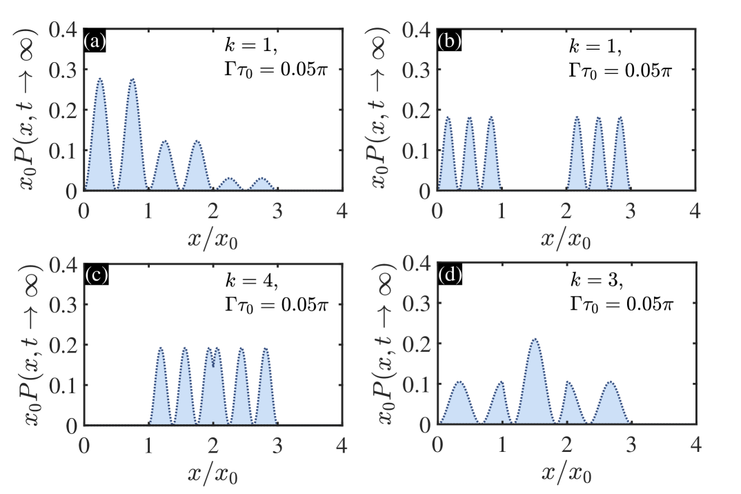
Figure 4: The field intensity distribution $P(x,t)$ in the waveguide at $t\rightarrow\infty$. The four cases shown by (a)-(d) correspond to Figs. 3(a)-3(d), where the blue-dotted line corresponds to the numerical simulation based on Eq. (6). The parameters chosen are the same as those in Fig. 3.

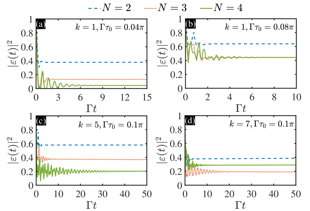
Figure 5: Probability amplitudes in Eq. (5) as function of time $t$ (in units of $\Gamma^{-1}$) when the number of coupling points $N$ is different. The blue-dashed, orange-dotted, and green-solid lines correspond to $N=2,N=3,N=4$, respectively. The other parameters chosen are (a) $k=1,\Gamma\tau_{0}=0.04\pi$; (b) $k=1,\Gamma\tau_{0}=0.08\pi$; (c) $k=5,\Gamma\tau_{0}=0.1\pi$; (d) $k=7,\Gamma\tau_{0}=0.1\pi$.

V Bound states in the semi-infinite waveguide

We study the non-Markovian dynamics in the three cases obtained from the discussion of the bound state conditions in Sec. IV. For the sake of clearness, we divide them into the static bound states with the no inversion of population, the periodic equal amplitude oscillation with two bound states, and the periodic non-equal amplitude oscillation with three bound states. In the following sections, we will discuss them and give the physical origins of the bound states formation.

V.1 No inversion of population

We consider the static bound state satisfying case (i) in Sec. IV, which means that the bound state in the waveguide has only one frequency. Substituting four $s_{k}$ in Eqs. (11) and (14) into Eq. (9), the long-time dynamics of the atomic excitation probability amplitude for four cases reads

$$\varepsilon(t) = \frac{1}{{1+\frac{\Gamma}{2}\sum\limits_{m,n=1}^{N}{\left[{-\left|{m-n}\right|{\tau_{0}}+\left({m+n}\right){\tau_{0}}}\right]}}}{e^{-i2k\pi t/{\tau_{0}}}},$$ (16)

$$\varepsilon(t) = \frac{1}{{1+\frac{\Gamma}{2}\sum\limits_{m,n=1}^{N}{\left[{-\left|{m-n}\right|{\tau_{0}}{{\left({-1}\right)}^{\left|{m-n}\right|}}+\left({m+n}\right){\tau_{0}}{{\left({-1}\right)}^{\left({m+n}\right)}}}\right]}}}{e^{-i(2k+1)\pi t/{\tau_{0}}}},$$ (17)

$$\varepsilon(t) = \frac{{2{{\sin}^{2}}({\omega_{k}}{\tau_{0}}/2)}}{{2{{\sin}^{2}}({\omega_{k}}{\tau_{0}}/2)+N\Gamma{\tau_{0}}}}{e^{-i2k\pi t/\left({N{\tau_{0}}}\right)}},$$ (18)

$$\varepsilon(t) = \frac{{2{{\sin}^{2}}({{\tilde{\omega}}_{k}}{\tau_{0}}/2)}}{{2{{\sin}^{2}}({{\tilde{\omega}}_{k}}{\tau_{0}}/2)+(N+1)\Gamma{\tau_{0}}}}{e^{-i2k\pi t/\left[{(N+1){\tau_{0}}}\right]}},$$ (19)

where ${\omega_{k}}=2k\pi/\left({N{\tau_{0}}}\right)$ and ${{\tilde{\omega}}_{k}}=2k\pi/\left[{(N+1){\tau_{0}}}\right]$.

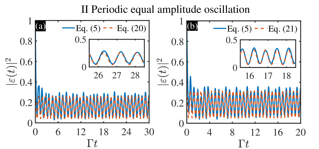
Figure 6: Periodic equal amplitude oscillating bound states in the waveguide for a giant atom with the number of coupling points $N=6$. The orange-dashed and blue-solid lines correspond to the analytical solutions in Eqs. (20) and (21) and numerical simulation of Eq. (5), respectively. The parameters chosen are (a) $k_{1}=23,k_{2}=26,\omega_{0}\tau_{0}=8.4167\pi,\Gamma\tau_{0}=0.1443\pi$; (b) $k_{1}=27,k_{2}=30,\omega_{0}\tau_{0}=8.3336\pi,\Gamma\tau_{0}=0.0852\pi$. $\omega_{k_{n}}$ in (a) and (b) are determined by Eqs. (14a) and (14b), respectively. The insets in the figure magnify the probability amplitudes.

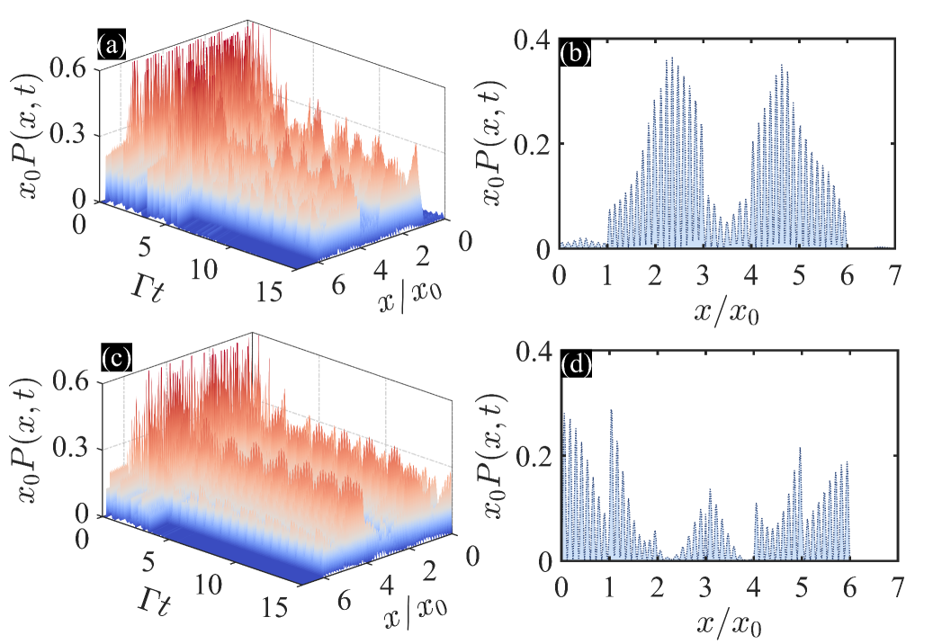
Figure 7: Plot of the field intensity function $P(x,t)$ solved by Eq. (6) as a function of $\Gamma t$ and $x/x_{0}$. (a) and (c) show the evolution of the field intensity in the waveguide corresponding to Fig. 6. The colors in (a) and (c) show the field intensity of the bound states. (b) and (d) denote the field intensity distribution $P(x,t)$ in the waveguide at fixed parameter $t=15/\Gamma$ corresponding to (a) and (c), respectively, where the blue-dotted line is the numerical simulation based on Eq. (6). The other parameters are the same as those in Fig. 6.

To compare the analytical solutions given by Eqs. (16)-(19) with the numerical simulation of Eq. (5), we plot the atomic excitation probability with $N=3$ as a function of time $t$ (in units of $\Gamma^{-1}$) in Fig. 2. The blue-solid and orange-dashed lines indicate the numerical and analytical results, respectively. We find that the analytical expressions show good agreement with those obtained by the numerical simulations with different parameters. In Fig. 2, the atomic excitation probabilities ${\left|{\varepsilon(t)}\right|^{2}}$ in the four cases finally hold a nonzero steady value after a long time, which means that the photon is captured and forms a bound state. This originates from the transferring of the photon in multiple coupling points and reflecting via the semi-infinite waveguide.

To observe how the bound state is formed, we take the field intensity function $P(x,t)$ as a function of the time $t$ (in units of $\Gamma^{-1}$) and the position $x$ (in units of $x_{0}^{-1}$). The time evolution of the field intensity function for the four different bound states with the number of coupling points $N=3$ is shown in Fig. 3. We observe that the field intensity outside the last coupling point ($x>3x_{0}$) disappears with time, while the field intensity at $x<3x_{0}$ forms a steady state, where a static bound state has been formed in the waveguide. In Fig. 4, we plot the long-time field intensity distribution corresponding to Fig. 3, where the blue-dashed line denotes the numerical simulation given by Eq. (6). In Fig. 4, the field intensities in the above four cases are distributed between the last coupling point and the mirror at the endpoint of the semi-infinite waveguide with $\Gamma t\to\infty$.

The variation of the atomic excitation probability $|\varepsilon(t)|^{2}$ with respect to the $\Gamma t$ for different number coupling points $N$ is plotted in Fig. 5. We find that the atomic excitation probability is a steady value although it changes with the number of coupling points. This means that the static bound states with different probabilities can be got through tuning the number of coupling points $N$.

V.2 Periodic equal amplitude oscillating bound states

When case (ii) in Sec. IV is met, two bound states with frequencies $\omega_{k_{1}}$ and $\omega_{k_{2}}$ exist simultaneously in the system. Substituting ${s_{k}}=\{-i2k\pi/\left({N{\tau_{0}}}\right),-i2k\pi/\left[{(N+1){\tau_{0}}}\right]\}$ obtained by Eq. (14) into Eq. (9), the long-time atomic excitation probability amplitudes are given by

$$\varepsilon(t)= \frac{{2{{\sin}^{2}}({\omega_{{k_{1}}}}{\tau_{0}}/2)}}{{2{{\sin}^{2}}({\omega_{{k_{1}}}}{\tau_{0}}/2)+N\Gamma{\tau_{0}}}}{e^{-i2{k_{1}}\pi t/\left({N{\tau_{0}}}\right)}}$$ (20)

$$+\frac{{2{{\sin}^{2}}({\omega_{{k_{2}}}}{\tau_{0}}/2)}}{{2{{\sin}^{2}}({\omega_{{k_{2}}}}{\tau_{0}}/2)+N\Gamma{\tau_{0}}}}{e^{-i2{k_{2}}\pi t/\left({N{\tau_{0}}}\right)}},$$

where ${\omega_{{k_{n}}}}=2{k_{n}}\pi/\left({N{\tau_{0}}}\right)~{}(n=1,~{}2)$, and

$$\varepsilon(t)= \frac{{2{{\sin}^{2}}({\omega_{{k_{1}}}}{\tau_{0}}/2)}}{{2{{\sin}^{2}}({\omega_{{k_{1}}}}{\tau_{0}}/2)+(N+1)\Gamma{\tau_{0}}}}{e^{-i2{k_{1}}\pi t/\left[{(N+1){\tau_{0}}}\right]}}$$ (21)

$$+\frac{{2{{\sin}^{2}}({\omega_{{k_{2}}}}{\tau_{0}}/2)}}{{2{{\sin}^{2}}({\omega_{{k_{2}}}}{\tau_{0}}/2)+(N+1)\Gamma{\tau_{0}}}}{e^{-i2{k_{2}}\pi t/\left[{(N+1){\tau_{0}}}\right]}},$$

with ${\omega_{{k_{n}}}}=2{k_{n}}\pi/\left[{(N+1){\tau_{0}}}\right]~{}(n=1,~{}2)$.

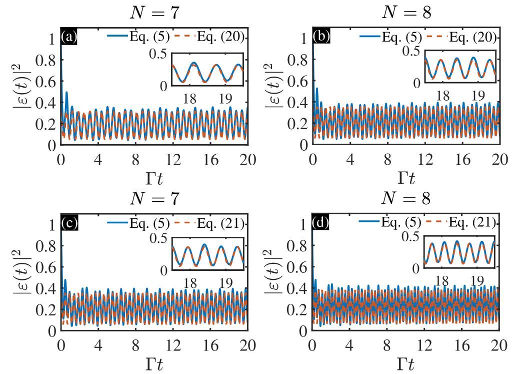
Figure 8: The influence of different number of coupling points $N$ on the equal amplitude oscillating bound states for the giant atom. The orange-dashed and blue-solid lines correspond to the analytical solutions in Eqs. (20) and (21) and numerical simulations based on Eq. (5), respectively. The parameters chosen are (a) $N=7,k_{1}=27,k_{2}=30,\omega_{0}\tau_{0}=8.3336\pi,\Gamma\tau_{0}=0.0852\pi$; (b) $N=8,k_{1}=31,k_{2}=34,\omega_{0}\tau_{0}=8.2803\pi,\Gamma\tau_{0}=0.0549\pi$; (c) $N=7,k_{1}=31,k_{2}=34,\omega_{0}\tau_{0}=8.2803\pi,\Gamma\tau_{0}=0.0549\pi$; (d) $N=8,k_{1}=35,k_{2}=38,\omega_{0}\tau_{0}=8.2428\pi,\Gamma\tau_{0}=0.0376\pi$. $\omega_{k_{n}}$ in (a)-(b) and (c)-(d) are determined by Eqs. (14a) and (14b), respectively.

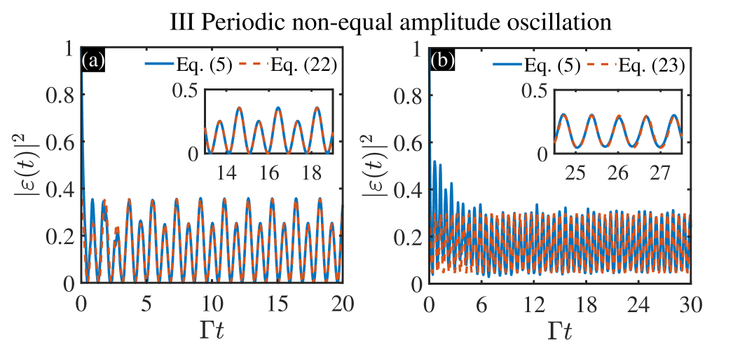
Figure 9: Non-equal amplitude oscillating bound states of a giant atom. The orange-dashed and blue-solid lines correspond to the analytical solutions in Eqs. (22) and (23) and numerical simulation solved by Eq. (5), respectively. The parameters chosen are (a) $N=5,k_{0}=4,k_{1}=19,k_{2}=21,\omega_{0}\tau_{0}=8\pi,\Gamma\tau_{0}=0.1162\pi$; (b) $N=8,k_{0}=8,k_{1}=63,k_{2}=73,\omega_{0}\tau_{0}=17\pi,\Gamma\tau_{0}=0.1294\pi$. $\omega_{k_{n}}$ in (a) and (b) are determined by Eq. (14a).

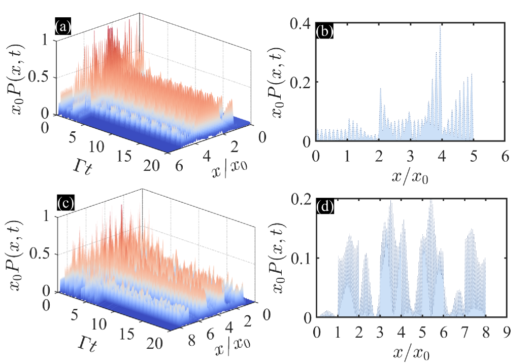
Figure 10: The field strength $P(x,t)={\left|{\phi(x,t)}\right|^{2}}$ as a function of $\Gamma t$ and $x/x_{0}$ based on Eq. (6). (a) and (c) show the time evolution of the field intensity $P(x,t)$ in the waveguide corresponding to Figs. 9(a) and 9(b), where the parameters $k_{0},k_{1},$ and $k_{2}$ are the same as those in Fig. 9. The colors in (a) and (c) describe the field intensity of the bound states. For clarity, (b) and (d) show the distribution of $P(x,t)$ in the waveguide at $t=20/\Gamma$, which respectively correspond to (a) and (c). The blue-dotted line corresponds to the numerical simulation of Eq. (6).

In this case, two integers $k_{1}$ and $k_{2}$ that satisfy transcendental equation (15a) or (15b) can be found. The atomic excitation probability ${\left|{\varepsilon(t)}\right|^{2}}$ is the superposition of the bound states with different frequencies ${\omega_{{k_{1}}}}$ and ${\omega_{{k_{2}}}}$. In Appendix C, we give $\omega_{0}\tau_{0}$ and $\Gamma\tau_{0}$ for the existence of two bound states. The long-time dynamics in Eq. (20) is consistent with that given in Refs. Guo0430142020 ; Lim0237162023 . However, in addition to Eq. (20), another solution in Eq. (21) can be sought out, which is significantly different from that in Refs. Guo0430142020 ; Lim0237162023 and induced by the reflection of the semi-infinite waveguide and time delay between multiple coupling points. This indicates that the atomic excitation probability can be manipulated due to the existence of the mirror in the semi-infinite waveguide without changing the number of coupling points.

We plot the numerical result based on Eq. (5) and analytical results in Eqs. (20) and (21) for the atomic excitation probability denoted by the blue-solid and orange-dashed lines in Fig. 6. In principle, we can get the atomic excitation probability ${\left|{\varepsilon(t)}\right|^{2}}$ as a function of $\Gamma t$ with any $N$ in the above two cases. We take the number of coupling points $N=6$ to exhibit typical features of the atomic excitation probability. Interestingly, the quantum interference effects between multiple coupling points and the semi-infinite waveguide lead to the approximate periodic oscillation behaviors of the dynamics, and the amplitudes of periodic oscillations do not decrease with time.

Similar to the case of the static bound state, we study the dependence of the field intensity function $P(x,t)$ on $x/x_{0}$ and $\Gamma t$ in Fig. 7. We show the time evolution of the field intensity function $P(x,t)$ at $x/x_{0}$ in Figs. 7(a) and 7(c). The energy is bound between $0\sim 6x_{0}$ with the position of the last coupling point as the boundary, while the energy outside the last coupling point disappears with time. The field intensity oscillates persistently after a long time due to the existence of bound states with two different frequencies in the waveguide. In Figs. 7(b) and 7(d), we show the field intensity distribution calculated by Eq. (6) at $\Gamma t=15$ corresponding to Figs. 7(a) and 7(c).

In order to understand the influence of the number of coupling points on the atomic excitation probability, the dynamics with different number of coupling points ($N=7,8$) in two cases given by Eqs. (20) and (21) is shown in Fig 8. The amplitude and frequency of the atomic excitation probability change with the number of coupling points.

V.3 Periodic non-equal amplitude oscillating bound states

We study the coexistence of bound states with three different frequencies ${\omega_{{k_{0}}}}$, ${\omega_{{k_{1}}}}$, and ${\omega_{{k_{2}}}}$ described by case (iii) in Sec. IV. In this section, we analyze the situation that Eq. (12a) or (12b) is satisfied when meeting Eq. (15a). The other cases of bound states with three frequencies are discussed in Appendix D. With Eqs. (11) and (14), the atomic dynamics in Eq. (9) becomes

$$\varepsilon(t) = \frac{1}{{1+\frac{\Gamma}{2}\sum\limits_{m,n=1}^{N}{\left[{-\left|{m-n}\right|{\tau_{0}}+\left({m+n}\right){\tau_{0}}}\right]}}}{e^{-i2{k_{0}}\pi t/{\tau_{0}}}}$$ (22)

$$+\frac{{2{{\sin}^{2}}({\omega_{{k_{1}}}}{\tau_{0}}/2)}}{{2{{\sin}^{2}}({\omega_{{k_{1}}}}{\tau_{0}}/2)+N\Gamma{\tau_{0}}}}{e^{-i2{k_{1}}\pi t/\left({N{\tau_{0}}}\right)}}+\frac{{2{{\sin}^{2}}({\omega_{{k_{2}}}}{\tau_{0}}/2)}}{{2{{\sin}^{2}}({\omega_{{k_{2}}}}{\tau_{0}}/2)+N\Gamma{\tau_{0}}}}{e^{-i2{k_{2}}\pi t/\left({N{\tau_{0}}}\right)}},$$

$$\varepsilon(t) = \frac{1}{{1+\frac{\Gamma}{2}\sum\limits_{m,n=1}^{N}{\left[{-\left|{m-n}\right|{\tau_{0}}{{\left({-1}\right)}^{\left|{m-n}\right|}}+\left({m+n}\right){\tau_{0}}{{\left({-1}\right)}^{\left({m+n}\right)}}}\right]}}}{e^{-i(2{k_{0}}+1)\pi t/{\tau_{0}}}}$$ (23)

$$+\frac{{2{{\sin}^{2}}({\omega_{{k_{1}}}}{\tau_{0}}/2)}}{{2{{\sin}^{2}}({\omega_{{k_{1}}}}{\tau_{0}}/2)+N\Gamma{\tau_{0}}}}{e^{-i2{k_{1}}\pi t/\left({N{\tau_{0}}}\right)}}+\frac{{2{{\sin}^{2}}({\omega_{{k_{2}}}}{\tau_{0}}/2)}}{{2{{\sin}^{2}}({\omega_{{k_{2}}}}{\tau_{0}}/2)+N\Gamma{\tau_{0}}}}{e^{-i2{k_{2}}\pi t/\left({N{\tau_{0}}}\right)}},$$

where ${\omega_{k_{n}}}(n=1,2)$ in Eqs. (22) and (23) are given by Eqs. (40) and (41), respectively. The derivation details of ${\omega_{k_{n}}}$ can be found in Appendix C.

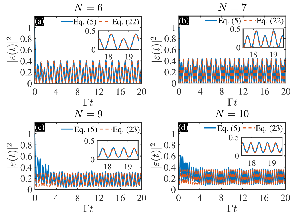
Figure 11: The influence of different number of coupling points $N$ on the non-equal amplitude oscillating bound states for the giant atom. The orange-dashed and blue-solid lines respectively correspond to the analytical solutions in Eqs. (22) and (23) and the numerical simulation of Eq. (5). The parameters chosen are (a) $N=6,k_{0}=4,k_{1}=23,k_{2}=25,\omega_{0}\tau_{0}=8\pi,\Gamma\tau_{0}=0.0642\pi$; (b) $N=7,k_{0}=4,k_{1}=27,k_{2}=29,\omega_{0}\tau_{0}=8\pi,\Gamma\tau_{0}=0.0393\pi$; (c) $N=9,k_{0}=8,k_{1}=71,k_{2}=82,\omega_{0}\tau_{0}=17\pi,\Gamma\tau_{0}=0.0989\pi$; (d) $N=10,k_{0}=8,k_{1}=79,k_{2}=91,\omega_{0}\tau_{0}=17\pi,\Gamma\tau_{0}=0.078\pi$. $\omega_{k_{n}}$ in (a)-(d) are determined by Eq. (14a).

The dynamics with three coexisting bound states ${\omega_{{k_{0}}}}$, ${\omega_{{k_{1}}}}$, and ${\omega_{{k_{2}}}}$ in Eqs. (22) and (23) stems from the interaction of the photon through a semi-infinite waveguide and multiple coupling points, which is completely different from that in Refs. Guo0430142020 ; Lim0237162023 , where the coexistence of at most two bound modes is achieved. The dynamics of the atomic excitation probability amplitude $\varepsilon(t)$ determined by Eqs. (22) and (23) in a semi-infinite waveguide is the superposition of three bound states with different frequencies in the long-time limit after the disappearance of all dissipative modes.

Figure 9 shows the excitation dynamics of the giant atom, where the blue-solid and orange-dashed lines denote the numerical simulation of Eq. (5) and analytical results based on Eqs. (22) and (23), respectively. We find that atomic excitation dynamics of bound states with three frequencies exhibits non-equal amplitude persistent oscillation, where the differences between the dynamical characteristics in Figs. 9(a) and 9(b) are explained in Appendix D. We use the field intensity function $P(x,t)$ as a function of $\Gamma t$ and $x/x_{0}$ and show the field intensity distribution in Fig. 10. Consistent with the static and equal amplitude oscillating bound states, the field intensity is bound between the mirror and the last coupling point. For clearer observation, we plot the field intensity distribution in the waveguide with the fixed parameter $\Gamma t=20$ corresponding to Figs. 10(a) and 10(c), as shown in Figs. 10(b) and 10(d). We find that the field intensity distribution outside the last coupling point is $0$, which means that a perfect bound state is formed in the waveguide.

Figure 12: In order to understand the influence of reflectivity $R$ on the bound states, we plot the atomic excitation probability with different reflectivity $R$. The blue-dotted line denotes the ideal case, where the mirror has a perfect reflectivity $R=1$. The green-dashed and orange-solid lines respectively correspond to the case of no mirror $(R=0)$ and general case $(R=0.9)$. The atomic excitation probability ${\left|{\varepsilon(t)}\right|^{2}}$ is plotted by solving Eq. (24). The static bound states, equal amplitude oscillating bound states and non-equal amplitude oscillating bound states correspond to (a)-(d), (e)-(f), and (g)-(h), respectively. The parameters chosen are $\Gamma_{ext}=0$ and $\lambda(t)=0$ without considering the influence of the dephasing process and external decay.

Finally, we plot the dynamics of the giant atom with different numbers of coupling points in Fig. 11. The probability of the giant atom in the excited state depends on the number of coupling points. Tuning the number of coupling points can change the frequency and amplitude of atomic excitation probability.

VI extension to general model

We focus on the non-Markovian dynamics of a two-level giant atom in a semi-infinite waveguide, where the waveguide is terminated by a perfect mirror with reflectivity $R=1$ at $x=0$. Considering the realistic experimental environment, we make some changes to the model to explain the detrimental factors.

Firstly, for the waveguide in the experiment, the reflectivity $R$ of the mirror is usually less than $1$. The complex probability amplitude $-r$ for backward reflection of the mirror satisfies ${|r|^{2}}=R$. Solving the one-dimensional scattering problem yields $r=R+i\sqrt{R(1-R)}$. The delay term in Eq. (5) suggests the replacement $\frac{\Gamma}{2}\sum_{m,n=1}^{N}{\varepsilon\left[{t-(m+n){\tau_{0}}}\right]\Theta\left[{t-(m+n){\tau_{0}}}\right]}\to\frac{\Gamma}{2}r\sum_{m,n=1}^{N}{\varepsilon\left[{t-(m+n){\tau_{0}}}\right]\Theta\left[{t-(m+n){\tau_{0}}}\right]}$ since the giant atom will reinteract only with the reflected part of the light. In addition to the emissions of the atomic excited state into waveguide modes at rate ${\Gamma}$, we allow for an extra atomic coupling to a reservoir of external nonaccessible modes at a rate ${\Gamma_{ext}}$. When the external mode does not decay to the waveguide mode, the total effective dissipation rate of the excited atom is ${\Gamma_{tot}}=\Gamma+{\Gamma_{ext}}$. It simply amounts to adding a term $-{{N{\Gamma_{ext}}}}\varepsilon(t)/2$ on the right-hand side of Eq. (5). Finally, we add a small white-noise stochastic term $\omega(t)={\omega_{0}}+\lambda(t)$ to the excited state frequency to introduce (inhomogeneous) phase noise on the giant atom. Here the Gaussian distributed stochastic term $\lambda(t)$ is characterized by its zero mean ${\left\langle{\lambda(t)}\right\rangle_{t}}=0$ and the noise correlation function $\left\langle{\lambda(t)\lambda(t^{\prime})}\right\rangle=2\delta\omega\delta(t-t^{\prime})$ ($\left\langle{...}\right\rangle$ stands for the ensemble average) Chenu1404032017 ; Khripkov0216062011 , where $\delta\omega$ denotes the associated dephasing rate.

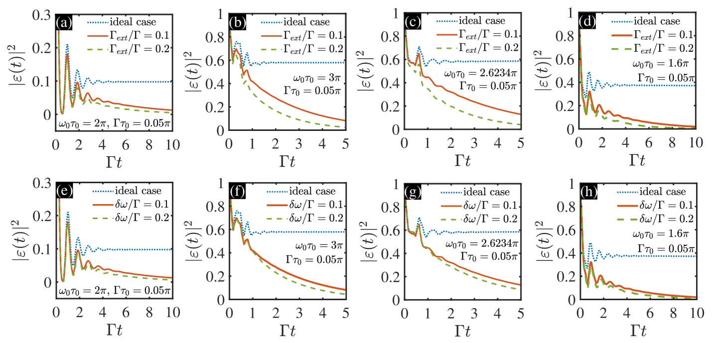
Figure 13: The influence of the external reservoir decay rate $\Gamma_{ext}$ and dephasing rate $\delta\omega$ on the static bound states with the number of coupling points $N=3$. The blue-dotted line represents the ideal case ($R=1,\delta\omega=0,\Gamma_{ext}=0$). For (a)-(d), we fix $R=0.98$ and $\delta\omega=0.1\Gamma$ and vary the ratio between $\Gamma_{ext}$ and $\Gamma$ with keeping $\Gamma$ fixed. For (e)-(h), we remain $R=0.98$ and $\Gamma_{ext}=0.1\Gamma$, and change the dephasing rate $\delta\omega$.

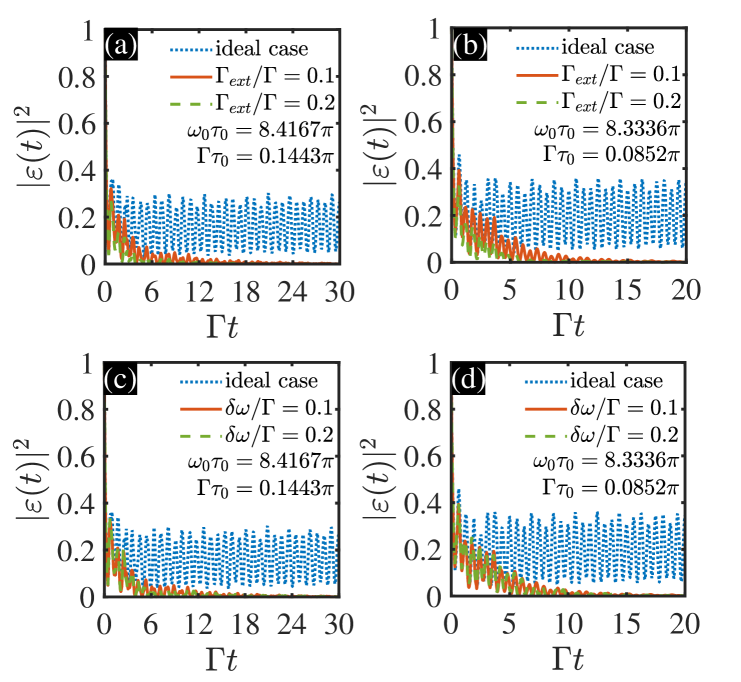
Figure 14: Influences of the different dephasing processes and external decay on the equal amplitude oscillating bound states for a giant atom with the number of coupling points $N=6$. The atomic excitation probability ${\left|{\varepsilon(t)}\right|^{2}}$ is plotted by solving Eq. (24). (a)-(b) show the influences of different external reservoir decay rates $\Gamma_{ext}$ on the atomic excitation probability with the fixed parameter $R=0.98$ and $\delta\omega=0.1\Gamma$. The orange-solid and green-dashed lines respectively correspond to $\Gamma_{ext}=0.1\Gamma$ and $\Gamma_{ext}=0.2\Gamma$. In (c)-(d), we take $R=0.98$ and $\Gamma_{ext}=0.1\Gamma$, where the orange-solid and green-dashed lines correspond to $\delta\omega=0.1\Gamma$ and $\delta\omega=0.2\Gamma$, respectively. The blue-dotted line corresponds to the ideal case with $R=1$, $\Gamma_{ext}=0$, and $\delta\omega=0$.

In conclusion, Eq. (5) involved in the dephasing processes becomes

$$\dot{\varepsilon}(t)= -i\left[{\omega_{0}}+\lambda(t)\right]\varepsilon(t)-\frac{{N{\Gamma_{ext}}}}{2}\varepsilon(t)$$ (24)

$$-\frac{\Gamma}{2}\sum\limits_{m,n=1}^{N}{\varepsilon\left(t-\left|{m-n}\right|{\tau_{0}}\right)\Theta\left(t-\left|{m-n}\right|{\tau_{0}}\right)}$$

$$+\frac{\Gamma}{2}r\sum\limits_{m,n=1}^{N}{\varepsilon\left[{t-\left(m+n\right){\tau_{0}}}\right]\Theta\left[{t-\left(m+n\right){\tau_{0}}}\right]}.$$

When we adjust the reflectivity $R$ of the mirror at the end of the semi-infinite waveguide, the atomic excitation probabilities of the static, equal amplitude oscillating and non-equal amplitude oscillating bound states are shown in Fig. 12. Except for Figs. 12(c), 12(e), 12(g), and 12(i) obtained by Eqs. (18), (20), (22), and (23), the atomic excitation probabilities decay significantly when the reflectivity $R=0$, which denotes that the formation of the bound states except for these four cases strongly depend on the existence of the semi-infinite waveguide. The results got without considering the presence of a mirror $(R=0)$ are equivalent to those through a two-level giant atom interacting with a one-dimensional infinite waveguide.

For practical giant atom waveguide systems, in addition to dephasing, we also allow the giant atom to couple to a reservoir of external inaccessible modes and the semi-infinite waveguide of non-ideal mirrors. In Figs. 13(a)-13(d), we show the atomic excitation probabilities for static bound states with $R=0.98$ and $\delta\omega=0.1\Gamma$. We give the different external reservoir decay rates ${\Gamma_{ext}}=\{{0.1\Gamma,0.2\Gamma}\}$ and compare them with the ideal case ($R=1$, ${\Gamma_{ext}}=0$, $\delta\omega=0$). The atomic probability decreases as the decay rate ${\Gamma_{ext}}$ increases, which indicates that the decay of the external inaccessible mode inhibits the formation of bound states. We plot the atomic probabilities with different dephasing rates $\delta\omega=\{{0.1\Gamma,0.2\Gamma}\}$ and compare them with the ideal case ($R=1$, ${\Gamma_{ext}}=0$, $\delta\omega=0$) in Figs. 13(e)-13(h), where the other parameters chosen are $R=0.98$ and ${\Gamma_{ext}}=0.1\Gamma$. The results show the inhibition effect of dephasing rate on probability, which is more obvious when the dephasing rate becomes larger. Figs. 14 and 15 correspond to the influence of dephasing and external reservoir decay rates on the equal amplitude and non-equal amplitude oscillating bound states. Consistent with the static bound states, the atomic excitation probabilities decay rapidly when the dephasing and relaxation rates increase.

VII multiple giant atoms are coupled to a one-dimensional semi-infinite waveguide

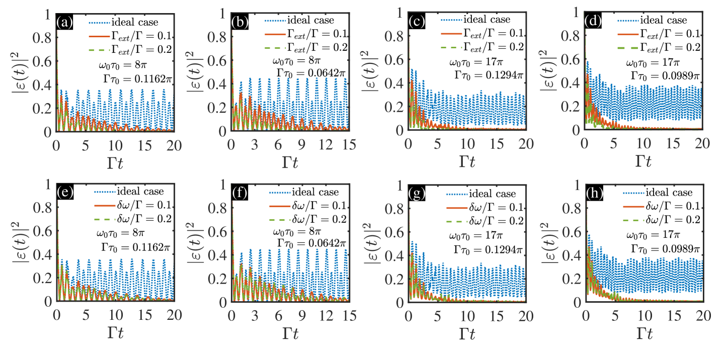
Figure 15: The figure shows the influences of the external reservoir decay rate $\Gamma_{ext}$ and dephasing rate $\delta\omega$ on the non-equal amplitude oscillating bound states. The blue-dotted line denotes the ideal case ($R=1,\delta\omega=0,\Gamma_{ext}=0$). The orange-solid and green-dashed lines respectively correspond to $\Gamma_{ext}=0.1\Gamma$ and $\Gamma_{ext}=0.2\Gamma$ in (a)-(d), while those in (e)-(h) respectively correspond to $\delta\omega=0.1\Gamma$ and $\delta\omega=0.2\Gamma$. The other parameters chosen are (a)-(d) $R=0.98,\delta\omega=0.1\Gamma$; (e)-(h) $R=0.98,\Gamma_{ext}=0.1\Gamma$.

,

We generalize the above results to a more general model involving $Q$ noninteracting two-level giant atoms coupled to a one-dimensional semi-infinite waveguide, where ground state $\left|g\right\rangle$ and excited state $\left|e\right\rangle$ of the $q$th atom are separated in frequency by $\omega_{q,0}~{}(q=1,2,...,Q)$. In Fig. 16, $Q$ giant atoms interact with a one-dimensional semi-infinite waveguide through $\sum_{q=1}^{Q}{{N_{q}}}$ coupling points, where $N_{q}$ denotes the number of coupling points for the $q$th giant atom. The distance between any adjacent coupling points is the same as that between the mirror and the first coupling point, both of which are $x_{0}$. $l_{q}$ denotes the sum of the number of all coupling points before the first coupling point of the $q$th giant atom, which is expressed as $l_{q}=\sum_{q^{\prime}=1}^{q-1}{{N_{q^{\prime}}}}$. The total Hamiltonian of the system in the rotating-wave approximation is

$${\hat{H}_{Q}}= \sum\limits_{q=1}^{Q}{{\omega_{q,0}}}{|e\rangle_{qq}}\langle e|+\int_{0}^{{k_{c}}}{dk}{\Omega_{k}}\hat{a}_{k}^{\dagger}{{\hat{a}}_{k}}$$ (25)

$$+\sum\limits_{q=1}^{Q}{\sum\limits_{m=l_{q}+1}^{l_{q}+{N_{q}}}{\int_{0}^{{k_{c}}}{dk}{({g_{km}}\hat{a}_{k}^{\dagger}{\sigma_{q}}_{-}+{g_{km}^{*}}{{\hat{a}}_{k}}{\sigma_{q}}_{+})}}},$$

where ${\sigma_{q}}_{+}$ and ${\sigma_{q}}_{-}$ are raising and lowering operators of the $q$th giant atom. The first and second terms of Eq. (25) describe the free Hamiltonian of $Q$ giant atoms and the one-dimensional semi-infinite waveguide, where the frequency of the $q$th atom is denoted by ${\omega_{q,0}}={\omega_{0}}+{\delta_{q}}$. The last term of Eq. (25) results from the interaction between the $q$th giant atom and semi-infinite waveguide. We assume that the initial state is prepared in $|{\psi(0)}\rangle=\sum_{q=1}^{Q}{{\varepsilon_{q}}(0)}|{{e_{q}},0}\rangle$, where $|{{e_{q}},0}\rangle$ denotes that the $q$th giant atom is on the excited state $|e\rangle$ with the probability amplitude ${\varepsilon_{q}}(0)$, but simultaneously all the modes of the waveguide are all in the vacuum state. Schrödinger equation drives the initial state $|{\psi(0)}\rangle$ as

$$\left|{\psi(t)}\right\rangle=\sum\limits_{q=1}^{Q}{{\varepsilon_{q}}(t)}\left|{{e_{q}},0}\right\rangle+\int{dk\varphi(k,t)}\hat{a}_{k}^{\dagger}\left|{G,0}\right\rangle,$$ (26)

with $\left|{{e_{q}},0}\right\rangle={\left|g\right\rangle_{1}}\otimes{\left|g\right\rangle_{2}}\otimes\cdots{\left|e\right\rangle_{q}}\otimes\cdots{\left|g\right\rangle_{Q}}\otimes\left|0\right\rangle$ and $\left|{G,0}\right\rangle={\left|g\right\rangle_{1}}\otimes{\left|g\right\rangle_{2}}\otimes\cdots{\left|g\right\rangle_{q}}\otimes\cdots{\left|g\right\rangle_{Q}}\otimes\left|0\right\rangle.$ Substituting Eqs. (25) and (26) into Schrödinger equation, we obtain the probability amplitudes

$${{\dot{\varepsilon}}_{q}}(t) = -i{\omega_{q,0}}{\varepsilon_{q}}(t)-i\sum\limits_{m=l_{q}+1}^{l_{q}+{N_{q}}}{\int{dk{g_{km}^{*}}\varphi(k,t)}},$$ (27)

$$\dot{\varphi}(k,t) = -i{\Omega_{k}}\varphi(k,t)-i\sum\limits_{q=1}^{Q}{\sum\limits_{m=l_{q}+1}^{l_{q}+{N_{q}}}{g_{km}{\varepsilon_{q}}(t)}}.$$ (28)

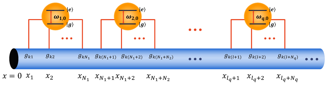
Figure 16: One-dimensional semi-infinite waveguide coupled to an array of noninteracting two-level giant atoms through $\sum_{q=1}^{Q}{{N_{q}}}$ coupling points with coupling coefficient $g_{km}$, where $N_{q}$ is the number of coupling points for the $q$th giant atom. The ground state $|g\rangle$ and the excited state $|e\rangle$ of the $q\mathrm{th}$ atom are separated in frequency by $\omega_{q,0}~{}(q=1,2,...,Q)$. $l_{q}$ denotes the sum of the number of all coupling points before the first coupling point of the $q$th giant atom, which is written as $l_{q}=\sum_{q^{\prime}=1}^{q-1}{{N_{q^{\prime}}}}$. The distance between any two adjacent coupling points is $x_{0}$, which is equal to that between the mirror and the first coupling point.

Integrating Eq. (28) with coupling coefficient ${g_{km}}=\sqrt{\Gamma v/\pi}\sin(km{x_{0}})$ results in

$$\varphi(k,t)=\frac{1}{i}\int_{0}^{t}{\sum\limits_{q=1}^{Q}{\sum\limits_{m=l_{q}+1}^{l_{q}+{N_{q}}}{\sqrt{\frac{{\Gamma v}}{\pi}}\sin(km{x_{0}}){\varepsilon_{q}}(s)}}{e^{-i{\Omega_{k}}\left({t-s}\right)}}ds}.$$ (29)

With Eq. (29), the probability amplitude in Eq. (27) becomes

$$\dot{\varepsilon}_{q}(t)= -i\omega_{q,0}\varepsilon_{q}(t)-i\delta_{q}\varepsilon_{q}(t)$$ (30)

$$-\frac{\Gamma}{2}\sum_{q=1}^{Q}\sum_{m,n=l_{q}+1}^{l_{q}+{N_{q}}}\varepsilon_{q}(t-|m-n|\tau_{0})$$

$$\times\Theta(t-|m-n|\tau_{0})$$

$$+\frac{\Gamma}{2}\sum_{q=1}^{Q}\sum_{m,n=l_{q}+1}^{l_{q}+{N_{q}}}\varepsilon_{q}[t-(m+n)\tau_{0}]$$

$$\times\Theta[t-(m+n)\tau_{0}].$$

Solving the set of time-delay differential equations in Eq. (30), we can get complete information about the $Q$ noninteracting two-level giant atoms. Interactions between any two or more giant atoms caused by the semi-infinite waveguide generally exist, which leads to quantum correlations between different giant atoms. The result of Eq. (30) is reduced to that in Eq. (5) when $Q=1$. It can be predicted that when $Q\neq 1$, there will be more modes of bound states in the waveguide simultaneously, which provides a positive way for us to control the coupled giant atoms through engineering the structured environment.

VIII conclusions and discussions

In this paper, we have investigated the non-Markovian dynamics in the spontaneous emission of a two-level giant atom interacting with a one-dimensional semi-infinite waveguide. We derived the analytical solutions for the atomic probability amplitude by Laplace transform, which show non-exponential dissipations due to the photon transferring between multiple coupling points and being reabsorbed after it is reflected by the semi-infinite waveguide. We discussed the conditions and origins for the formation of bound states and obtained three different bound states. According to the number of bound states in the waveguide, the bound states are divided into static case with one bound state, equal amplitude oscillation with two bound states, and non-equal amplitude oscillation with three bound states. The equal and non-equal amplitude oscillating bound states show the period oscillation behavior for the system, which can arise from the quantum interference effects between the multiple coupling points and semi-infinite waveguide. The oscillating bound states with multiple bound states provide a way for us to store and manipulate more complex quantum information. We assessed that the formation of bound states can be restricted in the presence of dissipation into unwanted modes and dephasing of the giant atom. Finally, we further expanded our analysis to a more general quantum system containing many noninteracting giant atoms interacting with a semi-infinite waveguide through multiple coupling points.

The study of non-Markovian dynamics in two-level giant atoms coupled to a one-dimensional semi-infinite waveguide may open up a way to better understand non-Markovian quantum networks and quantum communications. Moreover, compared to previous models, the obtained set of delay differential equations for the giant atom might pave the way to better understand the non-Markovian dynamics of many giant atoms coupled to a semi-infinite waveguide. As a prospect, we can further study anisotropic non-rotating wave two-level giant atomic systems through applying the method in Refs. Shi1536022018 ; Lo0638072018 ; Shen0237072022 ; Shen0238562018 ; Xie0210462014 ; Chen0437082021 ; Rodriguez0466082008 ; Nakajima43631955 ; Frohlich8451950 ; Frohlich2911952 ; Lu0543022007 and driven three-level giant atomic systems in rotating-wave approximation, which are respectively described by

$${{\hat{H}}_{2LS}}= {\omega_{e}}|e\rangle\langle e|+\int_{0}^{{k_{c}}}{dk}{\Omega_{k}}\hat{a}_{k}^{\dagger}{{\hat{a}}_{k}}+\sum\limits_{m}{\int_{0}^{{k_{c}}}{dk}}$$ (31)

$$\cdot[{a_{km}}({\hat{a}_{k}^{\dagger}{\sigma_{-}}+{{\hat{a}}_{k}}{\sigma_{+}}})+{b_{km}}({\hat{a}_{k}^{\dagger}{\sigma_{+}}+{{\hat{a}}_{k}}{\sigma_{-}}})],$$

$${{\hat{H}}_{3LS}}= {\omega_{x}}|x\rangle\langle x|+{\omega_{e}}|e\rangle\langle e|+\int_{0}^{{k_{c}}}{dk}$$

$$\cdot{\Omega_{k}}\hat{a}_{k}^{\dagger}{{\hat{a}}_{k}}+\tilde{\Omega}_{3LS}{e^{i{\omega_{l}}t}}{\sigma_{ex}}+\tilde{\Omega}_{3LS}{e^{-i{\omega_{l}}t}}{\sigma_{xe}}$$

$$+\sum\limits_{n}{\int_{0}^{{k_{c}}}{dk}{g_{kn}}(\hat{a}_{k}^{\dagger}{\sigma_{gx}}+{{\hat{a}}_{k}}{\sigma_{xg}})},$$

where $a_{km}$ and $b_{km}$ denote the coupling strengths of the rotating-wave and non-rotating-wave interactions, respectively. The transition from level $|e\rangle$ to $|x\rangle$ in Eq. (31) is driven by the classical field with driving strength $\tilde{\Omega}_{3LS}$ and driving frequency $\omega_{l}$. Eq. (31) will provide a way for us to further understand the influence of non-rotating wave effect and driving field on the dynamical evolution of giant atoms.

Appendix A Derivation of delay differential equations

Integrating Eq. (4), we get

$$\varphi(k,t)=\varphi(k,0){e^{-i\left[{{\omega_{0}}+v(k-{k_{0}})}\right]t}}-i{e^{-i\left[{{\omega_{0}}+v(k-{k_{0}})}\right]t}}\int_{0}^{t}\varepsilon(s){\sum\limits_{m=1}^{N}{\sqrt{\frac{{\Gamma v}}{\pi}}}\sin(km{x_{0}}){e^{i\left[{{\omega_{0}}+v(k-{k_{0}})}\right]s}}ds}.$$ (32)

With $\varepsilon(0)=1$ and $\varphi(k,0)=0$, substituting Eq. (32) into Eq. (3) gives

$$\dot{\varepsilon}(t)=-i{\omega_{0}}\varepsilon(t)-\frac{{\Gamma v}}{\pi}\int_{0}^{t}{\varepsilon(s){e^{i{\omega_{0}}(s-t)}}{e^{-iv{k_{0}}(s-t)}}ds}\int_{0}^{{k_{c}}}{\sum\limits_{m,n=1}^{N}{\sin(km{x_{0}})\sin(kn{x_{0}}){e^{ivk(s-t)}}dk}}.$$ (33)

Through $\int_{0}^{k_{c}}dk\rightarrow\int_{-\infty}^{+\infty}dk$ Roy0210012017 ; Shen3020012005 ; Zhang0323352020 ; Liao0630042016 , Eq. (33) can be rewritten as

$$\dot{\varepsilon}(t)= -i{\omega_{0}}\varepsilon(t)-\frac{\Gamma}{{4\pi}}\int_{0}^{t}\varepsilon(s){e^{i{\omega_{0}}(s-t)}}{e^{-iv{k_{0}}(s-t)}}ds\int_{-\infty}^{+\infty}{\sum\limits_{m,n=1}^{N}{\left\{{{e^{ivk\left[{s-\left({t-\left({m-n}\right){\tau_{0}}}\right)}\right]}}+{e^{ivk\left[{s-\left({t-\left({n-m}\right){\tau_{0}}}\right)}\right]}}}\right.}}$$ (34)

$$+{e^{ivk\left[{s-\left({t-\left({m+n}\right){\tau_{0}}}\right)}\right]}}\left.{+{e^{ivk\left[{s-\left({t+\left({m+n}\right){\tau_{0}}}\right)}\right]}}}\right\}d(vk),$$

where $\tau_{0}=x_{0}/v$ denotes the delay time between two coupling points. Eq. (34) is reduced to

$$\dot{\varepsilon}(t)= -i{\omega_{0}}\varepsilon(t)-\frac{\Gamma}{2}\sum\limits_{m,n=1}^{N}\varepsilon\left[{t-(m-n){\tau_{0}}}\right]\Theta\left[{t-(m-n){\tau_{0}}}\right]-\frac{\Gamma}{2}\sum\limits_{m,n=1}^{N}\varepsilon\left[{t-(n-m){\tau_{0}}}\right]\Theta\left[{t-(n-m){\tau_{0}}}\right]{\text{ }}$$ (35)

$$+\frac{\Gamma}{2}\sum\limits_{m,n=1}^{N}\varepsilon\left[{t-(m+n){\tau_{0}}}\right]\Theta\left[{t-(m+n){\tau_{0}}}\right]+\frac{\Gamma}{2}\sum\limits_{m,n=1}^{N}\varepsilon\left[{t+(m+n){\tau_{0}}}\right]\Theta\left[{t+(m+n){\tau_{0}}}\right],$$

where we have used the identities $\int_{a-\epsilon}^{a+\epsilon}f(x)\delta(x-a)dx=f(a)$, $\frac{1}{{2\pi}}\int_{-\infty}^{+\infty}{{e^{ik(x-a)}}dk=\delta(x-a)}$, and the dispersion relation $\omega_{0}=vk_{0}$. Eq. (5) can be obtained due to the last term disappearing of Eq. (35). The total time-dependent field function in the waveguide

$$\phi(x,t)=\sqrt{\frac{2}{\pi}}\int{\varphi(k,t)\sin(kx)dk}=-i\sqrt{\frac{2}{\pi}}\int{{e^{-ivkt}}\int_{0}^{t}{\varepsilon(s)\sum\limits_{m=1}^{N}{\sqrt{\frac{{\Gamma v}}{\pi}}\sin(km{x_{0}})\sin(kx){e^{ivks}}dsdk}}}$$ (36)

leads to Eq. (6) by repeating the similar calculations with the above derivations.

Appendix B Derivation of Eq. (13)

Substituting $s_{k}=-i\omega_{k}$ into Eq. (10) and expanding the sum terms

$$\sum\limits_{m,n=1}^{N}{{e^{i|m-n|{\omega_{k}}{\tau_{0}}}}} =2\frac{{N-(N+1){e^{i{\omega_{k}}{\tau_{0}}}}+{e^{i(N+1){\omega_{k}}{\tau_{0}}}}}}{{{{\left({1-{e^{i{\omega_{k}}{\tau_{0}}}}}\right)}^{2}}}}-N,$$ (37)

$$\sum\limits_{m,n=1}^{N}{{e^{i(m+n){\omega_{k}}{\tau_{0}}}}} =\frac{{{e^{i2{\omega_{k}}{\tau_{0}}}}{{\left({1-{e^{iN{\omega_{k}}{\tau_{0}}}}}\right)}^{2}}}}{{{{\left({1-{e^{i{\omega_{k}}{\tau_{0}}}}}\right)}^{2}}}},$$

we obtain

$$i(\omega_{0}-\omega_{k})+\frac{\Gamma}{2}\left[2\frac{N-(N+1)e^{i\omega_{k}\tau_{0}}+e^{i(N+1)\omega_{k}\tau_{0}}}{\left(1-e^{i\omega_{k}\tau_{0}}\right)^{2}}-\frac{e^{i2\omega_{k}\tau_{0}}\left(1-e^{iN\omega_{k}\tau_{0}}\right)^{2}}{\left(1-e^{i\omega_{k}\tau_{0}}\right)^{2}}-N\right]=0.$$ (38)

The two expressions in Eq. (13) correspond to the real and imaginary parts of Eq. (38), respectively.

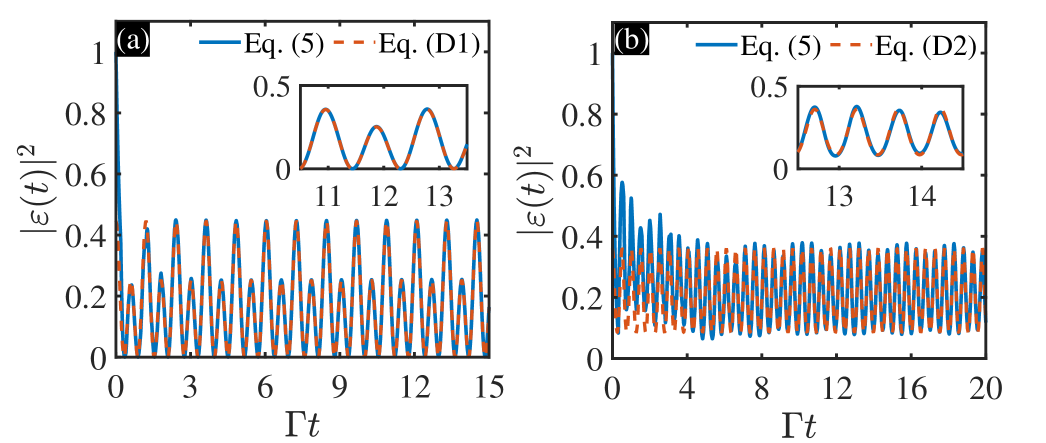
Figure 17: The non-equal amplitude oscillating bound states of a giant atom. The orange-dashed and blue-solid lines correspond to the analytical solutions in Eqs. (42) and (LABEL:D2) and numerical simulation with Eq. (5), respectively. The parameters chosen are (a) $N=5,k_{0}=4,k_{1}=23,k_{2}=25,\omega_{0}\tau_{0}=8\pi,\Gamma\tau_{0}=0.0642\pi$; (b) $N=8,k_{0}=8,k_{1}=71,k_{2}=82,\omega_{0}\tau_{0}=17\pi,\Gamma\tau_{0}=0.0989\pi$. $\omega_{k_{n}}$ in (a) and (b) are determined by Eq. (14b).

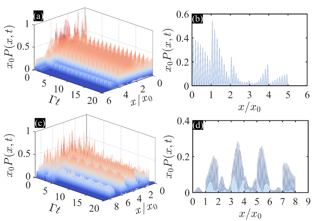
Figure 18: The field intensity $P(x,t)={\left|{\phi(x,t)}\right|^{2}}$ is plotted as a function of $\Gamma t$ and $x/x_{0}$ based on Eq. (6). (a) and (c) show the time evolution of the field intensity $P(x,t)$ in the waveguide correspond to Figs. 17(a) and 17(b), where the parameters $k_{0},k_{1},$ and $k_{2}$ are the same as those in Fig. 17. The colors in (a) and (c) describe the field intensity of the bound states. For clarity, (b) and (d) show the distribution of $P(x,t)$ in the waveguide at $t=20/\Gamma$, which correspond to (a) and (c). The blue-dotted line is the numerical simulation of Eq. (6). The other parameters are the same as those in Fig. 17.

Appendix C Discussion on the coexistence of multiple bound states

When $k_{1}$ and $k_{2}$ are simultaneously the two solutions of Eq. (15a), the parameters $\omega\tau_{0}$ and $\Gamma\tau_{0}$ have to be

$$\omega_{0}\tau_{0}= \frac{2k_{1}\pi}{N}-\frac{2(k_{1}-k_{2})\pi}{N}\frac{\cot\left(\frac{k_{1}\pi}{N}\right)}{\cot\left(\frac{k_{1}\pi}{N}\right)-\cot\left(\frac{k_{2}\pi}{N}\right)}>0,$$ (39)

$$\Gamma\tau_{0}= \frac{4(k_{1}-k_{2})\pi}{N^{2}}\frac{1}{\cot\left(\frac{k_{1}\pi}{N}\right)-\cot\left(\frac{k_{2}\pi}{N}\right)}>0.$$

If both the bound state conditions (12a) and (15a) are satisfied, three bound states coexist in the system. Substituting ${\omega_{0}}{\tau_{0}}={\omega_{{k_{0}}}}{\tau_{0}}=2{k_{0}}\pi$ into Eq. (15a) leads to $\Gamma{\tau_{0}}=\left({\frac{{2{k_{1}}\pi}}{N}-2{k_{0}}\pi}\right)\frac{2}{N}\tan\left({\frac{{{k_{1}}\pi}}{N}}\right)=\frac{{4\pi}}{{{N^{2}}}}\tan\left({\frac{{{k_{1}}\pi}}{N}}\right)\left({{k_{1}}-{k_{0}}N}\right)$, which is reduced to $\Gamma{\tau_{0}}=q\frac{{4\pi}}{{{N^{2}}}}\tan\left({\frac{{q\pi}}{N}}\right)$ by introducing ${k_{1}}=N{k_{0}}+q$, where ${q,~{}~{}{k_{0}},~{}~{}{k_{1}}\in{{\mathbb{N}}_{+}}}$. We get ${k_{2}}=N{k_{0}}-q$ due to the tangent function being an odd function. Collecting all these together, the frequencies in Eq. (22) read

$${\omega_{{k_{0}}}}{\tau_{0}} =2{k_{0}}\pi,$$ (40)

$${\omega_{{k_{1}}}}{\tau_{0}} =\frac{{2{k_{1}}\pi}}{N}=2{k_{0}}\pi+\frac{{2q\pi}}{N},$$

$${\omega_{{k_{2}}}}{\tau_{0}} =\frac{{2{k_{2}}\pi}}{N}=2{k_{0}}\pi-\frac{{2q\pi}}{N}.$$

With the same method, we obtain the frequencies in Eq. (23) when Eqs. (12b) and (15a) exist together

$${\omega_{{k_{0}}}}{\tau_{0}} =(2{k_{0}}+1)\pi,$$ (41)

$${\omega_{{k_{1}}}}{\tau_{0}} =\frac{{2{k_{1}}\pi}}{N}=2{k_{0}}\pi-\frac{{2q\pi}}{N},$$

$${\omega_{{k_{2}}}}{\tau_{0}} =\frac{{2{k_{2}}\pi}}{N}=(2{k_{0}}+1)\pi+\frac{{2q\pi}}{N}.$$

Replacing $N$ with $N+1$, a series of results can be got when Eq. (15b) holds or both Eqs. (12) and (15b) are satisfied.

Appendix D The non-equal amplitude oscillating bound states caused by the coexistence of Eqs. (12) and (15b)

Here, we focus on the coexistence of three mode bound states when Eqs. (12) and (15b) are met simultaneously, which results in that Eqs. (22) and (23) become

$$\varepsilon(t) = \frac{1}{{1+\frac{\Gamma}{2}\sum\limits_{m,n=1}^{N}{\left[{-\left|{m-n}\right|{\tau_{0}}+\left({m+n}\right){\tau_{0}}}\right]}}}{e^{-i2{k_{0}}\pi t/{\tau_{0}}}}$$ (42)

$$+\frac{{2{{\sin}^{2}}({\omega_{{k_{1}}}}{\tau_{0}}/2)}}{{2{{\sin}^{2}}({\omega_{{k_{1}}}}{\tau_{0}}/2)+(N+1)\Gamma{\tau_{0}}}}{e^{-i2{k_{1}}\pi t/\left[{(N+1){\tau_{0}}}\right]}}+\frac{{2{{\sin}^{2}}({\omega_{{k_{2}}}}{\tau_{0}}/2)}}{{2{{\sin}^{2}}({\omega_{{k_{2}}}}{\tau_{0}}/2)+(N+1)\Gamma{\tau_{0}}}}{e^{-i2{k_{2}}\pi t/\left[{(N+1){\tau_{0}}}\right]}},$$

$$\varepsilon(t) = \frac{1}{{1+\frac{\Gamma}{2}\sum\limits_{m,n=1}^{N}{\left[{-\left|{m-n}\right|{\tau_{0}}{{\left({-1}\right)}^{\left|{m-n}\right|}}+\left({m+n}\right){\tau_{0}}{{\left({-1}\right)}^{\left({m+n}\right)}}}\right]}}}{e^{-i(2{k_{0}}+1)\pi t/{\tau_{0}}}}$$

$$+\frac{{2{{\sin}^{2}}({\omega_{{k_{1}}}}{\tau_{0}}/2)}}{{2{{\sin}^{2}}({\omega_{{k_{1}}}}{\tau_{0}}/2)+(N+1)\Gamma{\tau_{0}}}}{e^{-i2{k_{1}}\pi t/\left[{(N+1){\tau_{0}}}\right]}}+\frac{{2{{\sin}^{2}}({\omega_{{k_{2}}}}{\tau_{0}}/2)}}{{2{{\sin}^{2}}({\omega_{{k_{2}}}}{\tau_{0}}/2)+(N+1)\Gamma{\tau_{0}}}}{e^{-i2{k_{2}}\pi t/\left[{(N+1){\tau_{0}}}\right]}}.$$

We take the atomic excitation probability as a function of ${\Gamma t}$ in Fig. 17. The excitation probability of the giant atom is a non-equal amplitude oscillating bound state, which is consistent with the case when both Eqs. (12) and (15a) are met. In Fig. 18, we plot the corresponding time evolution of the field intensity in the waveguide and the field intensity distribution at $t=20/\Gamma$. We note that there is a clear difference in frequency and amplitude between Figs. 17(a) and 17(b), which is similar to the phenomenon between Figs. 9(a) and 9(b), although they are both superpositions of three different bound modes. In order to understand the reason for the difference, we start with the expression of the atomic excitation probability amplitude. When case (iii) in Sec. IV is satisfied, the long-time dynamics of the giant atom can be written as

$$\varepsilon(t)={A_{0}}{e^{-i{\omega_{{k_{0}}}}t/{\tau_{0}}}}+{A_{1}}{e^{-i{\omega_{{k_{1}}}}t/{\tau_{0}}}}+{A_{2}}{e^{-i{\omega_{{k_{2}}}}t/{\tau_{0}}}},$$ (44)

which results in

$${\left|{\varepsilon(t)}\right|^{2}}= {\left|{{A_{0}}}\right|^{2}}+{\left|{{A_{1}}}\right|^{2}}+{\left|{{A_{2}}}\right|^{2}}$$ (45)

$$+2{A_{0}}{A_{1}}\cos\left[{\left({{\omega_{{k_{0}}}}-{\omega_{{k_{1}}}}}\right){\tau_{0}}t}\right]+2{A_{0}}{A_{2}}\cos\left[{\left({{\omega_{{k_{0}}}}-{\omega_{{k_{2}}}}}\right){\tau_{0}}t}\right]+2{A_{1}}{A_{2}}\cos\left[{\left({{\omega_{{k_{1}}}}-{\omega_{{k_{2}}}}}\right){\tau_{0}}t}\right],$$

where

$${A_{0}}=\frac{1}{{1+\frac{\Gamma}{2}\sum\limits_{m,n=1}^{N}{\left[{-\left|{m-n}\right|{\tau_{0}}+\left({m+n}\right){\tau_{0}}}\right]}}},~{}~{}{A_{\alpha}}=\frac{{2{{\sin}^{2}}({\omega_{{k_{\alpha}}}}{\tau_{0}}/2)}}{{2{{\sin}^{2}}({\omega_{{k_{\alpha}}}}{\tau_{0}}/2)+N\Gamma{\tau_{0}}}},$$ (46)

with $\alpha=1,2$. Together with Eq. (40), we get $|{{\omega_{{k_{0}}}}{\tau_{0}}-{\omega_{{k_{1}}}}{\tau_{0}}}|=|{{\omega_{{k_{0}}}}{\tau_{0}}-{\omega_{{k_{2}}}}{\tau_{0}}}|=2q\pi{\tau_{0}}/N,|{{\omega_{{k_{1}}}}{\tau_{0}}-{\omega_{{k_{2}}}}{\tau_{0}}}|=4q\pi{\tau_{0}}/N$, and substituting them into Eq. (46) leads to

$${\left|{\varepsilon(t)}\right|^{2}}= {\left|{{A_{0}}}\right|^{2}}+{\left|{{A_{1}}}\right|^{2}}+{\left|{{A_{2}}}\right|^{2}}+2{A_{0}}\left({{A_{1}}+{A_{2}}}\right)\cos(\Upsilon{\tau_{0}}t)+2{A_{1}}{A_{2}}\cos(2\Upsilon{\tau_{0}}t),$$ (47)

with $\Upsilon=2q\pi/N$. Therefore, the non-equal amplitude oscillating bound state is a superposition of the cosine functions of two persistent oscillations with amplitudes $2{A_{0}}\left({{A_{1}}+{A_{2}}}\right)$ and $2{A_{1}}{A_{2}}$, respectively. We define the difference between the amplitudes of the two cosine functions as ${\Delta_{A}}=\left|{2{A_{0}}\left({{A_{1}}+{A_{2}}}\right)-2{A_{1}}A}\right|$. As shown in Figs. 9(a) and 17(a), the difference between two adjacent peaks is small when ${\Delta_{A}}$ is large. On the contrary, when ${\Delta_{A}}$ becomes small, the difference between two adjacent wave peaks becomes large as depicted in Figs. 17(b) and 9(b). This is the essential reason leading to the difference between Figs. 9(a) and 9(b) (Figs. 17(a) and 17(b)).

References

- (1) A. F. Kockum, A. Miranowicz, S. De Liberato, S. Savasta, and F. Nori, Ultrastrong coupling between light and matter, Nat. Rev. Phys. 1, 19 (2019).
- (2) H. J. Kimble, Strong interactions of single atoms and photons in cavity QED, Phys. Scr. T76, 127 (1998).
- (3) J. M. Raimond, M. Brune, and S. Haroche, Manipulating quantum entanglement with atoms and photons in a cavity, Rev. Mod. Phys. 73, 565 (2001).
- (4) H. Walther, B. T. H. Varcoe, B. G. Englert, and T. Becker, Cavity quantum electrodynamics, Rep. Prog. Phys. 69, 1325 (2006).
- (5) A. Blais, A. L. Grimsmo, S. M. Girvin, and A. Wallraff, Circuit quantum electrodynamics, Rev. Mod. Phys. 93, 025005 (2021).
- (6) A. Blais, R. S. Huang, A. Wallraff, S. M. Girvin, and R. J. Schoelkopf, Cavity quantum electrodynamics for superconducting electrical circuits: An architecture for quantum computation, Phys. Rev. A 69, 062320 (2004).
- (7) A. Wallraff, D. I. Schuster, A. Blais, L. Frunzio, R. S. Huang, J. Majer, S. Kumar, S. M. Girvin, and R. J. Schoelkopf, Strong coupling of a single photon to a superconducting qubit using circuit quantum electrodynamics, Nature (London) 431, 162 (2004).
- (8) D. Roy, C. M. Wilson, and O. Firstenberg, Colloquium: Strongly interacting photons in one-dimensional continuum, Rev. Mod. Phys. 89, 021001 (2017).
- (9) X. Gu, A. F. Kockum, A. Miranowicz, Y. X. Liu, and F. Nori, Microwave photonics with superconducting quantum circuits, Phys. Rep. 718, 1 (2017).
- (10) A. S. Sheremet, M. I. Petrov, I. V. Iorsh, A. V. Poshakinskiy, and A. N. Poddubny, Waveguide quantum electrodynamics: collective radiance and photon-photon correlations, Rev. Mod. Phys. 95, 015002 (2023).
- (11) P. Goy, J. M. Raimond, M. Gross, and S. Haroche, Observation of Cavity-Enhanced Single-Atom Spontaneous Emission, Phys. Rev. Lett. 50, 1903 (1983).
- (12) D. Leibfried, R. Blatt, C. Monroe, and D. Wineland, Quantum dynamics of single trapped ions, Rev. Mod. Phys. 75, 281 (2003).
- (13) R. Miller, T. E. Northup, K. M. Birnbaum, A. Boca, A. D. Boozer, and H. J. Kimble, Trapped atoms in cavity QED: coupling quantized light and matter, J. Phys. B: At. Mol. Opt. Phys. 38, S551 (2005).
- (14) S. Haroche, Nobel Lecture: Controlling photons in a box and exploring the quantum to classical boundary, Rev. Mod. Phys. 85, 1083 (2013).
- (15) D. F. Walls and G. J. Milburn, Quantum Optics, 2nd ed. (Springer, Berlin, 2008).
- (16) R. Manenti, A. F. Kockum, A. Patterson, T. Behrle, J. Rahamim, G. Tancredi, F. Nori, and P. J. Leek, Circuit quantum acoustodynamics with surface acoustic waves, Nat. Commun. 8, 975 (2017).
- (17) J. Q. You and F. Nori, Atomic physics and quantum optics using superconducting circuits, Nature (London) 474, 589 (2011).
- (18) A. F. Kockum and F. Nori, Quantum Bits with Josephson Junctions, in Fundamentals and Frontiers of the Josephson Effect, edited by F. Tafuri (Springer, Berlin, 2019), pp. 703-741.
- (19) P. Krantz, M. Kjaergaard, F. Yan, T. P. Orlando, S. Gustavsson, and W. D. Oliver, A quantum engineer’s guide to superconducting qubits, Appl. Phys. Rev. 6, 021318 (2019).
- (20) M. V. Gustafsson, T. Aref, A. F. Kockum, M. K. Ekström, G. Johansson, and P. Delsing, Propagating phonons coupled to an artificial atom, Science 346, 207 (2014).
- (21) A. Frisk Kockum, in International Symposium on Mathematics, Quantum Theory, and Cryptography, edited by T. Takagi, M. Wakayama, K. Tanaka, N. Kunihiro, K. Kimoto, and Y. Ikematsu (Springer Singapore, Singapore, 2021), pp. 125-146.
- (22) G. Andersson, B. Suri, L. Z. Guo, T. Aref, and P. Delsing, Non-exponential decay of a giant artificial atom, Nat. Phys. 15, 1123 (2019).
- (23) B. Kannan, M. J. Ruckriegel, D. L. Campbell, A. F. Kockum, J. Braumüller, D. K. Kim, M. Kjaergaard, P. Krantz, A. Melville, B. M. Niedzielski, A. Vepsäläinen, R. Winik, J. L. Yoder, F. Nori, T. P. Orlando, S. Gustavsson, and W. D. Oliver, Waveguide quantum electrodynamics with superconducting artificial giant atoms, Nature (London) 583, 775 (2020).
- (24) A. F. Kockum, P. Delsing, and G. Johansson, Designing frequency-dependent relaxation rates and Lamb shifts for a giant artificial atom, Phys. Rev. A 90, 013837 (2014).
- (25) A. M. Vadiraj, A. Ask, T. G. McConkey, I. Nsanzineza, C. W. Sandbo Chang, A. F. Kockum, and C. M. Wilson, Engineering the level structure of a giant artificial atom in waveguide quantum electrodynamics, Phys. Rev. A 103, 023710 (2021).
- (26) A. F. Kockum, G. Johansson, and F. Nori, Decoherence-Free Interaction between Giant Atoms in Waveguide Quantum Electrodynamics, Phys. Rev. Lett. 120, 140404 (2018).
- (27) A. Carollo, D. Cilluffo, and F. Ciccarello, Mechanism of decoherence-free coupling between giant atoms, Phys. Rev. Research 2, 043184 (2020).
- (28) L. Du, L. Z. Guo, and Y. Li, Complex decoherence-free interactions between giant atoms, Phys. Rev. A 107, 023705 (2023).
- (29) A. Soro, C. S. Muñoz, and A. F. Kockum, Interaction between giant atoms in a one-dimensional structured environment, Phys. Rev. A 107, 013710 (2023).
- (30) A. Soro and A. F. Kockum, Chiral quantum optics with giant atoms, Phys. Rev. A 105, 023712 (2022).
- (31) D. Cilluffo, A. Carollo, S. Lorenzo, J. A. Gross, G. M. Palma, and F. Ciccarello, Collisional picture of quantum optics with giant emitters, Phys. Rev. Research 2, 043070 (2020).
- (32) L. Z. Guo, A. Grimsmo, A. F. Kockum, M. Pletyukhov, and G. Johansson, Giant acoustic atom: A single quantum system with a deterministic time delay, Phys. Rev. A 95, 053821 (2017).
- (33) S. Longhi, Photonic simulation of giant atom decay, Opt. Lett. 45, 3017 (2020).
- (34) S. J. Guo, Y. D. Wang, T. Purdy, and J. Taylor, Beyond spontaneous emission: Giant atom bounded in the continuum, Phys. Rev. A 102, 033706 (2020).
- (35) L. Du, Y. T. Chen, Y. Zhang, and Y. Li, Giant atoms with time-dependent couplings, Phys. Rev. Research 4, 023198 (2022).
- (36) L. Z. Guo, A. F. Kockum, F. Marquardt, and G. Johansson, Oscillating bound states for a giant atom, Phys. Rev. Research 2, 043014 (2020).
- (37) K. H. Lim, W. K. Mok, and L. C. Kwek, Oscillating bound states in non-Markovian photonic lattices, Phys. Rev. A 107, 023716 (2023).
- (38) W. Zhao and Z. H. Wang, Single-photon scattering and bound states in an atom-waveguide system with two or multiple coupling points, Phys. Rev. A 101, 053855 (2020).
- (39) X. Wang, T. Liu, A. F. Kockum, H. R. Li, and F. Nori, Tunable Chiral Bound States with Giant Atoms, Phys. Rev. Lett. 126, 043602 (2021).
- (40) H. Xiao, L. J. Wang, Z. H. Li, X. F. Chen, and L. Q. Yuan, Bound state in a giant atom-modulated resonators system, npj Quantum Inf. 8, 80 (2022).
- (41) C. Vega, M. Bello, D. Porras, and A. González-Tudela, Qubit-photon bound states in topological waveguides with long-range hoppings, Phys. Rev. A 104, 053522 (2021).
- (42) X. L. Yin, W. B. Luo, and J. Q. Liao, Non-Markovian disentanglement dynamics in double-giant-atom waveguide-QED systems, Phys. Rev. A 106, 063703 (2022).
- (43) W. J. Cheng, Z. H. Wang, and Y. X. Liu, Topology and retardation effect of a giant atom in a topological waveguide, Phys. Rev. A 106, 033522 (2022).
- (44) A. Ask, Y. L. L. Fang, and A. F. Kockum, Synthesizing electromagnetically induced transparency without a control field in waveguide QED using small and giant atoms, arXiv:2011.15077.
- (45) W. Zhao, Y. Zhang, and Z. H. Wang, Phase-modulated Autler-Townes splitting in a giant-atom system within waveguide QED, Front. Phys. 17, 42506 (2022).
- (46) Y. T. Zhu, S. Xue, R. B. Wu, W. L. Li, Z. H. Peng, and M. Jiang, Spatial-nonlocality-induced non-Markovian electromagnetically induced transparency in a single giant atom, Phys. Rev. A 106, 043710 (2022).
- (47) L. Du, Y. Zhang, J. H. Wu, A. F. Kockum, and Y. Li, Giant Atoms in a Synthetic Frequency Dimension, Phys. Rev. Lett. 128, 223602 (2022).
- (48) X. J. Zhang, W. J. Cheng, Z. R. Gong, T. Y. Zheng, and Z. H. Wang, Superconducting giant atom waveguide QED: Quantum Zeno and Anti-Zeno effects in ultrastrong coupling regime, arXiv:2205.03674.
- (49) D. D. Noachtar, J. Knörzer, and R. H. Jonsson, Nonperturbative treatment of giant atoms using chain transformations, Phys. Rev. A 106, 013702 (2022).
- (50) L. Du, Y. Zhang, and Y. Li, A giant atom with modulated transition frequency, Front. Phys. 18, 12301 (2023).
- (51) X. Wang, Z. M. Gao, J. Q. Li, H. B. Zhu, and H. R. Li, Unconventional quantum electrodynamics with a Hofstadter-ladder waveguide, Phys. Rev. A 106, 043703 (2022).
- (52) S. Terradas-Briansó, C. A. González-Gutiérrez, F. Nori, L. Martín-Moreno, and D. Zueco, Ultrastrong waveguide QED with giant atoms, Phys. Rev. A 106, 063717 (2022).
- (53) A. C. Santos and R. Bachelard, Generation of Maximally Entangled Long-Lived States with Giant Atoms in a Waveguide, Phys. Rev. Lett. 130, 053601 (2023).
- (54) X. P. Yang, Z. K. Han, W. Zheng, D. Lan, and Y. Yu, The interference between a giant atom and an internal resonator, Commun. Theor. Phys. 73, 115104 (2021).
- (55) Q. Y. Qiu, Y. Wu, and X. Y. Lü, Collective radiance of giant atoms in non-Markovian regime, Sci. China Phys. Mech. Astron. 66, 224212 (2023).
- (56) X. Wang and H. R. Li, Chiral quantum network with giant atoms, Quantum Sci. Technol. 7, 035007 (2022).
- (57) Z. Q. Wang, Y. P. Wang, J. G. Yao, R. C. Shen, W. J. Wu, J. Qian, J. Li, S. Y. Zhu, and J. Q. You, Giant spin ensembles in waveguide magnonics, Nat. Commun. 13, 7580 (2022).
- (58) J. Y. Liu, J. W. Jin, H. Y. Liu, Y. Ming, and R. C. Yang, Optical multi-Fano-like phenomena with giant atom-waveguide systems, Quantum Inf. Process 22, 74 (2023).
- (59) E. Sánchez-Burillo, D. Porras, and A. González-Tudela, Limits of photon-mediated interactions in one-dimensional photonic baths, Phys. Rev. A 102, 013709 (2020).
- (60) X. J. Zhang, C. G. Liu, Z. R. Gong, and Z. H. Wang, Quantum interference and controllable magic cavity QED via a giant atom in coupled resonator waveguide, Phys. Rev. A 108, 013704 (2023).
- (61) X. Y. Li, W. Zhao, and Z. H. Wang, Controlling photons by phonons via giant atom in a waveguide QED setup, Opt. Lett. 48, 3595 (2023).
- (62) Y. T. Chen, L. Du, Y. Zhang, L. Z. Guo, J. H. Wu, M. Artoni, and G. C. La Rocca, Giant-Atom Effects on Population and Entanglement Dynamics of Rydberg Atoms, arXiv:2304.14713.
- (63) X. Wang, H. B. Zhu, T. Liu, and F. Nori, Realizing quantum optics in structured environments with giant atoms, arXiv:2304.10710.
- (64) L. Du, Y. T. Chen, Y. Zhang, Y. Li, and J. H. Wu, Decay dynamics of a giant atom in a structured bath with broken time-reversal symmetry, Quantum Sci. Technol. 8, 045010 (2023).
- (65) P. C. Kuo, J. D. Lin, Y. C. Huang, and Y. N. Chen, Controlling periodic Fano resonances of quantum acoustic waves with a giant atom coupled to microwave waveguide, arXiv:2307.07949.
- (66) W. Z. Jia and M. T. Yu, Atom-photon dressed states in a waveguide-QED system with multiple giant atoms coupled to a resonator-array waveguide, arXiv:2304.02072.
- (67) X. L. Yin and J. Q. Liao, Giant-atom entanglement in waveguide-QED systems including non-Markovian effect, arXiv:2303.14746.
- (68) J. Y. Liu, J. W. Jin, X. M. Zhang, Z. G. Zheng, H. Y. Liu, Y. Ming, and R. C. Yang, Distant entanglement generation and controllable information transfer via magnon-waveguide systems, Results in Physics 52, 106854 (2023).
- (69) L. Du, Z. H. Wang, and Y. Li, Controllable optical response and tunable sensing based on self interference in waveguide QED systems, Opt. Express 29, 3038 (2021).
- (70) C. Wang, X. S. Ma, and M. T. Cheng, Giant atom-mediated single photon routing between two waveguides, Opt. Express 29, 40116 (2021).
- (71) Y. Q. Zhang, Z. H. Zhu, K. K. Chen, Z. H. Peng, W. J. Yin, Y. Yang, Y. Q. Zhao, Z. Y. Lu, Y. F. Chai, Z. Z. Xiong, and L. Tan, Controllable single-photon routing between two waveguides by two giant two-level atoms, Front. Phys. 10, 1054299 (2022).
- (72) Y. Q. Zhang, Z. H. Zhu, Z. H. Peng, Z. H. Peng, W. J. Yin, Y. Yang, Y. Q. Zhao, Z. Y. Lu, Y. F. Chai, Z. Z. Xiong, and L. Tan, Tunable single-photon routing between two single-mode waveguides by a giant -type three-level atom, Optik 274, 170568 (2023).
- (73) L. Du and Y. Li, Single-photon frequency conversion via a giant -type atom, Phys. Rev. A 104, 023712 (2021).
- (74) W. J. Gu, H. Huang, Z. Yi, L. Chen, L. H. Sun, and H. T. Tan, Correlated two-photon scattering in a 1D waveguide coupled to two- or three-level giant atoms, arXiv:2306.13836.
- (75) W. J. Cheng, Z. H. Wang, and T. Tian, The single- and two-photon scattering in the waveguide QED coupling to a giant atom, Laser Phys. 33, 085203 (2023).
- (76) Q. Y. Cai and W. Z. Jia, Coherent single-photon scattering spectra for a giant-atom waveguide-QED system beyond the dipole approximation, Phys. Rev. A 104, 033710 (2021).
- (77) S. L. Feng and W. Z. Jia, Manipulating single-photon transport in a waveguide-QED structure containing two giant atoms, Phys. Rev. A 104, 063712 (2021).
- (78) J. P. Zou, R. Y. Gong, and Z. L. Xiang, Tunable Single-Photon Scattering of a Giant -type Atom in a SQUID-Chain Waveguide, Front. Phys. 10, 896827 (2022).
- (79) X. L. Yin, Y. H. Liu, J. F. Huang, and J. Q. Liao, Single-photon scattering in a giant-molecule waveguide-QED system, Phys. Rev. A 106, 013715 (2022).
- (80) H. W. Yu, Z. H. Wang, and J. H. Wu, Entanglement preparation and nonreciprocal excitation evolution in giant atoms by controllable dissipation and coupling, Phys. Rev. A 104, 013720 (2021).
- (81) J. Zhou, X. L. Yin, and J. Q. Liao, Chiral and nonreciprocal single-photon scattering in a chiral-giant-molecule waveguide-QED system, Phys. Rev. A 107, 063703 (2023).
- (82) L. Du, M. R. Cai, J. H. Wu, Z. H. Wang, and Y. Li, Single-photon nonreciprocal excitation transfer with non-Markovian retarded effects, Phys. Rev. A 103, 053701 (2021).
- (83) J. J. Wang, F. D. Li, and X. X. Yi, Giant atom induced zero modes and localization in the nonreciprocal Su-Schrieffer-Heeger chain, arXiv:2211.01819.
- (84) L. Du, Y. T. Chen, and Y. Li, Nonreciprocal frequency conversion with chiral -type atoms, Phys. Rev. Research 3, 043226 (2021).
- (85) Y. T. Chen, L. Du, L. Z. Guo, Z. H. Wang, Y. Zhang, Y. Li, and J. H. Wu, Nonreciprocal and chiral single-photon scattering for giant atoms, Commun. Phys. 5, 215 (2022).
- (86) N. Liu, X. Wang, X. Wang, X. S. Ma, and M. T. Cheng, Tunable single photon nonreciprocal scattering based on giant atom-waveguide chiral couplings, Opt. Express 30, 23428 (2022).
- (87) X. J. Sun, W. X. Liu, H. Chen, and H. R. Li, Tunable single-photon nonreciprocal scattering and targeted router in a giant atom-waveguide system with chiral couplings, Commun. Theor. Phys. 75, 035103 (2023).
- (88) A. González-Tudela, C. S. Muñoz, and J. I. Cirac, Engineering and Harnessing Giant Atoms in High-Dimensional Baths: A Proposal for Implementation with Cold Atoms, Phys. Rev. Lett. 122, 203603 (2019).
- (89) J. Eschner, C. Raab, F. Schmidt-Kaler, and R. Blatt, Light interference from single atoms and their mirror images, Nature (London) 413, 495 (2001).
- (90) T. Tufarelli, M. S. Kim, and F. Ciccarello, Non-Markovianity of a quantum emitter in front of a mirror, Phys. Rev. A 90, 012113 (2014).
- (91) P. O. Guimond, M. Pletyukhov, H. Pichler, and P. Zoller, Delayed coherent quantum feedback from a scattering theory and a matrix product state perspective, Quantum Sci. Technol. 2, 044012 (2017).
- (92) G. Calajó, Y. L. L. Fang, H. U. Baranger, and F. Ciccarello, Exciting a Bound State in the Continuum through Multiphoton Scattering Plus Delayed Quantum Feedback, Phys. Rev. Lett. 122, 073601 (2019).
- (93) P. W. Milonni and P. L. Knight, Retardation in the resonant interaction of two identical atoms, Phys. Rev. A 10, 1096 (1974).
- (94) H. X. Zheng and H. U. Baranger, Persistent Quantum Beats and Long-Distance Entanglement from Waveguide-Mediated Interactions, Phys. Rev. Lett. 110, 113601 (2013).
- (95) C. Gonzalez-Ballestero, F. J. García-Vidal, and E. Moreno, Non-Markovian effects in waveguide-mediated entanglement, New J. Phys. 15, 073015 (2013).
- (96) M. Laakso and M. Pletyukhov, Scattering of Two Photons from Two Distant Qubits: Exact Solution, Phys. Rev. Lett. 113, 183601 (2014).
- (97) C. Gonzalez-Ballestero, E. Moreno, and F. J. García-Vidal, Generation, manipulation, and detection of two-qubit entanglement in waveguide QED, Phys. Rev. A 89, 042328 (2014).
- (98) Y. L. L. Fang and H. U. Baranger, Waveguide QED: Power spectra and correlations of two photons scattered off multiple distant qubits and a mirror, Phys. Rev. A 91, 053845 (2015).
- (99) P. O. Guimond, A. Roulet, H. N. Le, and V. Scarani, Rabi oscillation in a quantum cavity: Markovian and non-Markovian dynamics, Phys. Rev. A 93, 023808 (2016).
- (100) T. Ramos, B. Vermersch, P. Hauke, H. Pichler, and P. Zoller, Non-Markovian dynamics in chiral quantum networks with spins and photons, Phys. Rev. A 93, 062104 (2016).
- (101) T. Tufarelli, F. Ciccarello, and M. S. Kim, Dynamics of spontaneous emission in a single-end photonic waveguide, Phys. Rev. A 87, 013820 (2013).
- (102) F. Dinc, İ. Ercan, and A. M. Brańczyk, Exact Markovian and non-Markovian time dynamics in waveguide QED: collective interactions, bound states in continuum, superradiance and subradiance, Quantum 3, 213 (2019).
- (103) A. Ask, M. Ekström, P. Delsing, and G. Johansson, Cavity-free vacuum-Rabi splitting in circuit quantum acoustodynamics, Phys. Rev. A 99, 013840 (2019).
- (104) J. Claudon, J. Bleuse, N. S. Malik, M. Bazin, P. Jaffrennou, N. Gregersen, C. Sauvan, P. Lalanne, and J. M. Gérard, A highly efficient single-photon source based on a quantum dot in a photonic nanowire, Nat. Photonics 4, 174 (2010).
- (105) J. Bleuse, J. Claudon, M. Creasey, N. S. Malik, J. M. Gérard, I. Maksymov, J. P. Hugonin, and P. Lalanne, Inhibition, Enhancement, and Control of Spontaneous Emission in Photonic Nanowires, Phys. Rev. Lett. 106, 103601 (2011).
- (106) M. E. Reimer, G. Bulgarini, N. Akopian, M. Hocevar, M. B. Bavinck, M. A. Verheijen, E. P. A. M. Bakkers, L. P. Kouwenhoven, and V. Zwiller, Bright single-photon sources in bottom-up tailored nanowires, Nat. Commun. 3, 737 (2012).
- (107) G. Bulgarini, M. E. Reimer, T. Zehender, M. Hocevar, E. P. A. M. Bakkers, L. P. Kouwenhoven, and V. Zwiller, Spontaneous emission control of single quantum dots in bottom-up nanowire waveguides, Appl. Phys. Lett. 100, 121106 (2012).
- (108) M. Bradford and J. T. Shen, Spontaneous emission in cavity QED with a terminated waveguide, Phys. Rev. A 87, 063830 (2013).
- (109) C. Y. Chang, L. Lanco, and D. S. Citrin, Quantum stabilization of microcavity excitation in a coupled microcavity-half-cavity system, Phys. Rev. B 101, 024305 (2020).
- (110) K. Sinha, P. Meystre, E. A. Goldschmidt, F. K. Fatemi, S. L. Rolston, and P. Solano, Non-Markovian Collective Emission from Macroscopically Separated Emitters, Phys. Rev. Lett. 124, 043603 (2020).
- (111) Y. L. L. Fang, F. Ciccarello, and H. U. Baranger, Non-Markovian dynamics of a qubit due to single-photon scattering in a waveguide, New J. Phys. 20, 043035 (2018).
- (112) J. Zeng, Y. J. Song, J. Lu, and L. Zhou, Non-Markovianity of an atom in a semi-infinite rectangular waveguide, Chinese Phys. B 32, 030305 (2023).
- (113) K. Barkemeyer, A. Knorr, and A. Carmele, Heisenberg treatment of multiphoton pulses in waveguide QED with time-delayed feedback, Phys. Rev. A 106, 023708 (2022).
- (114) G. Crowder, L. Ramunno, and S. Hughes, Quantum trajectory theory and simulations of nonlinear spectra and multiphoton effects in waveguide-QED systems with a time-delayed coherent feedback, Phys. Rev. A 106, 013714 (2022).
- (115) L. Xin, S. Xu, X. X. Yi, and H. Z. Shen, Tunable non-Markovian dynamics with a three-level atom mediated by the classical laser in a semi-infinite photonic waveguide, Phys. Rev. A 105, 053706 (2022).
- (116) K. Barkemeyer, A. Knorr, and A. Carmele, Strongly entangled system-reservoir dynamics with multiphoton pulses beyond the two-excitation limit: Exciting the atom-photon bound state, Phys. Rev. A 103, 033704 (2021).
- (117) J. Kabuss, F. Katsch, A. Knorr, and A. Carmele, Unraveling coherent quantum feedback for Pyragas control, J. Opt. Soc. Am. B 33, C10 (2016).
- (118) H. J. Ding, G. F. Zhang, M. T. Cheng, and G. Q. Cai, Quantum feedback control of a two-atom network closed by a semi-infinite waveguide, arXiv:2306.06373.
- (119) H. J. Ding, N. H. Amini, G. F. Zhang, and J. E. Gough, Quantum coherent and measurement feedback control based on atoms coupled with a semi-infinite waveguide, arXiv:2307.16876.
- (120) J. Wang, Y. N. Wu, and S. X. Song, Witnessing Quantum Speedup through Mutual Information, Ann. Phys. (Berlin) 531, 1900225 (2019).
- (121) J. Wang, Y. N. Wu, W. Y. Ji, Controlling Speedup Induced by a Hierarchical Environment, Journal of Modern Physics 10, 1177 (2019).
- (122) K. Barkemeyer, R. Finsterhölzl, A. Knorr, and A. Carmele, Revisiting Quantum Feedback Control: Disentangling the Feedback-Induced Phase from the Corresponding Amplitude, Adv. Quantum Technol. 3, 1900078 (2020).
- (123) H. X. Song, X. Q. Sun, J. Lu, and L. Zhou, Spatial Dependent Spontaneous Emission of an Atom in a Semi-Infinite Waveguide of Rectangular Cross Section, Commun. Theor. Phys. 69, 59 (2018).
- (124) P. Lodahl, A. F. van Driel, I. S. Nikolaev, A. Irman, K. Overgaag, D. Vanmaekelbergh, and W. L. Vos, Controlling the dynamics of spontaneous emission from quantum dots by photonic crystals, Nature (London) 430, 654 (2004).
- (125) J. Wang, Y. N. Wu, N. Guo, Z. Y. Xing, Y. Qin, and P. Wang, Classical-driving-assisted entanglement trapping in photonic-crystal waveguides, Opt. Commun. 420, 183 (2018).
- (126) J. Wang, Y. N. Wu, and Z. Y. Xie, Role of flow of information in the speedup of quantum evolution, Sci. Rep. 8, 16870 (2018).
- (127) B. Peropadre, G. Romero, G. Johansson, C. M. Wilson, E. Solano, and J. J. García-Ripoll, Approaching perfect microwave photodetection in circuit QED, Phys. Rev. A 84, 063834 (2011).
- (128) W. K. Mok, J. B. You, L. C. Kwek, and D. Aghamalyan, Microresonators enhancing long-distance dynamical entanglement generation in chiral quantum networks, Phys. Rev. A 101, 053861 (2020).
- (129) N. Roch, M. E. Schwartz, F. Motzoi, C. Macklin, R. Vijay, A. W. Eddins, A. N. Korotkov, K. B. Whaley, M. Sarovar, and I. Siddiqi, Observation of Measurement-Induced Entanglement and Quantum Trajectories of Remote Superconducting Qubits, Phys. Rev. Lett. 112, 170501 (2014).
- (130) C. Eichler, D. Bozyigit, and A. Wallraff, Characterizing quantum microwave radiation and its entanglement with superconducting qubits using linear detectors, Phys. Rev. A 86, 032106 (2012).
- (131) J. T. Shen and S. H. Fan, Theory of single-photon transport in a single-mode waveguide. I. Coupling to a cavity containing a two-level atom, Phys. Rev. A 79, 023837 (2009).
- (132) J. T. Shen and S. H. Fan, Theory of single-photon transport in a single-mode waveguide. II. Coupling to a whispering-gallery resonator containing a two-level atom, Phys. Rev. A 79, 023838 (2009).
- (133) J. T. Shen and S. H. Fan, Coherent Single Photon Transport in a One-Dimensional Waveguide Coupled with Superconducting Quantum Bits, Phys. Rev. Lett. 95, 213001 (2005).
- (134) J. T. Shen and S. H. Fan, Coherent photon transport from spontaneous emission in one-dimensional waveguides, Opt. Lett. 30, 2001 (2005).
- (135) B. Zhang, S. J. You, and M. Lu, Enhancement of spontaneous entanglement generation via coherent quantum feedback, Phys. Rev. A 101, 032335 (2020).
- (136) Z. Y. Liao, X. D. Zeng, H. Nha, and M. S. Zubairy, Photon transport in a one-dimensional nanophotonic waveguide QED system, Phys. Scr. 91, 063004 (2016).
- (137) A. Chenu, M. Beau, J. Cao, and A. del Campo, Quantum Simulation of Generic Many-Body Open System Dynamics Using Classical Noise, Phys. Rev. Lett. 118, 140403 (2017).
- (138) C. Khripkov and A. Vardi, Quantum Zeno control of coherent dissociation, Phys. Rev. A 84, 021606(R) (2011).
- (139) H. Fröhlich, Interaction of electrons with lattice vibrations, Proc. R. Soc. London A 215, 291 (1952); Q. Ai, Y. Li, H. Zheng, and C. P. Sun, Quantum anti-Zeno effect without rotating wave approximation, Phys. Rev. A 81, 042116 (2010); H. Zheng, Dynamics of a two-level system coupled to Ohmic bath: a perturbation approach, Eur. Phys. J. B 38, 559 (2004).
- (140) Z. G. Lü and H. Zheng, Quantum dynamics of the dissipative two-state system coupled with a sub-Ohmic bath, Phys. Rev. B 75, 054302 (2007).
- (141) T. Shi, Y. Chang, and J. J. García-Ripoll, Ultrastrong Coupling Few-Photon Scattering Theory, Phys. Rev. Lett. 120, 153602 (2018).
- (142) L. Lo and C. K. Law, Quantum radiation from a shaken two-level atom in vacuum, Phys. Rev. A 98, 063807 (2018).
- (143) H. Z. Shen, Q. Wang, and X. X. Yi, Dispersive readout with non-Markovian environments, Phys. Rev. A 105, 023707 (2022); H. Z. Shen, D. X. Li, S. L. Su, Y. H. Zhou, and X. X. Yi, Exact non-Markovian dynamics of qubits coupled to two interacting environments, Phys. Rev. A 96, 033805 (2017); H. Z. Shen, S. L. Su, Y. H. Zhou, and X. X. Yi, Non-Markovian quantum Brownian motion in one dimension in electric fields, Phys. Rev. A 97, 042121 (2018).
- (144) H. Z. Shen, C. Shang, Y. H. Zhou, and X. X. Yi, Unconventional single-photon blockade in non-Markovian systems, Phys. Rev. A 98, 023856 (2018); H. Z. Shen, Q. Wang, J. Wang, and X. X. Yi, Nonreciprocal unconventional photon blockade in a driven dissipative cavity with parametric amplification, Phys. Rev. A 101, 013826 (2020).
- (145) Q. T. Xie, S. Cui, J. P. Cao, L. Amico, and H. Fan, Anisotropic Rabi model, Phys. Rev. X 4, 021046 (2014).
- (146) X. Y. Chen, L. W. Duan, D. Braak, and Q. H. Chen, Multiple ground-state instabilities in the anisotropic quantum Rabi model, Phys. Rev. A 103, 043708 (2021).
- (147) M. A. Rodríguez, P. Tempesta, and P. Winternitz, Reduction of superintegrable systems: The anisotropic harmonic oscillator, Phys. Rev. E 78, 046608 (2008).
- (148) S. Nakajima, Perturbation theory in statistical mechanics, Adv. Phys. 4, 363 (1955).
- (149) H. Fröhlich, Theory of the Superconducting State. I. The Ground State at the Absolute Zero of Temperature, Phys. Rev. 79, 845 (1950).