On Reducing the Execution Latency of Superconducting Quantum Processors via Quantum Program Scheduling

Abstract.

Quantum computing has gained considerable attention, especially after the arrival of the Noisy Intermediate-Scale Quantum (NISQ) era. Quantum processors and cloud services have been made world-wide increasingly available. Unfortunately, programs on existing quantum processors are often executed in series, and the workload could be heavy to the processor. Typically, one has to wait for hours or even longer to obtain the result of a single quantum program on public quantum cloud due to long queue time. In fact, as the scale grows, the qubit utilization rate of the serial execution mode will further diminish, causing the waste of quantum resources. In this paper, to our best knowledge for the first time, the Quantum Program Scheduling Problem (QPSP) is formulated and introduced to improve the utility efficiency of quantum resources. Specifically, a quantum program scheduling method concerning the circuit width, number of measurement shots, and submission time of quantum programs is proposed to reduce the execution latency. We conduct extensive experiments on a simulated Qiskit noise model, as well as on the Xiaohong (from QuantumCTek) superconducting quantum processor. Numerical results show the effectiveness in both QPU time and turnaround time.

1. Introduction

In recent decades, considerable progress has been made in quantum computing (QC). Shor’s algorithm (Shor, 1994) achieves exponential acceleration for factor decomposition, and Grover’s algorithm (Grover, 1996) provides quadratic speedup for unstructured search over classical counterparts. Recently, the development of quantum computers and methods has led us into the so-called Noisy Intermediate-Scale Quantum (NISQ) era (Preskill, 2018), with some evidence on the so-called quantum supremacy, e.g. Google’s superconducting quantum processor Sycamore (Arute et al., 2019). The potential advantage of QC over classical computing are attracting increasing attention.

More and more players like IBM have provided the public access to their quantum computers. This facilitates the validation of quantum algorithms on NISQ devices over the Internet. For example, we have free access to the 7-qubit IBM Perth (Computing, 2019). However, running quantum programs on current quantum computers is non-trivial due to the noise and sparse connectivity of physical qubits. On a NISQ device, the physical qubits are not fully connected. The deployment of two-qubit gates is restricted to pairs of connected qubits. Hence, when mapping logical qubits to their physical counterparts, certain two-qubit gates may be positioned on physically disconnected qubits, rendering them inexecutable. Conventionally, SWAP gates are inserted to change the qubit mapping so that every two-qubit gate can be physically executed.

A more awkward obstacle hindering people from using quantum computers is the unbearably long queue time. Though there exist some quantum cloud services, the growing need for quantum hardware outpaces the open access to quantum hardware. We submit many jobs to IBM Perth. The average number of pending jobs is about 2,540, and the average queue time is about 6.7 hours. The latency of circuit execution is unacceptable, especially when we run Variational Quantum Algorithms (VQAs) (Cerezo et al., 2021), in which plenty of circuits are executed in a single episode to update the parameters. The main reason for this latency is that the submitted quantum programs are executed in series. In other words, only one program is executed on the quantum processor in each execution. Besides, the qubit utilization rate is low. Since entangling a large number of qubits on NISQ devices is challenging due to the noise (Cao et al., 2023), most circuits remain small in width to ensure high fidelity. With the increasing number of physical qubits on QPUs and decreasing error rate, we may execute multiple programs in parallel in each execution, i.e. multi-programming, at a negligible cost of fidelity to reduce the latency. As a result, more people can access quantum resources to facilitate QC.

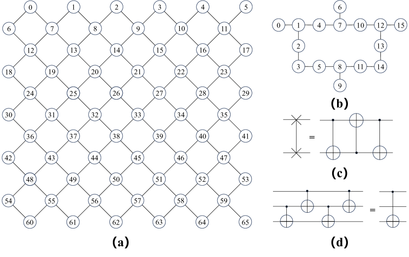
Figure 1. (a) Coupling graph of Xiaohong quantum processor (from QuantumCTek as used in this paper for experiments). (b) Coupling graph of IBM Guadalupe. (c) SWAP gate. (d) BRIDGE gate. SWAP and BRIDGE gates can solve the connectivity constraints on coupling graphs.

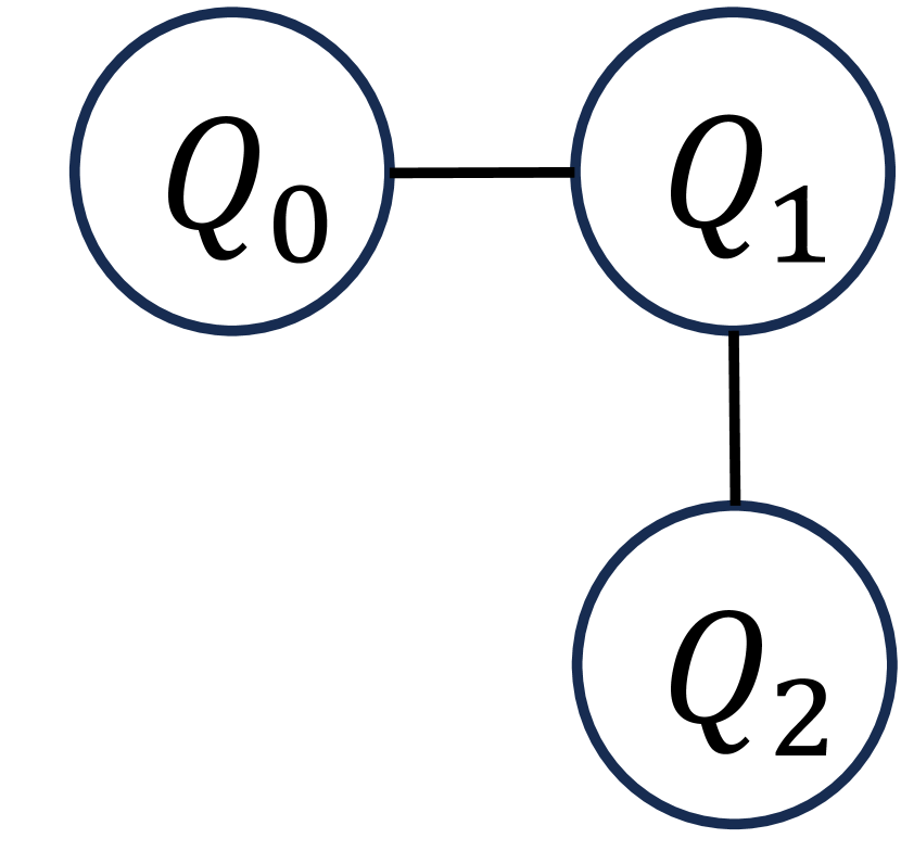
(a)

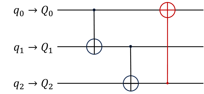
(b)

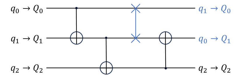
(c)

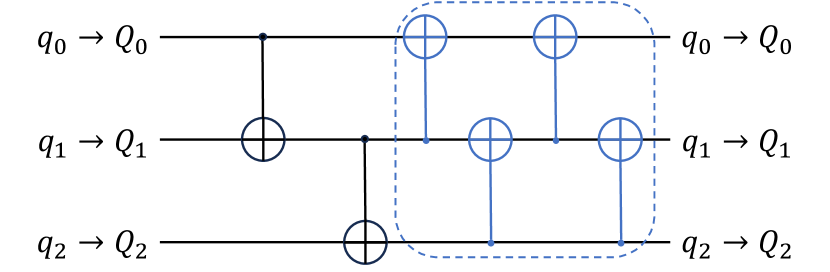
(d)

Figure 2. An example of qubit mapping. (a) Subgraph derived by qubit partitioning. (b) Quantum circuit to be mapped. (The CNOT gate in red cannot be applied, because $Q_{0}$ and $Q_{2}$ are not connected.) (c) Mapped circuit through SWAP gates. (d) Mapped circuit through BRIDGE gates. The SWAP gate changes the mapping in (c) (marked in blue).

However, multi-programming on quantum processors is a complicated task. The execution order of programs will affect the performance of multi-programming. Different from classical process scheduling, we need to consider fidelity apart from time metrics. The QPU should be partitioned in a fair manner to reduce fidelity drop. Unfortunately, fidelity and time metrics often conflict with each other. In this paper, we introduce the Quantum Program Scheduling Problem, which has great practical value in the NISQ era. A novel scheduling method is proposed to tackle this problem. With our priority score and noise-aware initial mapping, our method surpasses baselines in time metrics, and guarantees the fairness and fidelity. The contributions of this paper are:

1) We formulate the Quantum Program Scheduling Problem of reducing the latency of superconducting quantum processors.

2) We propose a novel scheduling method to balance different metrics. Also, three greedy baselines are provided for comparison.

3) Experiments on both the noise model and quantum computer show that our approach significantly reduces the QPU time and turnaround time at a low cost of fidelity.

2. Preliminaries and Related Works

We discuss some basic concepts and loosely related works to ours. To our best knowledge, there still does not exist peer methods for the scheduling problem addressed in our paper.

Quantum Computing. The basic unit in QC is a qubit, which is in superposition of basis states $\ket{0}$ and $\ket{1}$: $\ket{\psi}=a\ket{0}+b\ket{1}$. Likewise, a quantum system with $n$ qubits is in superposition of $2^{n}$ basis states. The evolution of quantum states can be used to generate solutions to specific problems, perhaps in a much faster manner than classical methods. We refer readers to (Nielsen and Chuang, 2010) for detailed backgrounds. Similar to classical circuits, quantum circuits are employed to implement quantum computation of quantum states. Each quantum circuit consists of quantum gates like X gates, RZ gates, CNOT gates, etc. To obtain the result, we have to repeat executing the circuits many times (shots), because quantum measurements will cause the collapse of a superposition state to a basis state. In this paper, we denote the quantum circuits used to solve specific problems as quantum programs.

Quantum Processors. The core of a quantum computer is the quantum processor, aka QPU, which serves to execute quantum circuits. We focus on superconducting quantum processors in this paper. The major properties of a QPU are its basis gates, coupling graph and noise condition. Basis gates are the quantum gates supported on the QPU. All the gates in a quantum program must be converted to basis gates before execution during compiling. As shown in Fig. 1, the coupling graph restricts the connectivity of qubits. Two-qubit gates can only be deployed on connected qubits. Besides, the noise of QPUs in the NISQ era results in gate errors, readout errors, and decoherence, which will corrupt the quantum state and reduce the fidelity. These errors change over time, so they must be calibrated regularly. Nowadays, many quantum processors are open to public through quantum cloud services. Our submitted quantum programs will queue up to be executed. In this paper, we conduct experiments on the Qiskit (Aleksandrowicz et al., 2019) noise model of 16-qubit IBM Guadalupe (Fig. 1b), and 66-qubit Xiaohong (Fig. 1a) quantum processor from the QuantumCTek Quantum Cloud Platform (Platform, 2022).

Qubit Mapping. When logical qubits of a quantum program are mapped to physical qubits on a QPU, the original two-qubit gates may violate the connectivity constraints as shown in Fig. 2(b). A traditional way to solve this problem is to insert SWAP gates. A SWAP gate is implemented by three CNOT gates (Fig. 1c), incurring extra noise. Hence, the number of them is expected to be minimized. Siraichi et al. formally introduce the aforementioned qubit allocation (mapping) problem (Siraichi et al., 2018), which is proved to be NP-complete. Li et al. propose a bidirectional heuristic search (SABRE) to tackle this problem. When inserting a SWAP gate, they consider its impact on two-qubit gates in both the front layer and extended set, significantly reducing the SWAP overhead (Li et al., 2019). Niu et al. take the error rate and execution time of CNOT gates into consideration, and provide BRIDGE gates as an alternative to SWAP gates (Niu et al., 2020). The BRIDGE gate (Fig. 1d) is composed of four CNOT gates, but its effect equals a single CNOT gate. Niu et al. further ameliorate the mapping method by involving the cost of inserted SWAP gates and BRIDGE gates themselves (Niu and Todri-Sanial, 2023).

Quantum Multi-Programming. Quantum multi-programming means running multiple quantum programs simultaneously on a QPU. Das et al. propose the concept of multi-programming NISQ devices to improve throughput. They allocate less noisy physical qubits to logical qubits with higher utility. Qucloud (Liu and Dou, 2021) leverages FN community detection algorithm (Newman, 2004) to partition QPUs, and designs an EPST score to estimate the fidelity of allocation. Resch et al. run multiple QAOA (Farhi et al., 2014) circuits in parallel to accelerate the training process (Resch et al., 2021). Niu et al. reorder the quantum programs according to their CNOT density, and partition QPUs based on the connectivity and error rates of physical qubits (Niu and Todri-Sanial, 2023). These existing methods either neglect the impact of execution order or just focus on multi-programming in single execution.

3. Methodology

In this section, we formally introduce the Quantum Program Scheduling Problem (QPSP) to excavate the importance of the execution order when multi-programming massive quantum programs in the queue of quantum cloud services. Also, a scheduling method and three greedy baselines are proposed to tackle this problem.

3.1. The Quantum Program Scheduling Problem

3.1.1. Definition

Suppose the current job queue $\mathcal{Q}$ is comprised of $K$ quantum jobs to be executed, i.e. $\mathcal{Q}=\{\mathcal{J}_{1},\mathcal{J}_{1},\cdots,\mathcal{J}_{K}\}$. Each job $\mathcal{J}_{i}$ can be represented as a tuple $(p_{i},s_{i},t_{i})$, where $p_{i}$, $s_{i}$, and $t_{i}$ denote the quantum program, number of measurement shots, and submission time, respectively. Then, new jobs $\mathcal{J}_{K+1},\mathcal{J}_{K+2},\cdots$ will be submitted at time $t_{K+1},t_{K+2},\cdots$. For a quantum computer, besides the execution time $t_{e}$ of circuits on the QPU, other procedures like circuit verification, generation of control signals, and communication will cost extra time $t_{m}$ between execution.

Given the coupling graph $\mathcal{G}$, noise calibration data $\mathcal{N}$, and basis gate set $\mathcal{B}$ of the QPU, we need to execute all the jobs submitted during a time period on the QPU. The objective of QPSP is to minimize the execution latency of jobs, and maintain high fidelity.

3.1.2. Metrics

The performance assessment of QPSP is divided into two parts: time and fidelity. Also, fairness should be considered.

Time. For users, they mainly care about the time cost from submission to completion of their quantum job, which we name turnaround time. For suppliers, they may put emphasis on the QPU time of their quantum processors, i.e. circuit running time on QPU. Besides, Trial Reduction Factor (TRF) (Das et al., 2019), which is the ratio of the number of trials when programs run in series to that when programs run in parallel, is included as a time metric in our paper.

Fidelity. The real fidelity of a quantum state is hard to obtain on a quantum computer. By convention, we use the Probability of Successful Trial (PST) (Tannu and Qureshi, 2019), which is defined as the percentage of trials producing the correct result, as our fidelity metric.

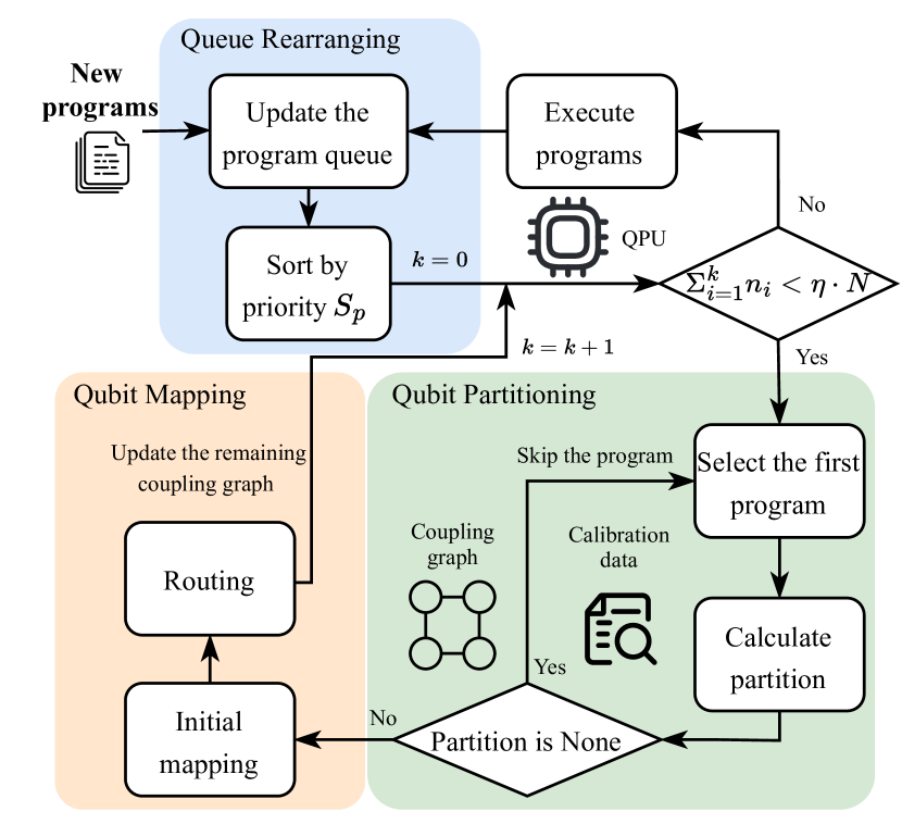
Figure 3. Overview of our method for scheduling.

3.2. Proposed Method

Our proposed method is composed of three parts: queue rearranging, qubit partitioning, and qubit mapping. Fig. 3 shows the overview of our method. In each iteration, we sort the current updated queue by our priority score $S_{p}$. Then, we evaluate quantum programs in the sorted queue one by one, selecting and mapping those programs that can find a partition on the remaining coupling graph, until the number of used physical qubits exceed the limit, i.e. $\Sigma_{i=1}^{k}n_{i}\leq\eta\cdot N$, where $n_{i}$ is the number of qubits (i.e. width) of the $i$-th selected programs, and $k$ is the number of selected programs. $N$ denotes the number of physical qubits, and $\eta\in(0,1]$ is the allowed maximum usage of physical qubits, which influences the average fidelity because higher usage will incur more noise. Then, the mapped programs will be executed in parallel on the QPU. The number of shots is set as the maximum shot number among the mapped programs to ensure all the shot requirements are satisfied, because those programs whose shot requirements are unsatisfied will lead to extra execution overhead in following iterations. The mapped programs are executed in an As Late As Possible (ALAP) manner so that programs with different depth can be completed at the same time to avoid decoherence.

3.2.1. Queue Rearranging

In each iteration, the program queue will be updated due to new submitted programs and executed programs. Akin to the importance of process scheduling for CPUs, the execution order of quantum programs also counts in QPSP. Therefore, we sort quantum programs in the updated queue in ascending order of their priority score. Three properties of a quantum job $\mathcal{J}_{i}$ are considered for its priority score $S_{p}^{(i)}$: the number of qubits $n_{i}$, number of shots $s_{i}$, and submission time $t_{i}$. The priority score is defined as the linear combination:

(1) $$S_{p}^{(i)}=\alpha\cdot S_{n}^{(i)}+\beta\cdot S_{s}^{(i)}+\gamma\cdot S_{t}^{(i)},$$

where $\alpha$, $\beta$, and $\gamma$ represent the width weight, shot weight, and time weight. $S_{n}^{(i)}$, $S_{s}^{(i)}$, and $S_{t}^{(i)}$ are the Min-max Normalization results of $n_{i}$, $s_{i}$, and $t_{i}$. For example, $S_{n}^{(i)}$ can be calculated as:

(2) $$S_{n}^{(i)}=\frac{n_{i}-n_{min}}{n_{max}-n_{min}}.$$

3.2.2. Qubit Partitioning

After rearranging the updated queue, we need to select a number of programs to be executed in parallel in this iteration. Selected programs must share no common physical qubits with each other, so we should partition the coupling graph into separate parts. Concretely, we pick out the first program in the sorted queue to conduct qubit partitioning. If the partitioning algorithm cannot find a valid partition, it will skip the program, and proceed to the next. Otherwise, we will go on to the qubit mapping step. We use the qubit partitioning algorithm introduced in (Niu and Todri-Sanial, 2023). This method choose physical qubits with higher degrees than the largest logical degree as starting points. If such qubits do not exist, it chooses physical qubits with the highest degree as starting points. Then, it adds a neighboring qubit with the highest fidelity degree to the partition iteratively until the number of selected physical qubits equals that of logical qubits. Finally, the partition with the best fidelity score is selected.

3.2.3. Qubit Mapping

This step is further divided into two sub-tasks: initial mapping and routing. Initial mapping is to determine the initial one-to-one correspondence between logical and physical qubits. (Siraichi et al., 2018) shows that initial mapping can affect the final circuit quality. However, initial mapping alone cannot ensure the applicability of all the two-qubit gates. Then, routing solves the constraints of these two-qubit gates one by one. Finally, used physical qubits in the mapping are removed from the remaining coupling graph. An example of qubit mapping is given in Fig. 2. The CNOT gate in red cannot be applied on the subgraph derived by qubit partitioning. Two solutions are provided. One is to insert a SWAP gate to exchange the state of logical qubits $q_{0}$ and $q_{1}$, so the CNOT gate should act on physical qubits $Q_{1}$ and $Q_{2}$ (Fig. 2(c)). Another is to use BRIDGE gate to connect $Q_{0}$ and $Q_{2}$ via an intermediary qubit $Q_{1}$ (Fig. 2(d)). The difference is that SWAP gates will change the logical-to-physical mapping while BRDIGE gates keep it unchanged.

Initial mapping. (Li et al., 2019) proposes a reverse traversal technique to refine initial mapping. A quantum circuit can be easily reversed, retaining the same connectivity constraints as the original one. Therefore, we can exploit the final mapping of the reverse circuit as the new initial mapping of the original circuit to improve the mapping result. Nevertheless, this method overlooks the impact of varying noise among qubits. (Liu and Dou, 2021) designs the $EPST$ score to estimate the probability of a successful trial under noise, but the score is calculated from the average reliability of gates and measurements, which may deviate from reality. Then we define the $EPST^{*}$ score:

(3) $$EPST^{*}=\prod_{i=1}^{N_{1q}}r_{1q}^{(o_{i})}\cdot\prod_{i=1}^{N_{2q}}r_{2q}^{(c_{i})}\cdot\prod_{i=1}^{N_{ro}}r_{ro}^{(m_{i})},$$

where $r_{1q}^{(*)}$, $r_{2q}^{(*)}$, and $r_{ro}^{(*)}$ denote the reliability of one-qubit gates, two-qubit gates, and measurements. $N_{1q}$, $N_{2q}$, and $N_{ro}$ is the number of the three operations. $o_{i}$, $c_{i}$, and $m_{i}$ map operations to their locations in the circuit. Our $EPST^{*}$ score is more accurate than $EPST$, especially given high variance of reliability. We integrate $EPST^{*}$ in our noise-aware initial mapping algorithm in Alg. 1

1

Input: Partition $P$, Routing Method $Routing()$, Repeat Time $R$, Circuit $\mathcal{C}$, Coupling Graph $\mathcal{G}$, Noise Calibration Data $\mathcal{N}$

Output: Initial Mapping $Best\_initial\_mapping$

2 $Initial\_mapping=Random\_Permutation(P)$;

3 $Best\_score=0$;

4 $Best\_initial\_mapping=Initial\_mapping$;

5 for $i=1$ to R do

6       $\_,Final\_mapping=Routing(\mathcal{C},\mathcal{G},Initial\_mapping,\mathcal{N})$;

7       $\_,Initial\_mapping=Routing(\mathcal{C},\mathcal{G},Final\_mapping,\mathcal{N})$;

8       $Routed\_circuit,\_=Routing(\mathcal{C},\mathcal{G},Initial\_mapping,\mathcal{N})$;

9       $Score=EPST^{*}(Routed\_circuit,Initial\_mapping,\mathcal{N})$;

10       if $Score>Best\_score$ then

11             $Best\_score=Score$;

12             $Best\_initial\_mapping=Initial\_mapping$

13       end if

14      

15 end for

16

Algorithm 1 Noise-aware Initial Mapping

Routing. To be compatible with initial mapping, the routing method should also take noise into account. We use the routing method introduced in (Niu and Todri-Sanial, 2023). This method improves SABRE routing (Li et al., 2019) in the following aspects: (1) adding BRIDGE gates as an alternative to SWAP gates, (2) considering the noise of two-qubit gates in the distance matrix, and (3) noticing the impact of inserted SWAP gates and BRIDGE gates themselves.

3.3. Greedy Baselines for Comparison

As there are no existing methods addressing the scheduling problem in this paper, we also devise three greedy methods as baselines. We regard the number of qubits $n$, number of shots $s$, and submission time $t$ as three most important factors for the time and fidelity metric in QPSP. Hence, we sort programs by these three properties in ascending order in the queue rearranging step to construct three greedy baselines, i.e. Smallest Number of Qubits First (SNQF), Smallest Number of Shots First (SNSF), and Earliest Submission Time First (ESTF). The reason is as follows:

SNQF. When $n$ is small, the QPU can accommodate more programs, which means more programs are executed in unit time. This is similar to the Shortest Job First (SJF) strategy in process scheduling, which significantly raises the throughput at the beginning, thus improving the average turnaround time.

SNSF. Since the shot number is set as the maximum of $s$ among programs in one execution, sorting by $s$ can decrease the number of unnecessary shots, which in turn reduces the QPU time.

ESTF. This method keeps the arriving order of jobs, sacrificing the turnaround time and QPU time for fairness, which is embodied in the maximum and standard deviation of turnaround time.

Note that our method can be degraded to these greedy queue rearranging if needed. For example, by setting $\alpha=1$, $\beta=0$, and $\gamma=0$, we get the greedy queue rearranging of SNQF. For baselines, we do not restrain the maximum usage of physical qubits, but execute the mapped programs as long as the current program cannot be mapped on the QPU by tradition.

Table 1. Performance comparison between different methods on the noise model and Xiaohong ( QuantumCTek).

Environment	Method	QPU Time[s]$\downarrow$	$\Delta$ QPU Time(%)$\downarrow$	TAT[s]					RT[s]$\downarrow$	TRF$\uparrow$	PST[%]$\uparrow$	$\Delta$PST[%]$\uparrow$
				max$\downarrow$	avg$\downarrow$	$\Delta$ avg(%)$\downarrow$	std$\downarrow$	$\Delta$ std(%)$\downarrow$
Noise Model	Default	919.48	0	5148	2587	0	1483	0	108	1	71.84	0
	Ours	442.60	-51.86	2181	800	-69.06	584	-60.61	112	2.41	69.37	-2.47
	SNQF	503.13	-45.28	2164	820	-68.29	596	-59.81	119	2.40	69.27	-2.57
	SNSF	386.13	-58.01	2159	952	-63.20	640	-56.84	111	2.43	69.31	-2.54
	ESTF	499.41	-45.69	2132	1070	-58.62	609	-58.91	110	2.43	69.45	-2.39
	QuMC	730.71	-20.53	3810	2011	-22.25	1040	-29.86	215	1.42	71.92	0.07
Xiaohong	Default	467.58	0	4728	2378	0	1361	0	89	1	39.74	0
	Ours	85.27	-81.76	678	162	-93.20	173	-87.31	86	7.18	34.57	-5.17
	SNQF	108.90	-76.71	593	181	-92.39	184	-86.47	87	6.85	35.62	-4.12
	SNSF	71.79	-84.65	659	235	-90.14	195	-85.70	93	7.42	33.72	-6.02
	ESTF	105.79	-77.38	533	268	-88.73	143	-89.52	94	7.40	34.00	-5.74
	QuMC	293.08	-37.32	2544	964	-59.47	735	-46.00	584	1.98	35.93	-3.81

• $\Delta$ QPU Time(%): percentage difference to the QPU time of Default. TAT[s]: turnaround time in seconds. RT[s]: runtime of scheduling algorithms in seconds. $\Delta$ PST[%]: difference to PST of default in percent. $\Delta$ avg(%): percentage difference to the average of Default. $\Delta$ std(%): percentage difference to the standard deviation of Default.

3.4. Complexity Analysis for All the Methods

Given the number of programs $K$, the number of gates $g$, the number of physical qubits $N$, the number of logical qubits $n$, the number of starting points $m$ ($m<N$), and the number of repeats $r$, we can calculate the time complexity of our method and greedy baselines. The complexity of qubit partitioning and routing is $O\big{(}mn^{2}+N\log(N)+g\big{)}$ and $O(gN^{2.5})$, respectively (Niu and Todri-Sanial, 2023).

Queue rearranging. The main overhead of queue rearranging lies in sorting the queue, which takes $O\big{(}K\log(K)\big{)}$ time. Hence, the complexity of queue arranging is $O\big{(}K\log(K)\big{)}$.

Initial mapping. The random permutation step takes $O(n)$ time. In each loop, the routing method takes $O\big{(}mn^{2}+N\log(N)+g\big{)}$, and calculation of $EPST^{*}$ takes $O(g+n)$. Hence, the complexity of each loop is $O(rg+rn+rgN^{2.5})$. The total complexity of initial mapping can be truncated to $O(rgN^{2.5}+rn)$.

Since every program should undergo qubit partitioning, initial mapping, and routing, the total complexity is $O(KrgN^{2.5}+Krn+Kmn^{2})$. Therefore, the overall time complexity is $O\big{(}K\log(K)+KrgN^{2.5}+Krn+Kmn^{2}\big{)}$. In normal circumstances, the number of repeats $r$ is a small constant, so the complexity can be reduced to $O\big{(}K\log(K)+KgN^{2.5}+Kmn^{2}\big{)}$. The routing overhead $O(KgN^{2.5})$ is the dominant part, which is unavoidable. Queue rearranging only incurs trivial overhead compared with routing.

4. Experiments

4.1. Protocols

4.1.1. Dataset

We construct our dataset from RevLib (Soeken et al., 2012), a benchmark of reversible and quantum circuits, which is widely used in related works (Li et al., 2019; Liu and Dou, 2021; Niu and Todri-Sanial, 2023). Circuits with large width or depth are unsuitable for either the noise model or real quantum hardware, so we filter the data. First, we choose the circuits with width smaller than 17 to be suitable for the 16-qubit noise model. Second, we translate circuits to fit the basis gate set of the noise model and Xiaohong respectively. Third, we choose the translated circuits with depth smaller than 100 to guarantee relatively high fidelity. Finally, the number of candidate circuits on the noise model and Xiaohong is 77 and 20, respectively. The range of width for them is $[3,16]$ (6 and 6.65 on average). The range of depth is $[5,99]$ and $[21,98]$ (44.1 and 64.5 on average).

Then, we sample from candidate circuits to construct our dataset. We focus on the congestion scene, where there are some initial jobs and much more jobs to be submitted. Due to the limitation of quantum resources and time, the number of initial jobs is 44 on average, and the number of new submitted jobs is 400. The submission time $t_{i}$ of initial jobs is set as 0. For new submitted jobs, $t_{i+1}\in\{t_{i},t_{i}+1\}$.

According to our observation, at peak periods on IBM quantum cloud, there are approximately two jobs submitted per second on average. Hence, the ratio is in line with the congestion in reality. For the noise model, the number of shots $s_{i}$ in each job ($p_{i},s_{i},t_{i}$) is set as a random integer from 1K to 20K. For Xiaohong (QuantumCTek), we modify the range of $s_{i}$ as $[500,10K]$ to reduce running overhead. The length of dataset is 6.

4.1.2. Baselines

To verify the effectiveness of our method, we compare it with the current running mode of quantum computers, which we denote as Default. Specifically, each submitted quantum program is executed in serial according to their submission time. In addition, we also include all our three greedy methods introduced in Sec. 3.3, and adapt QuMC (Niu and Todri-Sanial, 2023) to fit QPSP as baselines.

4.1.3. Parameter Setting and Experiment Environment

Experiments are performed on the IBM Guadalupe noise model as simulation, and the physical Xiaohong (QuantumCTek) quantum processor. For the noise model, we set $\alpha=3$, $\beta=2$, $\gamma=0.5$, $\eta=5/6$. For Xiaohong, we set $\alpha=5$, $\beta=4$, $\gamma=0.5$, $\eta=5/6$. According to expert knowledge and our practical tests on quantum processors, we set the execution time of every shot as 200$\mu s$, and extra time $t_{m}$ between execution as 10$s$.

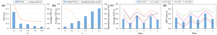
Figure 4. (a) Impact of $\eta$ on PST and average TAT on Xiaohong. (b) Impact of $\gamma$ on average TAT and standard deviation of TAT on the noise model. (c) Impact of $\alpha$ and $\beta$ on average TAT on the noise model ($\gamma=0.5$). (d) Impact of $\alpha$ and $\beta$ on QPU time on the noise model ($\gamma=0.5$). The blue bar in (c) and (d) corresponds with the hyperparameters we pick for the noise model.

4.2. Results on a Simulated Noise Model

As shown in Tbl. 1, our method achieves the shortest average turnaround time (TAT) across all methods. It reduces TAT of Default by nearly 70 percent, which will significantly cut down the waiting time for users to obtain their results. Also, the standard deviation of TAT of our method is the smallest, having a reduction of 60.61% over Default. Small standard deviation means TAT of different users will not differ too much, which showcases the fairness of our algorithm. Our QPU time is the second shortest (a bit longer than SNSF), which attains 51.86% reduction over Default. The PST reduction of our method is only 2.47%. Hence, our method can achieve significant improvements in QPU time and TAT at a trivial cost of fidelity.

Compared with other methods, our method is superior in QPU time and TAT. Three greedy baselines share similar TRF and PST with our method. Though QuMC can ensure high PST (positive $\Delta$PST due to randomness), the QPU time and TAT are about twice longer than our method. The improvements of QuMC in time metrics over Default is rather limited.

4.3. Results on a Quantum Computer

As shown in Tbl. 1, the performance of our method is even better on the quantum processor Xiaohong. We still achieve the shortest average TAT, significantly decreasing TAT of Default by 93.2%. SNSF achieves the shortest QPU time as expected, while the maximum and standard deviation of TAT of ESTF are the lowest, indicating the fairness of ESTF. Among all methods, our method has the second lowest QPU time (81.76% reduction over Default) and standard deviation of TAT (87.31% reduction over Default). Hence, our method can significantly reduce time overhead for both users and suppliers, and meanwhile ensure enough fairness.

The superiority of our method on Xiaohong owes to the large TRF (7.18) and our queue rearranging. With 66 physical qubits, Xiaohong can accommodate more programs in each execution. Hence, the execution times are largely diminished compared to Default, resulting in shorter QPU time and TAT. In addition, our priority score can perceive the potential influence of each job on time metrics, arranging those highly influential programs to the head of the queue. Hence, QPU time and TAT are further reduced.

PST on Xiaohong is much lower in general, because noise on Xiaohong is more severe than on the noise model. Our method has 5.17% reduction in PST over Default, slightly bigger than QuMC (3.81%). However, TRF of QuMC is only 1.98. Hence, its QPU Time and average TAT are 3.4$\times$ and 6.0$\times$ longer than ours. Huge growth in execution latency for a small improvement in fidelity is unworthy.

4.4. Runtime Analysis

As shown in Tbl. 1, the runtime (RT) of our method is close to Default and three greedy baselines. Since routing occupies most of the runtime, our method will not introduce much additional overhead. QuMC costs much more time than us, especially on Xiaohong, because it will repeat routing if a program is unsuitable for its strategy. The runtime of QuMC increases dramatically with the growth in the number of physcal qubits, while our method avoids this issue, indicating the scalability of our method. Note that our scheduling algorithm can run in a pipelining manner with the circuit execution. Hence, it will not affect the running of QPU.

4.5. Sensitivity Analysis

We study the impact of four hyperparameters, i.e. width weight $\alpha$, shot weight $\beta$, time weight $\gamma$, and maximum usage $\eta$. The sensitivity tests for $\alpha$, $\beta$, and $\gamma$ are implemented on the noise model, while the test for $\eta$ is done on Xiaohong, because $\eta$ is more related with PST, and PST on Xiaohong reflects the realistic effect on QPUs.

Time weight $\gamma$. As shown in Fig. 4b, with the increase of $\gamma$, the standard deviation of TAT is getting smaller while average TAT is getting longer. Hence, there is a trade-off between fairness and time metrics. Since time metrics are more important for both users and suppliers, we pick $\gamma=0.5$ in our experiments.

Width weight $\alpha$ and shot weight $\beta$. $\alpha$ and $\beta$ are more concerned with TAT and QPU time. As shown in Fig. 4c and Fig. 4d, the increase in $\alpha$ leads to decline in average TAT and rise in QPU time. By contrast, larger $\beta$ reduces QPU time, and average TAT reaches its minimum when $\beta=2$. To strike a balance between average TAT and QPU time, we pick $\alpha=3,\beta=2$ for the noise model.

Maximum usage $\eta$. It directly influences TRF. As shown in Fig. 4a, with its increase, both average TAT and PST decline. Because more programs are executed in parallel. Hence, we can balance the fidelity and execution latency by tuning $\eta$ and we set $\eta=5/6$.

In general, our method is robust to these hyperparameters.

4.6. Ablation Study of EPST^∗

To evaluate our $EPST^{*}$ score, we execute the candidate circuits through the serial execution mode with and without $EPST^{*}$. For the noise model, $EPST^{*}$ raises PST by 1.59% (from 72.22% to 73.81%). For Xiaohong, it raises PST by 0.94% (from 17.73% to 18.67%). Low PST on Xiaohong is due to its fluctuating noise. Hence, $EPST^{*}$ can improve the fidelity of quantum programs.

5. Conclusion

We have formulated the Quantum Program Scheduling Problem to boost the execution efficiency of (superconducting) quantum processors. Our scheduling method perceives the impact of different programs on time metrics through our priority score, and the noise-aware initial mapping improves the fidelity. Also, three greedy baselines are given for comparison. Results show that our method outperforms greedy baselines in both QPU time and TAT. Besides, the fidelity and fairness are also guaranteed. The small runtime overhead shows its scalability on large QPUs. We envision that our scheduling method may be further adapted to non-superconducting quantum cloud, which we leave for future work.

- (1)
- Aleksandrowicz et al. (2019) Gadi Aleksandrowicz, Thomas Alexander, Panagiotis Barkoutsos, Luciano Bello, Yael Ben-Haim, David Bucher, F Jose Cabrera-Hernández, Jorge Carballo-Franquis, Adrian Chen, Chun-Fu Chen, et al. 2019. Qiskit: An open-source framework for quantum computing. Accessed on: Mar 16 (2019).
- Arute et al. (2019) Frank Arute, Kunal Arya, Ryan Babbush, Dave Bacon, Joseph C Bardin, Rami Barends, Rupak Biswas, Sergio Boixo, Fernando GSL Brandao, David A Buell, et al. 2019. Quantum supremacy using a programmable superconducting processor. Nature 574, 7779 (2019), 505–510.
- Cao et al. (2023) Sirui Cao, Bujiao Wu, Fusheng Chen, Ming Gong, Yulin Wu, Yangsen Ye, Chen Zha, Haoran Qian, Chong Ying, Shaojun Guo, et al. 2023. Generation of genuine entanglement up to 51 superconducting qubits. Nature 619, 7971 (2023), 738–742.
- Cerezo et al. (2021) Marco Cerezo, Andrew Arrasmith, Ryan Babbush, Simon C Benjamin, Suguru Endo, Keisuke Fujii, Jarrod R McClean, Kosuke Mitarai, Xiao Yuan, Lukasz Cincio, et al. 2021. Variational quantum algorithms. Nature Reviews Physics 3, 9 (2021), 625–644.
- Computing (2019) IBM Quantum Computing. 2019. Retrieved Nov 10, 2023 from https://www.ibm.com/quantum.
- Das et al. (2019) Poulami Das, Swamit S Tannu, Prashant J Nair, and Moinuddin Qureshi. 2019. A case for multi-programming quantum computers. In Proc. of MICRO. 291–303.
- Farhi et al. (2014) Edward Farhi, Jeffrey Goldstone, and Sam Gutmann. 2014. A quantum approximate optimization algorithm. arXiv preprint arXiv:1411.4028 (2014).
- Grover (1996) Lov K Grover. 1996. A fast quantum mechanical algorithm for database search. In Proc. of STOC. 212–219.
- Li et al. (2019) Gushu Li, Yufei Ding, and Yuan Xie. 2019. Tackling the qubit mapping problem for NISQ-era quantum devices. In Proc. of ASPLOS. 1001–1014.
- Liu and Dou (2021) Lei Liu and Xinglei Dou. 2021. Qucloud: A new qubit mapping mechanism for multi-programming quantum computing in cloud environment. In 2021 IEEE HPCA. IEEE, 167–178.
- Newman (2004) Mark EJ Newman. 2004. Fast algorithm for detecting community structure in networks. Physical review E 69, 6 (2004), 066133.
- Nielsen and Chuang (2010) Michael A Nielsen and Isaac L Chuang. 2010. Quantum computation and quantum information. Cambridge university press.
- Niu et al. (2020) Siyuan Niu, Adrien Suau, Gabriel Staffelbach, and Aida Todri-Sanial. 2020. A hardware-aware heuristic for the qubit mapping problem in the nisq era. IEEE TQE 1 (2020), 1–14.
- Niu and Todri-Sanial (2023) Siyuan Niu and Aida Todri-Sanial. 2023. Enabling multi-programming mechanism for quantum computing in the NISQ era. Quantum 7 (2023), 925.
- Platform (2022) QuantumCTek Quantum Cloud Platform. 2022. Retrieved Nov 15, 2023 from https://quantumctek-cloud.com/.
- Preskill (2018) John Preskill. 2018. Quantum computing in the NISQ era and beyond. Quantum 2 (2018), 79.
- Resch et al. (2021) Salonik Resch, Anthony Gutierrez, Joon Suk Huh, Srikant Bharadwaj, Yasuko Eckert, Gabriel Loh, Mark Oskin, and Swamit Tannu. 2021. Accelerating variational quantum algorithms using circuit concurrency. arXiv:2109.01714 (2021).
- Shor (1994) Peter W Shor. 1994. Algorithms for quantum computation: discrete logarithms and factoring. In Proc. of FOCS. Ieee, 124–134.
- Siraichi et al. (2018) Marcos Yukio Siraichi, Vinícius Fernandes dos Santos, Caroline Collange, and Fernando Magno Quintão Pereira. 2018. Qubit allocation. In Proc. of CGO. 113–125.
- Soeken et al. (2012) Mathias Soeken, Stefan Frehse, Robert Wille, and Rolf Drechsler. 2012. Revkit: a Toolkit for reversible circuit design. J. Multiple Valued Log. Soft Comput. (2012).
- Tannu and Qureshi (2019) Swamit S Tannu and Moinuddin K Qureshi. 2019. Not all qubits are created equal: A case for variability-aware policies for NISQ-era quantum computers. In Proc. of ASPLOS. 987–999.