Supernova remnants of red supergiants: from barrels to Cygnus-loops

Core-collapse supernova remnants are the nebular leftover of defunct massive stars which have died during a supernova explosion, mostly while undergoing the red supergiant phase of their evolution. The morphology and emission properties of those remnants are a function of the distribution of circumstellar material at the moment of the supernova, the intrisic properties of the explosion, as well as those of the ambient medium. By means of 2.5-dimensional numerical magneto-hydrodynamics simulations, we model the long-term evolution of supernova remnants generated by runaway rotating massive stars moving into a magnetised interstellar medium. Radiative transfer calculations reveal that the projected non-thermal emission of the supernova remnants decreases with time, i.e. older remnants are fainter than younger ones. Older ($80\,\rm kyr$) supernova remnants whose progenitors were moving with space velocity corresponding to a Mach number $M=1$ ($v_{\star}=20\,\rm km\,\rm s^{-1}$) in the Galactic plane of the ISM ($n_{\rm ISM}=1\,\rm cm^{-3}$) are brighter in synchrotron than when moving with a Mach number $M=2$ ($v_{\star}=40\,\rm km\,\rm s^{-1}$). We show that runaway red supergiant progenitors first induce an asymmetric non-thermal $1.4\,\rm GHz$ barrel-like synchrotron supernova remnants (at the age of about $8\,\rm kyr$), before further evolving to adopt a Cygnus-loop-like shape (at about $80\,\rm kyr$). It is conjectured that a significative fraction of supernova remnants are currently in this bilateral-to-Cygnus-loop evolutionary sequence, and that this should be taken into account in the data interpretation of the forthcoming Cherenkov Telescope Array (CTA) observatory.

1 Introduction

Supernova remnants are chemically enriched nebulae made of gas and dust, left behind the explosive death of particular stellar objects, which do not eventually become a white dwarf or collapse as a black hole. In the case of high-mass ($\geq 8\rm M_{\odot}$) progenitors, the mechanism producing the explosion is the so-called core-collapse process (Woosley & Weaver, 1986; Woosley et al., 2002; Smartt, 2009; Langer, 2012), releasing mass and energies (Sukhbold et al., 2016) into the circumstellar nebula that was shaped by the spectacular stellar wind-interstellar medium (ISM) interaction at work prior to it (Weaver et al., 1977; Gull & Sofia, 1979; Chevalier & Liang, 1989; Wilkin, 1996; Bear & Soker, 2021). Hence, the morphological and emission characteristics of supernova remnants are a function of the past evolution of their progenitor that strongly imprint their circumstellar medium as they later channel the propagation of the supernova shock wave as the remnant becomes larger and older, for both high-mass (Kesteven & Caswell, 1987; Wang & Mazzali, 1992; Vink et al., 1996; Uchida et al., 2009) and low-mass (Vink et al., 1997; Vink, 2012; Williams et al., 2013; Broersen et al., 2014). To understand their observed non-thermal emission and to constrain the feedback of supernova remnants from massive stars into the ISM of the Milky Way, it is necessary to first understand in detail their shape. This medium can only be probed by numerical simulations.

Table 1: List of numerical models. All simulations assume a rotating massive progenitor of zero-age main-sequence mass $M_{\star}$ (in $\rm M_{\odot}$) at solar metallicity and moving with velocity $v_{\star}$ through the warm phase of the Galactic plane. The table indicates the stellar evolution history in each model from the MS (main-sequence) phase to the final SN (supernova) explosion and ultimate PWN (pulsar wind) through the RSG (red supergiant) and WR (Wolf-Rayet) stages.

${\rm{Model}}$	$M_{\star}$  ($\rm M_{\odot}$)	$v_{\star}$ ($\rm\,km\,\rm s^{-1}$)	Evolution history
Run-20-MHD-20-SNR	20	20	$\rm MS\rightarrow\rm RSG\rightarrow\rm SN$
Run-20-MHD-40-SNR	20	40	$\rm MS\rightarrow\rm RSG\rightarrow\rm SN$
Run-35-MHD-20-SNRa	35	20	$\rm MS\rightarrow\rm RSG\rightarrow\rm WR\rightarrow\rm SN$
Run-35-MHD-40-SNRa	35	40	$\rm MS\rightarrow\rm RSG\rightarrow\rm WR\rightarrow\rm SN$
(a) Meyer et al. (2023)

The realistic modelling of global supernova remnants through (magneto-)hydrodynamical simulations is, therefore a two-step procedure: first, the wind-ISM interaction must be calculated, and, secondly, the supernova explosion must be realised in it and their interaction subsequently simulated. Examples of solutions for supernova remnants of low-mass progenitors can be found in the studies of Orlando et al. (2007); Petruk et al. (2009); Vigh et al. (2011); Chiotellis et al. (2012, 2013, 2020, 2021). Simulations of remnants of high-mass progenitors are presented in the studies of Orlando et al. (2007); van Marle et al. (2010); Orlando et al. (2012, 2019, 2020, 2021). Among the many degrees of freedom of the parameter space that is controlling the morphologies of core-collapse supernova remnants, the supersonic motion that is affecting a significant fraction of massive stars, i.e., of core-collapse progenitors, is a preponderant element to account for in the understanding of asymmetric supernova remnants (Bear & Soker, 2017; Meyer et al., 2020, 2023) and its influence continues up to the pulsar wind nebulae developing in plerion, the remnants of high-mass progenitors in which a neutron star forms (Meyer et al., 2023). Interestingly, the peculiar radio emission of barrel-like and horseshoe supernova remnants can be explained by invoking the coupling of the stellar wind history with the bulk motion of a progenitor undergoing a Wolf-Rayet phase before exploding (Meyer et al., 2021b).

Core-collapse supernova remnants have been observed by means of both their thermal and non-thermal emission and the mass of their progenitor constrained in Katsuda et al. (2018), although their classification remains open (Soker & Kaplan, 2021; Soker, 2023a, b; Shishkin & Soker, 2023). This study shows that an exploding red supergiant star might generate most of such remnants. These stars shape the stellar surroundings at the pre-supernova time in a particular manner, which is a key question to understand (Soker, 2021). A noticeable example is the Cygnus-Loop nebulae, whose peculiar morphology may arise from the interaction of a supernova shock wave with the walls of a cavity carved by the stellar wind of a defunct runaway red supergiant star (Fang et al., 2017). A deeper understanding of the internal functioning of such remnants requires an additional numerical effort, bringing together higher spatial resolution, stellar rotation, and magnetisation of the cold pre-supernova wind, as well as a better post-processing of the results to extract synchrotron emission maps to be directly compared with real observations. This is of great interest, especially for the Cherenkov Telescope Array, see Acharyya et al. (2023); Acero et al. (2023); Cherenkov Telescope Array Consortium et al. (2023).

In this paper, we continue our numerical exploration of the morphologies and non-thermal synchrotron emission properties of core-collapse supernova remnants of runaway massive stars, that has been initiated in Meyer et al. (2023) by means of 2.5-dimensional magneto-hydrodynamical simulations. This paper focuses on the comparison between supernova remnants of zero-age main-sequence $20\,\rm M_{\odot}$ exploding while undergoing a red supergiant, and compared to supernova remnants of zero-age main-sequence $35\,\rm M_{\odot}$ finishing their life as a Wolf-Rayet star. We generate $1.4\,\rm GHz$ synchrotron emission maps using the method developed in Villagran et al. (2024), which allows recovery of the physical units of the projected emissions that are often presented in a normalised fashion. It is, therefore, possible to compare the brightnesses of the modelled supernova remnants as a function of time and of the initial conditions of the simulations. The synthetic emission maps are compared and discussed with real observations of supernova remnants.

The paper is organised as follows. In Section 2, we introduce the reader to the numerical methods used to generate the results detailed in Section 3. We further discuss the results in this study in Section 4 and conclude in Section 5.

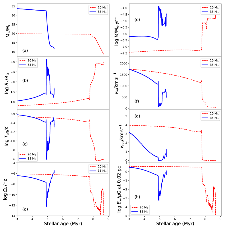
Figure 1: Temporal evolution (in $\rm Myr$) of the supernova progenitors of zero-age main-sequence $20\,\rm M_{\odot}$ (dotted red line) and $35\,\rm M_{\odot}$ (solid blue line) considered in our study. The panels display the stellar mass $M_{\star}$ (panel a, in $\rm M_{\odot}$), radius $R_{\star}$ (panel b, in $\rm R_{\odot}$), effective temperature $T_{\rm eff}$ (panel c, in $\rm K$), angular frequency at the surface $\Omega_{\star}$ (panel d, in $\rm Hz$), mass-loss rate $\dot{M}$ (panel e, in $\rm M_{\odot}\,\rm yr^{-1}$), wind velocity $v_{\rm w}$ (panel f, in $\rm km\ \rm s^{-1}$), equatorial rotation velocity $v_{\rm rot}$ (panel g, in $\rm km\ \rm s^{-1}$), the magnetic field in the wind at $0.02\,\rm pc$ $B_{\star}$ (panel h, in $\mu\rm G$).

2 Method

In this section, we present the boundary and initial conditions of the magneto-hydrodynamical simulations performed in this study. It details the stellar evolution models utilised, the used calculation strategy, numerical methods and the assumptions adopted for the radiative transfer calculations in order to compare our results with real observations.

2.1 Interstellar medium

The assumed ISM number density is taken as $n_{\rm ISM}=0.79\,\rm cm^{-3}$, which corresponds to that of the warm phase of the Galactic plane (Wolfire et al., 2003). The gas is assumed to be ionized and has a temperature of $T_{\,\rm ISM}=8000\,\rm K$ (Meyer et al., 2023). Its magnetic field of strength $B_{\rm ISM}=7\,{\rm\mu G}$ (Meyer et al., 2024) is considered as uniform and organised linearly, parallel to the direction of motion of the star. This configuration is imposed by the two-dimensional nature of the calculations, see van Marle et al. (2015); Meyer et al. (2017). The gas is initially in equilibrium between the cooling of the material at high temperature and the heating provided by the starlight, which ionises the circumstellar gas.

The heating rate $\Gamma$ stands for the recombining hydrogenoic ions that are ionized by photospheric photons. The liberated electrons get the quantum of energy transported by the ionizing photon. This process happens at a rate that is taken from the recombination coefficient $\alpha_{\mathrm{rr}}^{\mathrm{B}}$, interpolated from the table 4.4 of Osterbrock (1989). The cooling term $\Lambda$ includes contributions from H, He and metals at solar helium abundance $Z$ (Wiersma et al., 2009; Asplund et al., 2009), modified to include the H recombination line cooling by use of the energy loss coefficient case B of Hummer (1994) and the O and C forbidden lines by collisionally excited emission presented in Henney et al. (2009). Our study uses species abundance at $\rm O/\rm H=4.89\times 10^{-4}$ in number density (Asplund et al., 2009).

2.2 Magnetized, rotating stellar wind

The stellar wind terminal radial velocity is calculated as,

$$v_{\rm w}(t)=\sqrt{\beta(T)\frac{2GM_{\star}(t)}{R_{\star}(t)}},$$ (1)

where $G$ is the gravitational constant, $M_{\star}$ the stellar mass and $R_{\star}$ the stellar radius, respectively. The factor $\beta(T)$ is a piece-wise function of the temperature that is taken from the study of Eldridge et al. (2006). In this study, as in the former work of this series (Meyer et al., 2023), the escape wind velocity is calculated using the photospheric luminosity and the effective temperature to compute the stellar radius and, therefore, wind terminal speed. This reduces values for the Wolf-Rayet pĥase (at $5.33\,\rm Myr$ after the zero-age main sequence). The physics for the terminal wind velocity of WR stars is not well understood, and our values are still largely in accordance with observations of weak-winded ($<1000\,\rm km\,\rm s^{-1}$) Galactic Wolf-Rayet stars e.g. WR16, WR40, WR105 (Hamann et al., 2019). The radial-dependence of the stellar wind density reads,

$$\rho_{w}(r,t)=\frac{\dot{M}(t)}{4\pi r^{2}v_{\rm w}(t)},$$ (2)

with $\dot{M}$ the mass-loss rate of the massive star at a given time $t$.

We consider massive stars, which, at the onset of their main sequence, initially rotate such that,

$$\frac{\Omega_{\star}(t=0)}{\Omega_{\rm K}}=0.1,$$ (3)

and with,

$$\Omega_{\star}(t)=\frac{v_{\rm rot}(t)}{R_{\star}(t)},$$ (4)

where $\Omega_{\star}$ and $\Omega_{\rm K}$ are the equatorial and Keplerian rotational velocities, respectively, and $v_{\rm rot}$ the toroidal velocity. The latitude-dependent toroidal component of the rotation surface is, therefore,

$$v_{\phi}(\theta,t)=v_{\rm rot}(t)\sin(\theta),$$ (5)

while its polar component is set to $v_{\theta}=0$, see also the 2.5-dimensional approach developed for the modelled magnetised wind of rotating stars in  Parker (1958); Weber & Davis (1967); Pogorelov & Semenov (1997); Pogorelov & Matsuda (2000); Chevalier & Luo (1994); Rozyczka & Franco (1996).

The other characteristic stellar parameters are interpolated from the tabulated evolution models from the geneva library  (Eggenberger et al., 2008; Ekström et al., 2012), which provides the evolutionary structure and effective surface properties of high-mass stars from their zero-age main-sequence mass to their pre-supernova time when the Si burning phases happen. Our model, therefore, assumes that the mass-loss rate and the radial component of the wind velocity of the progenitor star are spherically symmetric throughout its entire pre-supernova evolution. Such an approach is typical and finds its origins in the early developments of stellar evolution codes (Heger et al., 2000; Eggenberger et al., 2008; Brott et al., 2011a, b; Ekström et al., 2012), treating the hydrodynamic stellar structure equations for massive stars in a 1D-dimensional fashion as long they do not rotate close to their critical angular velocity (Georgy et al., 2011), and it is supported by observations of massive star’s stellar wind close to the termination shock of their pc-scale nebulae (Weaver et al., 1977; van Buren & McCray, 1988; Wilkin, 1996; Peri et al., 2012, 2015), also leading to a spherically symmetric theory for hot-star wind acceleration driven by line-emission and radiation pressure (Abbott, 1980, 1982; Friend & Abbott, 1986). However, many factors, such as binarity, affecting up to $70\%$ of massive stars, impose azimuthal deviations to these winds, especially in the region in the vicinity of the orbital plane of massive multiple system (Sana et al., 2012). Additionally, the alternation of high and slow winds at the phase transitions like the onset of the red supergiant, blue supergiant or Wolf-Rayet evolutionary sequences are also a source of asymmetry (Parkin et al., 2011; Madura et al., 2013; Gvaramadze et al., 2015; Martayan et al., 2016; El Mellah et al., 2020). Since we concentrate on the large-scale surroundings of single, slowly-rotating objects, the spherically symmetric assumption for stellar winds is acceptable. For completeness, the Hertzsprung-Russel diagram of the two progenitor stars we consider in this study is plotted in Fig. 2.

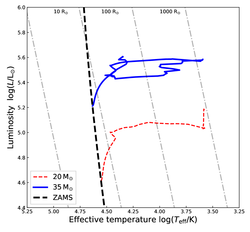
Figure 2: Evolutionary tracks in the Hertzsprung-Russell-diagram of the two progenitor stars of initial masses $20\,\rm M_{\odot}$ (dotted red) and $35\,\rm M_{\odot}$ (solid blue) considered in this study (Ekström et al., 2012).

The stellar magnetic field structure is assumed to be a Parker spiral,

$$B_{\rm r}(r,t)=B_{\star}(t)\Big{(}\frac{R_{\star}(t)}{r}\Big{)}^{2},$$ (6)

$$B_{\phi}(r,t)=B_{\rm r}(r,t)\left(\frac{v_{\phi}(\theta,t)}{v_{\rm w}(t)}\right)\left(\frac{r}{R_{\star}(t)}-1\right),$$ (7)

and

$$B_{\theta}(r,t)=0$$ (8)

respectively. The total stellar wind magnetic field therefore reads,

$$B_{\rm w}(r,t)=\sqrt{B_{\rm r}(r,t)^{2}+B_{\phi}(r,t)^{2}+B_{\theta}(r,t)^{2}}.$$ (9)

The magnetic field strength at the surface of the star is scaled to that of the Sun, as described in Scherer et al. (2020); Herbst et al. (2020); Baalmann et al. (2020, 2021); Meyer et al. (2021a). We adopt the time-dependent evolution of the surface magnetic field $B_{\star}$ of the supernova progenitor as derived in Meyer et al. (2023, 2024). The main-sequence surface magnetic field strength is taken to $B_{\star}=500\,\rm G$ (Fossati et al., 2015; Castro et al., 2015; Przybilla et al., 2016; Castro et al., 2017), the red supergiant phase one to that of Betelgeuse, i.e. $B_{\star}=0.2\,\rm G$ (Vlemmings et al., 2002, 2005; Kervella et al., 2018), while for the Wolf-Rayet phase we assume $B_{\star}=100\,\rm G$ (Hubrig et al., 2016; de la Chevrotière et al., 2014; Meyer, 2021).

2.3 Supernova ejecta

The supernova blastwave, whose properties are determined by the mass of the ejecta $M_{\rm ej}$ and energy of the explosion $E_{\rm ej}$ (Shishkin & Soker, 2023), is modelled using the method of Truelove & McKee (1999). The blastwave is injected at the time of the explosion considering the following radial density profile,

$$\rho(r)=\begin{cases}\rho_{\rm core}(r)&\text{if $r\leq r_{\rm core}$},\\ \rho_{\rm max}(r)&\text{if $r_{\rm core}<r<r_{\rm max}$},\\ \end{cases}$$ (10)

with an inner constant region, the so-called core, characterised by a density,

$$\rho_{\rm core}(r)=\frac{1}{4\pi n}\frac{(10E_{\rm ej}^{n-5})^{-3/2}}{(3M_{\rm ej}^{n-3})^{-5/2}}\frac{1}{t_{\rm max}^{3}},$$ (11)

and an outer steeply decreasing region of density

$$\rho_{\rm max}(r)=\frac{1}{4\pi n}\frac{\left(10E_{\rm ej}^{n-5}\right)^{(n-3)/2}}{\left(3M_{\rm ej}^{n-3}\right)^{(n-5)/2}}\frac{1}{t_{\rm max}^{3}}\bigg{(}\frac{r}{t_{\rm max}}\bigg{)}^{-n},$$ (12)

where the exponent $n=11$ is typical for massive progenitor stars (Chevalier & Liang, 1989) and where $r_{\rm max}$ is the outer limit of the blastwave at that time. The age of the blastwave is determined using the iterative procedure of Whalen et al. (2008), such that,

$$t_{\rm max}=\frac{r_{\rm max}}{v_{\rm max}},$$ (13)

with $v_{\rm max}=3\times 10^{4}\,\rm km\,\rm s^{-1}$.

The velocity profile of the blastwave is taken as,

$$v(r)=\frac{r}{t},$$ (14)

which ensures that the early blastwave propagates homologously in the pre-supernova stellar wind of the progenitor. The ejecta velocity at a distance $r_{\rm core}$ from the center of the explosion reads,

$$v_{\rm core}=\bigg{(}\frac{10(n-5)E_{\rm ej}}{3(n-3)M_{\rm ej}}\bigg{)}^{1/2},$$ (15)

see  Truelove & McKee (1999); Whalen et al. (2008); van Veelen et al. (2009); van Marle et al. (2010). The mass of defunct stellar material in the supernova ejecta is determined by subtracting the mass of a neutron star $M_{\mathrm{NS}}=1.4\,\rm M_{\odot}$ to that of the progenitor at the moment of the explosion,

$$M_{\rm ej}=M_{\star}-\int_{t_{\mathrm{ZAMS}}}^{t_{\mathrm{SN}}}\dot{M}(t)\leavevmode\nobreak\ dt-M_{\mathrm{NS}},$$ (16)

which is $7.28\,\rm M_{\odot}$ and $10.12\,\rm M_{\odot}$ for the $20\,\rm M_{\odot}$ and $35\,\rm M_{\odot}$ progenitors, respectively.

Our setting of the supernova blastwave assumes spherical symmetry of the radial component of the supernova ejecta. This is a classical approach to numerical simulations like ours (van Veelen et al., 2009; van Marle et al., 2010), consisting of considering that the homologous expansion of the supernova material through the last stellar wind is not affected by any latitude- or azimuthal-dependent hydrodynamical flow. One should mention that the physics of core-collapse supernova explosion is complex and far beyond the simple prescription used in this study. Particularly the anisotropic in the emission of a released neutrino can greatly change the explosion energy and channel it in the direction of the neutrino anisotropies, producing anisotropic blastwave (Shimizu et al., 2001; Müller et al., 2012; Gabler et al., 2021). Furthermore, the presence of a binary companion leads to additional blastwave-circumstellar interactions potentially producing so-called common envelope jets supernova in which a first component explodes, giving a compact object (black hole or neutron star) that accretes material from its post-main-sequence companion, such as a supergiant star (Papish & Soker, 2011, 2014; Gilkis et al., 2016; Bear & Soker, 2018; Kaplan & Soker, 2020; Soker, 2022a, b, c, 2023a). Since our work considers single stars explosion of the canonical energy of $10^{51}\,\rm erg$, we neglect any anisotropy in the supernova blastwave and/or jet pushing out the gas of a former common envelope.

2.4 Governing equations

The equations solved on the grid meshing the computational domain are those of the non-ideal magneto-hydrodynamics. They read as,

$$\frac{\partial\rho}{\partial t}+\@vec{\nabla}\cdot\big{(}\rho\@vec{v})=0,$$ (17)

$$\frac{\partial\@vec{m}}{\partial t}+\@vec{\nabla}\cdot\Big{(}\@vec{m}\otimes\@vec{v}-\@vec{B}\otimes\@vec{B}+\@vec{\hat{I}}p_{\rm t}\Big{)}=\@vec{0},$$ (18)

$$\frac{\partial E}{\partial t}+\@vec{\nabla}\cdot\Big{(}(E+p_{\rm t})\@vec{v}-\@vec{B}(\@vec{v}\cdot\@vec{B})\Big{)}=\Phi(T,\rho),$$ (19)

$$\frac{\partial\@vec{B}}{\partial t}+\@vec{\nabla}\cdot\Big{(}\@vec{v}{\color[rgb]{0,0,0}\otimes}\@vec{B}-\@vec{B}{\color[rgb]{0,0,0}\otimes}\@vec{v}\Big{)}=\@vec{0},$$ (20)

where $\rho$ is the mass density, $\@vec{v}$ the vector velocity, $\@vec{m}$ the vector momentum, and $\@vec{B}$ the vector magnetic field, respectively. In the above relations, $\@vec{\hat{I}}$ is the identity vector, $\@vec{0}$ is the null vector, and $p_{\rm t}$ is the total pressure (thermal $p$ plus magnetic $B^{2}/8\pi$ ) of the gas. The total energy of the gas reads,

$$E=\frac{p}{(\gamma-1)}+\frac{\@vec{m}\cdot\@vec{m}}{2\rho}+\frac{\@vec{B}\cdot\@vec{B}}{8\pi},$$ (21)

and the system is closed with the relation,

$$c_{\rm s}=\sqrt{\frac{\gamma p}{\rho}},$$ (22)

with $c_{\rm s}$ the sound speed of the gas, with $\gamma$ the adiabatic index.

The right-hand side term,

$$\Phi(T,\rho)=n_{\mathrm{H}}\Gamma(T)-n^{2}_{\mathrm{H}}\Lambda(T),$$ (23)

of Eq.19 represents the losses and heating by optically-thin radiative processes. The H gas number density is,

$$n_{\mathrm{H}}=\frac{\rho}{\mu(1+\chi_{\rm He,Z})m_{\mathrm{H}}},$$ (24)

with $\mu$ the mean molecular weight, $\chi_{\rm He,Z}$ the He and metals (species of atomic number larger or equal to 2) and $m_{\mathrm{H}}$ the proton mass, respectively, and

$$T=\mu\frac{m_{\mathrm{H}}}{k_{\rm{B}}}\frac{p}{\rho},$$ (25)

is the temperature of the gas.

2.5 Synchrotron emission calculation

Our study aims to investigate the radio appearance of the supernova remnants. To this end, let us first call the relativistic electron energy distribution,

$$N(\gamma)=K\gamma^{-p}\propto\gamma^{-p},$$ (26)

with $K$ a proportionality constant, $p$ an index function of the spectral index via $p=2\alpha+1$ and $\gamma$ the Lorentz factor,

$$\gamma=\frac{E}{E_{0}}=\frac{\gamma m_{0}c^{2}}{m_{0}c^{2}},$$ (27)

with $m_{0}$ the rest mass of the electrons and $c$ the speed of light.

The synchrotron emissivity at a frequency $\nu$ is defined for a given Lorentz factor range as,

$$\epsilon_{\rm sync}(\nu,\theta)=\frac{1}{4\pi}\int_{\gamma_{1}}^{\gamma_{2}}N(\gamma)P_{\rm sync}(\nu,\gamma,\theta)d\gamma,$$ (28)

with $\gamma_{1}<\gamma_{2}$ which can be, using the Eq. 4.43 in Ghisellini (2013), rewritten as,

$$\epsilon_{\rm sync}(\nu)=\frac{3\sigma_{\rm T}cKU_{\rm B}}{8\pi^{2}\nu_{\rm L}}(\sin{\theta})^{(p+1)/2}\Big{(}\frac{\nu}{\nu_{\rm L}}\Big{)}^{-\frac{p-1}{2}}f_{\rm sync}(p),$$ (29)

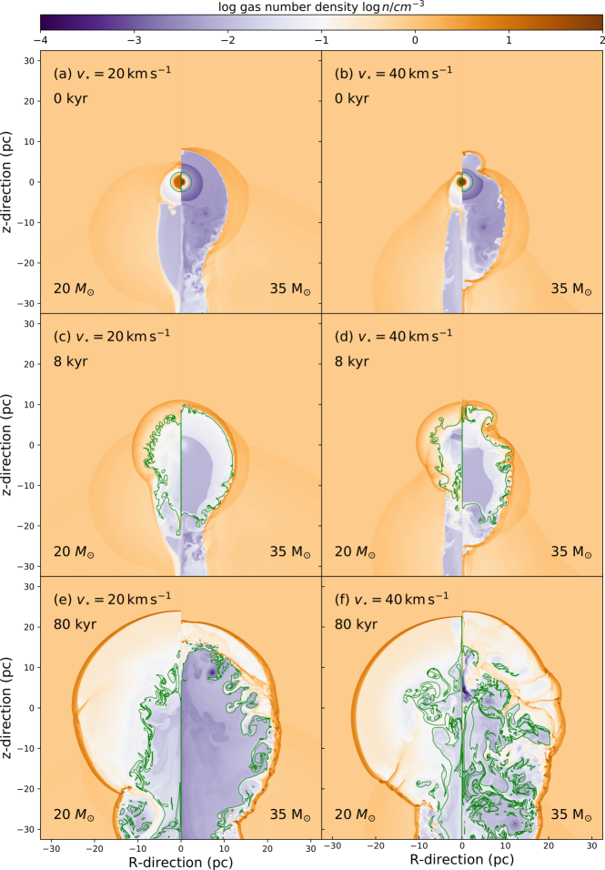
Figure 3: Comparison between the number density fields in the supernova remnant models of a runaway $20\,\rm M_{\odot}$ (left-hand part of the panels) and a $35\,\rm M_{\odot}$ (right-hand part of the panels) star rotating with $\Omega_{\star}/\Omega_{\rm K}=0.1$ and moving with velocity $v_{\star}=20\,\rm km\,\rm s^{-1}$ (left column of panels) and $v_{\star}=40\,\rm km\,\rm s^{-1}$ (right column of panels). The green contour mark the parts of the supernova remnants with a $50\%$ contribution of ejecta.

with $\sigma_{\rm T}$ the Thomson cross section, the special function,

$$f_{\rm sync}(p)=3^{p/2}\frac{\Gamma\Big{(}\frac{3p-1}{12}\Big{)}\Gamma\Big{(}\frac{3p+19}{12}\Big{)}}{p+1}$$ (30)

the magnetic density energy,

$$U_{\rm B}=\frac{B^{2}}{8\pi},$$ (31)

and the Larmor frequency,

$$\nu_{\rm L}=\frac{eB}{2\pi m_{e}c},$$ (32)

where $m_{e}$ is the electron mass.

The local magnetic field strength $B$ in the above relations is substituted by its component normal to the line-of-sight of unit vector $\@vec{l}$ defining the viewing angle of the observer $\theta_{\rm obs}=\angle(\@vec{l},\@vec{B})$. The magnetic total intensity relates to the normal component,

$$B_{\perp}=|\@vec{B}\cdot\@vec{l}|=|\@vec{B}||\@vec{l}|\sin(\theta_{\rm obs})=|\@vec{B}|\sin(\theta_{\rm obs}),$$ (33)

which we express as,

$$B_{\perp}=|\@vec{B}|\sqrt{1-\cos(\theta_{\rm obs})^{2}},$$ (34)

where,

$$|\@vec{B}|=\sqrt{B_{\rm R}^{2}+B_{\rm z}^{2}+B_{\phi}^{2}}.$$ (35)

with $B_{\rm R}$, $B_{\rm z}$ and $B_{\phi}$ its cylindrical components. We need to find the value of $\cos(\theta_{\rm obs})$, that is done via the following vectorial product,

$$|\@vec{B}\times\@vec{l}|=|\@vec{B}||\@vec{l}|\cos(\theta_{\rm obs})=|\@vec{B}|\cos(\theta_{\rm obs}),$$ (36)

or,

$$\cos(\theta_{\rm obs})=\frac{|\@vec{B}\times\@vec{l}|}{|\@vec{B}|},$$ (37)

and, finally, combining Eqs. 34, 37 one obtains,

$$B_{\perp}=|\@vec{B}|\sqrt{1-\Big{(}\frac{|\@vec{B}\times\@vec{l}|}{|\@vec{B}|}\Big{)}^{2}},$$ (38)

respectively. The modulus of the cross product (left-hand side is of Eq. 36) is calculated explicitly with the cylindrical components of $\@vec{B}$ and $\@vec{l}$ expressed in the cylindrical coordinate system of the numerical simulation.

Reminding that both non-thermal electron density and non-thermal electron energy are linked to the plasma number and energy densities with the following relations,

$$x_{\rm n}n=\int_{\gamma_{\rm min}}^{+\infty}K\gamma^{-p}d\gamma\approx\frac{K}{p-1}\gamma_{\rm min}^{-p+1},$$ (39)

and,

$$x_{\rm e}\epsilon_{g}=\int_{\gamma_{min}}^{\infty}K\gamma^{-p}(\gamma-1)m_{e}c^{2}d\gamma,$$ (40)

with $n$ the number density and $\epsilon_{g}$ the energy density of the gas, respectively. The quantities $x_{n}$ and $x_{e}$ are fractions depending on $\gamma_{\rm min}$, with $x_{n}>0$ being related to the injection factor of the accelerated particles and $x_{e}$ a variable related to the non-thermal electrons cooling. Then, one can rewrite Eqs. 39-40 as,

$$x_{\rm e}\epsilon_{g} = \int_{\gamma_{\rm min}}^{+\infty}K\gamma_{e}^{-p}(\gamma_{e}-1)m_{e}c^{2}d\gamma=$$ (41)

$$\simeq m_{e}c^{2}\underbrace{\frac{K}{p-1}\gamma_{\mathrm{min}}^{-p+1}}_{=\chi_{n}n}\bigg{(}\underbrace{\frac{p-1}{p-2}\gamma_{\mathrm{min}}}_{\gg 1}-1\bigg{)},$$ (42)

with,

$$\gamma_{\rm min}=\frac{x_{\rm e}\epsilon_{g}}{x_{\rm n}n}\frac{p-2}{p-1}\frac{1}{m_{e}c^{2}},$$ (43)

and with the above proportionality constant of Eq. 3,

$$K=(p-1)x_{\rm n}n\gamma_{\rm min}^{p-1},$$ (44)

respectively.

The frequency-dependent synchrotron emissivity finally takes the form of,

$$\epsilon_{\rm sync}(\nu)=C_{00}C_{01}\Bigg{(}\frac{(p-1)x_{\rm n}n}{(m_{e}c^{2})^{p-1}}\Bigg{)}(\sin{\theta})^{(p+1)/2}\nu^{-\frac{p-1}{2}}f_{\rm sync}(p),$$ (45)

with the coefficients,

$$C_{00}=\frac{3}{8}\frac{\sigma_{\rm T}c}{\pi^{2}}c\frac{B^{2}}{8\pi}\Big{(}\frac{eB}{2\pi m_{e}c}\Big{)}^{\frac{p-3}{2}},$$ (46)

and,

$$C_{01}=\Big{(}\frac{x_{\rm e}}{x_{\rm n}}\frac{p-2}{p-2}\frac{\epsilon_{g}}{nm_{e}c^{2}}\Big{)}^{p-1},$$ (47)

respectively, which we calculate assuming that $x_{e}$=$x_{n}$=0.1 and $p=2.2$ as in Villagran et al. (2024) .

The intensity emission map at a given frequency $\nu$ is finally generated by projecting the non-thermal emissivity,

$$I_{\rm sync}(\nu)=\int\epsilon_{\rm sync}(\theta_{\rm obs})dl,$$ (48)

to obtain an emission map with an aspect angle $\theta_{\rm obs}$ between the observer’s line of sight and the plane into which the supernova remnant lie.

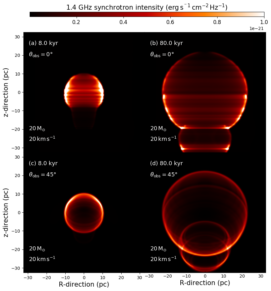
Figure 4: Non-thermal $1.4\,\rm GHz$ synchrotron emission maps (in $\rm erg\,\rm s^{-1}\,\rm cm^{-2}\,\rm sr^{-1},\rm Hz^{-1}$) for the supernova remnant generated by a $M_{\star}=20\,\rm M_{\odot}$ progenitor moving at $v_{\star}=20\,\rm km\,\rm s^{-1}$, respectively. The remnants are shown are times $8\,\rm kyr$ (left panels) and $80\,\rm kyr$ (right panels) after the explosion, with a viewing angle of the observer that is inclined by $\theta=0^{\circ}$ (top panels) and $\theta=45^{\circ}$ (bottom panels) with respect to the plane of the object. The ring-like structures result in the mapping of 2.5-dimensional simulations being mapped into a 3-dimensional shape.

Figure 5: As Fig. 4 for $M_{\star}=35\,\rm M_{\odot}$ progenitor moving with velocity $v_{\star}=20\,\rm km\,\rm s^{-1}$. The ring-like structures result in the mapping of 2.5-dimensional simulations being mapped into a 3-dimensional shape.

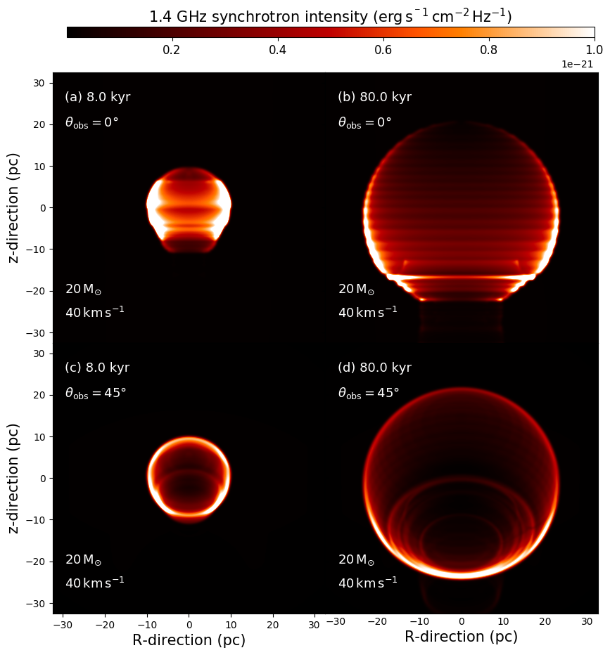
Figure 6: As Fig. 4 for $M_{\star}=20\,\rm M_{\odot}$ progenitor moving with velocity $v_{\star}=40\,\rm km\,\rm s^{-1}$. The ring-like structures result in the mapping of 2.5-dimensional simulations being mapped into a 3-dimensional shape.

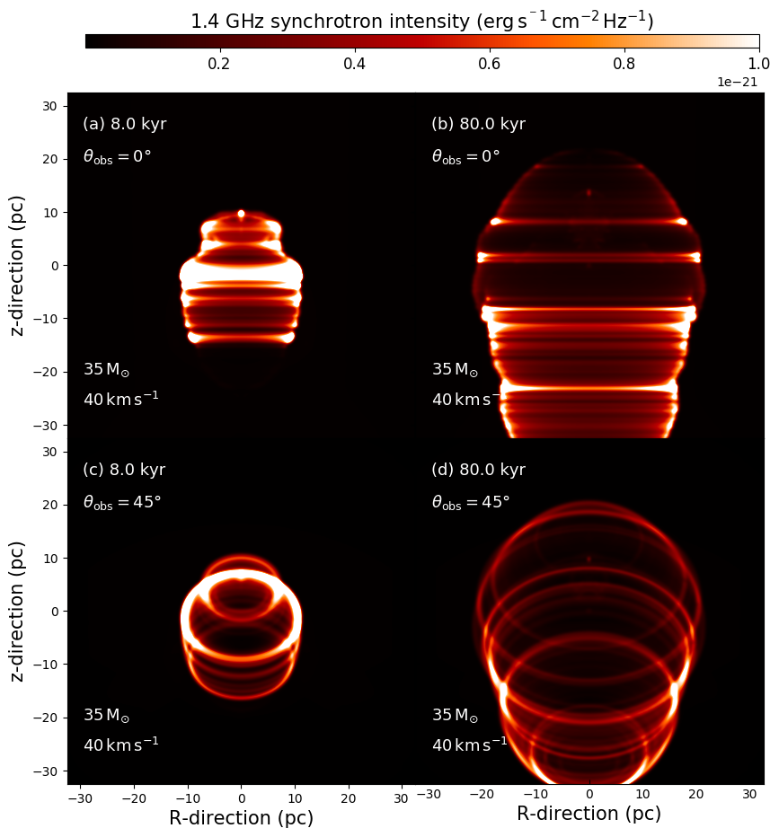
Figure 7: As Fig. 4 for $M_{\star}=35\,\rm M_{\odot}$ progenitor moving with velocity $v_{\star}=40\,\rm km\,\rm s^{-1}$. The ring-like structures result in the mapping of 2.5-dimensional simulations being mapped into a 3-dimensional shape.

2.6 Modelling strategy and numerical methods

This project extends the study of Meyer et al. (2023) to the regime of core-collapse supernova progenitors, which do not undergo a Wolf-Rayet phase but end their lives as a red supergiant star. To this end, it compares the morphologies and non-thermal appearances of their middle-aged to older ($80\ \rm kyr$) supernova remnants. The stellar wind-ISM interaction is first modelled during the entire star’s life, providing the circumstellar medium’s MHD structure, which is later used as initial conditions for the blastwave-surroundings interaction. The progenitor star wind is injected into the computational domain in a circular zone of radius $r_{\rm in}=0.01\,\rm pc$ from the origin. Throughout the simulations, stellar motion is taken into account by setting a velocity $v=-v_{\star}$, being $v_{\star}$ the velocity of the moving star along the direction of the magnetic field lines Meyer et al. (2017). A parameter space of two distinct velocities is explored, namely $v_{\star}=20\,\rm km\,\rm s^{-1}$ and $v_{\star}=40\,\rm km\,\rm s^{-1}$. We summarize the models in this work in Tab 1.

The ejecta-circumstellar medium is calculated in the frame of the moving star in a 2.5-dimensional cylindrical coordinate system (O;R,z) or origin $O$ that includes a toroidal component for each vector, rotational invariant with respect to the axis of symmetry $Oz$. The equations are solved in a computational domain $[0;100]\times[-50;50]\,\rm pc^{2}$ mapped with an uniform mesh of $2000\times 4000$ cells. The numerical simulations are performed using the pluto code (Mignone et al., 2007, 2012; Vaidya et al., 2018) , with a Godunov-type solver made of HLL Rieman solver (Harten et al., 1983), a Runge-Kutta integrator and the divergence-free eight-wave finite-volume algorithm (Powell, 1997), respectively. We refer the reader interested in further details on the numerical scheme and on the limitation of the method to the study of Meyer (2021). The projection of the synchrotron emissivity is perfomed using a modified version of the radiative transfer code radmc-3d, which performs the ray-tracing along a particular line of sight. The physical and characteristic quantities of the supernova progenitors are plotted in Fig. 1.

3 Results

3.1 Supernova remnants morphology

Fig. 3 plots the surroundings of the supernova progenitors considered in this study, at the time of onset of the blastwave propagation and at later times, when it propagates through the wind bubble. In each panel, the left-hand side part refers to the model for the zero-age main sequence $M_{\star}=20\,\rm M_{\odot}$ star, while the right-hand part concerns the $M_{\star}=35\,\rm M_{\odot}$ progenitor star. The simulations are displayed for runaway stars moving with velocity $v_{\star}=20\,\rm km\,\rm s^{-1}$ (left column of panels) and $v_{\star}=40\,\rm km\,\rm s^{-1}$ (right column panels). They represent the number density field (in $\rm cm^{-3}$) in the simulations, onto which a green isocontour marks the regions of the supernova remnants that are made of equal quantities of ejecta and stellar wind material.

In both models, the circumstellar medium has the typical morphology produced around an evolving stellar wind that runs through the ISM, with a bow shock ahead of the direction of stellar motion and a cavity behind it, see Fig. 3a,b). In the early phase of their evolution, the supernova remnants conserve the global appearance of their progenitor’s circumstellar medium since the blastwave has not yet interacted with the stellar surroundings. They are constituted of a large, complex stellar wind bow shock, the result of the interaction of the wind blown by the star throughout the various evolutionary phases of its life (Meyer et al., 2015). The power of stellar winds is stronger for Wolf-Rayet stars than for red supergiant progenitors. Their associated final bow shocks are wider and present large eddies due to Rayleigh-Tayler instabilities in the case of the $M_{\star}=35\,\rm M_{\odot}$ model (Brighenti & D’Ercole, 1995b, a), see Fig. 3a,b. On the contrary in the $M_{\star}=20\,\rm M_{\odot}$ model is much smoother, see studies on the close surroundings of runaway red supergiants (Noriega-Crespo et al., 1997; Decin et al., 2012; Mohamed et al., 2012; Meyer et al., 2021a). Our model raises the question of the nature of the large-scale instabilities developing into the bow shock of the last pre-supernova stellar wind, as it is the first circumstellar structure that the blastwave will encounter when expanding past the snowplough phase. This is particularly pronounced in the supernova remnant generated by a $M_{\star}=35\,\rm M_{\odot}$ progenitor star moving at velocity $v_{\star}=40\,\rm km\,\rm s^{-1}$, of potential numerical origin. This feature develops with our code for the combination of bulk motion and ISM number density that we consider and disappears in the model with lower $v_{\star}$, see Fig. 3a,b, which witness a physical origin in the growth of such Rayleigh-Taylor-based instabilities (Vishniac, 1994; van Marle et al., 2014), however, the role of the symmetry axis of our coordinate system in triggering the instabilities is known and should be kept in mind (Mignone, 2014). Full three-dimensional models of such systems would only permit to answer this question (Blondin & Koerwer, 1998; Meyer et al., 2021a), also exploring the stabilising role of the ambient medium magnetic field on the overall morphology of the supernova remnant and the mixing of material therein.

At $8\,\rm kyr$, the supernova shock wave has reached and interacted with the bow shocks in each model (Fig. 3c,d). Along the direction of stellar motion, one can see the effect of the mass that is trapped into the circumstellar medium, in the sense that the forward shock of the expanding blastwave has gone through the bow shock and propagates further into the unperturbed ISM as a mushroom-like outflow. This process is more important in the case of the supergiant progenitor than that of the $M_{\star}=35\,\rm M_{\odot}$ progenitor (Meyer et al., 2015). At times $80\,\rm kyr$, the reverse shock of the supernova is more advanced in its reverberation towards the centre of the explosion in the simulation with a $M_{\star}=20\,\rm M_{\odot}$ progenitor, due to the small bow shock triggers it sooner. Nevertheless, the unstable character of this inward-moving shock front is more pronounced in the case of the model with a Wolf-Rayet supernova progenitor because the shock surface is wider. The instabilities had more time to grow due to the ejecta-wind strong contrast in density and velocity in the ejecta-circumstellar medium interface (green contours), see Fig. 3e,f.

3.2 Synchrotron emission maps

Fig. 4 shows the $1.4\,\rm GHz$ emission maps of the supernova remnant generated by the moving progenitors with velocity $v_{\star}=20\,\rm km\,\rm s^{-1}$, considering viewing angles of $\theta_{\rm obs}=0^{\circ}$ (top panels) and $\theta_{\rm obs}=45^{\circ}$ (bottom panels), at $8\,\rm kyr$ (left panels) and $80\,\rm kyr$ (right panels) of evolution. These maps correspond to the case of a progenitor with $M_{\star}=20\,\rm M_{\odot}$. The remnant in the model Run-20-MHD-20-SNR, for $\theta_{\rm obs}=0^{\circ}$, displays a barrel-like morphology at $8\,\rm kyr$ while a Cygnus-loop-like appearance is observed at $80\,\rm kyr$ (Fig. 4a,b). If the remnant is observed with $\theta_{\rm obs}=45^{\circ}$, it takes the shape of rings (Fig. 4c,d). The model Run-35-MHD-20-SNR, involving a $M_{\star}=35\,\rm M_{\odot}$ progenitor moving with velocity $v_{\star}=20\,\rm km\,\rm s^{-1}$, displays a horseshoe morphology if considered at times $8\,\rm kyr$ with an angle $\theta_{\rm obs}=0^{\circ}$ (Fig. 5a) that evolves to a bilateral morphology at $80\,\rm kyr$, see Fig. 5b. This remnant, seen under a viewing angle of $\theta_{\rm obs}=45^{\circ}$, has the shape of a ring and a bright arc.

Fig. 6 displays the emission maps for the red supergiant model moving with the velocity $v_{\star}=40\,\rm km\,\rm s^{-1}$ before the explosion. Under a viewing angle of $\theta_{\rm obs}=0^{\circ}$, the remnant has a bilateral morphology that is closer to that of the Cygnus loop than in that with velocity $v_{\star}=20\,\rm km\,\rm s^{-1}$, which evolves to a rounder morphology at later time (Fig. 6a,b), while a viewing angle of $\theta_{\rm obs}=45^{\circ}$ produce a quasi-circular observed morphology in projection. The $M_{\star}=35\,\rm M_{\odot}$ progenitor star moving with velocity $v_{\star}=40\,\rm km\,\rm s^{-1}$ displays an irregular morphology which originates from the more complex distribution of the circumstellar medium at the moment of the explosion (Fig. 7c,d). The supernova remnant appears as a large ovoidal structure reflecting the instabilities of the circumstellar medium, generated with the Wolf-Rayet stellar wind interacts with the previous wind bow shocks. In other words, no Cygnus-loop supernova remnants are produced when the fast-moving ($v_{\star}=40\,\rm km\,\rm s^{-1}$) supernova progenitor undergoes an evolutionary phase beyond the red supergiant.

Fig.8 compares horizontal cross-sections taken through the emission maps of the supernova remnants, considered with viewing angle of $\theta_{\rm obs}=0^{\circ}$ (Fig. 8a,b), $\theta_{\rm obs}=45^{\circ}$ ( Fig.8c,d), for the progenitors moving with velocities $v_{\star}=20\,\rm km\,\rm s^{-1}$ (Fig.8a,c) and $v_{\star}=40\,\rm km\,\rm s^{-1}$ (Fig.8b,d). Regardless of the viewing angle under which their remnants are considered for both progenitors, the synchrotron surface brightness diminishes with time, see solid and dashed lines at times $8\,\rm kyr$ and $80\,\rm kyr$ (Fig.8a,c). The Wolf-Rayet remnant is slightly brighter than the red supergiant remnant, although it remains to the same order of magnitude in terms of surface brightnesses, which are $\approx 0.5-2.0\times 10^{-21}\,\rm erg\rm s^{-1}\,\rm cm^{-2}\,\rm sr^{-1}\,\rm Hz^{-1}$. This increase in non-thermal emission is due to stronger shocks that form in these remnants, compressing the magnetic field better. The bottom panel of Fig.8 displays slices taken vertically through the supernova remnants. They are globally dimmer at $v_{\star}=20\,\rm km\,\rm s^{-1}$ and brighter at $v_{\star}=40\,\rm km\,\rm s^{-1}$ because of the denser filaments forming in them, for both viewing angles $\theta_{\rm obs}=0^{\circ}$ and $\theta_{\rm obs}=45^{\circ}$, respectively. Again, the differences arise later than the remnants’ initial state (Fig.8b,d).

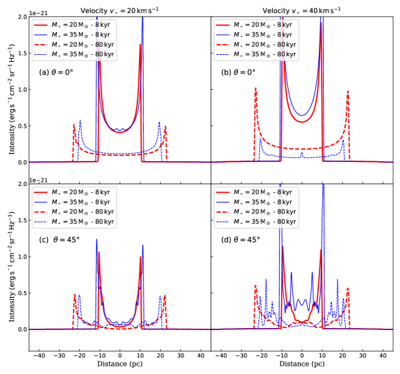
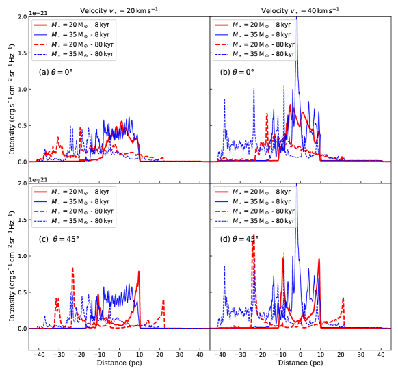
Figure 8: Horizontal (top) and vertical (bottom) cross-sections taken through non-thermal $1.4\,\rm GHz$ synchrotron emission maps of the supernova remnants.

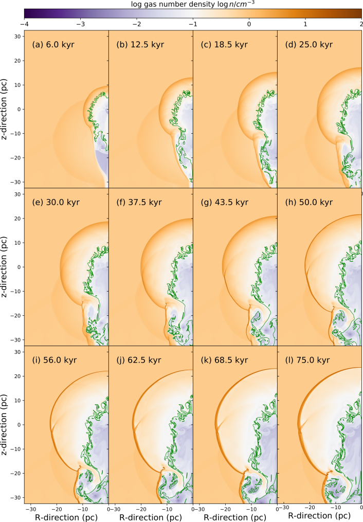
Figure 9: Time sequence evolution of the number density fields in the model corresponding to the most common supernova remnant, i.e. generated by a $20\,\rm M_{\odot}$ moving with velocity $v_{\star}=20\,\rm km\,\rm s^{-1}$. The remnant morphology evolves from bilateral to Cygnus Loop. The green contour mark the parts of the supernova remnants with a $50\%$ contribution of ejecta.

4 Discussion

This section proposes a comparison of the results with real, available observations. We particularly concentrate our analysis on bilateral and Cygnus-loop-like supernova remnants.

4.1 Limitations of the model

As in the previous papers of this series (Meyer et al., 2023), the present 2.5-dimensional magnetohydrodynamic simulations would benefit from a full three-dimensional treatment of the wind-ISM interactions and that of the ejecta-bubble calculation. Such simulations will add realisticness to the solution to our problem, especially concerning the stability of the pre-supernova magnetised circumstellar medium and fix the artificial ring-like artefacts arising from mapping 2.5-dimensional models into a 3-dimensional shape. It is not the maximum synchrotron surface brightness which would change, but rather the west-east symmetry concerning the $R=0$ direction that will disappear, as well as the series of horizontal bright lines ($\theta_{\rm obs}=0^{\circ}$) and ring-like ($\theta_{\rm obs}>0^{\circ}$) filaments located inside of the supernova remnant image, respectively. Those arcs will appear more ragged and clumpy while displaying more random distribution throughout the remnant’s interior. An illustration of the effects of full 3-dimensional emission maps can be found within the example of the optical H$\alpha$ bow shock of runaway red supergiant stars in Meyer et al. (2014) and  Meyer et al. (2021a).

The microphysical processes included in the numerical models also leave room for improvement, e.g. by including heat transfers or the ionisation of the supernova progenitor of the material of its circumstellar medium. The multi-phased character of the Galactic plane of the Milky Way is also an ingredient in our numerical model, which would benefit from future improvements. Particularly, initiating the wind-ISM models in a medium including turbulence, granularity provided by colder clumps and hotter cavities could potentially affect the supernova blastwave’s propagation and modify the current results. These issues will be considered in follow-up works. Last, the presence of a pulsar wind nebula could further modify the results (Blondin et al., 2001; Temim et al., 2015, 2017, 2022).

4.2 A time-sequence evolution?

This work covers the parameter space of the most common runaway massive supernova progenitors to investigate their morphologies and non-thermal radio appearance. The models in our study reveal that most of them undergo the formation of a bilateral supernova remnant when their supernova blastwave propagates through the preshaped circumstellar medium. Indeed, all models but one, i.e. all remnants generated by a red supergiant progenitor ($M_{\star}\geq 20\,\rm M_{\odot}$) or by a Wolf-Rayet progenitor ($M_{\star}\geq 35\,\rm M_{\odot}$) that is a slow runaway ($v_{\star}\approx 20\,\rm km\,\rm s^{-1}$) induce a bilateral supernova remnant made of two arcs produced when the shock wave interacts with the walls of the low-density cavity left behind the progenitor when moving before the explosion, at least for the ISM densities we consider. Additionally, in the case of a red supergiant progenitor, the bilateral morphology always precedes that of a Cygnus-loop-like morphology. We propose that each Cygnus-loop supernova remnant first came through an earlier phase during which it harboured a bilateral morphology. However, a bilateral shape will mostly but not necessarily evolve.

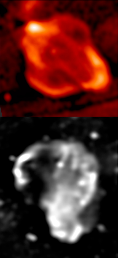
Figure 10: Radio images show a bilateral G309.2-00.6 (top panel, Ferrand & Safi-Harb, 2012) and the Cygnus Loop (bottom panel, Uyanıker et al., 2004) core-collapse supernova remnants. This study conjectures that bilateral remnants from massive stars are less common than those of Cygnus Loops but also that these shapes constitute a time-sequence of morphological evolution affecting the remnants of the most common runaway red supergiant progenitors.

In particular, we specifically conjecture that the Cygnus-loop nebula had once been in a bilateral shape. We also propose that the same must apply to Simeis 147, a supernova remnant of similar observed features: a bulb shape appears by the interaction between the blastwave and the circumstellar medium of its progenitor.

4.3 The occurrence of Cygnus-loop-like supernova remnants

The initial mass of massive stars as they form in the cold phase of the ISM of the Milky Way is determined by the so-called initial mass function, which, for high-mass stellar objects, reads,

$$dN(M_{\star})\propto M_{\star}^{-\zeta},$$ (49)

where $dN$ is the differential element of massive stars and $\zeta=2.3$ (see  Kroupa, 2001). Similarly, the space velocities of runaway massive stars as produced when a component of a massive binary system explodes is,

$$dN(v_{\star})\propto e^{-v_{\star}/v_{\rm max}},$$ (50)

with $v_{\rm max}=150\,\rm km\,\rm s^{-1}$ (see Bromley et al., 2009). The above mentioned distributions indicate that (i) most core-collapse supernova progenitors are massive stars in the lower region of the high mass spectrum (typically ending their lives as red supergiants and (ii) that runaway massive stars mostly move with small Mach numbers through the ISM (with typical supersonic velocities $v_{\star}\approx 20\,\rm km\,\rm s^{-1}$ in the plane of the Galaxy).

Our sample of supernova progenitors and space velocities (see Table 1) therefore covers the parameter space of the most common runaway progenitors and half of them, those involving a red supergiant progenitor, generate a Cygnus-loop morphology during the older times of their evolution. Since such progenitors are the most common runaway high-mass objects, we conjecture that a majority of supernova remnants of moving objects, i.e. that are either in the field or in the high latitudes of the Milky Way, display, or are in the process of forming a Cygnus-loop-like remnant. These objects are fainter than those of higher-mass progenitors, and, therefore, more difficult to observe. Consequently the supernova remnants to be discovered in the next decade by means of, e.g. the current James Webb Space Telescope (JWST) or the forthcoming Cherenkov Telescope Array (CTA) observatories, see  (Acharyya et al., 2023; Acero et al., 2023; Cherenkov Telescope Array Consortium et al., 2023), will, according to our results, reveal a majority of supernova remnants that are either in the bilateral or in the Cygnus-loop case, with a subset of the sooner gong to further evolve to the later.

4.4 Predictions for the most common supernova remnants

Fig. 9 displays the number density field in the simulation of the supernova remnant of initial mass $20\,\rm M_{\odot}$ moving with velocity $v_{\star}=20\,\rm km\,\rm s^{-1}$ through the ISM, for times spanning from $6\,\rm kyr$ to $75\,\rm kyr$. The green line marks the location of the discontinuity between supernova ejecta and the other kind of material (stellar wind and ISM). At early times the blastwave interacts strongly with the lateral region of the circumstellar medium, i.e. the wings of the stellar wind bow shock, which generates a bilateral shape, see Fig. 9a-d. The Cygnus Loop morphology begins to form at time $25\,\rm kyr$ after the onset of the explosion, with its characteristic shape made of two components: the overall mushroom of expanding supernova ejecta plus the tube of channelled material into the low-density cavity produced behind the progenitor as a result of its bluk motion through the ambient medium. The density of the shocked layer of ejecta, ISM and stellar wind that is swept-up by the forward shock of the supernova blastwave increases with time, compressing the local magnetic field better and enhancing the synchrtron emissivity (Fig. 9j-l). We conclude that this remnant spends about $18.5/80.0\approx 23\%$ of its early evolution time in the bilateral shape, while it harbors a Cygnus Loop morphology the rest of the time. Our results indicate therefore that the population of Cygnus Loop is $3$ times superior to that of bilateral remnants, at least for the conditions of ambient medium that we consider. However, the sooner are brighter than the later (Fig. 4), which is consistent with the more numerous detection of bilateral objects than Cygnus Loop amongst the known population of middle-aged to older core-collapse supernova remnants. Future high-resolution telescopes will help in building larger population statistics, which will better tests our prediction in the future.

How close are our predictions to real data? We plot in Fig. 10 the radio appearance of two core-collapse supernova remnants of bilateral and Cygnus Loop morphology, respectively. G309.2-00.6 is a bilateral remnant of age $\leq\,\rm 4\,\rm kyr$ and size $2$$-$$7\,\rm kpc$ that has a complex shape, superimposing large symmetric equatorial ears with two polar arcs, as seen in the top panel of Fig. 10. Literature on G309.2-00.6 is mostly observational. It soon revealed strong deviations of its morphology from the Sedov-Taylor solution, requiring the inclusion of circumstellar material pre-shaped by the progenitor’s stellar winds (Gvaramadze, 1999) and an explosive jet responsible for the second series of protuberances (Gaensler et al., 1998; Gaensler, 1999). Its size and age are consistent with our model while the model with $20\,\rm M_{\odot}$ and $v_{\star}=20\,\rm km\,\rm s^{-1}$, see Fig. 9a,b. Differences in the shape might be caused by the explosive jet that we do not model (Soker, 2023a) and/or by a different viewing angle of the supernova remnant. The Cygnus Loop is a peculiar supernova remnant that has been more studied, both by means of observations and with numerical models, than G309.2-00.6. Initially interpreted as a champagne outflow produced by a supernova explosion located at the edge of a molecular cloud (Aschenbach & Leahy, 1999), the Cygnus Loop nebula might be the outflow of a blast wave from a stellar wind bow shock (Meyer et al., 2015; Fang et al., 2017). Its size is estimated to be about $37\,\rm pc$ and its age $\approx 20\,\rm kyr$, which is in accordance with our same numerical model, see Fig. 9c,d. Hence, both remnants of different typical morphologies can qualitatively be explained by our model with $20\,\rm M_{\odot}$ and $v_{\star}=20\,\rm km\,\rm s^{-1}$.

5 Conclusion

In this study, we investigate the differences between the non-thermal synchrotron emission of supernova remnants generated by moving massive stars. Our parameter space covers the most common of such core-collapse supernova progenitors, of zero-age main-sequence mass $M_{\star}=20$ and $M_{\star}=35\,\rm M_{\odot}$, ending their lives as a red supergiant or as a Wolf-Rayet star, and moving into the warm phase of the Galactic plane with bulk velocities $v_{\star}=20\,\rm km\,\rm s^{-1}$ and $v_{\star}=40\,\rm km\,\rm s^{-1}$, respectively. The evolution of the supernova remnants is followed from the onset of the explosion to older ages ($80\,\rm kyr$). The methodology consists of performing 2.5-dimensional magneto-hydrodynamics numerical simulations of supernova blastwaves released into the circumstellar medium shaped by the interaction of the stellar wind of these moving progenitors with the ambient medium, see Meyer et al. (2023). Synchrotron emission calculations complete the magnetohydrodynamical structure to generate radio maps with physical units, instead of the usual normalised maps presented in most papers, that we compare to observations.

We find that most supernova remnants generated by a runaway massive star should undergo a phase exhibiting a bilateral morphology but that only those either generated by a red supergiant or, to a lesser extent, produced by a slightly supersonically moving Wolf-Rayet evolving progenitor, further develop as a Cygnus-loop-like supernova remnant (Aschenbach & Leahy, 1999; Meyer et al., 2015; Fang et al., 2017). Our $1.4\,\rm GHz$ non-thermal emission maps (Velázquez et al., 2023; Villagran et al., 2024) indicate that supernova remnants reveal duller projected intensities as the blastwave propagates through the defunct stellar surroundings and the unperturbed ISM and the remnant become old. In all explored scenarios, supernova remnants generated by faster-moving stars are brighter than those induced by stars, which were moving slower before dying. Their Cygnus-loop appearances do not survive when the viewing angle between the observer and the place of the sky is important ($\theta_{\rm obs}=45^{\circ}$).

Our methodology permits to investigate the time-dependant evolution of supernova remnants’ brightness, and, in future studies, we will apply it in the context of (plerionic) supernova remnants of static massive stars (Meyer et al., 2022, 2024). Our work particularly proposes a non-thermal synchrotron bilateral to Cygnus-loop-like morphological time sequence evolution for the appearance of Galactic supernova remnants, and that it should affect most of the dead stellar surroundings in the field since red supergiant progenitors are more common than heavier exploding stars. This implies that among the many supernova remnants to be discovered in the future, e.g. by means of the forthcoming Cherenkov Telescope Array (CTA), observatory (Acharyya et al., 2023; Acero et al., 2023; Cherenkov Telescope Array Consortium et al., 2023), a significant fraction of them should be undergoing this bilateral-to-Cygnus-loop evolutionary sequence.