Counting statistics of ultra-broadband microwave photons

Abstract

We report measurements of counting statistics, average and variance, of microwave photons of ill-defined frequency: bichromatic photons, i.e. photons involving two well separated frequencies, and ”white”, broadband photons. Our setup allows for the detection of single photonic modes of arbitrary waveform over the 1-10 GHz frequency range. The photon statistics is obtained by on-the-fly numerical calculation from the measured time-dependent voltage. After validating our procedure with thermal and squeezed radiation of such photons, we relate the detected statistics to the squeezing spectrum of an ac+dc biased tunnel junction. We observe an optimal squeezing of $\sim 1.5\text{$\mathrm{dB}$}$ over a bandwidth $>1$ GHz, better than $1\text{$\mathrm{dB}$}$ over 3.5 GHz and still see squeezing over a bandwidth of $\sim 6$ GHz centered on 6 GHz. We also show how the waveform of a bichromatic photon can be optimized for maximum squeezing.

Quantum correlations in the electromagnetic field is a key resource in the development of quantum technologies. Entangled light can substantially improve the signal to noise ratio in imaging [1, 2], gravitational wave detection [3] and is currently used to accelerate dark matter research [4].

To achieve high entanglement generation rate in the microwave domain, a great effort has been put into adapting travelling wave parametric amplifiers (TWPA) [5, 6, 7] to produce broadband squeezed states. Widening the band over which squeezing occurs increases the number of useful entangled pairs in the signal. Indeed, TWPAs are outperforming Josephson parametric amplifiers (JPAs) by their squeezing bandwidth, from 0.7 $\mathrm{GHz}$[8, 9] to 4$\mathrm{GHz}$[7], while also promising a large amount of squeezing. While TWPAs are a fascinating and promising technology for the generation of large bandwidth quantum states, they are complex to design and very difficult to fabricate.

Developing broadband sources also requires developing the theoretical and experimental tools to analyse their output field. A usual characterization consists of detecting the quadratures of the field at pairs of frequencies $F-\Delta$ and $F+\Delta$ symmetrically situated around $F$. Depending on the mechanism used to generate photon pairs, the central frequency $F$ could either be half of the pump frequency ($F=f_{p}/2$ for three wave mixing) or the pump frequency ($F=f_{p}$ for four wave mixing). The so-called squeezing spectrum, which measures the amount of squeezing vs. $\Delta$ is obtained by correlating the quadratures of the two frequencies. Such a detection suffers from its phase sensitivity: if the signal’s phase at frequency $F-\Delta$ rotates, the correlation with its mate at frequency $F+\Delta$ decays even though photon pairs have been generated. This way of detecting squeezing may be relevant for certain applications, but one may want to know whether there are pairs in the signal irrespective of their absolute phase with respect to the pump. After all, the phase rotation at each frequency could be in principle compensated. Moreover, the fact that TWPAs are broadband sources is somehow lost in the analysis: correlations could occur not only between pairs of frequencies that are symmetric with respect to $F$, there could be correlations between other frequencies, or between more than two frequencies.

In this article we develop another way of analyzing broadband signals, by measuring the counting statistics of single photonic modes that are not monochromatic but broadband, i.e. with no well-defined frequency. We achieve this goal by numerical treatment of the measured time-dependent voltage, following [10]. We focus on two photonic modes: i) bichromatic photons, i.e. photons of two simultaneous frequencies, and ii) ”white” photons, i.e. single modes having a broad frequency content, up to 1 to 10 GHz. Analyzing the signal using bichromatic mode provides the squeezing spectrum without the phase rotation problem. Analyzing it in terms of wideband modes allows to look for broader squeezing and to probe for coherence in the mechanism generating the analyzed signal.

We have applied our technique to the ultra-broadband electronic noise generated by a tunnel junction properly dc+ac biased. Without ac bias, such a junction emits almost thermal radiation with the number of emitted photons being tunable by the dc bias. This offers us a way to test our setup. In the presence of a dc+ac bias, the junction emits squeezed radiation [11, 12]. Even though this device is extremely easy to fabricate, it provides a quantum radiation of bandwidth in principle only limited by the RC time of the junction, here $>15$ GHz.

I Principle of the measurement

We consider experiments in the microwave domain where a source placed at ultra-low temperature generates an electromagnetic radiation that propagates along a coaxial cable and is detected by a matched amplifier. In this setup the measured quantity is the time-dependent voltage amplitude of that wave, represented by the operator $\hat{v}$, superimposed on the noise of the amplification scheme. After further amplification, the signal is digitized at high speed and all the relevant quantities are computed from the digitized signal.

I.1 First quantization: definition of modes

In order to compute the photon statistics of the signal, one has to define which photons to count. In [10] the chosen basis was that of photons localized in time, at the extreme opposite of the usual first quantization in the frequency domain. In a real experiment, one has to mitigate both approaches by considering wavelets of finite time and frequency spread. We note $\beta(t)$ such wavelets in time domain and $\beta(f)$ in frequency domain; they correspond to the current mode of interest. Since $\beta(t)$ is real, $\beta(-f)=\beta^{*}(f)$. We start by considering two such wavelets $\beta_{1,2}$ centered around frequencies $f_{1,2}$ that are well separated so that $\beta_{1}$ and $\beta_{2}$ do not overlap. Typically, the width of $\beta_{1,2}(f)$ is $\sim 200$MHz whereas $f_{2}-f_{1}$ varies between 1 and 10 GHz. We define the annihilation operators $a_{1,2}$ of photons in the modes $\beta_{1,2}$ by:

$$\hat{a}_{1,2}=\int_{0}^{+\infty}\beta_{1,2}(f)\hat{a}(f)df\;\;\;,$$ (1)

where $\hat{a}(f)$ is the usual annihilation operator for a photon at frequency $f$. Since the wavelets $\beta_{1,2}(f)$ are narrow in frequency domain, one can simply think of the operators $\hat{a}_{1,2}$ as annihilating photons of frequency $f_{1,2}$ which would correspond to the limit $\beta_{1,2}(f)=\delta(f-f_{1,2})$. The $\beta$ functions are normalized according to:

$$\int|\beta(f)|^{2}\differential{f}=1\;\;\;.$$ (2)

since they correspond to single photonic modes (see e.g. [13]). From this we define the annihilation operator for a bichromatic photon,

$$\hat{b}=\frac{\hat{a}_{1}+\hat{a}_{2}}{\sqrt{2}}\;\;\;.$$ (3)

This operator annihilates a photon of mode $\beta=(\beta_{1}+\beta_{2})/\sqrt{2}$. Here the plus sign between the monochromatic annihilation operators $\hat{a}_{1,2}$ is arbitrary. One may consider a minus sign or any complex phase as well (we studied experimentally this for the photon statistics of squeezed radiation, see below). The photon number operator is defined by:

$$\hat{n}=\hat{b}^{{\dagger}}\hat{b}=\frac{\hat{n}_{1}+\hat{n}_{2}}{2}+\hat{\Delta}\;\;,\;\;\text{with }\hat{\Delta}=\frac{\hat{a}^{{\dagger}}_{1}\hat{a}_{2}+\hat{a}^{{\dagger}}_{2}\hat{a}_{1}}{2}\;.$$ (4)

The photocount distribution of bichromatic photons is obtained by calculating the moments of $\hat{n}$. $\hat{n}$ is distinct from the total photon number operator $\hat{N}=\hat{a}^{{\dagger}}_{1}\hat{a}_{1}+\hat{a}^{{\dagger}}_{2}\hat{a}_{2}$ (see e.g. Barnett and Radmore [13] chapter 3). The former is a measure of the photon number in a single particular mode of the field as the latter is summed over all modes. Here for example, we can complete the 2-frequency basis by introducing $\hat{c}=(\hat{a}_{1}-\hat{a}_{2})/\sqrt{2}$ such that $\hat{N}=\hat{b}^{{\dagger}}\hat{b}+\hat{c}^{\dagger}\hat{c}$, $[\hat{b}^{{\dagger}},\hat{b}]=1$ and $[\hat{b}^{{\dagger}},\hat{c}]=0$.

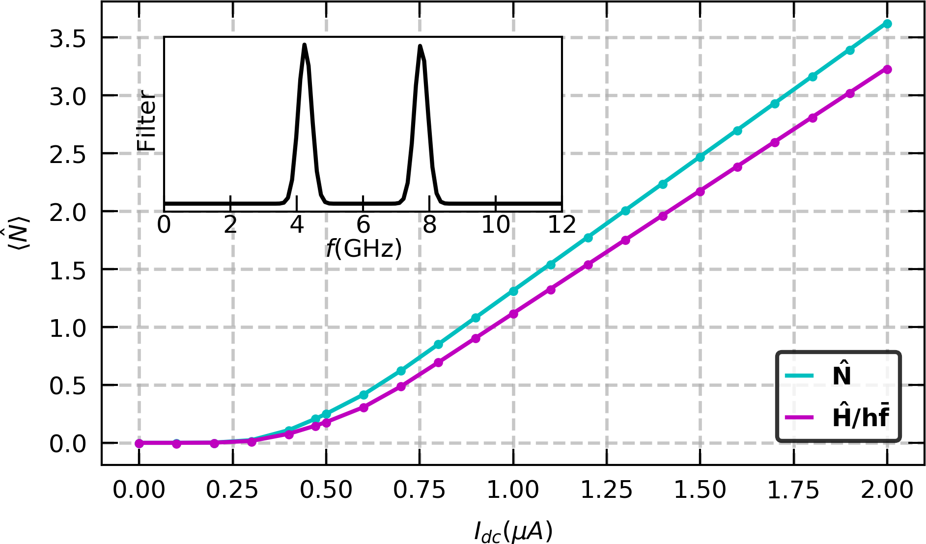
Figure 1: Total average photon number $\langle\hat{N}\rangle$ and total rescaled energy $\langle\hat{H}\rangle/h\bar{f}$ of bichromatic photons (at frequencies $f_{1}=4\text{$\mathrm{GHz}$}$ and $f_{2}=8\text{$\mathrm{GHz}$}$) generated by the dc biased tunnel junction as a function of the dc current in the junction. Using $\bar{f}=(f_{1}+f_{2})/2=6\text{$\mathrm{GHz}$}$ and $\hat{H}=\hat{v}^{2}/R$, with $R$ the sample’s resistance. There is no choice of $\bar{f}$ for which $\langle\hat{H}\rangle=\langle\hat{N}\rangle h\bar{f}$. Inset: The numerical filter used for this experiment.

Since we are dealing with broadband signals, the total number of photons $\hat{N}$ and the total energy $\hat{H}=\hbar\omega_{1}\hat{n}_{1}+\hbar\omega_{2}\hat{n}_{2}$ are not proportional. We illustrate this experimentally in Fig.1 where the total number of photons and the total energy, put in photon units, are plotted vs. the dc current in the sample: they do not coincide (see section II for the description of the measurement).

I.2 Quadrature Transform

The link between the measured time-dependent voltage $\hat{v}(t)$ and the photocount statistics is performed by defining the quadrature $\hat{x}(t)$ according to [10] :

$$\hat{x}(t)=\beta\operatorname{\circledast}k\operatorname{\circledast}\hat{v}\,(t)\;,$$ (5)

where $\operatorname{\circledast}$ is the convolution product and $k(t)=\sqrt{1/(Zh|t|)}$ with $Z$ the impedance of the detector, across which $\hat{v}$ is measured. $\hat{x}$ is the generalization to broadband signals of the usual quadrature of a signal at a given frequency $f$, i.e. its in-phase component. In frequency space, $\hat{x}(f)=\beta(f)k(f)\hat{v}(f)$ with

$$\hat{v}(f)=-i\sqrt{\frac{Zhf}{2}}\hat{a}(f)e^{-2i\pi ft}+\mathrm{H.c.}\;\;.$$ (6)

The kernel $k$ is chosen such that $\hat{x}(f)=[\hat{a}(f)+\hat{a}^{{\dagger}}(f)]/\sqrt{2}$ and $\beta$ defines the photonic mode, as discussed above.

I.3 Photocount statistics

From the computed time-dependent quadrature, we can deduce the photocount statistics. Herein we focus on the average photon number , $\expectationvalue{\hat{n}}$, and its variance , $\expectationvalue{\delta\hat{n}^{2}}$, with $\delta\hat{n}=\hat{n}-\expectationvalue{\hat{n}}$. The procedure is similar to what has been done in [14, 15], although differences arise from the large bandwidth involved here (see appendix B). We find:

$$\expectationvalue{\hat{n}} = \expectationvalue{\hat{x}^{2}}-\frac{1}{2}$$

$$\expectationvalue{\delta\hat{n}^{2}} = \frac{2}{3}\expectationvalue{\hat{x}^{4}}-\expectationvalue{\hat{x}^{2}}^{2}-\frac{1}{4}~{}~{}~{},~{}$$ (7)

where the average over $\hat{x}^{2}(t)$ and $\hat{x}^{4}(t)$ is experimentally taken over time. This is a generalization of the theoretical results of [14, 15] for any mode $\beta$ with certain restrictions concerning non-symmetric (n.s.) terms (i.e. terms that are non-symmetric with respect to conjugation, ex: $\hat{b}^{{\dagger}}\hat{b}^{3}$). These terms are set to be negligible either by construction (choosing $\beta(f)$ such that they are guaranteed to be 0) or by supposing that the light source guarantees $\expectationvalue{\text{n.s.}}=0$, which is the case for a tunnel junction.

II Methodology

II.1 Experimental setup

The experimental setup is depicted in Fig. 2. The source of the electromagnetic field is an Al / Al oxyde / Al tunnel junction of resistance $R=52.5\text{$\mathrm{\Omega}$}$ fabricated using standard photolithography and e-beam evaporation techniques. It is placed on the cold stage of a dilution refrigerator with a base temperature of $7$mK, with a strong rare earth magnet on the sample’s casing to keep the junction in its normal, non superconducting state.

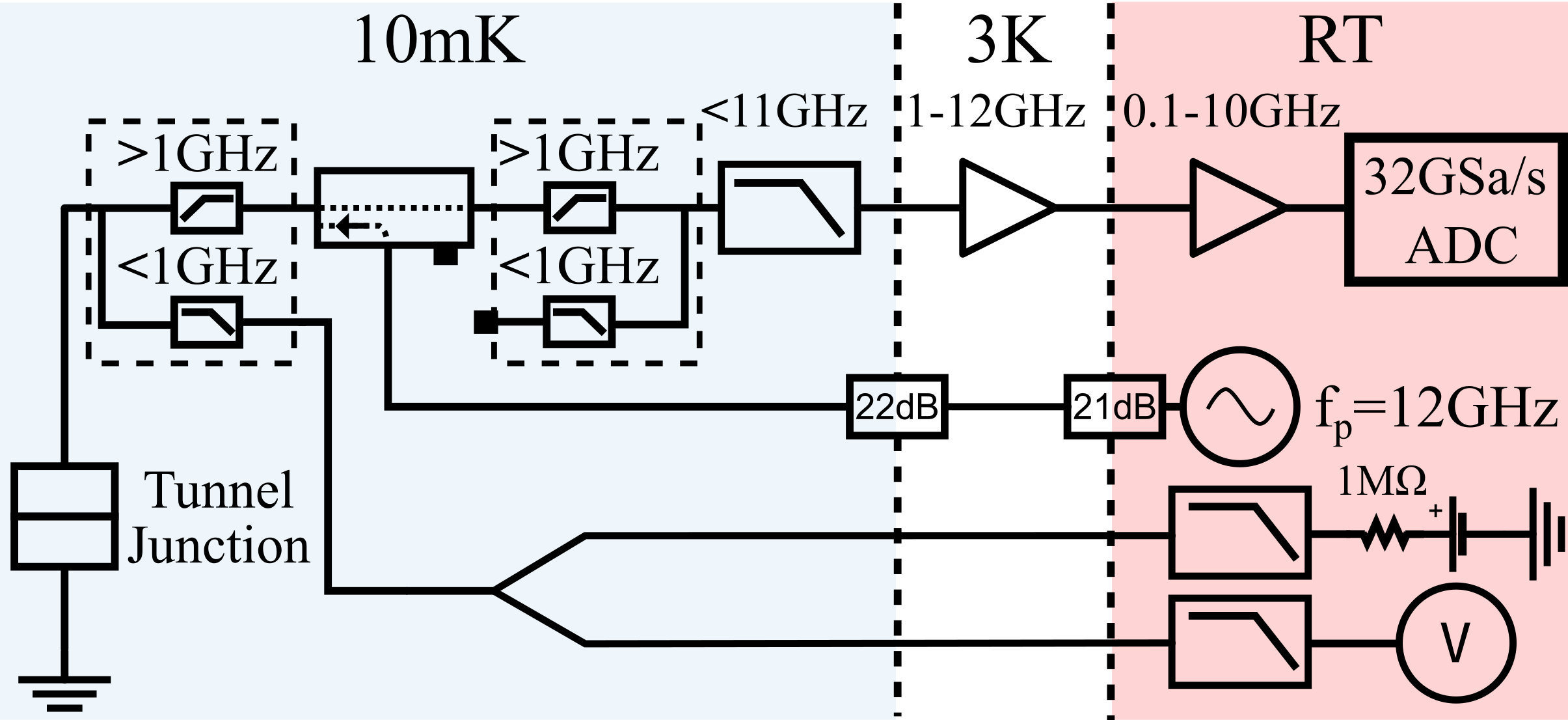
Figure 2: Experimental setup. The marker on the left represents the sample, a tunnel junction

The microwave radiation generated by the junction comes out of the high frequency ($>1\text{$\mathrm{GHz}$}$) branch of a diplexer pair, then is low-pass filtered $(<11\text{$\mathrm{GHz}$})$, goes through a cryogenic 1-12 GHz HEMT (LNF-LNC1-12A) amplifier followed by a room temperature amplifier and is finally digitized using a 10 bit, $32\text{GSa/sec}$ digitizer with $10\text{$\mathrm{GHz}$}$ analog bandwidth (Guzik ADP7104), resulting in a $1-10\text{$\mathrm{GHz}$}$ total analog bandwidth. The ac excitation reaches the sample through attenuated stainless steel coaxial cables followed by the $-20\text{$\mathrm{dB}$}$ port of a directional coupler. The excitation frequency $f_{p}=12\text{$\mathrm{GHz}$}$ is above the cutoff of the low-pass filter inserted in the detection line (-17.5 dB insertion loss at 12$\mathrm{GHz}$), so its reflection on the junction does not affect the measurement. The dc ports are low-pass filtered ($<6\text{$\mathrm{Hz}$}$) at room temperature before reaching the sample through Thermocoax cables ($<1\text{$\mathrm{MHz}$}$) all the way between room temperature and the $7\text{$\mathrm{mK}$}$ stage.

Achieving very low temperature without circulators.

Special care was crucial to reach an extremely low electron temperature $T_{\text{e}}<20\text{$\mathrm{mK}$}$. A first diplexer in front of the amplifier removes the low frequency noise (0-1 GHz) generated by the amplifier. A second diplexer connected to the sample plays the role of a bias tee without adding noise. Caution has been taken to avoid ground loops, in particular those involving the cryogenic amplifier’s power supply and the communication channels (USB, etc.).

Calibration

The power gain and electronic temperature $T_{\text{e}}$ are continuously measured and fitted from the full spectrum of current auto-correlations, as in [16]. The gain, used in the kernel for numerical deconvolutions (see Eq.(8)), is regularly updated. The average electronic temperature is $T_{e}\simeq 17\text{$\mathrm{mK}$}$ (see Appendix C), with minor fluctuations ($\sim 0.7$ mK) between experiments. Fluctuations in the noise temperature of the amplification chain are canceled out by alternating experimental conditions with references ($I_{\text{dc}}=0$,$I_{\text{ac}}=0$).

Finally, the attenuation along the ac port at $12\text{$\mathrm{GHz}$}$ ($\sim-79\text{$\mathrm{dB}$}$) is estimated by fitting the photo-excited auto-correlation, [16].

Nonlinearities.

The statistics of the voltage fluctuations generated by the sample are separated from that coming from the measurement setup by exploiting the linearity of cumulants for statistically independent variables, $\expectationvalue{\!\!\expectationvalue{\left(X+Y\right)^{k}}\!\!}=\expectationvalue{\!\!\expectationvalue{X^{k}}\!\!}+\expectationvalue{\!\!\expectationvalue{Y^{k}}\!\!}$ [14, 15, 16, 17]. This holds true only if the amplification chain is linear enough, as nonlinearities introduce artificial correlations between the noise of the sample and that of its detection. This effect worsens the higher the statistics and it is much preferable to minimize nonlinearities before acquisition than to rely on error-prone post-processing corrections. In our experiment, the main source of nonlinearity was traced down to the A/D converter of the digitizer and was mitigated by reducing by $6\text{$\mathrm{dB}$}$ the gain in the digitizer itself, i.e. only a small section (centered around 0 volts) of the 10 bits digital range is used. This sacrifice in dynamic range for linearity effectively resolved all nonlinearity-related issues in measurements, rendering further corrections unnecessary for the presented data.

II.2 Numerical methods

The $32\text{GSa/sec}$ voltage samples are numerically converted to photon quadrature using a homemade C++ implementation of the overlap-add method using FFTW for high performance hardware specific FFTs and parallelisation on a 36 cores (Dual Xeon E5-2697v4) server. Results shown herein require long averaging (for example, Fig. 4 took $\sim 2$ weeks of continuous averaging) and maximizing throughput helps both for faster experimental iterations and easier compensation for fluctuations in the setup properties (noise temperature fluctuation of the cryogenic amplifier, electrical noise from the power lines, etc.). The numerical convolutions with kernels of 257 points (number of time bins in $k\operatorname{\circledast}\beta(t)$) runs at about $2.0\text{GSa/sec}$ (1 sample is 10 bit) and a typical experimental loop (setting parameters, aquisition, transfert, numerical treatement) runs at an effective sample rate of $1.5\text{GSa/sec}$.

The digitized signal is deconvolved to remove the effect of the transfer function from the sample to the digitizer,

$$x(t) = \underbrace{k\operatorname{\circledast}\beta\operatorname{\circledast}|g|^{-1}}_{\text{numerical}}\operatorname{\circledast}\underbrace{g\operatorname{\circledast}[v_{s}(t)+v_{A}(t)]}_{\text{physical}}~{}~{}~{},~{}$$ (8)

where $k$ identifies the kernels transforming $\hat{v}\to\hat{x}$, $g$ is the voltage gain between the sample and the digitizer, $v_{s}$ is the sample’s voltage and $v_{A}$ is the voltage fluctuation added by the detection. No phase information is contained in our measurement of the power gain, hence we only deconvolve for the modulus of the transfer function, $|g(f)|$. This is enough as long as we consider only even order cumulants that only involve modulus squared of the voltage fluctuations, see below. A numerical kernel $k\operatorname{\circledast}\beta\operatorname{\circledast}|g|^{-1}$ is constructed for each mode during calibration and is reused during the experiment for each experimental condition. It is noteworthy that since $k\sim 1/\sqrt{|t|}$ contains poles both at $k(t=0)$ and $k(f=0)$ it needs to be regularized, see appendix A. As pointed out in [10], $k$ is not causal: $x(t)$ depends of future times. This is the price to pay to extract photon statistics from traces of the time-dependent voltage.

III Results

III.1 Bichromatic thermal radiation

We first test our experiment by measuring the photocount statistics of thermal radiation in a bichromatic single photonic mode, at 4GHz and 8GHz. The radiation comes from the current noise of the tunnel junction when dc biased. While the tunnel junction’s noise is not Gaussian, cumulants of order 3 and above are very small so the radiation generated by the junction is almost identical to the thermal one. Changing the dc bias on the junction increases the average photon number, like increasing the temperature does, but the link between the variance and average photon numbers remains the same: $\expectationvalue{\delta\hat{n}^{2}}=\expectationvalue{\hat{n}}(\expectationvalue{\hat{n}}+1)$.

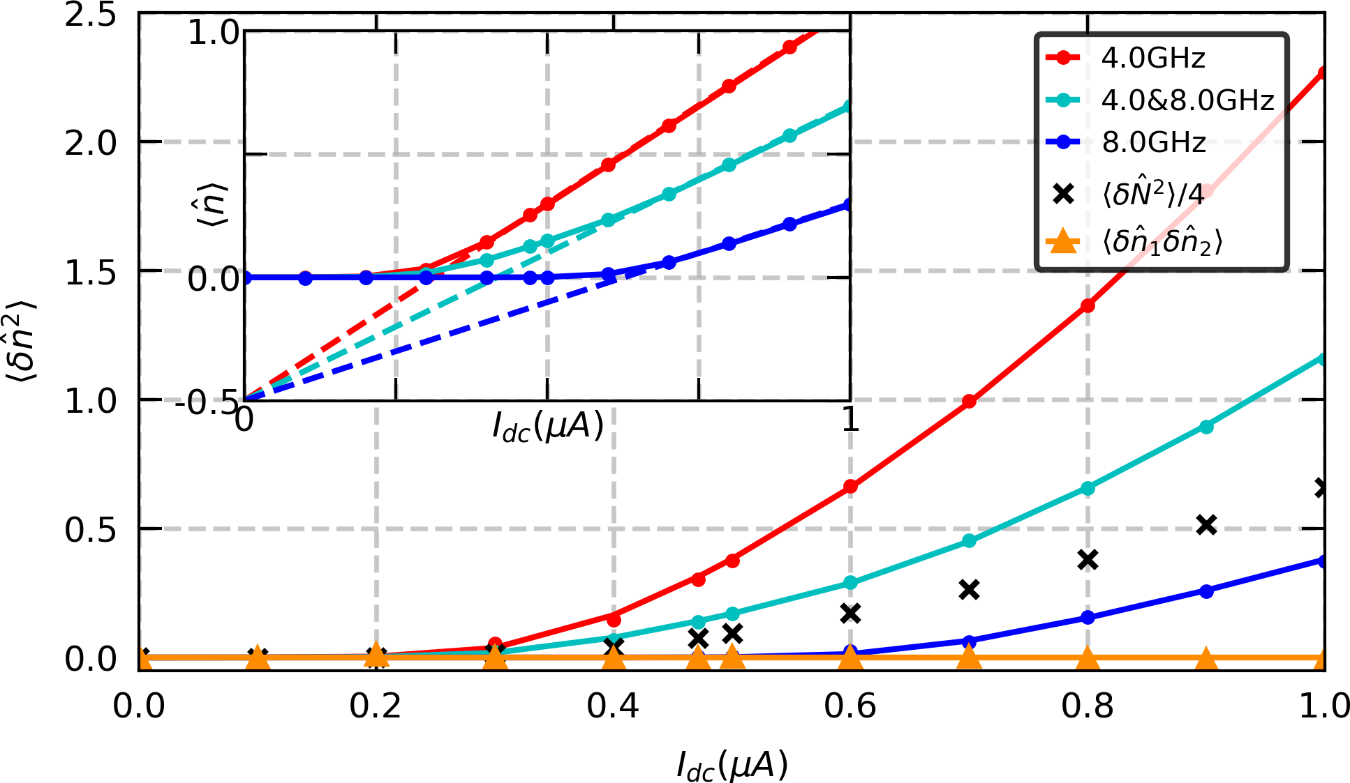
Figure 3: Variance of the photon number vs. dc current in the junction. Red (resp. blue) ’.’ markers correspond to monochrome modes at frequency $f_{1}=4\text{$\mathrm{GHz}$}$ (resp. $f_{2}=8\text{$\mathrm{GHz}$}$); cyan ’.’ markers correspond to the bichromatic mode at $4\&8\text{$\mathrm{GHz}$}$. black ’x’ markers correspond to $\langle\delta\hat{N}^{2}\rangle/4$ with $\hat{N}$ the total number of photons at frequencies $f_{1}$ and $f_{2}$; orange ’$\triangle$’ markers correspond to the correlation $\expectationvalue{\delta\hat{n}_{1}\delta\hat{n}_{2}}$. Solid lines are theoretical predictions : $\expectationvalue{\hat{n}}(\expectationvalue{\hat{n}}+1)$. Inset: average photon number vs. dc current in the junction.

This is true provided the statistics is performed on a single mode, irrespective of this mode being narrow-band or not. In Fig. 3 we show the measurements of $\expectationvalue{\hat{n}}$ (in inset) and $\expectationvalue{\delta\hat{n}^{2}}$ as a function of the dc bias current in the junction for the monochromatic modes $\hat{a}_{1}$ at frequency $f_{1}=4\text{$\mathrm{GHz}$}$ (red markers), $\hat{a}_{2}$ at $f_{2}=8\text{$\mathrm{GHz}$}$ (blue) as well as for the bichromatic mode $\hat{b}=(\hat{a}_{1}+\hat{a}_{2})/\sqrt{2}$ that encompasses both frequencies (cyan). The average photon number in the mode $\beta$ emitted by the junction is given by [18]:

$$\expectationvalue{\hat{n}}=2\int_{0}^{+\infty}|\beta(f)|^{2}\left(\frac{S_{2}(f)}{Rhf}-\frac{1}{2}\right)\differential{f}\;\;,$$ (9)

with $S_{2}(f)$ the current noise spectral density of the junction at frequency $f$. The factor two in front of the integral is inserted since $S_{2}(f)$ is usually defined for positive and negative frequencies. Solid lines for $\hat{n}_{1}$ and $\hat{n}_{2}$ in the inset of Fig.3 correspond to this formula. The average number of bichromatic photons is obviously given by $\expectationvalue{\hat{n}}=(\expectationvalue{\hat{n}_{1}}+\expectationvalue{\hat{n}_{2}})/2$ (cyan solid line). Solid lines in Fig. 3 correspond to $\expectationvalue{\hat{n}}(\expectationvalue{\hat{n}}+1)$. They closely follow our experimental data even in the bichromatic case, indicating that we are correctly counting bichromatic photons.

Let us now consider the operator $\hat{N}/2=(\hat{n}_{1}+\hat{n}_{2})/2$, the mean of photon number in modes 1 and 2. Its average value is the same as that of the single mode photon number $\hat{n}$. Its variance is given by:

$$\frac{1}{4}\expectationvalue{\delta\hat{N}^{2}}=\frac{1}{4}\left(\expectationvalue{\delta\hat{n}_{1}^{2}}+\expectationvalue{\delta\hat{n}_{2}^{2}}\right)+\frac{1}{2}\expectationvalue{\delta\hat{n}_{1}\delta\hat{n}_{2}}\;\;.$$ (10)

The last term, $\expectationvalue{\delta\hat{n}_{1}\delta\hat{n}_{2}}$, corresponds to correlations between photons emitted at different frequencies. There are no such correlations in thermal light, as confirmed experimentally, see the orange ’$\triangle$’ markers in Fig.3. Then Eq.(10) reduces to the fact that if two random variables are uncorrelated, their variances add. The measurement of $\expectationvalue{\delta\hat{N}^{2}}/4$ is plotted as black ’x’ markers in Fig. 3: it clearly differs from $\expectationvalue{\delta\hat{n}^{2}}$ and does not obey the photon statistics of thermal light. The difference between the two comes from the operator $\hat{\Delta}$ introduced in Eq.(4). $\hat{\Delta}(t)$ oscillates at frequency $f_{2}-f_{1}$ and is zero in average. Thus it does not contribute to the average photon number. However $\expectationvalue{\hat{\Delta}^{2}}\neq 0$ contributes to $\expectationvalue{\delta\hat{n}}^{2}$ to make it obey the statistics of thermal light. This term reflects the fact that electromagnetic field adds, $\hat{b}\propto\hat{a}_{1}+\hat{a}_{2}$, not the photon numbers, $\hat{n}\neq\hat{n}_{1}+\hat{n}_{2}$.

III.2 Bichromatic single mode squeezed radiation

In the presence of an ac excitation, the tunnel junction emits a two-mode squeezed radiation by noise modulation [12, 11]. We consider the case where a dc voltage $V_{\text{dc}}=hf_{p}/(2e)$ is superimposed on a sine wave at frequency $f_{p}=12\text{$\mathrm{GHz}$}$. In these conditions the junction emits pairs of photons at frequencies $f_{1}$ and $f_{2}$ such that $f_{1}+f_{2}=f_{p}$ (three wave mixing) where $f_{1}$ and $f_{2}$ can take any value between 0 and $f_{p}$[19]. Hereunder we consider the counting statistics of photons in the bichromatic mode $b$, as above. If the junction emitted pure squeezed vacuum, one would have the photocount variance given by $\expectationvalue{\delta\hat{n}^{2}}=2\expectationvalue{\hat{n}}(\expectationvalue{\hat{n}}+1)$, i.e. the double of that of thermal light[13]. The junction however does not emit only pairs of photons since $\expectationvalue{\hat{n}_{1}}\neq\expectationvalue{\hat{n}_{2}}$. The photocount variance has been measured in the limit $f_{1}\simeq f_{2}$ where the two sidebands were not resolved, i.e. in the limit of single-mode squeezing[15]. Here we extend these results to well separated frequencies $f_{1}=4$GHz and $f_{2}=8\text{$\mathrm{GHz}$}$. We characterize $\expectationvalue{\delta\hat{n}^{2}}$ by defining the Fano factor $\mathcal{F}=\expectationvalue{\delta\hat{n}^{2}}/\expectationvalue{\hat{n}}$. For thermal radiation, $\mathcal{F}=\expectationvalue{\hat{n}}+1$.

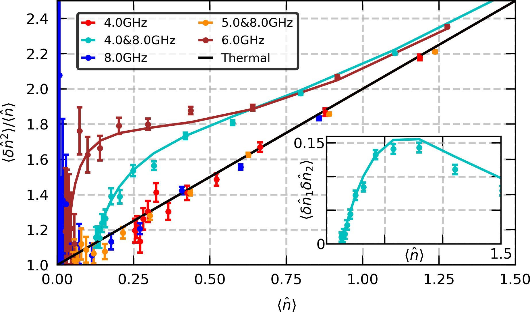
Figure 4: Fano factor as a function of the average photon number for different photonic modes. Markers are experimental data, solid lines theoretical predictions. Theory for monochromatic modes at 4GHz (red) and 6GHz (blue) as well as for the 5&8 GHz mode (orange) correspond to thermal light, i.e. $\mathcal{F}=(\expectationvalue{n}+1)$ (black line). The average photon number is varied by varying the amplitude of the ac drive at frequency $f_{p}=12$GHz with a constant dc bias $V_{\text{dc}}=hf_{p}/(2e)$. Inset: Correlation between photon numbers at 4 and 8 GHz vs. average bichromatic photon number.

We show in Fig. 4 Fano factors vs. $\expectationvalue{\hat{n}}$ for various amplitudes of the ac drive and various detection modes. If one detects only one frequency, such as 4GHz (red) or 8GHz (blue) which do not contain pairs of photons, one obtains thermal statistics (black), as well known for two-mode squeezed light[13]. A bichromatic mode made of two frequencies that do not add up to 12$\mathrm{GHz}$, such as 5GHz and 8GHz follow the same statistics (orange). The result for a monochromatic detection at 6GHz (brown) shows a clear deviation from $\expectationvalue{\hat{n}}+1$. It corresponds to the result reported in [15] with a lower electronic temperature. The cyan markers correspond to the case $f_{1}=4\text{$\mathrm{GHz}$}$, $f_{2}=8\text{$\mathrm{GHz}$}$: this bichromatic mode indeed bares the signature of the correlations existing between the electromagnetic fields at frequencies $f_{1}$ and $f_{2}$, characteristic of two-mode squeezed radiation. Theoretical expectation for squeezed condition, $6\text{$\mathrm{GHz}$}$ (brown) and $4\&8\text{$\mathrm{GHz}$}$ (cyan), are computed from the variance and fourth cumulant of current fluctuations as described in [19, 18].

The photocount variance can be rewritten as:

$$\expectationvalue{\delta\hat{n}^{2}}=\expectationvalue{\hat{n}}(\expectationvalue{\hat{n}}+1)+\expectationvalue{\delta\hat{n}_{1}\delta\hat{n}_{2}}\;\;.$$ (11)

As clear from this expression, the deviation from the statistics of thermal light uniquely comes from correlations between photons at frequencies $f_{1}$ and $f_{2}$. In the case of pure squeezed vacuum, only pairs are emitted so $\expectationvalue{\hat{n}}=\expectationvalue{\hat{n}_{1}}=\expectationvalue{\hat{n}_{2}}$ and $\expectationvalue{\delta\hat{n}_{1}\delta\hat{n}_{2}}=\expectationvalue{\delta\hat{n}_{1}^{2}}$, i.e. the Fano factor is doubled as compared to thermal light. In our experiment the junction emits pairs of photons [20], see the inset of Fig. 4, but not only.

The two measurements discussed until now were meant to demonstrate the ability of our experiment to measure the photocount statistics of broadband signals, in particular bichromatic ones with far apart frequencies. In the following we will apply it to explore some of the potential it offers to analyze more generally broadband radiation.

III.3 Squeezing spectrum

Analyzing two-mode squeezed radiation at far apart frequencies may be performed by detecting the variance of two quadratures (in-phase and out-of-phase) at each frequencies $f_{1}$ and $f_{2}$, i.e. $\hat{X}_{1,2}$ and $\hat{P}_{1,2}$, which are combined into $\hat{X}=(\hat{X}_{1}+\hat{X}_{2})/\sqrt{2}$ and $\hat{P}=(\hat{P}_{1}+\hat{P}_{2})/\sqrt{2}$. Correlations between quadratures at different frequencies, for example $\langle\hat{X}_{1}\hat{X}_{2}\rangle$ lead to the joint quadrature $\hat{X}$ having a variance below that of vacuum, i.e. $\langle\hat{X}^{2}\rangle<1/2$. This procedure usually requires having phase coherence between the detection at $f_{1}$ and $f_{2}$ as well as the excitation at $f_{p}$ that leads to the generation of squeezed vacuum by the sample, whatever it is [21]. In contrast, our technique does not require such stringent experimental constraints and is extremely frequency agile in the sense that analyzing another pair of frequencies only requires changing a single line of code. In fact, all the frequencies can be analyzed in parallel with a single acquisition. Our method however provides photocount statistics, not the variance of the quadratures. Below we show how these can be deduced from our measurements, which allows us to measure the squeezing spectrum of a broadband radiation [22, 23].

The quadratures at single frequencies $f_{1},f_{2}$ correspond to the operators $\hat{X}_{1,2}=(\hat{a}_{1,2}+\hat{a}^{{\dagger}}_{1,2})/\sqrt{2}$ and $\hat{P}_{1,2}=-i(\hat{a}_{1,2}-\hat{a}^{{\dagger}}_{1,2})/\sqrt{2}$. Considering again the bichromatic mode $\hat{b}=(\hat{a}_{1}+\hat{a}_{2})/\sqrt{2}$, the joint quadratures $\hat{X}$ and $\hat{P}$ can be expressed as a function of $\hat{b}$ and $\hat{b}^{{\dagger}}$ as : $\hat{X}=(\hat{X}_{1}+\hat{X}_{2})/\sqrt{2}=(\hat{b}+\hat{b}^{{\dagger}})/\sqrt{2}$ and $\hat{P}=(\hat{P}_{1}+\hat{P}_{2})/\sqrt{2}=-i(\hat{b}-\hat{b}^{{\dagger}})/\sqrt{2}$. This simply means that the two-mode squeezed state involving the modes $\hat{a}_{1}$ and $\hat{a}_{2}$ is in fact a single-mode squeezed state in terms of $\hat{b}$.

We now show how to deduce the variance of the two quadratures knowing the photon statistics for a mode $\hat{b}$ of any frequency content, not only bichromatic. Introducing the usual operator $\hat{m}=(\hat{b}^{2}+\hat{b}^{{\dagger}2})/2$, one has[23]:

$$\hat{n} = \frac{1}{2}(\hat{X}^{2}+\hat{P}^{2}-1)$$ (12)

$$\hat{m} = \frac{1}{2}(\hat{X}^{2}-\hat{P}^{2})\;\;.$$ (13)

$\hat{m}$ being sensitive to a global phase in $\hat{b}$, we choose it so $\expectationvalue{\hat{b}^{2}}$ is real and positive, i.e. so $\expectationvalue{\hat{m}}=\expectationvalue{\hat{b}^{2}}$. Supposing that $\hat{b}$ is Gaussian and applying Wick’s theorem to calculate $\expectationvalue{(\hat{b}^{{\dagger}}\hat{b})^{2}}$, we find:

$$\expectationvalue{\delta\hat{n}^{2}}=\expectationvalue{\hat{n}}(\expectationvalue{\hat{n}}+1)+\expectationvalue{\hat{m}}^{2}$$ (14)

which allows us to deduce $\expectationvalue{\hat{m}}$ from the photon statistics. $\expectationvalue{\hat{m}}$ measures the difference between the variance of $\hat{n}$ and its value for thermal radiation. In the case of the bichromatic mode, and using Eq.(11), one has: $\expectationvalue{\hat{m}}^{2}=\expectationvalue{\delta\hat{n}_{1}\delta\hat{n}_{2}}$, i.e. $\expectationvalue{\hat{m}}$ is also a measurement of the correlations between photons at frequencies $f_{1}$ and $f_{2}$.

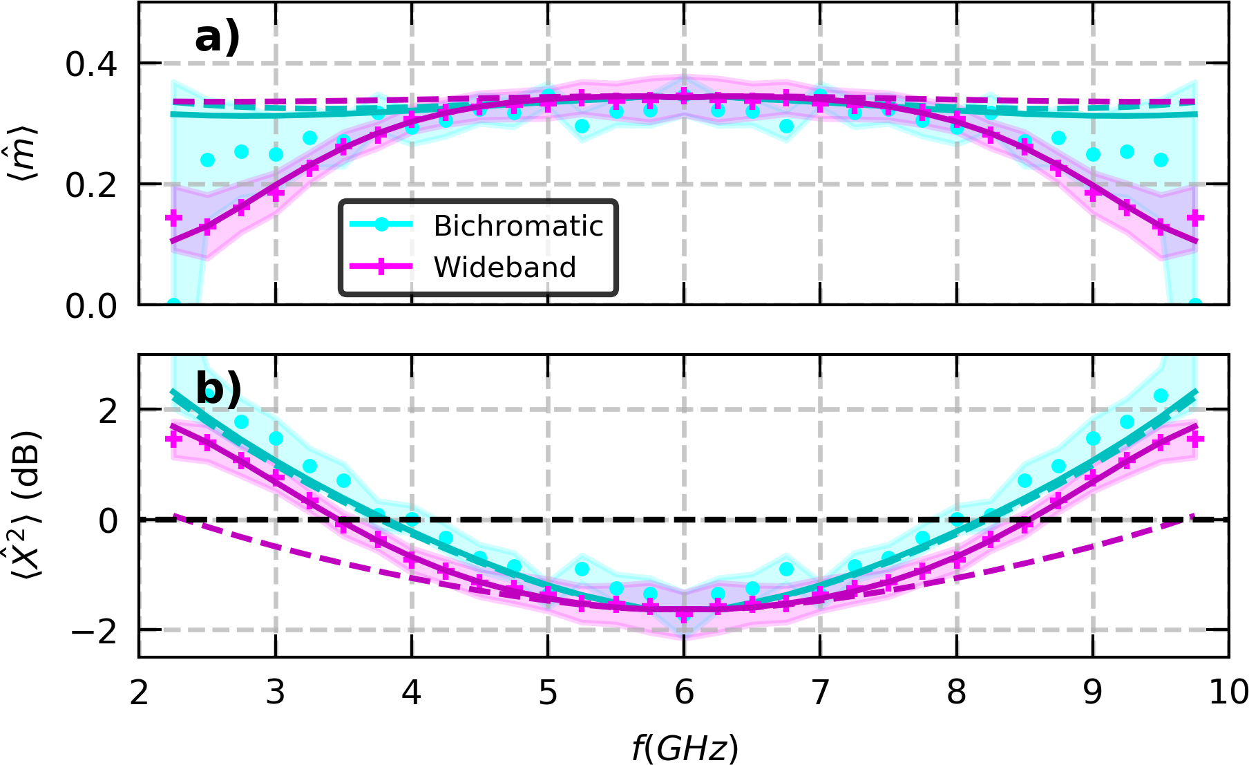
Figure 5: $\expectationvalue{\hat{m}}$ in linear scale (a) and variance of the quadrature $X$ in dB referred to vacuum (b) as a function of frequency $f$ for a tunnel junction excited at frequency $f_{p}=12$GHz with an RMS ac bias of $0.53\mu$A and $V_{\text{dc}}=hf_{p}/(2e)$. Cyan corresponds to bichromatic modes at frequencies $f$ and $f_{p}-f$ with a width of 200 $\mathrm{MHz}$. Pink corresponds to wideband photonic modes that extend from $f$ to $f_{p}-f$. Experimental uncertainty $(3\sigma)$ is represented as a shaded area around the average curve, ’.’ markers. The theory is presented using the same color with dashed lines for a dispersionless model and solid lines for a theory with a phase that increases quadratically with frequency. The black dashed horizontal line at 0dB (bottom graph) represents the vacuum level of fluctuations.

We now apply our technique to the broadband squeezed radiation generated by the tunnel junction. We show in Fig. 5 in cyan $\expectationvalue{\hat{m}}$ and the variance $\expectationvalue{\hat{X}^{2}}$ of bichromatic modes centered at frequencies $f$ and $f_{p}-f$ for $f$ varying between 2.25 and 9.75 GHz. It exhibits broadband two-mode squeezing from 4GHz to 8GHz. The squeezing we obtain is close to that of [5] with a much wider bandwidth, which is similar to that of the most advanced travelling wave parametric amplifiers (TWPAs)[7, 6]. While our tunnel junction provides less squeezing than the best TWPAs, it should be emphasized that its fabrication is by far less involved than that of a TWPA. Moreover, the bandwidth is only limited by that of the junction, which is greater than 15GHz and could probably be increased above 100GHz by working with more transparent junctions [24].

The case of ”white” photonic modes, which correspond to $\beta(f)$ uniform between $f$ and $f_{p}-f$, is displayed in pink in Fig. 5. These modes exhibit squeezing extending from 3.5 to 8.5 $\mathrm{GHz}$, starting at $\langle\hat{X}^{2}\rangle\sim-1.7\pm 0.4\text{$\mathrm{dB}$}$ for a narrow band detection around 6GHz, reaching $-1.5\pm 0.3\text{$\mathrm{dB}$}$ for the wideband mode 5-7GHz. $\langle\hat{X}^{2}\rangle<0\text{$\mathrm{dB}$}$ is observed for modes as wide as 3.5-8.5 GHz. The squeezing obtained with the wideband mode does not go lower than that obtained with bichromatic modes, but it stays at the minimum level on a wider frequency range. This probably stems from these modes containing pairs close to 6 $\mathrm{GHz}$, which are the most correlated.

Wideband modes have another remarkable property: since they involve a bandwidth much wider than the bichromatic modes, the signal to noise ratio of their measurement is much higher. For example, the bichromatic mode at 4 and 8 GHz has a bandwidth (the integrated area under $|\beta(f)|^{2}$) of 400 MHz while that of the wideband mode 4-8 GHz has a 10 times larger bandwidth, i.e. its measurement requires 10 times less time.

We show in Fig. 5 the theoretical expectations as dashed lines. The prediction for $\expectationvalue{\hat{m}}$ is remarkable, it is almost frequency independent over the whole frequency range: the junction is truly a broadband pair emitter. While theory and experiment match between 4 and 8 GHz, there is a discrepancy between both for too far apart frequencies, in particular for wideband modes. We think this is due to frequency dispersion in the detection. Phase rotation within the bandwidth of $\beta$ affects the measurement. For bichromatic modes, a significant phase rotation within 200MHz matters, but not between $f$ and $f_{p}-f$. Wideband modes are more sensitive to dispersion. Adding an artificial phase rotation that grows quadratically with frequency (a linear increase corresponds to a delay, which has no influence) leads to the solid lines in Fig. 5, which fits our data for a total rotation of $5\pi$ within 1-10GHz. Dashed and solid cyan lines are indistinguishable, in agreement with the fact that bichromatic modes very weakly sensitive to phase rotation. More experiments are needed, with a well calibrated phase response of the setup, to understand in depth the importance of dispersion in our measurement.

III.4 Choice of the mode $\beta$

Until now we have considered bichromatic modes with equal weights on the two frequencies. We now focus on the effect of the relative weights of the frequencies $f_{1}$ and $f_{2}$ by considering modes defined by:

$$\hat{d}(\lambda)=\sqrt{1-\lambda}\,\hat{a}_{1}+\sqrt{\lambda}\,\hat{a}_{2}\;\;\;,$$ (15)

which goes from $\hat{d}(\lambda=0)=\hat{a}_{1}$ to $\hat{d}(\lambda=1)=\hat{a}_{2}$ (adding a complex phase on either of the two terms does not influence the photon statistics). As above, we consider the effect of $\lambda$ on two quantities, $\expectationvalue{\hat{m}}$ and $\langle\hat{X}^{2}\rangle$. We fix the frequencies $f_{1}=4.25$ GHz and $f_{2}=7.75$ GHz and show in Fig. 6a $\expectationvalue{\hat{m}}$ vs. $\lambda$ for various ac currents in the junction. For $\lambda=0$ and $\lambda=1$, one has $\expectationvalue{\hat{m}}=0$ since there is no pair in the detection mode. The maximum is obtained for $\lambda=0.5$. Indeed:

$$\expectationvalue{\hat{m}} = 4\sqrt{\lambda(1-\lambda)}\mathrm{Re}\expectationvalue{\hat{a}_{1}\hat{a}_{2}}\;\;.$$ (16)

This is sound since a photon at frequency $f_{p}$ gives rise to a pair of photons, one at frequency $f_{1}$ and one at frequency $f_{2}$. The optimal detection is the one that respects this symmetry.

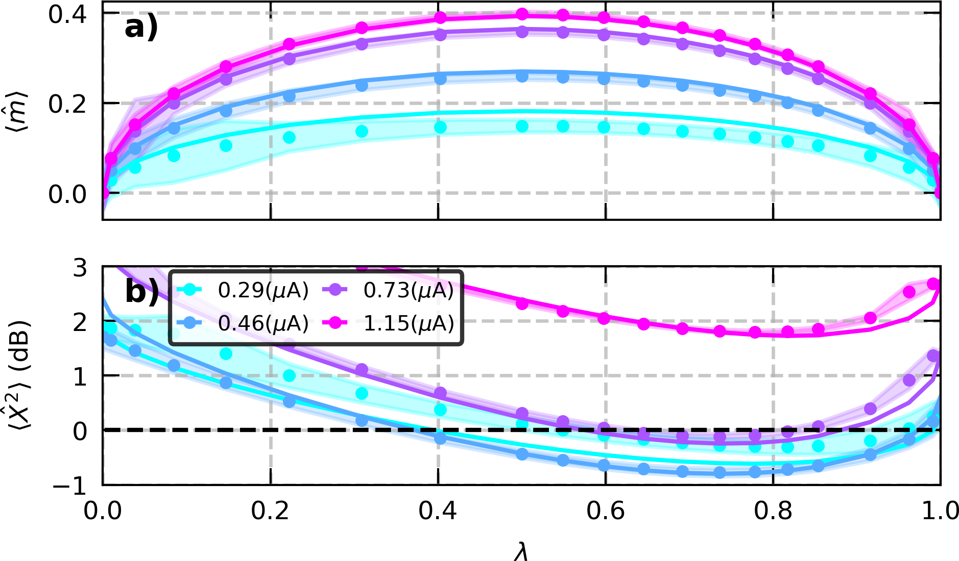
Figure 6: $\expectationvalue{\hat{m}}$ in linear scale (a) and variance of the quadrature $X$ in dB referred to vacuum (b) as a function of the parameter $\lambda$, see Eq.(15), with $f_{1}=4.25\text{$\mathrm{GHz}$}$ and $f_{2}=7.75\text{$\mathrm{GHz}$}$ and various ac excitations. Experimental uncertainty $(1\sigma)$ is represented as a shaded area around the average curve. Markers are experimental data and solid lines theory. The black dashed horizontal line represents the vacuum level of fluctuations.

We show in Fig.6b $\langle\hat{X}^{2}\rangle$ as a function of $\lambda$ for various ac currents in the junction. For $\lambda=0$ or $\lambda=1$ there is no squeezing as no photon pair is detected, thus $\langle\hat{X}^{2}\rangle>1/2$. Since $f_{2}>f_{1}$, $\expectationvalue{\hat{n}_{1}}>\expectationvalue{\hat{n}_{2}}$, thus $\langle\hat{X}^{2}\rangle$ is larger for $\lambda=0$ than for $\lambda=1$, as observed. In between there might be squeezing, as shown in Fig.5 which corresponds to $\lambda=0.5$. This value however does not correspond to the minimum, which is clearly closer to $1$ than to $0$. This comes from the fact that $\expectationvalue{\hat{n}_{1}}\neq\expectationvalue{\hat{n}_{2}}$: the junction emits not only pairs, it also emits single photons, and more at frequency $f_{1}$ than $f_{2}$. Thus the minimum of $\langle\hat{X}^{2}\rangle$ results from a compromise between having as much pairs as possible, i.e. $\lambda=0.5$ and having as little single photons as possible, i.e. $\lambda=1$. More precisely:

$$\langle\hat{X}^{2}\rangle = \frac{1}{2}+(1-\lambda)\expectationvalue{\hat{n}_{1}}+\lambda\expectationvalue{\hat{n}_{2}}$$ (17)

$$+ 4\sqrt{\lambda(1-\lambda)}\mathrm{Re}\expectationvalue{\hat{a}_{1}\hat{a}_{2}}\;\;.$$

We have discussed mode optimization only the case of bichromatic modes. For wideband modes, $\expectationvalue{\hat{m}}$ and $\langle\hat{X}^{2}\rangle$ depend on the shape of the mode $\beta(f)$, both its amplitude and phase. Finding the wideband mode that optimizes $\expectationvalue{\hat{m}}$ or $\langle\hat{X}^{2}\rangle$ is a captivating but daunting task that goes beyond the scope of this article. The same problem has been addressed with fermionic signals for which a procedure has been found [25]. Its extension to the case of a bosonic field that we are dealing with here would be of the utmost interest.

IV Conclusion

We have reported an experiment able to access the photon statistics of single modes with a frequency content that may span from 1 to 10 GHz. From this we showed how to deduce squeezing spectra and how to adjust the choice of bichromatic modes for optimal detection of squeezing. We have applied our setup to the broadband radiation emitted by a tunnel junction, which showed squeezing over a bandwidth from 4 to 8 GHz. Our technique can be applied to a large variety of wideband sources, from superconducting traveling wave parametric amplifiers (TWPAs) [26, 27, 23, 28, 29, 5, 7, 6] to maybe the radiation generated by quantum Hall conductors [30]. Other applications are those based on a dc voltage-biased Josephson junctions, for which there is no ac excitation, so no way to measure directly the quadratures [31, 32, 33, 34, 35]. Our experiment opens the possibility to deal not only with pairs of frequencies but with ultra-broadband signals. While in the parametric downconversion process, it is quite clear that one photon at frequency $f_{p}$ gives rise to a pair at frequencies symmetric around $f_{p}$, it is not clear at all that the mechanism of noise modulation involved in electronic noise is so simple. For example, does the junction emit randomly pairs of different frequencies, or broadband pulses which contain correlation among frequencies? In the latter case there could be correlations between different pairs. Our setup is the perfect tool to answer such questions, which could provide a new viewpoint on electronic quantum transport.

Appendix A Numerical convolution ($\hat{v}(t)\to\hat{x}(t)$)

In order to implement the convolution (5), we need a numerical representation for the kernel $k(t)$ that properly handles the pole at $t=0$. This is done by using the fact that the process of digitizing the signal with time step $\Delta t$ implies low-pass filtering at Nyquist frequency $f_{N}=1/(2\Delta t)$.

We use:

$$\frac{1}{\sqrt{|t|}} = \int_{0}^{+\infty}\frac{2\cos(2\pi ft)}{\sqrt{f}}\differential f$$

$$\approx \int_{0}^{f_{N}}\frac{2\cos(2\pi ft)}{\sqrt{f}}\differential f$$

$$= \frac{2\;\mathcal{C}(2\sqrt{f_{N}|t|})}{\sqrt{|t|}}~{}~{}~{},$$

where $\mathcal{C}$ is the Fresnel cosine integral, $\mathcal{C}=\int_{0}^{u}\cos(\frac{\pi x^{2}}{2})\differential x$. Similarly the Fresnel sine integral is $\mathcal{S}=\int_{0}^{u}\sin(\frac{\pi x^{2}}{2})\differential x$).

Applying the same process to the case $\Theta=0$ and $\Theta=\pi/2$ we find the discretized kernels to be:

$$k_{0}(n\Delta t) \approx 2\sqrt{\frac{2f_{N}}{Zh}}\begin{cases}0&\text{if }n=0\\ \textrm{sgn}(n)\frac{\;\mathcal{S}(\sqrt{2|n|})}{\sqrt{|n|}}&\text{if }n\neq 0\end{cases}$$

$$k_{\pi/2}(n\Delta t) \approx 2\sqrt{\frac{2f_{N}}{Zh}}\begin{cases}\sqrt{2}&\text{if }n=0\\ \frac{\mathcal{C}(\sqrt{2|n|})}{\sqrt{|n|}}&\text{if }n\neq 0\end{cases}$$

with $n$ integer. We chose $\Theta=0$, i.e. we have worked with the kernel $k=k_{0}$.

Appendix B Quadratures measurement

All even moments of the time dependent quadrature operator

$$\hat{x}_{\Theta}(t)=\frac{\hat{b}^{{\dagger}}(t)e^{i\Theta}+\hat{b}(t)e^{-i\Theta}}{\sqrt{2}}$$ (19)

can be split in two sums (we kept an arbitrary phase $\Theta$ for the sake of generality). The first sum contains the non-symmetric (n.s.) terms, i.e. with a different number of creation and annihilation operators in all orders; the second contains the completely symmetric (c.s.) terms, i.e. with the same number of creation and annihilation operators in all orders:

$$\hat{x}^{2k}_{\Theta}(t) = \frac{1}{2^{k}}\sum_{l=0}^{k-1}\sum_{\text{n.s.}}\bigg{[}\hat{b}(t)^{2k-l}\hat{b}^{{\dagger}l}(t)e^{i\Theta(-2k+2l)}+\text{h.c.}\bigg{]}$$ (20)

$$+ \frac{1}{2^{k}}\sum_{\text{c.s.}}\hat{b}^{k}(t)\hat{b}^{{\dagger}k}(t)\;\;.$$

The c.s. can be expressed in terms of photon number operator only [14, 15]:

$$\sum_{\text{c.s.}}=\sum_{i=0}^{k}\frac{(2k)!}{(i!)^{2}(k-i)!2^{k-i}}\prod_{j=0}^{i-1}\big{(}\hat{n}(t)-j\big{)}\;\;.$$ (21)

Since we are only interested in $k=1$ and $2$, we give their explicit form:

$$\hat{x}^{2}_{\Theta}(t) = \frac{\hat{b}^{2}(t)e^{-i2\Theta}+\text{h.c.}}{2}+\hat{n}(t)+\frac{1}{2}$$

$$\hat{x}^{4}_{\Theta}(t) = \frac{\hat{b}^{4}(t)e^{-i4\Theta}+\hat{b}^{3}(t)\hat{b}^{{\dagger}}(t)e^{-i2\Theta}+\text{h.c.}}{4}$$ (22)

$$+ \frac{3}{2}\hat{n}^{2}(t)+\frac{3}{2}\hat{n}(t)+\frac{3}{4}~{}~{}~{}.~{}$$

Averaging incoherently, i.e. without any synchronisation between the generation of the radiation by the ac drive in the sample and the clock of the digitization, simplifies the expressions of the c.s. and n.s. terms. If $\hat{b}$ describes a photon mode at frequency $f$, n.s. terms oscillate at frequencies $2(k-l)f$ and their time-average gives zero. This holds also for narrow-frequencies signals, so such terms were absent in [14, 15]. This is no longer true for $\hat{x}_{\Theta}^{4}(t)$ for wideband signals, as for example $\hat{b}^{3}(t)\hat{b}^{{\dagger}}(t)$ may contain a dc component provided the mode $\beta(f)$ is nonzero for some frequency $f$ as well as $3f$. In the particular case of bichromatic photons at frequencies $f_{1}$ and $f_{2}$, n.s. terms of $\hat{x}_{\Theta}^{4}(t)$ vanish upon time averaging except if $f_{2}=3f_{1}$. For general wideband signals, n.s. terms may contribute to the statistics of the quadratures. However for the shot noise we are considering here, n.s. terms are related to current correlators such as $\langle I(f_{1})I(f_{2})I(f_{3})(-f_{1}-f_{2}-f_{3})\rangle$ [36, 18] which are extremely small unless $f_{1}+f_{2}=f_{p}$ with $f_{p}$ the excitation frequency. In such a case $f_{1}+f_{2}+f_{3}>f_{p}$ is out of our detection bandwidth. Therefore n.s. terms never contribute here. In the absence of such terms, $\Theta$ becomes irrelevant, and we chose $\Theta=0$.

Appendix C Electronic Temperature

During the experiment the sample noise is continuously monitored in order to extract the power gain and noise temperature of the amplification line that slowly drift with time. We show in Fig. 7 the sample noise spectral density for several frequencies. For each frequency, by fitting the noise vs. bias we can precisely determine the electron temperature $T_{e}$. We plot in the inset of Fig. 7 the obtained $T_{e}$ vs. frequency. It is almost frequency independent, and corresponds to $T_{e}=17.4$mK.

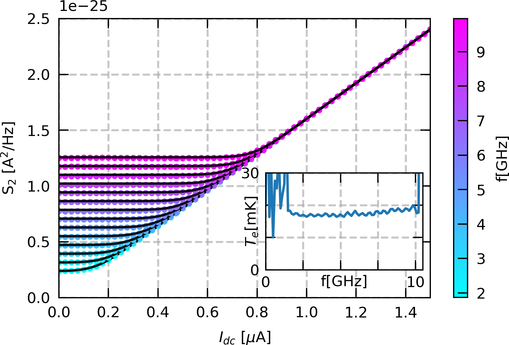
Figure 7: Noise spectral density $S_{2}(f)$, of our tunnel junction as a function of the dc bias current for frequencies between 2 and 10 GHz. Dots are measurements and lines are theoretical fits. Inset : The fitted electronic temperature as a function frequency.