Inferring Change Points in High-Dimensional Linear Regression via Approximate Message Passing

Abstract

We consider the problem of localizing change points in high-dimensional linear regression. We propose an Approximate Message Passing (AMP) algorithm for estimating both the signals and the change point locations. Assuming Gaussian covariates, we give an exact asymptotic characterization of its estimation performance in the limit where the number of samples grows proportionally to the signal dimension. Our algorithm can be tailored to exploit any prior information on the signal, noise, and change points. It also enables uncertainty quantification in the form of an efficiently computable approximate posterior distribution, whose asymptotic form we characterize exactly. We validate our theory via numerical experiments, and demonstrate the favorable performance of our estimators on both synthetic data and images.

1 Introduction

Heterogeneity is a common feature of large, high-dimensional datasets. When the data are ordered by time, a simple form of heterogeneity is a change in the data generating mechanism at certain unknown instants of time. If these ‘change points’ were known, or estimated accurately, the dataset could be partitioned into homogeneous subsets, each amenable to analysis via standard statistical techniques (Fryzlewicz, 2014). Models with change points have been studied in a variety of statistical contexts, such as the detection of changes in: signal means (Wang & Samworth, 2018; Wang et al., 2020; Liu et al., 2021); covariance structures (Cho & Fryzlewicz, 2015; Wang et al., 2021b); graphs (Londschien et al., 2023; Bhattacharjee et al., 2020; Fan & Guan, 2018); dynamic networks (Wang et al., 2021a); and functionals (Madrid Padilla et al., 2022). Change point models have found application in a range of fields including genomics (Braun et al., 2000), neuroscience (Aston & Kirch, 2012), and economics (Andreou & Ghysels, 2002).

In this paper, we consider high-dimensional linear regression with change points. We are given a sequence of data $(y_{i},\bm{X}_{i})\in{\mathbb{R}}\times{\mathbb{R}}^{p}$, for $i\in[n]$, from the model

$$y_{i}=(\bm{X}_{i})^{\top}{\bm{\beta}}^{(i)}+\varepsilon_{i},\quad i=1,\dots,n.$$ (1)

Here, ${\bm{\beta}}^{(i)}\in{\mathbb{R}}^{p}$ is the unknown regression vector for the $i$th sample, $\bm{X}_{i}\in{\mathbb{R}}^{p}$ is the (known) covariate vector, and $\varepsilon_{i}$ is additive noise. We denote the unknown change points, i.e., the sample indices where the regression vector changes, by $\eta_{1},\ldots,\eta_{L^{*}-1}$. Specifically, we have

$$1=\eta_{0}<\eta_{1}<\dots<\eta_{L^{*}}=n,$$

with ${\bm{\beta}}^{(i)}\neq{\bm{\beta}}^{(i-1)}$ if and only if $i\in\{\eta_{\ell}\}_{\ell=1}^{L^{*}-1}$. We note that $L^{*}$ is the number of distinct signals in the sequence $\{{\bm{\beta}}^{(i)}\}_{i=1}^{n}$, and $(L^{*}-1)$ is the number of change points. The number of change points is not known, but an upper bound $L$ on the value of $L^{*}$ is available. The goal is to estimate the change point locations as well as the $L^{*}$ signals. We would also like to quantify the uncertainty in these estimates, e.g., via confidence sets or a posterior distribution.

Linear regression with change points in the high-dimensional regime (where the dimension $p$ is comparable to, or exceeds, the number of samples $n$) has been studied in a number of recent works, e.g. (Lee et al., 2016; Leonardi & Bühlmann, 2016; Kaul et al., 2019; Rinaldo et al., 2021; Xu et al., 2022; Li et al., 2023; Bai & Safikhani, 2023). Most of these papers consider the setting where the signals are sparse (the number of non-zero entries in ${\bm{\beta}}^{(i)}\in{\mathbb{R}}^{p}$ is $o(p)$), and analyze procedures that combine the LASSO estimator (or a variant) with a partitioning technique, e.g., dynamic programming. The recent work of Gao & Wang (2022) assumes sparsity on the difference between signals across a change point, and Cho et al. (2024) consider general non-sparse signals. Although existing procedures for high-dimensional change point regression incorporate sparsity-based constraints, they cannot be easily adapted to take advantage of other kinds of signal priors. Moreover, they are not well-equipped to exploit prior information on the change point locations. Bayesian approaches to change point detection have been studied in several works, e.g. (Fearnhead, 2006; Lungu et al., 2022), however they mainly focus on (low-dimensional) time-series.

Main contributions

We propose an Approximate Message Passing (AMP) algorithm for estimating the signals $\{{\bm{\beta}}^{(i)}\}_{i=1}^{n}$ and the change point locations $\{\eta_{\ell}\}_{\ell=1}^{L^{*}-1}$. Under the assumption that the covariates are i.i.d. Gaussian, we give an exact characterization of the performance of the algorithm in the limit as both the signal dimension $p$ and the number of samples $n$ grow, with $n/p$ converging to a constant $\delta$ (Theorem 3.1). The AMP algorithm is iterative, and defined via a pair of ‘denoising’ functions for each iteration. We show how these functions can be tailored to take advantage of any prior information on the signals and the change points (Proposition 3.2). We then show how the change points can be estimated using the iterates of the AMP algorithm, and how the uncertainty can be quantified via an approximate posterior distribution (Section 3.3). Our theory enables asymptotic guarantees on the accuracy of the change point estimator and on the posterior distribution (Propositions 3.3, 3.4). In Section 4, we present experiments on both synthetic data and images, demonstrating the superior performance of AMP compared to other state-of-the-art algorithms for linear regression with change points.

Although our results do not explicitly need assumptions on the separation between adjacent change points, they are most interesting when the separation is of order $n$, i.e., $\Delta:=\min_{\ell\in[L]}(\eta_{\ell}-\eta_{\ell-1})=O(n)$. This separation is natural in our regime, where the number of samples $n$ is proportional to $p$ and the number of degrees of freedom in the signals also grows linearly in $p$. Existing results on high-dimensional change point regression usually assume signals that are $s$-sparse, and demonstrate change point estimators that are consistent when $\Delta=\omega\big{(}s\log p/\kappa^{2}\big{)}$, where $\kappa$ is a constant determined by the separation between the signals (Rinaldo et al., 2021; Wang et al., 2021c; Li et al., 2023). In contrast, we do not assume signal sparsity that is sublinear in $n$, so the change point estimation error will not tend to zero unless $n/p\to\infty$. We therefore quantify the AMP performance via precise asymptotics for the estimation error and the approximate posterior distribution.

Approximate Message Passing

AMP, a family of iterative algorithms first proposed for linear regression (Kabashima, 2003; Donoho et al., 2009; Krzakala et al., 2012), has been applied to a variety of high-dimensional estimation problems including estimation in generalized linear models (Rangan, 2011; Schniter & Rangan, 2014; Maillard et al., 2020; Mondelli & Venkataramanan, 2021) and low-rank matrix estimation (Fletcher & Rangan, 2018; Lesieur et al., 2017; Montanari & Venkataramanan, 2021; Barbier et al., 2020). An attractive feature of AMP algorithms is that under suitable model assumptions, their performance in the high-dimensional limit can be characterized by a succinct deterministic recursion called state evolution. The state evolution characterization has been used to show that AMP achieves Bayes-optimal performance for some models (Deshpande & Montanari, 2014; Donoho et al., 2013; Barbier et al., 2019).

An important feature of our AMP algorithm, in contrast to the above works, is the use of non-separable denoising functions. (We say a function $g:{\mathbb{R}}^{m\times L}\to{\mathbb{R}}^{m\times L}$ is separable if it acts row-wise identically on the input matrix.) Even with simplifying assumptions on the signal and noise distributions, non-separable AMP denoisers are required to handle the temporal dependence caused by the change points, and allow for precise uncertainty quantification around possible change point locations. Our main state evolution result (Theorem 3.1) leverages recent results by Berthier et al. (2019) and Gerbelot & Berthier (2023) for AMP with non-separable denoisers. Non-separable denoisers for AMP have been been studied for linear and generalized linear models, to exploit the dependence within the signal (Som & Schniter, 2012; Metzler et al., 2016; Ma et al., 2019) or between the covariates (Zhang et al., 2023). Here non-separable denoisers are required to exploit the dependence in the observations, caused by the change points.

Although we assume i.i.d. Gaussian covariates, based on recent AMP universality results (Wang et al., 2022), we expect the results apply to a broad class of i.i.d. designs. An interesting direction for future work is to generalize our results to rotationally invariant designs, a much broader class for which AMP-like algorithms have been proposed for regression without change points (Ma & Ping, 2017; Rangan et al., 2019; Takeuchi, 2020; Pandit et al., 2020).

2 Preliminaries

Notation

We let $[n]=\{1,2,\dots,n\}$. We use boldface notation for matrices and vectors. For vectors $\bm{x},\bm{y}\in{\mathbb{R}}^{n}$, we write $\bm{x}\leq\bm{y}$ if $x_{i}\leq y_{i}$ for all $i\in[n]$, and let $[\bm{x},\bm{y}]:=\{\bm{v}\in{\mathbb{R}}^{n}:x_{i}\leq v_{i}\leq y_{i}\;\forall i\in[n]\}$. For a matrix $\bm{A}\in{\mathbb{R}}^{m\times L}$ and $i\in[m],j\in[L]$, we let $\bm{A}_{[i,:]}$ and $\bm{A}_{[:,j]}$ denote its $i$th row and $j$th column respectively. Similarly, for a vector ${\bm{\psi}}\in[L]^{n}$, we let $\bm{A}_{[:,{\bm{\psi}}]}\in{\mathbb{R}}^{m}$ denote the vector whose $i$-th entry is $\bm{A}_{i,\psi_{i}}$.

For two sequences (in $n$) of random variables $X_{n}$, $Y_{n}$, we write $X_{n}\stackrel{{\scriptstyle{\mathbb{P}}}}{{\simeq}}Y_{n}$ when their difference converges in probability to 0, i.e., $\lim_{n\to\infty}{\mathbb{P}}(|X_{n}-Y_{n}|>\epsilon)=0$ for any $\epsilon>0$. Denote the covariance matrix of random vector $\bm{Z}\in\mathbb{R}^{q}$ as ${\rm{{Cov}}}(\bm{Z})\in\mathbb{R}^{q\times q}$. We refer to all random elements, including vectors and matrices, as random variables. When referring to probability densities, we include probability mass functions, with integrals interpreted as sums when the distribution is discrete.

Model Assumptions

In model (1), we assume independent Gaussian covariate vectors $\bm{X}_{i}\mathbin{\overset{i.i.d}{\kern 0.0pt\sim}}{\sf N}(0,\bm{I}_{p}/n)$ for $i\in[n]$. We consider the high-dimensional regime where $n,p\to\infty$ and $\frac{n}{p}$ converges to a constant $\delta>0$. Following the change point literature, we assume the number of change points $(L^{*}-1)$ is fixed and does not scale with $n,p$.

Pseudo-Lipschitz Functions

Our results are stated in terms of uniformly pseudo-Lipschitz functions (Berthier et al., 2019). For $C>0$ and $r\in[1,\infty)$, let $PL_{n,m,q}(r,C)$ be the set of functions $\phi:{\mathbb{R}}^{n\times q}\to{\mathbb{R}}^{m\times q}$ such that $\frac{\|\phi(\bm{x})-\phi(\tilde{\bm{x}})\|_{F}}{\sqrt{m}}\leq C\left(1+\left(\frac{\|\bm{x}\|_{F}}{\sqrt{n}}\right)^{r-1}+\left(\frac{\|\tilde{\bm{x}}\|_{F}}{\sqrt{n}}\right)^{r-1}\right)\frac{\|\bm{x}-\tilde{\bm{x}}\|_{F}}{\sqrt{n}}$ for all $\bm{x},\tilde{\bm{x}}\in{\mathbb{R}}^{n\times q}$. Note that $\cup_{C>0}PL_{n,m,q}(r_{1},C)\subseteq\cup_{C>0}PL_{n,m,q}(r_{2},C)$ for any $1\leq r_{1}\leq r_{2}$. A function $\phi\in PL_{n,m,q}(r,C)$ is called pseudo-Lipschitz of order $r$. A family of pseudo-Lipschitz functions is said to be uniformly pseudo-Lipschitz if all functions of the family are pseudo-Lipschitz with the same order $r$ and the same constant $C$. For functions $f:{\mathbb{R}}^{n\times m}\times{\mathbb{R}}^{n\times M}\to{\mathbb{R}}$ of the form $f(\bm{a},\bm{b})=c$, we say $f$ is uniformly pseudo-Lipschitz with respect to $\bm{a}$ if the family $\{f_{n}(\cdot,\bm{b}):n\in{\mathbb{N}},\bm{b}\in{\mathbb{R}}^{n\times M}\}$ is uniformly pseudo-Lipschitz. For $\bm{x},\bm{y}\in{\mathbb{R}}^{n}$, the mean squared error $\phi(\bm{x},\bm{y})=\langle\bm{x}-\bm{y},\bm{x}-\bm{y}\rangle/n$ and the normalized squared correlation $\phi(\bm{x},\bm{y})=|\langle\bm{x},\bm{y}\rangle|/n$ are examples of uniformly pseudo-Lipschitz functions.

3 AMP Algorithm and Main Results

We stack the feature vectors, observations and noise elements, respectively, to form $\bm{X}=[\bm{X}_{1},\dots,\bm{X}_{n}]^{\top}\in{\mathbb{R}}^{n\times p}$, $\bm{y}:=[y_{1},\dots,y_{n}]\in\mathbb{R}^{n}$ and $\bm{\varepsilon}:=[\varepsilon_{1},\dots,\varepsilon_{n}]^{\top}\in{\mathbb{R}}^{n}$. Let ${\bm{\eta}}:=[\eta_{1},\dots,\eta_{L^{*}},\dots,\eta_{L}]$ be the vector containing the true change points, and $\bm{B}:=[{\bm{\beta}}^{(\eta_{1})},\dots,{\bm{\beta}}^{(\eta_{L^{*}})},\dots,{\bm{\beta}}^{(\eta_{L})}]\in{\mathbb{R}}^{p\times L}$ be the matrix containing the true signals. Since the algorithm assumes no knowledge of $L^{*}$, other than $L^{*}\leq L$, the columns $L^{*}+1,\ldots,L$ of ${\bm{B}}$ can all be taken to be zero. Similarly, $\eta_{L^{*}}=\eta_{L^{*}+1}=\dots=\eta_{L}=n$.

Recall that for $i\in[n]$, each observation $y_{i}$ is generated from model (1). Let ${\bm{\Psi}}\in[L]^{n}$ be the signal configuration vector, whose $i$-th entry stores the index of the signal underlying observation $y_{i}.$ That is, for $i\in[n]$ and $\ell\in[L]$, let $\Psi_{i}=\ell$ if and only if ${\bm{\beta}}^{(i)}$ equals the $\ell$th column of the signal matrix ${\bm{B}}$. We note that that there is a one-to-one correspondence between ${\bm{\Psi}}$ and the change point vector ${\bm{\eta}}$. We can then rewrite $\bm{y}$ in a more general form:

$$\bm{y}=(\bm{X}\bm{B})_{[:,{\bm{\Psi}}]}+\bm{\varepsilon}:=q(\bm{X}\bm{B},{\bm{\Psi}},\bm{\varepsilon})\in{\mathbb{R}}^{n},$$ (2)

where $q$ acts row-wise on matrix inputs. We note that the mixed linear regression model (Yi et al., 2014; Zhang et al., 2022; Tan & Venkataramanan, 2023) can also be written in the form in (2), with a crucial difference. In mixed regression, the components of ${\bm{\Psi}}$ are assumed to be drawn independently from some distribution on $[L]$, i.e., each $y_{i}$ is independently generated from one of the $L$ signals. In the change point setting, the entries of ${\bm{\Psi}}$ are dependent, since they change value only at entries $\eta_{1},\ldots,\eta_{(L^{*}-1)}$.

AMP Algorithm

We now describe the AMP algorithm for estimating $\bm{B}$ and ${\bm{\eta}}$. In each iteration $t\geq 1$, the algorithm produces an updated estimate of the signal matrix $\bm{B}$, which we call $\bm{B}^{t}$, and of the linearly transformed signal $\bm{\Theta}:=\bm{X}\bm{B}$, which we call $\bm{\Theta}^{t}$. These estimates have distributions that can be described by a deterministic low-dimensional matrix recursion called state evolution. In Section 3.3, we show how the estimate $\bm{\Theta}^{t}$ can be combined with $\bm{y}$ to infer ${\bm{\eta}}$ with precisely quantifiable error.

Starting with an initializer $\bm{B}^{0}\in{\mathbb{R}}^{p\times L}$ and defining $\hat{{\bm{R}}}^{-1}:={\bm{0}}_{n\times L},$ for $t\geq 0$ the algorithm computes:

$$\begin{split}&\bm{\Theta}^{t}=\bm{X}\hat{\bm{B}}^{t}-\hat{{\bm{R}}}^{t-1}(\bm{F}^{t})^{\top}\,,\;\;\;\hat{{\bm{R}}}^{t}=g^{t}\left(\bm{\Theta}^{t},\bm{y}\right)\,,\\ &\bm{B}^{t+1}=\bm{X}^{\top}\hat{{\bm{R}}}^{t}-\hat{\bm{B}}^{t}(\bm{C}^{t})^{\top}\,,\;\;\;\hat{\bm{B}}^{t}=f^{t}\left(\bm{B}^{t}\right),\,\\ \end{split}$$ (3)

where the denoising functions $g^{t}:\mathbb{R}^{n\times L}\times\mathbb{R}^{n}\to\mathbb{R}^{n\times L}$ and $f^{t}:\mathbb{R}^{p\times L}\to\mathbb{R}^{p\times L}$ are used to define the matrices $\bm{F}^{t}$, $\bm{C}^{t}$ as follows:

$$\bm{C}^{t} =\frac{1}{n}\sum_{i=1}^{n}\partial_{i}{g^{t}_{i}}\left(\bm{\Theta}^{t},\bm{y}\right)\,,\;\;\;\bm{F}^{t}=\frac{1}{n}\sum_{j=1}^{p}\textrm{d}_{j}{f_{j}^{t}}(\bm{B}^{t}).$$

Here $\partial_{i}{g^{t}_{i}}\left(\bm{\Theta},\bm{y}\right)$ is the $L\times L$ Jacobian of $g^{t}_{i}$ w.r.t. the $i$th row of $\bm{\Theta}$. Similarly, $\textrm{d}_{j}{f_{j}^{t}}(\bm{B}^{t})$ is the $L\times L$ Jacobian of $f_{j}^{t}$ with respect to the $j$-th row of its argument. The time complexity of each iteration in (LABEL:eq:amp) is $O(npL+r_{n})$, where $r_{n}$ is the time complexity of computing $f^{t},g^{t}$.

Crucially, the denoising functions $g^{t}$ and $f^{t}$ are not restricted to being separable. (Recall that a separable function acts row-wise identically on its input, i.e., $g:{\mathbb{R}}^{m\times L}\to{\mathbb{R}}^{m\times L}$ is separable if for all $\bm{U}\in{\mathbb{R}}^{m\times L}$ and $i\neq j$, we have $[g(\bm{U})]_{i}=g_{i}(\bm{U}_{i})=g_{j}(\bm{U}_{i})$.) Hence, in general, we have

$$g^{t}(\bm{\Theta},\bm{y})=\begin{bmatrix}g^{t}_{1}(\bm{\Theta},\bm{y})\\ \vdots\\ g^{t}_{n}(\bm{\Theta},\bm{y})\end{bmatrix},\quad f^{t}(\bm{B})=\begin{bmatrix}f_{1}^{t}(\bm{B})\\ \vdots\\ f_{n}^{t}(\bm{B})\end{bmatrix}.$$

Our non-separable approach is required to handle the temporal dependence created by the change points. For example, if there was one change point uniformly in distributed in $[n]$, then $g^{t}(\bm{\Theta},\bm{y})$ should take into account that $y_{i}$ is more likely to have come from the the first signal for $i$ close to $1$, and from the second signal for $i$ close to $n$. This is in contrast to existing AMP algorithms for mixed regression (Tan & Venkataramanan, 2023), where under standard model assumptions, it suffices to consider separable denoisers.

In Appendix G, we review the AMP algorithm and state evolution for the generalized linear model without change points, i.e., the model in (2) without the vector ${\bm{\Psi}}$. This is useful background for the state evolution characterization described below for the change point setting.

State Evolution

The memory terms $-\hat{{\bm{R}}}^{t-1}(\bm{F}^{t})^{\top}$ and $-\hat{\bm{B}}^{t}(\bm{C}^{t})^{\top}$ in our AMP algorithm (LABEL:eq:amp) debias the iterates $\bm{\Theta}^{t}$ and $\bm{B}^{t+1}$, and enable a succinct distributional characterization. In the high-dimensional limit as $n,p\to\infty$ (with $n/p\to\delta$), the empirical distributions of $\bm{\Theta}^{t}$ and $\bm{B}^{t+1}$ are quantified through the random variables $\bm{V}_{\bm{\Theta}}^{t}$ and $\bm{V}_{\bm{B}}^{t+1}$ respectively, where

$$\bm{V}_{\bm{\Theta}}^{t}:=\bm{Z}{\bm{\rho}}^{-1}{\bm{\nu}}^{t}_{\bm{\Theta}}+\bm{G}^{t}_{\bm{\Theta}}\,\in{\mathbb{R}}^{n\times L},$$ (4)

$$\bm{V}_{\bm{B}}^{t+1}:=\bm{B}{\bm{\nu}}^{t+1}_{\bm{B}}+\bm{G}^{t+1}_{\bm{B}}\,\in{\mathbb{R}}^{p\times L}.$$ (5)

The matrices ${\bm{\rho}},{\bm{\nu}}_{\bm{\Theta}}^{t},{\bm{\nu}}_{\bm{B}}^{t+1}\in{\mathbb{R}}^{L\times L}$ are deterministic and defined below. The random matrices $\bm{Z}$, ${\bm{G}}_{\bm{\Theta}}^{t}$, and ${\bm{G}}_{\bm{B}}^{t+1}$ are independent of $\bm{X}$, and have i.i.d. rows following a Gaussian distribution. Namely, for $i\in[n]$ we have $\bm{Z}_{i}\mathbin{\overset{i.i.d}{\kern 0.0pt\sim}}{\sf N}({\bm{0}},{\bm{\rho}})$. For $i\in[n],j\in[p]$ and $s,r\geq 0$, $(\bm{G}_{\bm{\Theta}}^{t})_{i}\mathbin{\overset{i.i.d}{\kern 0.0pt\sim}}{\sf N}({\bm{0}},{\bm{\kappa}}_{\bm{\Theta}}^{t,t})$ with ${\rm{{Cov}}}((\bm{G}_{\bm{\Theta}}^{r})_{i},(\bm{G}_{\bm{\Theta}}^{s})_{i})={\bm{\kappa}}_{\bm{\Theta}}^{r,s}$. Similarly, $(\bm{G}_{\bm{B}}^{t})_{j}\mathbin{\overset{i.i.d}{\kern 0.0pt\sim}}{\sf N}({\bm{0}},{\bm{\kappa}}_{\bm{B}}^{t,t})$ with ${\rm{{Cov}}}((\bm{G}_{\bm{B}}^{r})_{j},(\bm{G}_{\bm{B}}^{s})_{j})={\bm{\kappa}}_{\bm{B}}^{r,s}$. The $L\times L$ deterministic matrices ${\bm{\nu}}_{\bm{\Theta}}^{t},{\bm{\kappa}}_{\bm{\Theta}}^{r,s},{\bm{\nu}}_{\bm{B}}^{t},$ and ${\bm{\kappa}}_{\bm{B}}^{r,s}$ are defined below via the state evolution recursion.

Given the initializer $\bm{B}^{0}$ for our algorithm (LABEL:eq:amp), we initialize state evolution by setting ${\bm{\nu}}_{\bm{\Theta}}^{0}:={\bm{0}}$, and

$${\bm{\rho}}:=\frac{1}{\delta}\lim_{p\to\infty}\frac{1}{p}\bm{B}^{\top}\bm{B},\ {\bm{\kappa}}^{0,0}_{\bm{\Theta}}:=\frac{1}{\delta}\lim_{p\to\infty}\frac{1}{p}f^{0}({\bm{B}}^{0})^{\top}f^{0}({\bm{B}}^{0}).$$ (6)

Let $\tilde{g}_{i}^{t}(\bm{Z},\bm{V}_{\bm{\Theta}}^{t},{\bm{\Psi}},\bm{\varepsilon}):=g_{i}^{t}(\bm{V}_{\bm{\Theta}}^{t},q(\bm{Z},{\bm{\Psi}},\bm{\varepsilon}))$ and let $\partial_{1i}\tilde{g}_{i}^{t}$ be the partial derivative (Jacobian) w.r.t. the $i$th row of the first argument. Then, the state evolution matrices are defined recursively as follows:

$${{\bm{\nu}}}_{\bm{B}}^{t+1}:=\lim_{n\to\infty}\frac{1}{n}{\mathop{\mathbb{E}}}\left[\sum_{i=1}^{n}\partial_{1i}\tilde{g}_{i}^{t}(\bm{Z},\bm{V}_{\bm{\Theta}}^{t},{\bm{\Psi}},\bm{\varepsilon})\right],$$ (7)

$${\bm{\kappa}}_{\bm{B}}^{s+1,t+1}:=\lim_{n\to\infty}\frac{1}{n}{\mathop{\mathbb{E}}}\left[g^{s}\left(\bm{V}_{\bm{\Theta}}^{s},q(\bm{Z},{\bm{\Psi}},\bm{\varepsilon})\right)^{\top}\right.$$

$$\left.\hskip 92.47145ptg^{t}\left(\bm{V}_{\bm{\Theta}}^{t},q(\bm{Z},{\bm{\Psi}},\bm{\varepsilon})\right)\right],$$ (8)

$${\bm{\nu}}^{t+1}_{\bm{\Theta}}:=\frac{1}{\delta}\lim_{p\to\infty}\frac{1}{p}{\mathop{\mathbb{E}}}\left[\bm{B}^{\top}f^{t+1}(\bm{V}_{\bm{B}}^{t+1})\right],$$ (9)

$${\bm{\kappa}}_{\bm{\Theta}}^{s+1,t+1}:=\frac{1}{\delta}\lim_{p\to\infty}\frac{1}{p}{\mathop{\mathbb{E}}}\left[\left(f^{s+1}(\bm{V}_{\bm{B}}^{s+1})-\bm{B}{\bm{\rho}}^{-1}{\bm{\nu}}^{s+1}_{\bm{\Theta}}\right)^{\top}\right.$$

$$\left.\hskip 71.13188pt\left(f^{t+1}(\bm{V}_{\bm{B}}^{t+1})-\bm{B}{\bm{\rho}}^{-1}{\bm{\nu}}^{t+1}_{\bm{\Theta}}\right)\right].$$ (10)

The expectations above are taken with respect to $\bm{Z},\bm{V}_{\bm{\Theta}}^{t},\bm{V}_{\bm{\Theta}}^{s},\bm{V}_{\bm{B}}^{t+1}$ and $\bm{V}_{\bm{B}}^{s+1}$, and depend on $g^{t}$, $f^{t}$, $\bm{B}$, $\bm{\varepsilon}$, and ${\bm{\Psi}}$. The limits in (7)–(10) exist under suitable regularity conditions on $f_{t},g_{t}$, and on the limiting empirical distributions on $\bm{B},\bm{\varepsilon}$; see Appendix B. The dependence on $\bm{B}$, $\bm{\varepsilon}$ can also be removed under these conditions – this is discussed in the next subsection.

3.1 State Evolution Characterization of AMP Iterates

Recall that the matrices (6)–(10) are used to define the random variables $(\bm{V}_{\bm{\Theta}}^{t},\bm{V}_{\bm{B}}^{t+1})$ in (4),(5). Through these quantities, we now give a precise characterization of the AMP iterates $(\bm{\Theta}^{t}$, $\bm{B}^{t+1})$ in the high-dimensional limit. Theorem 3.1 below shows that any real-valued pseudo-Lipschitz function of $(\bm{\Theta}^{t}$, $\bm{B}^{t+1})$ converges in probability to its expectation under the limiting random variables $(\bm{V}_{\bm{\Theta}}^{t},\bm{V}_{\bm{B}}^{t+1})$. In addition to the model assumptions in Section 2, we make the following assumptions:

1. The following limits exist and are finite almost surely: $\lim_{p\to\infty}\|\bm{B}^{0}\|_{F}/\sqrt{p}$,   $\lim_{p\to\infty}\|\bm{B}^{\top}\bm{B}\|_{F}/p$, and $\lim_{n\to\infty}\|\bm{\varepsilon}\|_{2}/\sqrt{n}$.

2. For each $t\geq 0$, let $\tilde{g}^{t}:(\bm{u},\bm{z})\mapsto g^{t}(\bm{u},q(\bm{z},{\bm{\Psi}},\bm{\varepsilon}))$, where $(\bm{u},\bm{z})\in{\mathbb{R}}^{n\times L}\times{\mathbb{R}}^{n\times L}$. For each $i\in[n],j\in[p],$ the following functions are uniformly pseudo-Lipschitz: $f^{t},\tilde{g}^{t},\textrm{d}_{j}f_{j}^{t},\partial_{1i}\tilde{g}_{i}^{t}$.

3. For $s,t\geq 0$, the limits in (6)–(10) exist and are finite.

Assumptions $\ref{it:main-res-ass-1}-\ref{it:main-res-ass-3}$ are natural extensions of classical AMP results which assume separable signals and denoising functions. They are similar to those required by existing works on non-separable AMP (Berthier et al., 2019; Gerbelot & Berthier, 2023), and generalize these to the model (2), with a matrix signal ${\bm{B}}$ and an auxiliary vector ${\bm{\Psi}}\in[L]^{n}$.

Theorem 3.1.

Consider the AMP in (LABEL:eq:amp) for the Change Point Regression model in (2), with the model assumptions in Section 2 as well as $\ref{it:main-res-ass-1}-\ref{it:main-res-ass-3}$. Then for $t\geq 0$ and any sequence of uniformly pseudo-Lipschitz functions ${\bm{\varphi}}_{n}:{\mathbb{R}}^{n\times(L(t+1)+2)}\to{\mathbb{R}}$ and ${\bm{\varphi}}_{p}:{\mathbb{R}}^{p\times(L(t+2))}\to{\mathbb{R}}$,

$${\bm{\varphi}}_{n}(\bm{\Theta}^{0},\dots,\bm{\Theta}^{t},\bm{y},{\bm{\Psi}})$$

$$\stackrel{{\scriptstyle{\mathbb{P}}}}{{\simeq}}{\mathop{\mathbb{E}}}_{\bm{V}_{\bm{\Theta}}^{0},\dots,\bm{V}_{\bm{\Theta}}^{t},\bm{Z}}\{{\bm{\varphi}}_{n}(\bm{V}_{\bm{\Theta}}^{0},\dots,\bm{V}_{\bm{\Theta}}^{t},q(\bm{Z},{\bm{\Psi}},\bm{\varepsilon}),{\bm{\Psi}})\},$$ (11)

$${\bm{\varphi}}_{p}(\bm{B}^{1},\dots,\bm{B}^{t+1},\bm{B})$$

$$\hskip 28.45274pt\stackrel{{\scriptstyle{\mathbb{P}}}}{{\simeq}}{\mathop{\mathbb{E}}}_{\bm{V}_{\bm{B}}^{1},\dots,\bm{V}_{\bm{B}}^{t+1}}\{{\bm{\varphi}}_{p}(\bm{V}_{\bm{B}}^{1},\dots,\bm{V}_{\bm{B}}^{t+1},\bm{B})\},$$ (12)

as $n,p\to\infty$ with $n/p\to\delta$, where the random variables $\bm{Z},\bm{V}_{\bm{\Theta}}^{t}$ and $\bm{V}_{\bm{B}}^{t+1}$ are defined in (4), (5).

The proof of the theorem is given in Appendix A. It involves reducing the AMP in (LABEL:eq:amp) to a variant of the symmetric AMP iteration analyzed in (Gerbelot & Berthier, 2023, Lemma 14). We use a generalized version of their iteration which allows for the auxiliary quantities ${\bm{\Psi}},q(\bm{Z},{\bm{\Psi}},\bm{\varepsilon})$ to be included. Theorem 3.1 implies that any pseudo-Lipschitz function ${\bm{\varphi}}_{n}$ of $(\bm{\Theta}^{t},\bm{y})$ will converge in probability to a quantity involving an expectation over $(\bm{V}_{\bm{\Theta}}^{t},\bm{Z})$. An analogous statement holds for $(\bm{B}^{t+1},\bm{B})$.

Useful choices of ${\bm{\varphi}}_{n},{\bm{\varphi}}_{p}$

Using Theorem 3.1, we can evaluate performance metrics such as the mean squared error between the signal matrix $\bm{B}$ and the estimate $\hat{\bm{B}}^{t}=f^{t}(\bm{B}^{t})$. Taking $\varphi_{p}(\bm{B}^{t},\bm{B})=\|f^{t}(\bm{B}^{t})-\bm{B}\|^{2}_{F}/p$ leads to $\|f^{t}(\bm{B}^{t})-\bm{B}\|^{2}_{F}/p\stackrel{{\scriptstyle{\mathbb{P}}}}{{\simeq}}{\mathop{\mathbb{E}}}[\|f^{t}(\bm{V}_{\bm{B}}^{t})-\bm{B}\|^{2}_{F}/p]$, where the RHS can be precisely computed under suitable assumptions. In Section 3.3, we will choose $\varphi_{n}$ to capture metrics of interest for estimating change points.

Special Cases

Theorem 3.1 recovers two known special cases of (separable) AMP results, with complete convergence replaced by convergence in probability: linear regression when $L=1$ (Feng et al., 2022), and mixed linear regression where $L>1$ and the empirical distributions of the rows of $\bm{B},{\bm{\Psi}},\bm{\varepsilon}$ converge weakly to laws of well-defined random variables (Tan & Venkataramanan, 2023).

Dependence of State Evolution on $\bm{B}$, $\bm{\varepsilon}$, ${\bm{\Psi}}$

The dependence of the state evolution parameters in (7)-(10) on $\bm{B},\bm{\varepsilon}$ can be removed under reasonable assumptions. A standard assumption in the AMP literature (Feng et al., 2022) is:

1. As $n,p\to\infty$, the empirical distributions of $\{\bm{B}_{j}\}_{j\in[p]}$ and $\{\varepsilon_{i}\}_{i\in[n]}$ converge weakly to laws ${\mathbb{P}}_{\bar{\bm{B}}}$ and ${\mathbb{P}}_{\bar{\varepsilon}}$, respectively, with bounded second moments.

In Appendix B, we give conditions on $f_{t},g_{t}$, which together with (S0), allow the state evolution equations to be simplified and written in terms of $\bar{{\bm{B}}}\sim{\mathbb{P}}_{\bar{\bm{B}}}$ and $\bar{\varepsilon}\sim{\mathbb{P}}_{\bar{\varepsilon}}$ instead of $(\bm{B},\bm{\varepsilon})$. We believe that the dependence of the state evolution on the signal configuration vector ${\bm{\Psi}}$ is fundamental. Since the entries of ${\bm{\Psi}}$ change value only at a finite number of change points, the state evolution parameters will depend on the limiting fractional values of these change points; see (S1) in Appendix B. This is also consistent with recent change point regression literature, where the limiting distribution of the change point estimators in (Xu et al., 2022) is shown to be a function of the data generating mechanism.

3.2 Choosing the Denoising Functions $f^{t},g^{t}$

The performance of the AMP algorithm (LABEL:eq:amp) is determined by the functions $\{f^{t+1},g^{t}\}_{t\geq 0}$. We now describe how these functions can be chosen based on the state evolution recursion to maximize estimation performance. Using $(\bm{V}_{\bm{\Theta}}^{t},\bm{V}_{\bm{B}}^{t+1})$ defined in (4)–(5), we define the matrices

$$\tilde{\bm{Z}}^{t}:=\bm{V}_{\bm{\Theta}}^{t}({\bm{\rho}}^{-1}{\bm{\nu}}_{\bm{\Theta}}^{t})^{-1}=\bm{Z}+\bm{G}_{\bm{\Theta}}^{t}({\bm{\rho}}^{-1}{\bm{\nu}}_{\bm{\Theta}}^{t})^{-1},$$ (13)

$$\tilde{\bm{B}}^{t+1}:=\bm{V}_{\bm{B}}^{t+1}({\bm{\nu}}_{\bm{B}}^{t+1})^{-1}=\bm{B}+\bm{G}_{\bm{B}}^{t+1}({\bm{\nu}}_{\bm{B}}^{t+1})^{-1},$$ (14)

where for $i\in[n],j\in[p]$ we have $\bm{Z}_{i}\mathbin{\overset{i.i.d}{\kern 0.0pt\sim}}{\sf N}({\bm{0}},{\bm{\rho}})$, $\bm{G}_{\bm{\Theta},i}^{t}\mathbin{\overset{i.i.d}{\kern 0.0pt\sim}}{\sf N}({\bm{0}},{\bm{\kappa}}_{\bm{\Theta}}^{t,t})$, and $\bm{G}_{\bm{B},j}^{t}\mathbin{\overset{i.i.d}{\kern 0.0pt\sim}}{\sf N}({\bm{0}},{\bm{\kappa}}_{\bm{B}}^{t,t})$. (If the inverse doesn’t exist we post-multiply by the pseudo-inverse). A natural objective is to minimize the trace of the covariance of the “noise” matrices in (13) and (14), given by

$${\rm Tr}\Bigg{(}\frac{1}{n}\sum_{i=1}^{n}{\rm{{Cov}}}\left(\tilde{\bm{Z}}_{i}^{t}-\bm{Z}_{i}\right)\Bigg{)}$$

$$={\rm Tr}\left(\left(({\bm{\nu}}_{\bm{\Theta}}^{t})^{-1}{\bm{\rho}}\right)^{\top}{\bm{\kappa}}_{\bm{\Theta}}^{t,t}({\bm{\nu}}_{\bm{\Theta}}^{t})^{-1}{\bm{\rho}}\right),$$ (15)

$${\rm Tr}\Bigg{(}\frac{1}{p}\sum_{j=1}^{p}{\rm{{Cov}}}\left(\tilde{\bm{B}}_{i}^{t+1}-\bm{B}_{i}\right)\Bigg{)}$$

$$={\rm Tr}\left([({\bm{\nu}}_{\bm{B}}^{t+1})^{-1}]^{\top}{\bm{\kappa}}_{\bm{B}}^{t+1,t+1}({\bm{\nu}}_{\bm{B}}^{t+1})^{-1}\right),$$ (16)

where we recall from (7)–(10) that ${\bm{\nu}}_{\bm{\Theta}}^{t},{\bm{\kappa}}_{\bm{\Theta}}^{t,t}$ are defined by $f^{t}$, and ${\bm{\nu}}_{\bm{\Theta}}^{t+1},{\bm{\kappa}}_{\bm{\Theta}}^{t+1,t+1}$ are defined by $g^{t}$.

For $t\geq 1$, we would like to iteratively choose the denoisers $f^{t},g^{t}$ to minimize the quantities on the RHS of (15) and (16). However, as discussed above ${\bm{\nu}}_{\bm{\Theta}}^{t},{\bm{\kappa}}_{\bm{\Theta}}^{t,t},{\bm{\nu}}_{\bm{\Theta}}^{t+1},{\bm{\kappa}}_{\bm{\Theta}}^{t+1,t+1}$ depend on the unknown ${\bm{\Psi}}$, so any denoiser construction based quantities cannot be executed in practice.

Ensemble State Evolution

To remove the dependence on ${\bm{\Psi}}$ in the state evolution equations, we can postulate randomness over this variable and take expectations accordingly. Indeed, assume that (S0) holds, and postulate a prior distribution $\pi_{\bar{{\bm{\Psi}}}}$ over $[L]^{n}$. For example, $\pi_{\bar{{\bm{\Psi}}}}$ may be the uniform distribution over all the signal configuration vectors with two change points that are at least $n/10$ apart. We emphasize that our theoretical results do not assume that the true ${\bm{\Psi}}$ is drawn according to $\pi_{\bar{{\bm{\Psi}}}}$. Rather, the prior $\pi_{\bar{{\bm{\Psi}}}}$ allows us to encode any knowledge we may have about the change point locations, and use it to define efficient AMP denoisers $f^{t},g^{t}$. This is done via the following ensemble state evolution recursion, defined in terms of the independent random variables $\bar{{\bm{\Psi}}}\mathbin{\overset{}{\kern 0.0pt\sim}}{\mathbb{P}}_{\bar{{\bm{\Psi}}}}$, $\bar{{\bm{B}}}\mathbin{\overset{}{\kern 0.0pt\sim}}{\mathbb{P}}_{\bar{{\bm{B}}}}$, and $\bar{\varepsilon}\mathbin{\overset{}{\kern 0.0pt\sim}}{\mathbb{P}}_{\bar{\varepsilon}}$.

Starting with initialization $\bar{{\bm{\nu}}}_{\bm{\Theta}}^{0}:={\bm{0}}$, $\bar{{\bm{\kappa}}}^{0,0}_{\bm{\Theta}}:=\lim_{p\to\infty}\frac{1}{\delta p}f^{0}({\bm{B}}^{0})^{\top}f^{0}({\bm{B}}^{0})$, for $t\geq 0$ define:

$$\bar{{\bm{\nu}}}_{\bm{B}}^{t+1}:=\lim_{n\to\infty}\frac{1}{n}\sum_{i=1}^{n}{\mathop{\mathbb{E}}}\left[\partial_{1}\tilde{g}_{i}^{t}(\bm{Z}_{1},(\bar{\bm{V}}_{\bm{\Theta}}^{t})_{1},\bar{\Psi}_{i},\bar{\varepsilon})\right]$$ (17)

$$\bar{{\bm{\kappa}}}_{\bm{B}}^{t+1,t+1}:=\lim_{n\to\infty}\frac{1}{n}\sum_{i=1}^{n}{\mathop{\mathbb{E}}}\left[g_{i}^{t}\left((\bar{\bm{V}}_{\bm{\Theta}}^{t})_{1},q(\bm{Z}_{1},\bar{\Psi}_{i},\bar{\varepsilon})\right)\right.$$

$$\left.\hskip 81.09052ptg_{i}^{t}\left((\bar{\bm{V}}_{\bm{\Theta}}^{t})_{1},q(\bm{Z}_{1},\bar{\Psi}_{i},\bar{\varepsilon})\right)^{\top}\right],$$ (18)

$$\bar{{\bm{\nu}}}^{t+1}_{\bm{\Theta}}:=\frac{1}{\delta}\lim_{p\to\infty}\frac{1}{p}\sum_{j=1}^{p}{\mathop{\mathbb{E}}}\left[\bar{\bm{B}}f_{j}^{t+1}(\bar{\bm{V}}_{\bm{B}}^{t+1})^{\top}\right],$$ (19)

$$\bar{{\bm{\kappa}}}_{\bm{\Theta}}^{t+1,t+1}:=\frac{1}{\delta}\lim_{p\to\infty}\frac{1}{p}\sum_{j=1}^{p}$$

$$\hskip 35.56593pt{\mathop{\mathbb{E}}}\left[\left(f_{j}^{t+1}(\bar{\bm{V}}_{\bm{B}}^{t+1})-(\bar{{\bm{\nu}}}^{t+1}_{\bm{\Theta}})^{\top}{\bm{\rho}}^{-1}\bar{\bm{B}}\right)\right.$$

$$\left.\hskip 42.67912pt\left(f_{j}^{t+1}(\bar{\bm{V}}_{\bm{B}}^{t+1})-(\bar{{\bm{\nu}}}^{t+1}_{\bm{\Theta}})^{\top}{\bm{\rho}}^{-1}\bar{\bm{B}}\right)^{\top}\right],$$ (20)

where

$$\bar{\bm{V}}_{\bm{\Theta}}^{t}:={\bm{Z}}{\bm{\rho}}^{-1}\bar{{\bm{\nu}}}^{t}_{\bm{\Theta}}+\bar{\bm{G}}^{t}_{\bm{\Theta}}\in{\mathbb{R}}^{n\times L},$$ (21)

$$\bar{\bm{V}}_{\bm{B}}^{t+1}:=(\bar{{\bm{\nu}}}^{t+1}_{\bm{B}})^{\top}\bar{\bm{B}}+(\bar{\bm{G}}^{t+1}_{\bm{B}})_{1}\in{\mathbb{R}}^{L},$$ (22)

and for $i\in[n],j\in[p]$ we have that $\bm{Z}_{i}\mathbin{\overset{i.i.d}{\kern 0.0pt\sim}}{\sf N}({\bm{0}},{\bm{\rho}})$, $\bar{\bm{G}}_{\bm{\Theta},i}^{t}\mathbin{\overset{i.i.d}{\kern 0.0pt\sim}}{\sf N}({\bm{0}},\bar{{\bm{\kappa}}}_{\bm{\Theta}}^{t,t})$ and $\bar{\bm{G}}_{\bm{B},j}^{t}\mathbin{\overset{i.i.d}{\kern 0.0pt\sim}}{\sf N}({\bm{0}},\bar{{\bm{\kappa}}}_{\bm{B}}^{t,t})$.

When $\pi_{\bar{{\bm{\Psi}}}}$ is a unit mass on the true configuration ${\bm{\Psi}}$, (17)–(20) reduce to the simplified state evolution in Appendix B. The limits in (17)–(20) exist under suitable regularity conditions on $f^{t},g^{t}$, such as those in Appendix B.

We now propose a construction of $f^{t},g^{t}$ based on minimizing the following alternative objectives to (15)–(16):

$${\rm Tr}\left(\left((\bar{{\bm{\nu}}}_{\bm{\Theta}}^{t})^{-1}{\bm{\rho}}\right)^{\top}\bar{{\bm{\kappa}}}_{\bm{\Theta}}^{t,t}(\bar{{\bm{\nu}}}_{\bm{\Theta}}^{t})^{-1}{\bm{\rho}}\right),$$ (23)

$${\rm Tr}\left([(\bar{{\bm{\nu}}}_{\bm{B}}^{t+1})^{-1}]^{\top}\bar{{\bm{\kappa}}}_{\bm{B}}^{t+1,t+1}(\bar{{\bm{\nu}}}_{\bm{B}}^{t+1})^{-1}\right),$$ (24)

where the deterministic matrices $\bar{{\bm{\nu}}}_{\bm{\Theta}}^{t}$, $\bar{{\bm{\kappa}}}_{\bm{\Theta}}^{t,t}$, $\bar{{\bm{\nu}}}_{\bm{B}}^{t+1}$, $\bar{{\bm{\kappa}}}_{\bm{B}}^{t+1,t+1}\in{\mathbb{R}}^{L\times L}$ are defined in (17)–(20).

Proposition 3.2.

Assume the limits in (17)–(20) exist. Then, for $t\geq 1$:

1. Given $\bar{{\bm{\nu}}}_{\bm{B}}^{t}$, $\bar{{\bm{\kappa}}}_{\bm{B}}^{t,t}$, the quantity (23) is minimized when

   $$f_{j}^{t}(\bm{U})=f_{j}^{*t}(\bm{U}):={\mathop{\mathbb{E}}}[\bar{\bm{B}}|\bar{\bm{V}}_{\bm{B}}^{t}=\bm{U}_{j}],$$ (25)

   for $\bm{U}\in{\mathbb{R}}^{p\times L},j\in[p]$.

2. Given $\bar{{\bm{\nu}}}_{\bm{\Theta}}^{t},\bar{{\bm{\kappa}}}_{\bm{\Theta}}^{t,t}$, the quantity (24) is minimized when

   $$g_{i}^{t}(\bm{V},\bm{u})=g_{i}^{*t}(\bm{V},\bm{u}):=\left[{\rm{{Cov}}}\left(\bm{Z}_{1}|\bar{\bm{V}}_{\bm{\Theta},1}^{t}\right)\right]^{-1}\cdot$$

   $$\left({\mathop{\mathbb{E}}}[\bm{Z}_{1}|(\bar{\bm{V}}_{\bm{\Theta}}^{t})_{1}=\bm{V}_{i},q(\bm{Z}_{1},\bar{\Psi}_{i},\bar{\varepsilon})=u_{i}]\right.$$

   $$\hskip 85.35826pt\left.-{\mathop{\mathbb{E}}}[\bm{Z}_{1}|\bar{\bm{V}}_{\bm{\Theta},1}^{t}=\bm{V}_{1}]\right),$$ (26)

   for $\bm{V}\in{\mathbb{R}}^{n\times L},\bm{u}\in{\mathbb{R}}^{n},i\in[n]$.

The proof of Proposition 3.2, given in Appendix C.1, is similar to the derivation of the optimal denoisers for mixed regression in (Tan & Venkataramanan, 2023), with a few key differences in the derivation of $g^{*t}$, which is not separable in the change point setting. With a product distribution on $\pi_{\bar{{\bm{\Psi}}}}$, we recover mixed regression and (25)–(26) reduce to the optimal denoisers in (Tan & Venkataramanan, 2023).

The denoiser $f^{*t}$ is separable and can be easily computed for sufficiently regular distributions ${\mathbb{P}}_{\bar{\bm{B}}}$ such as discrete, Gaussian, or Bernoulli-Gaussian distributions. In Appendix C.2, we show how $g^{*t}$ can also be efficiently computed for Gaussian $\bar{\varepsilon}$ . As detailed in Appendix F, $f^{*t}$ and $g^{*t}$ can be computed in $O(nL^{3})$ time, yielding a total computational complexity of $O(npL^{3})$ for AMP with these denoisers.

3.3 Change Point Estimation and Inference

We now show how the AMP algorithm can be used for estimation and inference of the change points $\{\eta_{1},\dots,\eta_{L^{*}-1}\}$. We first define some notation. Let $\mathcal{X}\subset[L]^{n}$ be the set of all piece-wise constant vectors with respect to $i\in[n]$ with at most $(L-1)$ jumps. This set includes all possible instances of the signal configuration vector ${\bm{\Psi}}$. Let the function $U:{\bm{\eta}}\mapsto{\bm{\Psi}}$ denote the one-to-one mapping between change point vectors ${\bm{\eta}}$ and signal configuration vectors ${\bm{\Psi}}$. For a vector $\hat{{\bm{\eta}}}$, we let $|\hat{{\bm{\eta}}}|$ denote its dimension (number of elements).

Change Point Estimation

Theorem 3.1 states that $(\bm{\Theta}^{t},\bm{y})$ converges in a specific sense to the random variables $(\bm{V}_{\bm{\Theta}}^{t},q(\bm{Z},{\bm{\Psi}},\bm{\varepsilon}))=(\bm{Z}{\bm{\rho}}^{-1}{\bm{\nu}}_{\bm{\Theta}}^{t}+\bm{G}_{\bm{\Theta}}^{t},\bm{Z}_{[:,{\bm{\Psi}}]}+\bm{\varepsilon})$, whose distribution crucially captures information about ${\bm{\Psi}}$. Hence, it is natural to consider estimators for ${\bm{\eta}}$ of the form $\hat{{\bm{\eta}}}(\bm{\Theta}^{t},\bm{y})$, one example being an estimator that searches for a signal configuration vector ${\bm{\psi}}\in\mathcal{X}$ such that $\bm{\Theta}^{t}$ indexed along ${\bm{\psi}}$ has the largest correlation with the observed vector $\bm{y}$. That is,

$$\hat{{\bm{\Psi}}}(\bm{\Theta}^{t},\bm{y}) =\operatorname*{arg\,max}_{{\bm{\psi}}\in\mathcal{X}}\,\sum_{i=1}^{n}(\bm{\Theta}^{t})_{i,{\psi}_{i}}\cdot y_{i}\,,$$ (27)

and $\hat{{\bm{\eta}}}(\bm{\Theta}^{t},\bm{y})=U^{-1}(\hat{{\bm{\Psi}}}(\bm{\Theta}^{t},\bm{y}))$. A common metric for evaluating the accuracy of change point estimators is the Hausdorff distance (Wang & Samworth, 2018; Xu et al., 2022; Li et al., 2023). The Hausdorff distance between two non-empty subsets $X,Y$ of ${\mathbb{R}}$ is

$$d_{H}(X,Y)=\max\Bigg{\{}\sup_{x\in X}d(x,Y),\,\sup_{y\in Y}d(X,y)\Bigg{\}},$$

where $d(x,Y):=\min_{y\in Y}\|x-y\|_{2}$. The Hausdorff distance is a metric, and can be viewed as the largest of all distances from a point in $X$ to its closest point in $Y$ and vice versa. We interpret the Hausdorff distance between ${\bm{\eta}}$ and an estimate $\hat{{\bm{\eta}}}$ as the Hausdorff distance between the sets formed by their elements. The following theorem states that any well-behaved estimator $\hat{{\bm{\eta}}}$ produced using the AMP iterate $\bm{\Theta}^{t}$ admits a precise asymptotic characterization in terms of Hausdorff distance and size.

Proposition 3.3.

Consider the AMP in (LABEL:eq:amp). Suppose the model assumptions in Section 2 as well as $\ref{it:main-res-ass-1}-\ref{it:main-res-ass-3}$ are satisfied. Let $\hat{{\bm{\eta}}}(\bm{\Theta}^{t},\bm{y})$ be an estimator such that $U(\hat{{\bm{\eta}}}(\bm{\Theta}^{t},\bm{y}))$ is uniformly pseudo-Lipschitz. Then:

$$\frac{d_{H}({\bm{\eta}},\hat{{\bm{\eta}}}(\bm{\Theta}^{t},\bm{y}))}{n}\stackrel{{\scriptstyle{\mathbb{P}}}}{{\simeq}}{\mathop{\mathbb{E}}}_{\bm{V}_{\bm{\Theta}}^{t},\bm{Z}}\frac{d_{H}({\bm{\eta}},\hat{{\bm{\eta}}}(\bm{V}_{\bm{\Theta}}^{t},q(\bm{Z},U({\bm{\eta}}),\bm{\varepsilon})))}{n}$$ (28)

Moreover, if the $n$th component of $U(\hat{{\bm{\eta}}}(\bm{\Theta}^{t},\bm{y}))$ is uniformly pseudo-Lipschitz, then:

$$|(L^{*}-1)-|\hat{{\bm{\eta}}}(\bm{\Theta}^{t},\bm{y})||\stackrel{{\scriptstyle{\mathbb{P}}}}{{\simeq}}$$

$$\hskip 14.22636pt{\mathop{\mathbb{E}}}_{\bm{V}_{\bm{\Theta}}^{t},\bm{Z}}\big{|}(L^{*}-1)-|\hat{{\bm{\eta}}}(\bm{V}_{\bm{\Theta}}^{t},q(\bm{Z},U({\bm{\eta}}),\bm{\varepsilon}))|\big{|}.$$ (29)

The proof is given in Appendix D.1. The proof of (28) involves showing that ${d_{H}({\bm{\eta}},\hat{{\bm{\eta}}}(\bm{\Theta}^{t},\bm{y}))}/{n}$ is uniformly pseudo-Lipschitz. For each ${\bm{\eta}}$, Proposition 3.3 precisely characterizes the asymptotic Hausdorff distance and size errors for a large class of estimators $\hat{{\bm{\eta}}}(\bm{\Theta}^{t},\bm{y})$.

Uncertainty Quantification

The random variable $\bar{\bm{V}}_{\bm{\Theta}}^{t}=\bm{Z}{\bm{\rho}}^{-1}\bar{{\bm{\nu}}}_{\bm{\Theta}}^{t}+\bar{\bm{G}}^{t}_{\bm{\Theta}}$ in (21), combined with an observation of the form $q(\bm{Z},{\bm{\Psi}},\bar{\bm{\varepsilon}})=\bm{Z}_{[:,{\bm{\Psi}}]}+\bar{\bm{\varepsilon}}$, yields a recipe for constructing a posterior distribution over ${\bm{\Psi}}$. Using the prior $\pi_{\bar{{\bm{\Psi}}}}$, the posterior is:

$$p_{{\bm{\Psi}}|\bar{\bm{V}}_{\bm{\Theta}}^{t},q(\bm{Z},{\bm{\Psi}},\bar{\bm{\varepsilon}})}({\bm{\psi}}|\bm{V},\bm{u}) =\frac{\pi_{\bar{{\bm{\Psi}}}}({\bm{\psi}}){\mathcal{L}}(\bm{V},\bm{u}|{\bm{\psi}})}{\sum_{\tilde{{\bm{\psi}}}}\pi_{\bar{{\bm{\Psi}}}}(\tilde{{\bm{\psi}}}){\mathcal{L}}(\bm{V},\bm{u}|\tilde{{\bm{\psi}}})},$$ (30)

where $\bm{V}\in{\mathbb{R}}^{n\times L}$, $\bm{u}\in{\mathbb{R}}^{n}$, and ${\mathcal{L}}$ represents the likelihood of $(\bar{\bm{V}}_{\bm{\Theta}}^{t},q(\bm{Z},{\bm{\psi}},\bar{\bm{\varepsilon}}))$ given ${\bm{\psi}}\in\mathcal{X}$. Under the assumption that $\bar{\varepsilon}_{i}\mathbin{\overset{i.i.d}{\kern 0.0pt\sim}}{\sf N}(0,\sigma^{2})$ for some $\sigma>0$, the likelihood can be computed in closed form using the Gaussian likelihood ${\mathcal{L}}_{1}$ in (96), with ${\mathcal{L}}(\bm{V},\bm{u}|{\bm{\psi}})=\prod_{i=1}^{n}{\mathcal{L}}_{1}(\bm{V}_{i},u_{i}|\psi_{i})$.

Since Theorem 3.1 states that $(\bm{\Theta}^{t},\bm{y})$ converges in a specific sense to $(\bm{V}_{\bm{\Theta}}^{t},q(\bm{Z},{\bm{\Psi}},\bm{\varepsilon}))$, we can obtain an approximate posterior density over ${\bm{\Psi}}$ by plugging in $(\bm{\Theta}^{t},\bm{y})$ for $(\bm{V},\bm{u})$ in (30). Our theory then allows us to characterize the asymptotic form of this approximate posterior distribution.

Proposition 3.4.

Suppose the model assumptions in Section 2 as well as $\ref{it:main-res-ass-1}-\ref{it:main-res-ass-3}$ are satisfied. Assume that the posterior density $p({\bm{\psi}}|\bm{\Theta}^{t},\bm{y}):=p_{{\bm{\Psi}}|\bar{\bm{V}}_{\bm{\Theta}}^{t},q(\bm{Z},{\bm{\Psi}},\bar{\bm{\varepsilon}})}({\bm{\psi}}|\bm{\Theta}^{t},\bm{y})$ in (30) is uniformly pseudo-Lipschitz with respect to $\bm{\Theta}^{t},\bm{y}$, for each ${\bm{\psi}}\in\mathcal{X}$. Then, for ${\bm{\psi}}\in\mathcal{X}$, we have that:

$$p({\bm{\psi}}|\bm{\Theta}^{t},\bm{y})\stackrel{{\scriptstyle{\mathbb{P}}}}{{\simeq}}{\mathop{\mathbb{E}}}_{\bm{V}_{\bm{\Theta}}^{t},\bm{Z}}\left[p({\bm{\psi}}|{\bm{V}}_{\bm{\Theta}}^{t},q(\bm{Z},{\bm{\Psi}},\bm{\varepsilon}))\right].$$ (31)

The proof, given in Appendix D.2, is a direct application of Theorem 3.1. The state evolution predictions on the RHS of (28) and (31) can be computed under reasonable assumptions, as outlined in Appendix B.

4 Experiments

In this section, we demonstrate the estimation and inference capabilities of the AMP algorithm in a range of settings. After running AMP, the signal configuration is estimated using the approximate Maximum a Posteriori (MAP) estimate:

$$\hat{{\bm{\Psi}}}=\operatorname*{arg\,max}_{{\bm{\psi}}\in\mathcal{X}}\,p_{{\bm{\Psi}}|\bar{\bm{V}}_{\bm{\Theta}}^{t},q(\bm{Z},{\bm{\Psi}},\bar{\bm{\varepsilon}})}({\bm{\psi}}|\bm{\Theta}^{t},\bm{y}).$$

and $\hat{{\bm{\eta}}}(\bm{\Theta}^{t},\bm{y})=U^{-1}(\hat{{\bm{\Psi}}}(\bm{\Theta}^{t},\bm{y}))$. A Python implementation of our algorithm and code to run the experiments is available at (Arpino & Liu, 2024).

For all experiments, we use i.i.d. Gaussian covariates: $\bm{X}_{i}\mathbin{\overset{i.i.d}{\kern 0.0pt\sim}}{\sf N}(0,\bm{I}_{p}/n)$ for $i\in[n]$, and study the performance on both synthetic and image signals. For synthetic data, the noise distribution is chosen to be ${\mathbb{P}}_{\bar{\varepsilon}}={\sf N}(0,\sigma^{2})$. The denoisers $\{g^{t},f^{t+1}\}_{t\geq 0}$ in the AMP algorithm are chosen according to Proposition 3.2, unless otherwise stated. We use a uniform prior $\pi_{\bar{\Psi}}$ over all configurations with change points at least $\Delta$ apart, for some $\Delta$ that is a fraction of $n$. Error bars represent $\pm$ one standard deviation. Full implementation details are provided in Appendix E.

Figure 1 plots the Hausdorff distance normalized by $n$ for varying $\delta$, for two different change point configurations ${\bm{\Psi}}$. We choose $p=600$, ${\mathbb{P}}_{\bar{\bm{B}}}={\sf N}({\bm{0}},\bm{I})$, $\sigma=0.1$, $\Delta=n/5$ and fix two true change points, whose locations are indicated in the legend. The algorithm uses $L=L^{*}=3$. The state evolution prediction of Hausdorff distance closely matches the performance of AMP, verifying (28) in Proposition 3.3.

Figure 2 shows the approximate posterior on the change point locations, computed using $p_{{\bm{\Psi}}|\bar{\bm{V}}_{\bm{\Theta}}^{t},q(\bm{Z},{\bm{\Psi}},\bar{\bm{\varepsilon}})}(\cdot|\bm{\Theta}^{t},\bm{y})$. We observe strong agreement with the state evolution prediction, validating Proposition 3.4. The experiment uses $p=400$, ${\mathbb{P}}_{\bar{\bm{B}}}={\sf N}({\bm{0}},\bm{I})$, $\sigma=0.1$, $\Delta=n/5$, the true change points are at $n/3$ and $8n/15$ (i.e., $L^{*}=3$), and the algorithm uses $L=3$. As $\delta$ increases, we observe that the approximate posterior concentrates around the ground truth.

Figure 3 shows the approximate posterior on the number of change points, i.e., $\sum_{{\bm{\psi}}\in\mathcal{S}}p_{{\bm{\Psi}}|\bar{\bm{V}}_{\bm{\Theta}}^{t},q(\bm{Z},{\bm{\Psi}},\bar{\bm{\varepsilon}})}({\bm{\psi}}|\bm{\Theta}^{t},\bm{y})$ where $\mathcal{S}$ contains all configurations with a specified number of change points. We use $p=200,{\mathbb{P}}_{\bar{\bm{B}}}=N({\bm{0}},\bm{I}),\sigma=0.1,\Delta=n/10,L^{*}=3,L=4$, and a uniform prior over the number of change points (zero to three). We observe that the posterior concentrates around the ground truth for moderately large $\delta$.

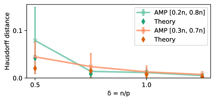
Figure 1: Hausdorff error vs. $\delta=n/p$ for two configurations.

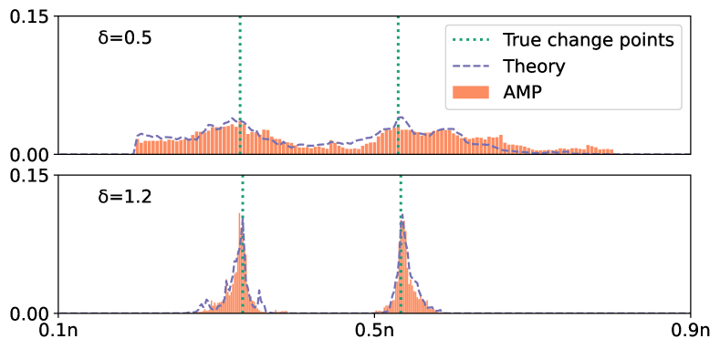
Figure 2: Approximate posterior vs. change point locations.

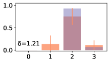
Figure 3: Approximate posterior on the number of change points $(L^{*}-1)$. $L^{*}=3,L=4$.

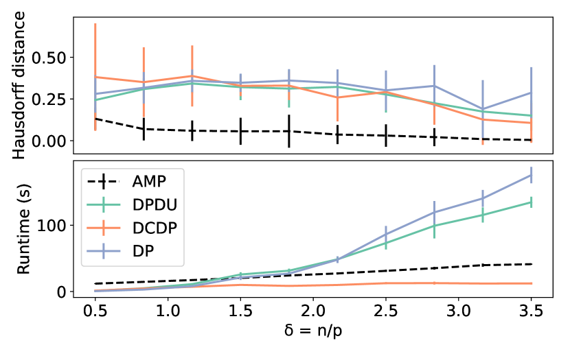
Figure 4: Comparison with $\mathtt{DPDU}$, $\mathtt{DCDP}$ and $\mathtt{DP}$ for sparse prior ${\mathbb{P}}_{\bar{\bm{B}}}=0.5{\sf N}({\bm{0}},\delta\bm{I})+0.5\delta_{{\bm{0}}}$. $L^{*}=L=3$. Runtime shown is the average runtime per set of CV parameters.

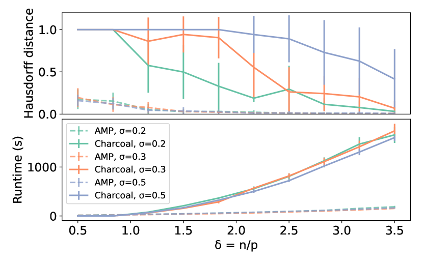
Figure 5: Comparison with $\mathtt{charcoal}$ for a sparse difference prior with sparsity level 0.5. $L^{*}=L=3$.

Figures 4 and 5 compare the performance of AMP against four state-of-the-art algorithms: the dynamic programming ($\mathtt{DP}$) approach in (Rinaldo et al., 2021); dynamic programming with dynamic updates $(\mathtt{DPDU})$ (Xu et al., 2022); divide and conquer dynamic programming ($\mathtt{DCDP}$) (Li et al., 2023); and a complementary-sketching-based algorithm called $\mathtt{charcoal}$ (Gao & Wang, 2022). Hyperparameters are chosen using cross validation (CV), as outlined in Section A.1 of (Li et al., 2023). The first three algorithms, designed for sparse signals, combine LASSO-type estimators with partitioning techniques based on dynamic programming. The $\mathtt{charcoal}$ algorithm is designed for the setting where the difference ${\bm{\beta}}^{(\eta_{\ell})}-{\bm{\beta}}^{(\eta_{\ell+1})}$ between adjacent signals is sparse. None of these algorithms uses a prior on the change point locations, unlike AMP which can flexibly incorporate both priors via ${\mathbb{P}}_{\bar{\bm{B}}}$ and $\pi_{\bar{{\bm{\Psi}}}}$.

Figure 4 uses $p=200,\sigma=0.1,\Delta=n/10,L^{*}=L=3$ and a sparse Bernoulli-Gaussian signal prior ${\mathbb{P}}_{\bar{\bm{B}}}=0.5{\sf N}({\bm{0}},\delta\bm{I})+0.5\delta_{\bm{0}}$. AMP assumes no knowledge of the true sparsity level 0.5 and estimates the sparsity level using CV over a set of values not including the ground truth (details in Appendix E). Figure 5 uses $p=300,\Delta=n/10,L^{*}=L=3$ and a Gaussian sparse difference prior with sparsity level $0.5$ (described in (88)-(90)). AMP is run assuming a mismatched sparsity level of 0.9 and a mismatched magnitude for the sparse difference vector (details in Appendix E). Figures 4 and 5 show that AMP consistently achieves the lowest Hausdorff distance among all algorithms and outperforms most algorithms in runtime. Figures 7 and 8 in Appendix E show results from an additional set of experiments comparing AMP with $\mathtt{DCDP}$ (the fastest algorithm in Figure 4). Figure 7 shows the performance of AMP with different change point priors $\pi_{\bar{{\bm{\Psi}}}}$ and suboptimal denoising functions, e.g., soft thresholding. Figure 8 demonstrates the favourable runtime scaling of AMP over $\mathtt{DCDP}$ with respect to $p$, due to the LASSO computations involved in $\mathtt{DCDP}$.

Compressed Sensing with change points

In Figure 6, we consider noiseless compressed sensing, where the signals $\{{\bm{\beta}}^{(i)}\}_{i\in[n]}$ are rotated versions of a $(255,255)$ sparse grayscale image used by Schniter & Rangan (2014). The fraction of nonzero components in the image is 8645/50625. We downsample the original image by a factor of three and flatten, yielding an operation dimension of $p=85^{2}=7225$. We set $\{{\bm{\beta}}^{(i)}\}_{i=1}^{0.3n}$ to be the image, $\{{\bm{\beta}}^{(i)}\}_{i=0.3n}^{0.7n}$ to be a $30^{\circ}$ rotated version, and $\{{\bm{\beta}}^{(i)}\}_{i=0.7n}^{n}$ to be a $45^{\circ}$ rotated version. We run AMP with a Bernoulli-Gaussian prior ${\mathbb{P}}_{\bar{\bm{B}}}$, $\Delta=n/4$ and $L=L^{*}=3$. Figure 6 shows image reconstructions along with the approximate posterior $p_{{\bm{\Psi}}|\bar{\bm{V}}_{\bm{\Theta}}^{t},q(\bm{Z},{\bm{\Psi}},\bar{\bm{\varepsilon}})}(\cdot|\bm{\Theta}^{t},\bm{y})$. The approximate posterior concentrates around the true change point locations as $\delta$ increases, even when the image reconstructions are approximate. The experiment took one hour to complete on an Apple M1 Max chip, whereas competing algorithms did not return an output within 2.5 hours, due to the larger signal dimension compared to Figure 4 ($p=7225$ vs $p=200$).

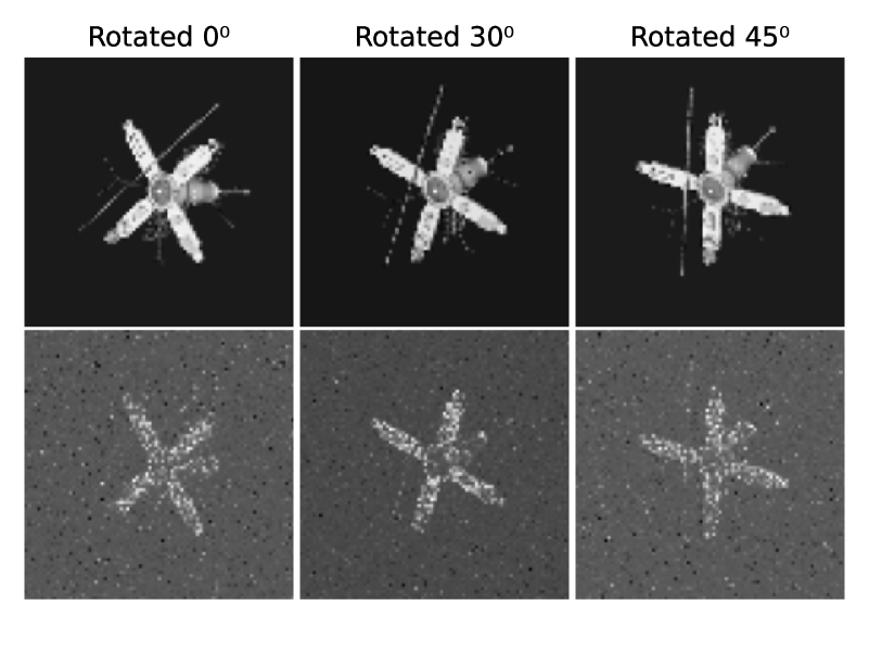
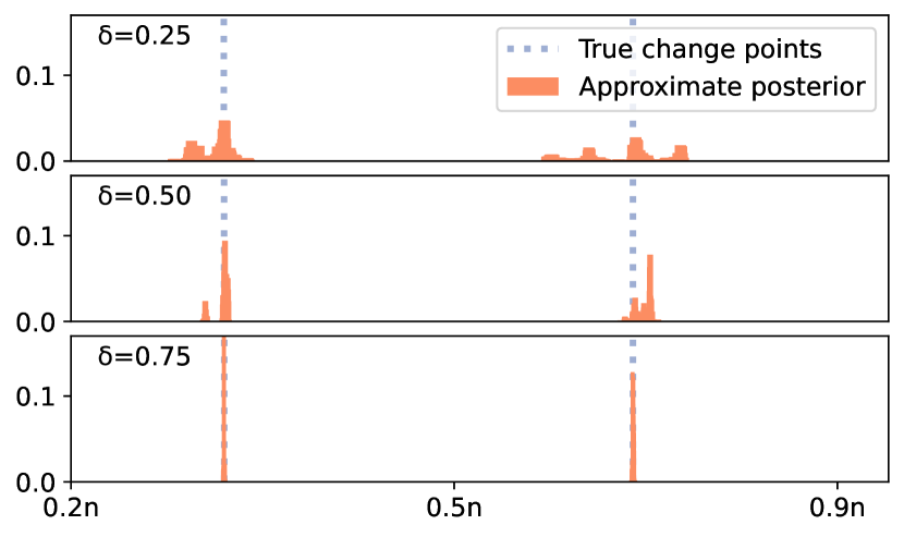
Figure 6: Top: Ground truth images (first row) and reconstruction from AMP (second row) at $\delta=0.75$. Bottom: Approximate posterior vs. fractional change point locations for different $\delta$.

Appendix A Proof of State Evolution

The proof of Theorem 3.1 relies on a generalization of Lemma 14 in (Gerbelot & Berthier, 2023), presented as Lemma A.1 below. Let $\bm{W}_{0}\in\mathbb{R}^{N\times Q}$ be a matrix such that $\|\bm{W}_{0}^{\top}\bm{W}_{0}\|_{F}/N$ converges to a finite constant as $N\to\infty$, and let $\bm{A}\in\mathbb{R}^{N\times N}$ be a symmetric GOE($N$) matrix, independent of $\bm{W}_{0}$. Then Lemma 14 in (Gerbelot & Berthier, 2023) gives a state evolution result involving an AMP iteration whose denoising function takes as input the output of the generalized linear model $\varphi(\bm{A}\bm{W}_{0})$, where $\varphi:\mathbb{R}^{N\times Q}\to\mathbb{R}^{N}$.

Lemma A.1 generalizes Lemma 14 of Gerbelot & Berthier (2023) in two ways: i) it allows for the inclusion of an auxiliary matrix ${\bm{\Xi}}\in{\mathbb{R}}^{N\times L_{{\bm{\Xi}}}}$ so that the generalized linear model in question is of the form $\varphi(\bm{A}\bm{W}_{0},{\bm{\Xi}})$, and ii) the state evolution convergence result holds for pseudo-Lipschitz test functions taking both the auxiliary matrix ${\bm{\Xi}}$ and $\bm{A}\bm{W}_{0}$ as inputs.

We extend this lemma by considering an independent random matrix ${\bm{\Xi}}\in{\mathbb{R}}^{N\times L_{{\bm{\Xi}}}}$, serving as input to a set of pseudo-Lipschitz functions $\varphi:\mathbb{R}^{N\times(Q+L_{{\bm{\Xi}}})}\to\mathbb{R}^{N}$. We then analyze a similar AMP iteration whose denoising function $\tilde{f}^{t}$ takes $\varphi(\bm{A}\bm{W}_{0},{\bm{\Xi}})$ as input instead of $\varphi(\bm{A}\bm{W}_{0})$, initialized with an independent initializer $\mathbf{X}^{0}\in\mathbb{R}^{N\times Q}$:

$$\bm{X}^{t+1}=\bm{A}\bm{M}^{t}-\bm{M}^{t-1}(\bm{b}^{t})^{\top} \in\mathbb{R}^{N\times Q}\,,$$ (32)

$$\bm{M}^{t}=\tilde{f}^{t}(\varphi\left(\bm{A}\bm{W}_{0},{\bm{\Xi}}\right),\bm{X}^{t}) \in\mathbb{R}^{N\times Q}\,,$$ (33)

$$\bm{b}^{t}=\frac{1}{N}\sum_{i=1}^{N}\frac{\partial\tilde{f}^{t}_{i}}{\partial\bm{X}_{i}^{t}}(\varphi\left(\bm{A}\bm{W}_{0},{\bm{\Xi}}\right),\bm{X}^{t}) \in\mathbb{R}^{Q\times Q}\,.$$ (34)

Our result in Lemma A.1 presents an asymptotic characterization of (32)–(34) via the following state evolution recursion:

$$\bm{\nu}^{0},\hat{{\bm{\nu}}}^{0}={\bm{0}},$$ (35)

$$\bm{\kappa}^{0,0}=\lim_{N\to\infty}\frac{1}{N}\tilde{f}^{0}(\bm{X}^{0})^{\top}\tilde{f}^{0}(\bm{X}^{0}),$$ (36)

$$\bm{\nu}^{t+1}=\lim_{N\to\infty}\frac{1}{N}\mathbb{E}\left[\bm{W}_{0}^{\top}\right.\left.\tilde{f}^{t}\left(\varphi(\bm{Z}_{\bm{W}_{0}},{\bm{\Xi}}),\bm{Z}_{\bm{W}_{0}}{\bm{\rho}}_{\bm{W}_{0}}^{-1}\bm{\nu}^{t}+\bm{W}_{0}\hat{\bm{\nu}}^{t}+\bm{Z}^{t}\right)\right],$$ (37)

$$\hat{\bm{\nu}}^{t+1}=\lim_{N\to\infty}\frac{1}{N}\mathbb{E}\left[\sum_{i=1}^{N}\partial_{1i}\bar{f}_{i}^{t}\left(\bm{Z}_{\bm{W}_{0}},\bm{Z}_{\bm{W}_{0}}{\bm{\rho}}_{\bm{W}_{0}}^{-1}\bm{\nu}^{t}+\bm{W}_{0}\hat{\bm{\nu}}^{t}+\bm{Z}^{t},{\bm{\Xi}}\right)\right],$$ (38)

$$\bm{\kappa}^{t+1,s+1}=\bm{\kappa}^{s+1,t+1}=\lim_{N\to\infty}\frac{1}{N}\mathbb{E}\left[\left(\tilde{f}^{s}\left(\varphi(\bm{Z}_{\bm{W}_{0}},{\bm{\Xi}}),\bm{Z}_{\bm{W}_{0}}{\bm{\rho}}_{\bm{W}_{0}}^{-1}\bm{\nu}^{s}+\bm{W}_{0}\hat{\bm{\nu}}^{s}+\bm{Z}^{s}\right)-\bm{W}_{0}{\bm{\rho}}_{\bm{W}_{0}}^{-1}\bm{\nu}^{s+1}\right)^{\top}\right.$$

$$\left.\hskip 170.71652pt\left(\tilde{f}^{t}\left(\varphi(\bm{Z}_{\bm{W}_{0}},{\bm{\Xi}}),\bm{Z}_{\bm{W}_{0}}{\bm{\rho}}_{\bm{W}_{0}}^{-1}\bm{\nu}^{t}+\bm{W}_{0}\hat{\bm{\nu}}^{t}+\bm{Z}^{t}\right)-\bm{W}_{0}{\bm{\rho}}_{\bm{W}_{0}}^{-1}\bm{\nu}^{t+1}\right)\right],$$ (39)

where ${\bm{\rho}}_{\bm{W}_{0}}=\lim_{N\to\infty}\frac{1}{N}\bm{W}_{0}^{\top}\bm{W}_{0}$, and for $i\in[n]$ we have $(\bm{Z}_{\bm{W}_{0}})_{i}\mathbin{\overset{i.i.d}{\kern 0.0pt\sim}}{\sf N}(\bm{0},{\bm{\rho}}_{\bm{W}_{0}})$. For $i\in[n],0\leq s,r\leq t$, we have that $(\bm{Z}_{\bm{W}_{0}})_{i}$ is independent from $({\bm{Z}}^{s})_{i}\mathbin{\overset{i.i.d}{\kern 0.0pt\sim}}{\sf N}\left({\bm{0}},{\bm{\kappa}}^{s,s}\right)$ with ${\rm{{Cov}}}(({\bm{Z}}^{s})_{i},({\bm{Z}}^{r})_{i})={\bm{\kappa}}^{s,r}$. In (38), we let $\bar{f}^{t}:(\bm{z},\bm{u},\bm{v})\mapsto\tilde{f}^{t}(\varphi(\bm{z},\bm{v}),\bm{u})$ and we let $\partial_{1i}\bar{f}_{i}^{t}$ denote the partial derivative of $\bar{f}_{i}^{t}$ with respect to the $i$-th row of its first argument.

We list the necessary assumptions for characterizing this AMP iteration, followed by the result:

Assumptions.

1. $\bm{A}\in\mathbb{R}^{N\times N}$ is a GOE($N$) matrix, i.e., $\bm{A}=\mathbf{G}+\mathbf{G}^{\top}$ for $\mathbf{G}\in\mathbb{R}^{N\times N}$ with i.i.d. entries $G_{ij}\sim{\sf N}(0,1/(2N))$.

2. For each $t\in\mathbb{N}_{>0}$, $\bar{f}^{t}:(\bm{z},\bm{u},{\bm{\Xi}})\mapsto\tilde{f}^{t}(\varphi(\bm{z},{\bm{\Xi}}),\bm{u})$ is uniformly pseudo-Lipschitz. For each $t\in\mathbb{N}_{>0}$ and for any $1\leqslant i\leqslant N$, $(\bm{u},\bm{z})\mapsto\frac{\partial\tilde{f}^{t}_{i}}{\partial\bm{X}_{i}}(\varphi(\bm{z},{\bm{\Xi}}),\bm{u})$ is uniformly pseudo-Lipschitz. The function $\tilde{f}^{0}:\mathbb{R}^{N\times Q}\to\mathbb{R}^{N\times Q}$ is uniformly pseudo-Lipschitz.

3. The initialization $\bm{X}^{0}$ is deterministic, and $\|\bm{X}^{0}\|_{F}/\sqrt{N}$, $\|{\bm{W}_{0}^{\top}\bm{W}_{0}}\|_{2}/N$, $\|{{\bm{\Xi}}}\|_{F}/\sqrt{N}$ converge almost surely to finite constants as $N\to\infty$.

4. The following limits exist and are finite:

   $$\lim_{N\to\infty}\frac{1}{N}\tilde{f}^{0}(\bm{X}^{0})^{\top}\tilde{f}^{0}(\bm{X}^{0}),\quad\lim_{N\to\infty}\frac{1}{N}\bm{W}_{0}^{\top}\tilde{f}^{0}(\bm{X}^{0}).$$

5. For any $t\in\mathbb{N}_{>0}$ and any $\bm{\kappa}\in{\mathcal{S}}_{Q}^{+}$, the following limit exists and is finite:

   $$\lim_{N\to\infty}\frac{1}{N}\mathbb{E}\left[\tilde{f}^{0}(\bm{X}^{0})^{\top}\tilde{f}^{t}(\varphi(\bm{Z},{\bm{\Xi}}),{\bm{Z}})\right]$$

   where $\bm{Z}\in\mathbb{R}^{N\times Q}$, $\bm{Z}\sim{\sf N}\left(0,\bm{\kappa}\otimes\mathbf{I}_{N}\right)$.

6. For any $s,t\in\mathbb{N}_{>0}$ and any $\bm{\kappa}\in{\mathcal{S}}_{2Q}^{+}$, the following limit exists and is finite:

   $$\lim_{N\to\infty}\frac{1}{N}\mathbb{E}\left[\tilde{f}^{s}(\varphi(\bm{Z}^{s},{\bm{\Xi}}),{\bm{Z}}^{s})^{\top}\tilde{f}^{t}(\varphi(\bm{Z}^{t},{\bm{\Xi}}),{\bm{Z}}^{t})\right]$$

   where $(\bm{Z}^{s},\bm{Z}^{t})\in(\mathbb{R}^{N\times Q})^{2}$,$(\bm{Z}^{s},\bm{Z}^{t})\sim{\sf N}(0,\bm{\kappa}\otimes\mathbf{I}_{N})$.

Lemma A.1.

Consider the AMP iteration (32)–(34) and the state evolution recursion (35)–(A). Assume $\ref{it:ass-sym-1}-\ref{it:ass-sym-6}$. Then for any sequence of functions $\Phi_{N}:(\mathbb{R}^{N\times Q})^{\otimes(t+3)}\times{\mathbb{R}}^{N\times L_{{\bm{\Xi}}}}\to\mathbb{R}$ such that $(\bm{X}^{0},\dots,\bm{X}^{t},\bm{V})\mapsto\Phi_{N}(\mathbf{X}^{0},\mathbf{X}^{1},...,\mathbf{X}^{t},\bm{V},\bm{W}_{0},{\bm{\Xi}})$ is uniformly pseudo-Lipschitz, we have that:

$$\Phi_{N}\left(\mathbf{X}^{0},\mathbf{X}^{1},...,\mathbf{X}^{t},\bm{A}\bm{W}_{0},\bm{W}_{0},{\bm{\Xi}}\right)$$

$$\hskip 28.45274pt\stackrel{{\scriptstyle{\mathbb{P}}}}{{\simeq}}{\mathop{\mathbb{E}}}_{\bm{Z}^{0},\dots,\bm{Z}^{t},\bm{Z}_{\bm{W}_{0}}}\left[\Phi_{N}\left(\bm{Z}_{\bm{W}_{0}}{\bm{\rho}}_{\bm{W}_{0}}^{-1}\bm{\nu}^{0}+\bm{W}_{0}\hat{\bm{\nu}}^{0}+\bm{Z}^{0},\dots,\bm{Z}_{\bm{W}_{0}}{\bm{\rho}}_{\bm{W}_{0}}^{-1}\bm{\nu}^{t}+\bm{W}_{0}\hat{\bm{\nu}}^{t}+\bm{Z}^{t},\bm{Z}_{\bm{W}_{0}},\bm{W}_{0},{\bm{\Xi}}\right)\right].$$ (40)

Proof.

The main differences between the AMP result in (Gerbelot & Berthier, 2023) and our characterization are: 1) the $\varphi$ function is allowed to depend on an auxiliary random variable ${\bm{\Xi}}$, 2) the test function $\Phi_{N}$ is allowed to depend additionally on $\bm{A}\bm{W}_{0}$, $\bm{W}_{0}$, and ${\bm{\Xi}}$. Assumption (B2) guarantees that $\tilde{f}^{t}$ maintains the same required coverage properties despite modification $1)$.

We now address modification 2). Since ${\bm{\Xi}}$ and $\bm{W}_{0}$ are fixed and $\tilde{\Phi}_{N}:(\bm{X}^{0},\dots,\bm{X}^{t},\bm{V})\mapsto\Phi_{N}(\mathbf{X}^{0},\mathbf{X}^{1},...,\mathbf{X}^{t},\bm{V},\bm{W}_{0},{\bm{\Xi}})$ is assumed to be uniformly pseudo-Lipschitz, these can be included in $\Phi_{N}$ and the right hand side of (40) is unaffected. Further, note that by Proposition 2 in (Gerbelot & Berthier, 2023) (a standard upper bound on the operator norm of $\bm{A}\mathbin{\overset{}{\kern 0.0pt\sim}}GOE(N)$) we have that $\|\bm{A}\bm{W}_{0}\|_{F}/\sqrt{N}<\infty$ as $N\to\infty$. We can therefore include $\bm{A}\bm{W}_{0}$ in the definition of $\Phi_{N}$ as well, and the uniform pseudo-Lipschitzness of $\tilde{\Phi}_{N}$ guarantees convergence to the result. ∎

We next present the main reduction, mapping the AMP algorithm proposed in this work (LABEL:eq:amp) to the symmetric one outlined in (32)–(34).

Proof of Theorem 3.1.

Consider the Change Point Linear Regression model (1), and recall that it can be rewritten as (2). We reduce the algorithm (LABEL:eq:amp) to (32)–(34), following the alternating technique of (Javanmard & Montanari, 2013). The idea is to define a symmetric GOE matrix with $\bm{X}$ and $\bm{X}^{\top}$ on the off-diagonals. With a suitable initialization, the iteration (32)–(34) then yields $\bm{B}^{t+1}$ in the even iterations and for $\bm{\Theta}^{t}$ in the odd iterations.

Let $N=n+p$. For a matrix ${\bm{E}}\in{\mathbb{R}}^{N\times L}$, we use ${\bm{E}}_{[n]}$ and ${\bm{E}}_{[-p]}$ to denote the first $n$ rows and the last $p$ rows of ${\bm{E}}$ respectively. Recall from (LABEL:eq:amp) that $\bm{X}\in\mathbb{R}^{n\times p},\bm{B},\bm{B}^{t}\in\mathbb{R}^{p\times L}$ and $\bm{\Theta}=\bm{X}\bm{B},\bm{\Theta}^{t}\in\mathbb{R}^{n\times L}$, and $n/p\to\delta$ as $n,p\to\infty$. We let

$$\bm{A}=\sqrt{\frac{\delta}{\delta+1}}\begin{bmatrix}\bm{D}_{1}&\bm{X}\\ \bm{X}^{\top}&\bm{D}_{2}\end{bmatrix}\sim\text{GOE}(N),\quad\bm{W}_{0}=\begin{bmatrix}\bm{0}_{n\times L}\\ \bm{B}\end{bmatrix}\in\mathbb{R}^{N\times L},\quad\bm{X}^{0}=\begin{bmatrix}\bm{0}_{n\times L}\\ \bm{B}^{0}\end{bmatrix}$$ (41)

where $\bm{D}_{1}\sim$ GOE($n$) and $\sqrt{\delta}\bm{D}_{2}\sim$ GOE($p$) are independent of each other and of $\bm{X}$. Let ${\bm{\Xi}}:=\begin{bmatrix}{\bm{\Psi}}&\bm{\varepsilon}\end{bmatrix}\in{\mathbb{R}}^{n\times 2}$ and define

$$\varphi:(\bm{W},{\bm{\Xi}})\mapsto q\left(\sqrt{\frac{\delta+1}{\delta}}\bm{W}_{[n]},{\bm{\Psi}},\bm{\varepsilon}\right)\in{\mathbb{R}}^{N},$$ (42)

for any $\bm{W}\in{\mathbb{R}}^{N\times L}$. We therefore have $\varphi(\bm{A}\bm{W}_{0},{\bm{\Xi}})=q\left(\bm{X}\bm{B},{\bm{\Psi}},\bm{\varepsilon}\right)$. Let $\tilde{f}^{t}:{\mathbb{R}}^{N\times L}\times{\mathbb{R}}^{N}\to{\mathbb{R}}^{N\times L}$ such that

$$\tilde{f}^{2t+1}(\varphi(\bm{A}\bm{W}_{0},{\bm{\Xi}}),\bm{U})=\sqrt{\frac{\delta+1}{\delta}}\begin{bmatrix}g^{t}(\bm{U}_{[n]},q(\bm{X}\bm{B},{\bm{\Psi}},\bm{\varepsilon}))\\ {\bm{0}}_{p\times L}\end{bmatrix}\quad\text{and}\quad\tilde{f}^{2t}(\varphi(\bm{A}\bm{W}_{0},{\bm{\Xi}}),\bm{U})=\sqrt{\frac{\delta+1}{\delta}}\begin{bmatrix}\bm{0}_{n\times L}\\ f^{t}(\bm{U}_{[-p]})\end{bmatrix},$$ (43)

for any $\bm{U}$ in ${\mathbb{R}}^{N\times L}$.

Next, consider the AMP iteration (32)–(34) with $\bm{A},\bm{W}_{0},\bm{X}^{0},{\bm{\Xi}},\varphi,\tilde{f}^{t}$ defined as in (41)–(43). Note that the assumptions $\ref{it:ass-sym-1}-\ref{it:ass-sym-6}$ are satisfied by construction, and hence the state evolution result in Lemma A.1 holds for the iteration (32)–(34). We will now show that the state evolution equations decompose into those of interest, (7)–(10). First, note that

$$\bm{X}^{2t+1} =\begin{bmatrix}\bm{X}f^{t}(\bm{X}^{2t}_{[-p]})-g^{t-1}(\bm{X}^{2t-1}_{[n]},q(\bm{X}\bm{B},{\bm{\Xi}}))\cdot\overbrace{\frac{1}{n}\left(\sum_{i=1}^{p}\frac{\partial{f^{t}(\bm{X}^{2t}_{[-p]})_{i}}}{\partial{\bm{X}^{2t}_{[-p],i}}}\right)^{\top}}^{=(\bm{F}^{t})^{\top}}\\ \bm{D}_{2}f^{t}(\bm{X}^{2t}_{[-p]})\end{bmatrix},$$ (44)

$$\bm{X}^{2t} =\begin{bmatrix}\bm{D}_{1}g^{t-1}(\bm{X}^{2t-1}_{[n]},q(\bm{X}\bm{B},{\bm{\Xi}}))\\ \bm{X}^{\top}g^{t-1}(\bm{X}^{2t-1}_{[n]},q(\bm{X}\bm{B},{\bm{\Xi}}))-f^{t-1}(\bm{X}^{2t-2}_{[-p]})\cdot\underbrace{\left(\frac{1}{n}\sum_{i=1}^{n}\frac{\partial{g^{t-1}(\bm{X}^{2t-1}_{[n]},q(\bm{X}\bm{B},{\bm{\Xi}}))}}{\partial{\bm{X}^{2t-1}_{[n],i}}}\right)^{\top}}_{=(\bm{C}^{t-1})^{\top}}\end{bmatrix},$$ (45)

and hence observe that $\bm{X}^{2t+1}_{[n]}$ and $\bm{X}^{2t}_{[-p]}$ are equal to $\bm{\Theta}^{t}$ and $\bm{B}^{t}$ in (LABEL:eq:amp) respectively. Define the main iterate ${\bm{Q}}^{t}=\bm{Z}_{\bm{W}_{0}}{\bm{\rho}}^{-1}_{\bm{W}_{0}}{\bm{\nu}}^{t}+\bm{W}_{0}\hat{{\bm{\nu}}}^{t}+\bm{Z}^{t}\in\mathbb{R}^{N\times L}$. For $i\in[n]$, let $\tilde{g}_{i}^{t}:(\bm{Z},\bm{V},{\bm{\Psi}},\bm{\varepsilon})\mapsto g_{i}^{t}(\bm{V},q(\bm{Z},{\bm{\Psi}},\bm{\varepsilon}))$ and let $\partial_{1i}\tilde{g}_{i}^{t}$ be the partial derivative (Jacobian) w.r.t. the $i$th row of the first argument. Following (35)–(A), we then have that

$${\bm{\nu}}^{2t+1}=\lim_{N\to\infty}\frac{1}{N}\sqrt{\frac{\delta+1}{\delta}}{\mathop{\mathbb{E}}}\left[{\begin{bmatrix}{\bm{0}}_{L\times n}&\bm{B}^{\top}\end{bmatrix}}{\begin{bmatrix}{\bm{0}}_{n\times L}\\ f^{t}({\bm{Q}}^{2t}_{[-p]})\end{bmatrix}}\right]=\sqrt{\frac{\delta}{\delta+1}}\lim_{n\to\infty}\frac{1}{n}{\mathop{\mathbb{E}}}\left[\bm{B}^{\top}f^{t}({\bm{Q}}^{2t}_{[-p]})\right],$$ (46)

$${\bm{\nu}}^{2t}=\sqrt{\frac{\delta+1}{\delta}}\lim_{N\to\infty}\frac{1}{N}{\mathop{\mathbb{E}}}\left[{\begin{bmatrix}{\bm{0}}_{L\times n}&\bm{B}^{\top}\end{bmatrix}}{\begin{bmatrix}g^{t-1}({\bm{Q}}_{[n]}^{2t-1},\bm{Y})\\ {\bm{0}}_{p\times L}\end{bmatrix}}\right]={\bm{0}}_{L\times L},$$ (47)

$$\hat{{\bm{\nu}}}^{2t+1}={\bm{0}}_{L\times L}$$ (48)

$$\hat{{\bm{\nu}}}^{2t}=\lim_{n\to\infty}\frac{1}{n}{\mathop{\mathbb{E}}}\left[\sum_{i=1}^{n}\partial_{1i}{\tilde{g}^{t-1}_{i}\left(\sqrt{\frac{\delta+1}{\delta}}\bm{Z}_{\bm{W}_{0},[n]},{\bm{Q}}^{2t-1}_{[n]},{\bm{\Psi}},\bm{\varepsilon}\right)}\right],$$ (49)

$${\bm{\kappa}}^{2t,2s}=\lim_{n\to\infty}\frac{1}{n}{\mathop{\mathbb{E}}}\left[g^{t-1}\left({\bm{Q}}^{2t-1}_{[n]},q\left(\sqrt{\frac{\delta+1}{\delta}}\bm{Z}_{\bm{W}_{0},[n]},{\bm{\Psi}},\bm{\varepsilon}\right)\right)^{\top}g^{s-1}\left({\bm{Q}}^{2s-1}_{[n]},q\left(\sqrt{\frac{\delta+1}{\delta}}\bm{Z}_{\bm{W}_{0},[n]},{\bm{\Psi}},\bm{\varepsilon}\right)\right)\right]$$ (50)

$${\bm{\kappa}}^{2t+1,2s+1}=\lim_{n\to\infty}\frac{1}{n}{\mathop{\mathbb{E}}}\left[\left(f^{t}({\bm{Q}}_{[-p]}^{2t})-\sqrt{\frac{\delta+1}{\delta}}\bm{B}{\bm{\rho}}_{\bm{B}}^{-1}{\bm{\nu}}^{2t+1}\right)^{\top}\left(f^{s}({\bm{Q}}_{[-p]}^{2s})-\sqrt{\frac{\delta+1}{\delta}}\bm{B}{\bm{\rho}}_{\bm{B}}^{-1}{\bm{\nu}}^{2s+1}\right)\right],$$ (51)

where in (51) we used ${\bm{\rho}}_{\bm{W}_{0}}=\frac{1}{N}{\bm{B}}^{\top}{\bm{B}}=\frac{\delta}{\delta+1}{\bm{\rho}}_{\bm{B}}$. Hence, we can associate

$${\bm{\nu}}^{t}_{\bm{\Theta}} =\sqrt{\frac{\delta+1}{\delta}}{\bm{\nu}}^{2t+1},$$ (52)

$${{\bm{\nu}}}^{t}_{\bm{B}} =\hat{{\bm{\nu}}}^{2t},$$ (53)

$${\bm{\kappa}}_{\bm{\Theta}}^{t,s} ={\bm{\kappa}}^{2t+1,2s+1},$$ (54)

$${\bm{\kappa}}_{\bm{B}}^{t,s} ={\bm{\kappa}}^{2t,2s}.$$ (55)

$$\bm{Z}_{\bm{B}} \stackrel{{\scriptstyle d}}{{=}}\sqrt{\frac{\delta+1}{\delta}}\bm{Z}_{\bm{W}_{0},[n]},$$ (56)

$$\bm{G}^{t}_{\bm{\Theta}} \stackrel{{\scriptstyle d}}{{=}}\bm{Z}^{2t+1}_{[n]},$$ (57)

$$\bm{G}^{t}_{\bm{B}} \stackrel{{\scriptstyle d}}{{=}}\bm{Z}^{2t}_{[-p]},$$ (58)

$$\bm{V}^{t}_{\bm{\Theta}} \stackrel{{\scriptstyle d}}{{=}}{\bm{Q}}^{2t+1}_{[n]},$$ (59)

$$\bm{V}^{t}_{\bm{B}} \stackrel{{\scriptstyle d}}{{=}}{\bm{Q}}^{2t}_{[-p]}.$$ (60)

Substituting the change of variables (52)–(60) into (46)–(51), we obtain (7)–(10). Moreover, substituting (44)–(45) and (59)–(60) into Lemma A.1 yields Theorem 3.1. ∎

Appendix B State Evolution Limits and Simplifications

B.1 State Evolution Dependence on $\bm{B},\bm{\varepsilon}$

In this section, we outline how the limits in (7)–(10) can be checked, and how the dependence of (7)–(10) on $\bm{B},\bm{\varepsilon}$ can be removed. We give a set of sufficient conditions for the existence of the limits in (7)–(10), which allow for removing the dependency of the state evolution (7)–(10) on $\bm{B},\bm{\varepsilon}$. Assume (S0) on p.(S0), and also that the following assumptions hold:

1. As $n\to\infty$, the entries of the normalized change point vector ${\bm{\eta}}/n$ converge to constants $\alpha_{0},\dots,\alpha_{L}$ such that $0=\alpha_{0}<\alpha_{1}<\dots<\alpha_{L^{*}}=\ldots=\alpha_{L}=1$.

2. For $t\geq 0$, $f^{t}$ is separable, and $g^{t}$ acts row-wise on its input. (We recall that a separable function acts row-wise and identically on each row.)

3. For $\ell\in[L^{*}-1]$, the empirical distributions of $\{\tilde{g}_{i}^{t}(\bm{Z}_{1},(\bm{V}^{t}_{\bm{\Theta}})_{1},\Psi_{\eta_{\ell}},\varepsilon_{i})\}_{i\in[\eta_{\ell},\eta_{\ell+1})}$ and $\{\partial_{1}{\tilde{g}_{i}^{t}(\bm{Z}_{1},(\bm{V}^{t}_{\bm{\Theta}})_{1},\Psi_{\eta_{\ell}},\varepsilon_{i})}\}_{i\in[\eta_{\ell},\eta_{\ell+1})}$ converge weakly to the laws of random variables $\hat{g}^{t}_{\eta_{\ell}}(\bm{Z}_{1},(\bm{V}^{t}_{\bm{\Theta}})_{1},\Psi_{\eta_{\ell}},,\bar{\varepsilon}))$ and ${\check{g}^{t}}_{\eta_{\ell}}(\bm{Z}_{1},(\bm{V}_{\bm{\Theta}}^{t})_{1},\Psi_{\eta_{\ell}},\bar{\varepsilon})$, respectively, where $\partial_{1}$ denotes Jacobian with respect to the first argument.

The assumption (S1) is natural in the regime where the number of samples $n$ is proportional to $p$, and the number of degrees of freedom in the signals also grows linearly in $p$. Without change points, $f^{t},g^{t}$ can both be assumed separable without loss of optimality (due to (S0)). To handle the temporal dependence created by change points, we require $g^{t}_{i}$ to depend on $i$, for $i\in[n]$. However, Proposition 3.2 shows that it can be chosen to act row-wise, i.e., $g^{*t}_{i}(\bm{\Theta}^{t},{\bm{y}})=g^{*t}_{i}(\bm{\Theta}^{t}_{i},y_{i})$. This justifies (S2). When $g_{i}^{t}$ is chosen to be $g_{i}^{*t}$ for $i\in[n]$, the condition (S3) can be translated into regularity conditions on the prior marginals $\pi_{\bar{\Psi}_{i}}$ and distributional convergence conditions on the noise $\varepsilon_{i}$, as these are the only quantities that differ along the elements of the sets $\{\tilde{g}_{i}^{t}(\bm{Z}_{1},(\bm{V}^{t}_{\bm{\Theta}})_{1},\Psi_{\eta_{\ell}},\varepsilon_{i})\}_{i\in[\eta_{\ell},\eta_{\ell+1})}$ and $\{\partial_{1}{\tilde{g}_{i}^{t}(\bm{Z}_{1},(\bm{V}^{t}_{\bm{\Theta}})_{1},\Psi_{\eta_{\ell}},\varepsilon_{i})}\}_{i\in[\eta_{\ell},\eta_{\ell+1})}$ for $\ell\in[L^{*}-1]$.

Under assumptions (S0)-(S3), the state evolution equations in (7)–(10) reduce to:

$${{\bm{\nu}}}_{\bm{B}}^{t+1}=\sum_{\ell=0}^{L-1}{\mathop{\mathbb{E}}}\left[{\check{g}^{t}}_{\eta_{\ell}}(\bm{Z}_{1},(\bm{V}_{\bm{\Theta}}^{t})_{1},\Psi_{\eta_{\ell}},\bar{\varepsilon})\right],$$ (61)

$${\bm{\kappa}}_{\bm{B}}^{s+1,t+1}=\sum_{\ell=0}^{L-1}{\mathop{\mathbb{E}}}\left[\hat{g}^{s}_{\eta_{\ell}}((\bm{V}_{\bm{\Theta}}^{s})_{1},q_{1}(\bm{Z}_{1},\Psi_{\eta_{\ell}},\bar{\varepsilon}))\ \hat{g}^{t}_{\eta_{\ell}}((\bm{V}_{\bm{\Theta}}^{t})_{1},q_{1}(\bm{Z}_{1},\Psi_{\eta_{\ell}},\bar{\varepsilon}))^{\top}\right],$$ (62)

$${\bm{\nu}}^{t+1}_{\bm{\Theta}}=\frac{1}{\delta}{\mathop{\mathbb{E}}}\left[\bar{\bm{B}}f^{t+1}_{1}(({{\bm{\nu}}}^{t+1}_{\bm{B}})^{\top}\bar{\bm{B}}+(\bm{G}^{t+1}_{\bm{B}})_{1})^{\top}\right],$$ (63)

$${\bm{\kappa}}_{\bm{\Theta}}^{s+1,t+1}=\frac{1}{\delta}{\mathop{\mathbb{E}}}\left[\left(f^{s+1}_{1}(({{\bm{\nu}}}^{s+1}_{\bm{B}})^{\top}\bar{\bm{B}}+({\bm{G}}^{s+1}_{\bm{B}})_{1})-({\bm{\nu}}^{s+1}_{\bm{\Theta}})^{\top}{\bm{\rho}}^{-1}\bar{\bm{B}}\right)\right.$$

$$\hskip 199.16928pt\left.\left(f^{t+1}_{1}(({{\bm{\nu}}}^{t+1}_{\bm{B}})^{\top}\bar{\bm{B}}+(\bm{G}^{t+1}_{\bm{B}})_{1})-({\bm{\nu}}^{t+1}_{\bm{\Theta}})^{\top}{\bm{\rho}}^{-1}\bar{\bm{B}}\right)^{\top}\right],$$ (64)

where (S2) has allowed us to reduce the matrix products into sums of vector outer-products, and assumptions (S0)–(S3) have removed the dependence on $\bm{B}$ and $\bm{\varepsilon}$ due to the law of large numbers argument in Lemma 4 of (Bayati & Montanari, 2011).

B.2 Removing dependencies on $\bm{\varepsilon}$ on the RHS of (28)–(29)

Under assumptions (S0)–(S3) above, the dependence of $\bm{V}_{\bm{\Theta}}^{t}$ on the RHS of (28)–(29) on $\bm{B},\bm{\varepsilon}$ can be removed. Moreover, the dependence of the RHS on $\bm{\varepsilon}$ through $\hat{{\bm{\eta}}}$ can be removed on a case-by-case basis. We expect this to hold, for example, under (S0)–(S3) for estimators whose dependence on $\bm{\varepsilon}$ is via a normalized inner product such as (27):

$$U(\hat{{\bm{\eta}}}(\bm{V}_{\bm{\Theta}}^{t},q(\bm{Z},U({\bm{\eta}}),\bm{\varepsilon})))=\operatorname*{arg\,max}_{\psi\in\mathcal{X}}\frac{\langle(\bm{V}_{\bm{\Theta}}^{t})_{[:,{\bm{\psi}}]},\bm{Z}_{[:,{\bm{\psi}}]}\rangle}{n}+\frac{\langle(\bm{V}_{\bm{\Theta}}^{t})_{[:,{\bm{\psi}}]},\bm{\varepsilon}\rangle}{n}.$$ (65)

Indeed, the numerical experiments in Section 4 for chosen estimators demonstrate a strong agreement between the left-hand and right-hand sides of (28) and of (31), when $\bm{\varepsilon}$ on the right-hand side is substituted by an independent copy with the same limiting moments.

Appendix C Proof and Computation of Optimal Denoisers $f^{t},g^{t}$

C.1 Proof of Proposition 3.2

It is similar to the derivation of the optimal denoisers for mixed regression in (Tan & Venkataramanan, 2023), with a few differences in the derivation of $g^{*t}$. We include both parts here for completeness. This proof relies on Lemma C.1 and Lemma C.2, Cauchy-Schwarz inequality and Stein’s Lemma extended to vector or matrix random variables. Recall that we treat vectors, including rows of matrices, as column vectors, and that functions $h:\mathbb{R}^{q}\to\mathbb{R}^{q}$ have column vectors as input and output.

Lemma C.1 (Extended Cauchy-Schwarz inequality, Lemma 2 in (Lavergne, 2008)).

Let ${\bm{A}}\in{\mathbb{R}}^{n\times L}$ and ${\bm{B}}\in{\mathbb{R}}^{n\times L}$ be random matrices such that ${\mathop{\mathbb{E}}}\|{\bm{A}}\|_{F}^{2}<\infty,{\mathop{\mathbb{E}}}\|{\bm{B}}\|_{F}^{2}<\infty,$ and ${\mathop{\mathbb{E}}}[\bm{A}^{\top}\bm{A}]$ is non-singular, then

$${\mathop{\mathbb{E}}}[\bm{B}^{\top}\bm{B}]-{\mathop{\mathbb{E}}}[\bm{B}^{\top}\bm{A}]({\mathop{\mathbb{E}}}[\bm{A}^{\top}\bm{A}])^{-1}{\mathop{\mathbb{E}}}[\bm{A}^{\top}\bm{B}]\succcurlyeq 0.$$ (66)

Lemma C.2 (Extended Stein’s Lemma).

Let $\bm{x}\in{\mathbb{R}}^{L}$ and $h:{\mathbb{R}}^{L}\to{\mathbb{R}}^{L}$ be such that for $\ell\in[L]$, the function $h_{\ell}:x_{\ell}\to[h(\bm{x})]_{\ell}$ is absolutely continuous for Lebesgue almost every $(x_{i}:i\neq\ell)\in{\mathbb{R}}^{L-1}$, with weak derivative $\partial h_{\ell}(\bm{x})/\partial x_{\ell}:{\mathbb{R}}^{L}\to{\mathbb{R}}$ satisfying ${\mathop{\mathbb{E}}}|\partial h_{\ell}({\bm{x}})/\partial{x}_{\ell}|<\infty$. If ${\bm{x}}\sim{\sf N}(\bm{\mu},{\bm{\Sigma}})$ with $\bm{\mu}\in{\mathbb{R}}^{L}$ and ${\bm{\Sigma}}\in{\mathbb{R}}^{L\times L}$ positive definite, then

$${\mathop{\mathbb{E}}}\left[(\bm{x}-\bm{\mu})h(\bm{x})^{\top}\right]={\bm{\Sigma}}\,{\mathop{\mathbb{E}}}[h^{\prime}(\bm{x})]^{\top},$$ (67)

where $h^{\prime}(\bm{x})$ is the Jacobian matrix of $h$.

The proof of Lemma C.2 follows from Lemma 6.20 of (Feng et al., 2022).

Proof of part 1 (optimal $f^{t}$).

Using the law of total expectation and applying (25), we can rewrite $\bar{{\bm{\nu}}}_{\bm{\Theta}}^{t}$ in (19) as:

$$\bar{{\bm{\nu}}}_{\bm{\Theta}}^{t} =\frac{1}{\delta}\lim_{p\to\infty}\frac{1}{p}\sum_{j=1}^{p}{\mathop{\mathbb{E}}}\left[\bar{\bm{B}}\left(f_{j}^{t}(\bar{\bm{V}}_{\bm{B}}^{t})\right)^{\top}\right]=\frac{1}{\delta}{\mathop{\mathbb{E}}}\left[\bar{\bm{B}}\left(f_{j}^{t}(\bar{\bm{V}}_{\bm{B}}^{t})\right)^{\top}\right]=\frac{1}{\delta}{\mathop{\mathbb{E}}}\left[{\mathop{\mathbb{E}}}\left[\bar{\bm{B}}\left(f_{j}^{t}(\bar{\bm{V}}_{\bm{B}}^{t})\right)^{\top}\big{|}\bar{\bm{V}}_{\bm{B}}^{t}\right]\right]$$

$$=\frac{1}{\delta}{\mathop{\mathbb{E}}}\left[{\mathop{\mathbb{E}}}\left[\bar{\bm{B}}|\bar{\bm{V}}_{\bm{B}}^{t}\right]\left(f_{j}^{t}(\bar{\bm{V}}_{\bm{B}}^{t})\right)^{\top}\right]=\frac{1}{\delta}{\mathop{\mathbb{E}}}\left[f_{j}^{*t}(f_{j}^{t})^{\top}\right],$$ (68)

where we used the shorthand $f_{j}^{t}\equiv f_{j}^{t}(\bar{\bm{V}}_{\bm{B}}^{t})$ and $f_{j}^{*t}\equiv f_{j}^{*t}(\bar{\bm{V}}_{\bm{B}}^{t})={\mathop{\mathbb{E}}}[\bar{\bm{B}}|\bar{\bm{V}}_{\bm{B}}^{t}]$. Applying Lemma C.1 yields

$${\mathop{\mathbb{E}}}\left[f_{j}^{*t}(f_{j}^{*t})^{\top}\right]-{\mathop{\mathbb{E}}}\left[f_{j}^{*t}(f_{j}^{t})^{\top}\right]{\mathop{\mathbb{E}}}\left[f_{j}^{t}(f_{j}^{t})^{\top}\right]^{-1}{\mathop{\mathbb{E}}}\left[f_{j}^{t}(f_{j}^{*t})^{\top}\right]\succcurlyeq 0.$$ (69)

Since (20) can be simplified into

$$\bar{{\bm{\kappa}}}_{\bm{\Theta}}^{t,t}=\frac{1}{\delta}{\mathop{\mathbb{E}}}\left[f_{j}^{t}(f_{j}^{t})^{\top}\right]-(\bar{{\bm{\nu}}}_{\bm{\Theta}}^{t})^{\top}{\bm{\rho}}^{-1}{\bm{\nu}}_{\bm{\Theta}}^{t},$$ (70)

using (68) and (70) in (69), we obtain that

$${\bm{\Delta}}:=\frac{1}{\delta}{\mathop{\mathbb{E}}}\left[f_{j}^{*t}(f_{j}^{*t})^{\top}\right]-\bar{{\bm{\nu}}}_{\bm{\Theta}}^{t}\left[\bar{{\bm{\kappa}}}_{\bm{\Theta}}^{t,t}+(\bar{{\bm{\nu}}}_{\bm{\Theta}}^{t})^{\top}{\bm{\rho}}^{-1}({\bm{\nu}}_{\bm{\Theta}}^{t})\right]^{-1}(\bar{{\bm{\nu}}}_{\bm{\Theta}}^{t})^{\top}\succcurlyeq 0.$$

Adding and subtracting $\bar{{\bm{\kappa}}}_{\bm{\Theta}}^{t,t}$ on the LHS gives $\bar{{\bm{\kappa}}}_{\bm{\Theta}}^{t,t}-\bar{{\bm{\kappa}}}_{\bm{\Theta}}^{t,t}+{\bm{\Delta}}\succcurlyeq 0$. Left multiplying by ${\bm{\rho}}^{\top}\left((\bar{{\bm{\nu}}}_{\bm{\Theta}}^{t})^{-1}\right)^{\top}$ and right multiplying by $(\bar{{\bm{\nu}}}_{\bm{\Theta}}^{t})^{-1}{\bm{\rho}}$ maintains the positive semi-definiteness of the LHS and further yields

$${\bm{\rho}}^{\top}\left((\bar{{\bm{\nu}}}_{\bm{\Theta}}^{t})^{-1}\right)^{\top}\bar{{\bm{\kappa}}}_{\bm{\Theta}}^{t,t}(\bar{{\bm{\nu}}}_{\bm{\Theta}}^{t})^{-1}{\bm{\rho}}-\underbrace{{\bm{\rho}}^{\top}\left((\bar{{\bm{\nu}}}_{\bm{\Theta}}^{t})^{-1}\right)^{\top}(\bar{{\bm{\kappa}}}_{\bm{\Theta}}^{t,t}-{\bm{\Delta}})(\bar{{\bm{\nu}}}_{\bm{\Theta}}^{t})^{-1}{\bm{\rho}}}_{=:{\bm{\Gamma}}_{\bm{\Theta}}^{t}}\succcurlyeq 0,$$ (71)

which implies

$${\rm Tr}\left({\bm{\rho}}^{\top}\left((\bar{{\bm{\nu}}}_{\bm{\Theta}}^{t})^{-1}\right)^{\top}\bar{{\bm{\kappa}}}_{\bm{\Theta}}^{t,t}(\bar{{\bm{\nu}}}_{\bm{\Theta}}^{t})^{-1}{\bm{\rho}}\right)\geq{\rm Tr}\left({\bm{\Gamma}}_{\bm{\Theta}}^{t}\right).$$ (72)

Recall from (23) that the LHS of (72) is the objective we wish to minimise via optimal $f^{t}$. Indeed, by setting $f^{t}=f^{*t}$, (72) is satisfied with equality, which proves part 1 of Proposition 3.2.

Remark C.3.

When $f^{t}=f^{*t}$, (68) and (70) reduce to $\bar{{\bm{\kappa}}}_{\bm{\Theta}}^{t,t}=\bar{{\bm{\nu}}}_{\bm{\Theta}}^{t}-(\bar{{\bm{\nu}}}_{\bm{\Theta}}^{t})^{\top}{\bm{\rho}}^{-1}\bar{{\bm{\nu}}}_{\bm{\Theta}}^{t}$.

Proof of part 2 (optimal $g^{t}$) Recall from (17) that $\bar{{\bm{\nu}}}_{\bm{B}}^{t+1}=\lim_{n\to\infty}\frac{1}{n}\sum_{i=1}^{n}{\mathop{\mathbb{E}}}\left[\partial_{1i}\tilde{g}_{i}^{t}(\bm{Z}_{1},(\bar{\bm{V}}_{\bm{\Theta}}^{t})_{1},\bar{\Psi}_{i},\bar{\varepsilon})\right]$, and we can rewrite the transpose of each summand as:

$${\mathop{\mathbb{E}}}\left[\partial_{1i}\tilde{g}_{i}^{t}(\bm{Z}_{1},(\bar{\bm{V}}_{\bm{\Theta}}^{t})_{1},\bar{\Psi}_{i},\bar{\varepsilon})\right]^{\top}$$ (73)

$$\stackrel{{\scriptstyle(a)}}{{=}}{\mathop{\mathbb{E}}}_{(\bar{\bm{V}}_{\bm{\Theta}}^{t})_{1}}\left\{{\mathop{\mathbb{E}}}_{\bm{Z}_{1},\bar{\varepsilon}}\left[\partial_{1i}\tilde{g}_{i}^{t}\left(\bm{Z}_{1},(\bar{\bm{V}}_{\bm{\Theta}}^{t})_{1},\bar{\Psi}_{i},\bar{\varepsilon}\right)\bigg{|}(\bar{\bm{V}}_{\bm{\Theta}}^{t})_{1}\right]\right\}^{\top}$$

$$\stackrel{{\scriptstyle(b)}}{{=}}{\mathop{\mathbb{E}}}_{(\bar{\bm{V}}_{\bm{\Theta}}^{t})_{1}}\left\{{\rm{{Cov}}}\left(\bm{Z}_{1}|(\bar{\bm{V}}_{\bm{\Theta}}^{t})_{1}\right)^{-1}{\mathop{\mathbb{E}}}_{\bm{Z}_{1},\bar{\Psi}_{i},\bar{\varepsilon}}\left[\left(\bm{Z}_{1}-{\mathop{\mathbb{E}}}[\bm{Z}_{1}|(\bar{\bm{V}}_{\bm{\Theta}}^{t})_{1}]\right)\tilde{g}_{i}^{t}\left(\bm{Z}_{1},(\bar{\bm{V}}_{\bm{\Theta}}^{t})_{1},\bar{\Psi}_{i},\bar{\varepsilon}\right)^{\top}\bigg{|}(\bar{\bm{V}}_{\bm{\Theta}}^{t})_{1}\right]\right\}$$

$$\stackrel{{\scriptstyle(c)}}{{=}}{\mathop{\mathbb{E}}}_{(\bar{\bm{V}}_{\bm{\Theta}}^{t})_{1}}\left\{{\rm{{Cov}}}\left(\bm{Z}_{1}|(\bar{\bm{V}}_{\bm{\Theta}}^{t})_{1}\right)^{-1}{\mathop{\mathbb{E}}}_{q(\bm{Z}_{1},\bar{\Psi}_{i},\bar{\varepsilon})}\left[{\mathop{\mathbb{E}}}_{\bm{Z}_{1}}\left[\left(\bm{Z}_{1}-{\mathop{\mathbb{E}}}[\bm{Z}_{1}|(\bar{\bm{V}}_{\bm{\Theta}}^{t})_{1}]\right)g_{i}^{t}\left((\bar{\bm{V}}_{\bm{\Theta}}^{t})_{1},q(\bm{Z}_{1},\bar{\Psi}_{i},\bar{\varepsilon})\right)^{\top}\bigg{|}(\bar{\bm{V}}_{\bm{\Theta}}^{t})_{1},q(\bm{Z}_{1},\bar{\Psi}_{i},\bar{\varepsilon})\right]\right]\right\}$$

$$={\mathop{\mathbb{E}}}_{(\bar{\bm{V}}_{\bm{\Theta}}^{t})_{1}}\left\{{\rm{{Cov}}}\left(\bm{Z}_{1}|(\bar{\bm{V}}_{\bm{\Theta}}^{t})_{1}\right)^{-1}{\mathop{\mathbb{E}}}_{q(\bm{Z}_{1},\bar{\Psi}_{i},\bar{\varepsilon})}\left[\left({\mathop{\mathbb{E}}}[\bm{Z}_{1}|(\bar{\bm{V}}_{\bm{\Theta}}^{t})_{1},q(\bm{Z}_{1},\bar{\Psi}_{i},\bar{\varepsilon})]-{\mathop{\mathbb{E}}}[\bm{Z}_{1}|(\bar{\bm{V}}_{\bm{\Theta}}^{t})_{1}]\right)g_{i}^{t}\left((\bar{\bm{V}}_{\bm{\Theta}}^{t})_{1},q(\bm{Z}_{1},\bar{\Psi}_{i},\bar{\varepsilon})\right)^{\top}\right]\right\}$$

$$\stackrel{{\scriptstyle(d)}}{{=}}{\mathop{\mathbb{E}}}\left\{\smash{\underbrace{{\rm{{Cov}}}\left(\bm{Z}_{1}|(\bar{\bm{V}}_{\bm{\Theta}}^{t})_{1}\right)^{-1}\left({\mathop{\mathbb{E}}}\left[\bm{Z}_{1}|(\bar{\bm{V}}_{\bm{\Theta}}^{t})_{1},q(\bm{Z}_{1},\bar{\Psi}_{i},\bar{\varepsilon})\right]-{\mathop{\mathbb{E}}}[\bm{Z}_{1}|(\bar{\bm{V}}_{\bm{\Theta}}^{t})_{1}]\right)}_{=g_{i}^{*t}\left((\bar{\bm{V}}_{\bm{\Theta}}^{t})_{1},q(\bm{Z}_{1},\bar{\Psi}_{i},\bar{\varepsilon})\right)}}\ g_{i}^{t}\left((\bar{\bm{V}}_{\bm{\Theta}}^{t})_{1},q(\bm{Z}_{1},\bar{\Psi}_{i},\bar{\varepsilon})\right)^{\top}\right\}$$

$$={\mathop{\mathbb{E}}}\left[g_{i}^{*t}(g^{t}_{i})^{\top}\right],$$ (74)

where (a) and (c) follow from the law of total expectation; (b) uses Lemma C.2; and (d) uses (26). In the last line of (74) we have used the shorthand $g_{i}^{t}\equiv g_{i}^{t}\left((\bar{\bm{V}}_{\bm{\Theta}}^{t})_{1},q(\bm{Z}_{1},\bar{\Psi}_{i},\bar{\varepsilon})\right)$ and $g_{i}^{*t}\equiv g_{i}^{*t}\left((\bar{\bm{V}}_{\bm{\Theta}}^{t})_{1},q(\bm{Z}_{1},\bar{\Psi}_{i},\bar{\varepsilon})\right)$. Substituting (74) in (17) yields

$$\bar{{\bm{\nu}}}_{\bm{B}}^{t+1}=\lim_{n\to\infty}\frac{1}{n}\sum_{i=1}^{n}{\mathop{\mathbb{E}}}[g_{i}^{t}(g_{i}^{*t})^{\top}]=\lim_{n\to\infty}{\mathop{\mathbb{E}}}\left[\frac{1}{n}(g^{t})^{\top}g^{*t}\right].$$ (75)

Note that since $\pi_{\bar{\Psi}_{i}}$ differs across $i$, $g^{t}_{i}$ differs across $i$ and the sum in (75) cannot be reduced. Lemma C.1 implies that

$${\mathop{\mathbb{E}}}\left[\frac{1}{n}(g^{*t})^{\top}g^{*t}\right]-{\mathop{\mathbb{E}}}\left[\frac{1}{n}(g^{*t})^{\top}(g^{t})\right]{\mathop{\mathbb{E}}}\left[\frac{1}{n}(g^{t})^{\top}g^{t}\right]^{-1}{\mathop{\mathbb{E}}}\left[\frac{1}{n}(g^{t})^{\top}g^{*t}\right]\succcurlyeq 0.$$ (76)

Recalling from (17) and (18) that the limits in the state evolution iterates $\bar{{\bm{\nu}}}_{\bm{B}}^{t+1}=\lim_{n\to\infty}{\mathop{\mathbb{E}}}\left[\frac{1}{n}(g^{t})^{\top}g^{*t}\right]$ and $\bar{{\bm{\kappa}}}_{\bm{B}}^{t+1,t+1}=\lim_{n\to\infty}{\mathop{\mathbb{E}}}\left[\frac{1}{n}(g^{t})^{\top}g^{t}\right]$ exist, we can take limits to obtain

$$\lim_{n\to\infty}{\mathop{\mathbb{E}}}\left[\frac{1}{n}(g^{*t})^{\top}g^{*t}\right]-\underbrace{\lim_{n\to\infty}{\mathop{\mathbb{E}}}\left[\frac{1}{n}\left(g^{*t}\right)^{\top}g^{t}\right]}_{\left(\bar{{\bm{\nu}}}_{\bm{B}}^{t+1}\right)^{\top}}\underbrace{\left(\lim_{n\to\infty}{\mathop{\mathbb{E}}}\left[\frac{1}{n}(g^{t})^{\top}g^{t}\right]\right)^{-1}}_{\left(\bar{{\bm{\kappa}}}_{\bm{B}}^{t+1,t+1}\right)^{-1}}\underbrace{\lim_{n\to\infty}{\mathop{\mathbb{E}}}\left[\frac{1}{n}(g^{t})^{\top}g^{*t}\right]}_{\bar{{\bm{\nu}}}_{\bm{B}}^{t+1}} \succcurlyeq 0.$$ (77)

Left multiplying $\bar{{\bm{\nu}}}_{\bm{B}}^{t+1}\left((\bar{{\bm{\nu}}}_{\bm{B}}^{t+1})^{-1}\right)^{\top}$ and right multiplying $(\bar{{\bm{\nu}}}_{\bm{B}}^{t+1})^{-1}\left(\bar{{\bm{\nu}}}_{\bm{B}}^{t+1}\right)^{\top}$ on the LHS maintains the positive semi-definiteness of the LHS to give

$$\underbrace{\bar{{\bm{\nu}}}_{\bm{B}}^{t+1}\left((\bar{{\bm{\nu}}}_{\bm{B}}^{t+1})^{-1}\right)^{\top}\lim_{n\to\infty}{\mathop{\mathbb{E}}}\left[\frac{1}{n}(g^{*t})^{\top}g^{*t}\right](\bar{{\bm{\nu}}}_{\bm{B}}^{t+1})^{-1}\left(\bar{{\bm{\nu}}}_{\bm{B}}^{t+1}\right)^{\top}}_{=:{\bm{\Gamma}}_{\bm{B}}^{t+1}}-\bar{{\bm{\nu}}}_{\bm{B}}^{t+1}\left(\bar{{\bm{\kappa}}}_{\bm{B}}^{t+1,t+1}\right)^{-1}\left(\bar{{\bm{\nu}}}_{\bm{B}}^{t+1}\right)^{\top}\succcurlyeq 0,$$ (78)

Moreover, since for positive definite matrices ${\bm{\Gamma}}_{1}$ and ${\bm{\Gamma}}_{2}$, ${\bm{\Gamma}}_{1}-{\bm{\Gamma}}_{2}\succcurlyeq 0$ implies ${\bm{\Gamma}}_{1}^{-1}-{\bm{\Gamma}}_{2}^{-1}\preccurlyeq 0$, we have that

$$[(\bar{{\bm{\nu}}}_{\bm{B}}^{t+1})^{-1}]^{\top}\bar{{\bm{\kappa}}}_{\bm{B}}^{t+1,t+1}(\bar{{\bm{\nu}}}_{\bm{B}}^{t+1})^{-1}-{\bm{\Gamma}}_{\bm{B}}^{t+1}\succcurlyeq 0,$$ (79)

which implies

$${\rm Tr}\left([(\bar{{\bm{\nu}}}_{\bm{B}}^{t+1})^{-1}]^{\top}\bar{{\bm{\kappa}}}_{\bm{B}}^{t+1,t+1}(\bar{{\bm{\nu}}}_{\bm{B}}^{t+1})^{-1}\right)\geq{\rm Tr}\left({\bm{\Gamma}}_{\bm{B}}^{t+1}\right).$$

Recall from (24) that $g^{t}$ is optimised by minimising ${\rm Tr}\left([(\bar{{\bm{\nu}}}_{\bm{B}}^{t+1})^{-1}]^{\top}\bar{{\bm{\kappa}}}_{\bm{B}}^{t+1,t+1}(\bar{{\bm{\nu}}}_{\bm{B}}^{t+1})^{-1}\right)$. Indeed, by choosing $g^{t}=g^{*t}$, the objective achieves its lower bound, which completes the proof.

Remark C.4.

Note setting $g^{t}=g^{*t}$ leads to $\bar{{\bm{\nu}}}_{\bm{B}}^{t+1}=\bar{{\bm{\kappa}}}_{\bm{B}}^{t+1,t+1}$.

C.2 Computation of $f^{*t}$ and $g^{*t}$

The computation of the optimal denoisers relies on Lemmas C.5 and C.6, which state the conditioning properties of multivariate Gaussians or mixtures of Gaussians. We compute the Jacobians of these denoisers in (LABEL:eq:amp) using Automatic Differentiation in Python JAX (Bradbury et al., 2018).

Lemma C.5 (Conditioning property of multivariate Gaussian).

Suppose $\bm{x}\in{\mathbb{R}}^{n}$ and $\bm{y}\in{\mathbb{R}}^{m}$ are jointly Gaussian: $\begin{bmatrix}\bm{x}\\ \bm{y}\end{bmatrix}\sim{\sf N}\left(\begin{bmatrix}\bm{\mu}_{\bm{x}}\\ \bm{\mu}_{\bm{y}}\end{bmatrix},\begin{bmatrix}{\bm{\Sigma}}_{\bm{x}}&{\bm{\Sigma}}_{\bm{x}\bm{y}}\\ {\bm{\Sigma}}_{\bm{x}\bm{y}}^{\top}&{\bm{\Sigma}}_{\bm{y}}\end{bmatrix}\right)$, then

$${\mathop{\mathbb{E}}}[\bm{x}\mid\bm{y}=\tilde{\bm{y}}]=\bm{\mu}_{\bm{x}}+{\bm{\Sigma}}_{\bm{x}\bm{y}}{\bm{\Sigma}}_{\bm{y}}^{-1}(\tilde{\bm{y}}-\bm{\mu}_{\bm{y}}),\quad{\rm{{Cov}}}(\bm{x}\mid\bm{y})={\bm{\Sigma}}_{\bm{x}}-{\bm{\Sigma}}_{\bm{x}\bm{y}}{\bm{\Sigma}}_{\bm{y}}^{-1}{\bm{\Sigma}}_{\bm{x}\bm{y}}^{\top}.$$

Lemma C.6 (Conditioning property of Gaussian mixtures).

Let $\bm{x}_{a}\in{\mathbb{R}}^{L_{a}},\bm{x}_{b}\in{\mathbb{R}}^{L_{b}}$ with $\begin{bmatrix}\bm{x}_{a}\\ \bm{x}_{b}\end{bmatrix}\sim\sum_{k=1}^{K}\pi_{k}{\sf N}\left(\bm{\mu}_{k},{\bm{\Sigma}}_{k}\right)$, then

$${\mathop{\mathbb{E}}}[\bm{x}_{a}\mid\bm{x}_{b}=\bm{x}] =\frac{\sum_{k=1}^{K}\pi_{k}{\mathbb{P}}_{k}(\bm{x}_{b}=\bm{x}){\mathop{\mathbb{E}}}_{k}[\bm{x}_{a}\mid\bm{x}_{b}=\bm{x}]}{\sum_{k^{\prime}=1}^{K}\pi_{k^{\prime}}{\mathbb{P}}_{k^{\prime}}(\bm{x}_{b}=\bm{x})}$$ (80)

where ${\mathop{\mathbb{E}}}_{k}[\bm{x}_{a}\mid\bm{x}_{b}]$ is the conditional expectation given $\begin{bmatrix}\bm{x}_{a}\\ \bm{x}_{b}\end{bmatrix}\sim{\sf N}\left(\bm{\mu}_{k},{\bm{\Sigma}}_{k}\right)$.

Computation of $f^{*t}$

Recalling (22), $f_{j}^{*t}$ in (25) can be computed by expanding the conditional expectation:

$$f_{j}^{*t}(\bm{U})=f_{j}^{*t}(\bm{U}_{j}):={\mathop{\mathbb{E}}}[\bar{\bm{B}}|\bar{\bm{V}}_{\bm{B}}^{t}=\bm{U}_{j}],$$

which permits easily computable expressions for sufficiently regular distributions ${\mathbb{P}}_{\bar{\bm{B}}}$ such as discrete, Bernoulli-Gaussian or Gaussian distributions. We give the formulas for these below.

Computation of $f^{*t}$ for Gaussian signals

When $\bar{\bm{B}}\sim{\sf N}_{L}({\mathop{\mathbb{E}}}[\bar{\bm{B}}],\delta{\bm{\rho}})$, we have

$$\begin{bmatrix}\bar{\bm{B}}\\ \bar{\bm{V}}_{\bm{B}}^{t}\end{bmatrix}\sim{\sf N}_{2L}\left(\bm{\mu}_{\bm{B}},{\bm{\Sigma}}_{\bm{B}}^{t}\right),\quad\text{where}\quad\bm{\mu}_{\bm{B}}^{t}:=\begin{bmatrix}\bm{I}_{L\times L}\\ (\bar{{\bm{\nu}}}_{\bm{B}}^{t})^{\top}\end{bmatrix}{\mathop{\mathbb{E}}}[\bar{\bm{B}}],\;{\bm{\Sigma}}_{\bm{B}}^{t}:=\begin{bmatrix}{\bm{\rho}}&{\bm{\rho}}\bar{{\bm{\nu}}}_{\bm{B}}^{t}\\ (\bar{{\bm{\nu}}}_{\bm{B}}^{t})^{\top}{\bm{\rho}}&(\bar{{\bm{\nu}}}_{\bm{B}}^{t})^{\top}{\bm{\rho}}\bar{{\bm{\nu}}}_{\bm{B}}^{t}+\bar{{\bm{\kappa}}}_{\bm{B}}^{t,t}/\delta\end{bmatrix},$$

and applying Lemma C.5 yields:

$$f_{j}^{t}(\bm{U}_{j})={\mathop{\mathbb{E}}}[\bar{\bm{B}}]+{\bm{\rho}}\bar{{\bm{\nu}}}_{\bm{B}}^{t}\left((\bar{{\bm{\nu}}}_{\bm{B}}^{t})^{\top}{\bm{\rho}}\bar{{\bm{\nu}}}_{\bm{B}}^{t}+\bar{{\bm{\kappa}}}_{\bm{B}}^{t,t}/\delta\right)^{-1}(\bm{U}_{j}-(\bar{{\bm{\nu}}}_{\bm{B}}^{t})^{\top}{\mathop{\mathbb{E}}}[\bar{\bm{B}}]).$$

Computation of $f^{*t}$ for Bernoulli-Gaussian prior

This prior is used in the experiments in Figures 4, 6 and 7. It assumes that $\bar{B}_{\ell}\in\{\bar{B}_{\ell}\}_{\ell\in[L]}$ is distributed as follows:

$$\bar{B}_{\ell}\mathbin{\overset{\text{i.i.d}}{\kern 0.0pt\sim}}\zeta(\alpha;\sigma_{\ell}):=(1-\alpha)\delta_{0}+\alpha{\sf N}\left(0,\sigma^{2}_{\ell}\right),$$

with $\sigma_{\ell}^{2}=\frac{\delta}{\alpha}\rho_{\ell,\ell}.$ Recall that for $t\geq 0$, $\bar{\bm{V}}_{\bm{B}}^{t+1}:=({\bm{\nu}}_{\bm{B}}^{t+1})^{\top}\bar{\bm{B}}+(\bar{\bm{G}}^{t+1}_{\bm{B}})_{1}$, where $\bar{\bm{B}}$ and $(\bar{\bm{G}}^{t+1}_{\bm{B}})_{1}$ are independent. Then, for $j\in[p]$, we have that,

$$f_{j}^{*t}(\bm{s})={\mathop{\mathbb{E}}}[\bar{\bm{B}}|\bar{\bm{V}}_{\bm{B}}^{t}=\bm{s}]=\frac{\int\bar{\bm{B}}{\mathbb{P}}[\bar{\bm{V}}_{\bm{B}}^{t+1}=\bm{s}|\bar{\bm{B}}]\prod_{\ell=1}^{L}\zeta(\alpha;\sigma_{\ell})d\bar{\bm{B}}}{\int{\mathbb{P}}[\bar{\bm{V}}_{\bm{B}}^{t+1}=\bm{s}|\bar{\bm{B}}]\prod_{\ell=1}^{L}\zeta(\alpha;\sigma_{\ell})d\bar{\bm{B}}}=\frac{\int\bar{\bm{B}}\phi(\bm{s};(\hat{{\bm{\nu}}}_{\bm{B}}^{t+1})^{\top}\bar{\bm{B}},{\bm{\kappa}}_{\bm{B}}^{t+1,t+1})\prod_{\ell=1}^{L}\zeta(\alpha;\sigma_{\ell})d\bar{\bm{B}}}{\int\phi(\bm{s};(\hat{{\bm{\nu}}}_{\bm{B}}^{t+1})^{\top}\bar{\bm{B}},{\bm{\kappa}}_{\bm{B}}^{t+1,t+1})\prod_{\ell=1}^{L}\zeta(\alpha;\sigma_{\ell})d\bar{\bm{B}}},$$

where $\phi({\bm{x}};\bm{\mu},{\bm{\Sigma}}^{t})$ denotes the density of a zero-mean multivariate Gaussian with mean $\bm{\mu}$ and covariance matrix ${\bm{\Sigma}}^{t}$, evaluated at $\bm{x}$. The above can be computed numerically, or analytically using properties of Gaussian integrals. The latter approach yields $f_{j}^{*t}(\bm{s})=\frac{d_{1}}{d_{2}}$, where:

$$d_{2}= \sum_{{\mathcal{S}}\subseteq[L]}\alpha^{L-|{\mathcal{S}}|}(1-\alpha)^{|{\mathcal{S}}|}\int\phi\left(\bar{\bm{B}}_{{\mathcal{S}}};{\bm{0}},{\bm{\Sigma}}_{{\mathcal{S}}}\right)\cdot\phi\left(\bm{s}-(\bar{{\bm{\nu}}}_{\bm{B}}^{t+1})^{\top}\bar{\bm{B}};{\bm{0}},\bar{{\bm{\kappa}}}_{\bm{B}}^{t+1,t+1}\right)d\bar{\bm{B}},$$ (81)

$$d_{1}= \sum_{{\mathcal{S}}\subseteq[L]}\alpha^{L-|{\mathcal{S}}|}(1-\alpha)^{|{\mathcal{S}}|}\int\bar{\bm{B}}\phi\left(\bar{\bm{B}}_{{\mathcal{S}}};{\bm{0}},{\bm{\Sigma}}_{{\mathcal{S}}}\right)\cdot\phi\left(\bm{s}-(\bar{{\bm{\nu}}}_{\bm{B}}^{t+1})^{\top}\bar{\bm{B}};{\bm{0}},\bar{{\bm{\kappa}}}_{\bm{B}}^{t+1,t+1}\right)d\bar{\bm{B}},$$ (82)

and $\bar{\bm{B}}_{{\mathcal{S}}}$ is the size $|{\mathcal{S}}|$ vector containing the entries of $\bar{\bm{B}}$ indexed by ${\mathcal{S}}$. Here, ${\bm{\Sigma}}_{{\mathcal{S}}}$ is the $|{\mathcal{S}}|\times|{\mathcal{S}}|$ sub-matrix of ${\bm{\rho}}$ indexed along ${\mathcal{S}}\times{\mathcal{S}}$. We then have that,

$$\int\phi\left(\bar{\bm{B}}_{{\mathcal{S}}};{\bm{0}},{\bm{\Sigma}}_{{\mathcal{S}}}\right)\cdot\phi\left(\bm{s}-(\bar{{\bm{\nu}}}_{\bm{B}}^{t+1})^{\top}\bar{\bm{B}};{\bm{0}},\bar{{\bm{\kappa}}}_{\bm{B}}^{t+1,t+1}\right)d\bar{\bm{B}}$$

$$=\left(2\pi\right)^{-\frac{L}{2}}\big{\lvert}{\bm{\Sigma}}_{{\mathcal{S}}}\big{\rvert}^{-\frac{1}{2}}\big{\lvert}{\bar{{\bm{\kappa}}}_{\bm{B}}}^{t+1,t+1}\big{\rvert}^{-\frac{1}{2}}\cdot\big{\lvert}{{\bm{\Sigma}}_{c}}\big{\rvert}^{\frac{1}{2}}\exp\left(-\frac{1}{2}\left[-\bm{\mu}_{c}^{\top}{\bm{\Sigma}}_{c}^{-1}\bm{\mu}_{c}+\bm{s}^{\top}(\bar{{\bm{\kappa}}}_{\bm{B}}^{t+1,t+1})^{-1}\bm{s}\right]\right),$$

where ${\bm{\Sigma}}_{c}=\left[{\bm{\Sigma}}_{{\mathcal{S}}}^{-1}+{\bm{\Delta}}\right]^{-1}$ with ${\bm{\Delta}}=\bar{{\bm{\nu}}}_{\bm{B}}^{t+1}(\bar{{\bm{\kappa}}}_{\bm{B}}^{t+1,t+1})^{-1}(\bar{{\bm{\nu}}}_{\bm{B}}^{t+1})^{\top}$ and $\bm{\mu}_{c}={\bm{\Sigma}}_{{\mathcal{S}}}\bar{{\bm{\nu}}}_{\bm{B}}^{t+1}(\bar{{\bm{\kappa}}}_{\bm{B}}^{t+1,t+1})^{-1}\bm{s}$. Moreover,

$$\int\bar{\bm{B}}\phi\left(\bar{\bm{B}}_{{\mathcal{S}}};{\bm{0}}_{L},{{\bm{\Sigma}}}_{{\mathcal{S}}}\right)\cdot\phi\left(\bm{s}-(\bar{{\bm{\nu}}}_{\bm{B}}^{t+1})^{\top}\bar{\bm{B}};{\bm{0}}_{L},\bar{{\bm{\kappa}}}_{\bm{B}}^{t+1,t+1}\right)d\bar{\bm{B}}=:\bm{z}\in{\mathbb{R}}^{L},$$

where

$$\bm{z}_{{\mathcal{S}}} =\left(2\pi\right)^{-\frac{L}{2}}\big{\lvert}{\bm{\Sigma}}_{{\mathcal{S}}}\big{\rvert}^{-\frac{1}{2}}\big{\lvert}{\bar{{\bm{\kappa}}}_{\bm{B}}}^{t+1,t+1}\big{\rvert}^{-\frac{1}{2}}\cdot\big{\lvert}{{\bm{\Sigma}}_{c}}\big{\rvert}^{\frac{1}{2}}\exp\left(-\frac{1}{2}\left[-\bm{\mu}_{c}^{\top}{\bm{\Sigma}}_{c}^{-1}\bm{\mu}_{c}+\bm{s}^{\top}(\bar{{\bm{\kappa}}}_{\bm{B}}^{t+1,t+1})^{-1}\bm{s}\right]\right){\bm{\mu}}_{c},$$

$$\bm{z}_{[L]\setminus{\mathcal{S}}} ={\bm{0}}.$$

Plugging the above expressions into (81)–(82), we obtain a closed-form expression for $f_{j}^{*t}$.

Computation of $f^{*t}$ for sparse difference prior

For the experiments in Figure 5, we consider signals with sparse changes between adjacent signals. The prior takes the following form:

$$\beta^{(\eta_{0})}_{j}\mathbin{\overset{\text{i.i.d.}}{\kern 0.0pt\sim}}{\sf N}(0,\kappa^{2})$$

$$\beta^{(\eta_{1})}_{j}=\left\{\begin{array}[]{lr}\beta^{(\eta_{0})}_{j},&\text{with probability }1-\alpha\\ \gamma(\beta^{(\eta_{0})}_{j}+w),&\text{with probability }\alpha\end{array}\right.$$ (85)

$$\vdots$$

$$\beta^{(\eta_{L})}_{j}=\left\{\begin{array}[]{lr}\beta^{(\eta_{L-1})}_{j},&\text{with probability }1-\alpha\\ \gamma(\beta^{(\eta_{L-1})}_{j}+w),&\text{with probability }\alpha\end{array}\right.$$ (88)

where $w\mathbin{\overset{\text{i.i.d.}}{\kern 0.0pt\sim}}{\sf N}(0,\sigma_{w}^{2})$ creates the sparse change between adjacent signals, and $\gamma:=\sqrt{\frac{\kappa^{2}}{\kappa^{2}+\sigma_{w}^{2}}}$ is a rescaling factor that ensures uniform signal magnitude ${\mathop{\mathbb{E}}}[(\beta_{j}^{(\eta_{0})})^{2}]=\dots={\mathop{\mathbb{E}}}[(\beta_{j}^{(\eta_{L})})^{2}]$, i.e., ${\mathop{\mathbb{E}}}[(\bar{B}_{1})^{2}]=\dots={\mathop{\mathbb{E}}}[(\bar{B}_{L})^{2}]$. Note (88) can be compactly expressed as a mixture of Gaussians, for example, for $L=3$:

$${\mathbb{P}}_{\bar{\bm{B}}}=\pi_{00}{\sf N}\left({\bm{0}}_{3},{\rm{{Cov}}}^{00}\right)+\pi_{01}{\sf N}\left({\bm{0}}_{3},{\rm{{Cov}}}^{01}\right)+\pi_{10}{\sf N}\left({\bm{0}}_{3},{\rm{{Cov}}}^{10}\right)+\pi_{11}{\sf N}\left({\bm{0}}_{3},{\rm{{Cov}}}^{11}\right)$$ (89)

where

$$\pi_{00}=(1-\alpha)^{2},\quad\pi_{01}=(1-\alpha)\alpha,\quad\pi_{10}=\alpha(1-\alpha),\quad\pi_{11}=\alpha^{2},$$

$${\rm{{Cov}}}^{00}=\kappa^{2}\text{$\mathbb{1}$}_{3\times 3},\;{\rm{{Cov}}}^{01}=\kappa^{2}\begin{bmatrix}1&1&\gamma\\ 1&1&\gamma\\ \gamma&\gamma&1\end{bmatrix},\;{\rm{{Cov}}}^{10}=\kappa^{2}\begin{bmatrix}1&\gamma&\gamma\\ \gamma&1&1\\ \gamma&1&1\end{bmatrix},\;{\rm{{Cov}}}^{11}=\kappa^{2}\begin{bmatrix}1&\gamma&\gamma^{2}\\ \gamma&1&\gamma\\ \gamma^{2}&\gamma&1\end{bmatrix}.$$

In general, for any $L$, defining the shorthand $\bm{\upsilon}\equiv[\upsilon_{1},\dots,\upsilon_{L-1}]^{\top}\in\{0,1\}^{L-1}$, we have

$${\mathbb{P}}_{\bar{\bm{B}}}=\sum_{\bm{\upsilon}\in\{0,1\}^{L-1}}\pi_{\bm{\upsilon}}\,{\sf N}({\bm{0}}_{L},{\rm{{Cov}}}^{\bm{\upsilon}})$$ (90)

and $\{\pi_{\bm{\upsilon}}\}$ and $\{{\rm{{Cov}}}^{\bm{\upsilon}}\}$ can be defined analogously to those in (88). Using Lemma C.6, we obtain a closed-form expression for $f^{*t}$ involving $\{\pi_{\bm{\upsilon}}\}$ and $\{{\rm{{Cov}}}^{\bm{\upsilon}}\}$.

Computation of $g^{*t}$ for Gaussian noise $\bar{\varepsilon}\sim{\sf N}(0,\sigma^{2})$

Recalling (21), we have

$$\begin{bmatrix}\bm{Z}_{1}\\ (\bar{\bm{V}}_{\bm{\Theta}}^{t})_{1}\end{bmatrix}\sim{\sf N}_{2L}({\bm{0}},{\bm{\Sigma}}^{t}_{\bm{\Theta}}),\;\text{where}\;{\bm{\Sigma}}^{t}_{\bm{\Theta}}:=\begin{bmatrix}{\bm{\rho}}&\bar{{\bm{\nu}}}_{\bm{\Theta}}^{t}\\ (\bar{{\bm{\nu}}}_{\bm{\Theta}}^{t})^{\top}&(\bar{{\bm{\nu}}}_{\bm{\Theta}}^{t})^{\top}{\bm{\rho}}^{-1}\bar{{\bm{\nu}}}_{\bm{\Theta}}^{t}+\bar{{\bm{\kappa}}}_{\bm{\Theta}}^{t,t}\end{bmatrix}.$$ (91)

Lemma C.5 then gives the formulas for ${\mathop{\mathbb{E}}}[\bm{Z}_{1}|(\bar{\bm{V}}_{\bm{\Theta}}^{t})_{1}=\bm{V}_{1}]$ and ${\rm{{Cov}}}(\bm{Z}_{1}|(\bar{\bm{V}}_{\bm{\Theta}}^{t})_{1})$, the first and last terms of $g^{*t}_{i}$ in (26), as follows:

$${\rm{{Cov}}}(\bm{Z}_{1}|(\bar{\bm{V}}_{\bm{\Theta}}^{t})_{1})={\bm{\rho}}-(\bar{{\bm{\nu}}}_{\bm{\Theta}}^{t})^{\top}\left((\bar{{\bm{\nu}}}_{\bm{\Theta}}^{t})^{\top}{\bm{\rho}}^{-1}\bar{{\bm{\nu}}}_{\bm{\Theta}}^{t}+\bar{{\bm{\kappa}}}_{\bm{\Theta}}^{t,t}\right)^{-1}\bar{{\bm{\nu}}}_{\bm{\Theta}}^{t},$$

$${\mathop{\mathbb{E}}}[\bm{Z}_{1}|(\bar{\bm{V}}_{\bm{\Theta}}^{t})_{1}=\bm{V}_{1}]={\bm{\nu}}_{\bm{\Theta}}^{t}\left((\bar{{\bm{\nu}}}_{\bm{\Theta}}^{t})^{\top}{\bm{\rho}}^{-1}{\bm{\nu}}_{\bm{\Theta}}^{t}+{\bm{\kappa}}_{\bm{\Theta}}^{t,t}\right)^{-1}\bm{V}_{1}.$$ (92)

When $f^{t}=f^{*t}$, we can use the simplifications in Remark C.3 to obtain:

$${\rm{{Cov}}}(\bm{Z}_{1}|(\bar{\bm{V}}_{\bm{\Theta}}^{t})_{1})={\bm{\rho}}-\bar{{\bm{\nu}}}_{\bm{\Theta}}^{t}\quad\text{and}\quad{\mathop{\mathbb{E}}}[\bm{Z}_{1}|(\bar{\bm{V}}_{\bm{\Theta}}^{t})_{1}=\bm{V}_{1}]=\bm{V}_{1}.$$

We now calculate the middle term ${\mathop{\mathbb{E}}}[\bm{Z}_{1}|(\bar{\bm{V}}_{\bm{\Theta}}^{t})_{1}=\bm{V}_{i},q(\bm{Z}_{1},\bar{\Psi}_{i},\bar{\varepsilon})=u_{i}]$ of $g^{*t}_{i}$ in (26). Recalling from (2) that $q(\bm{Z}_{1},\bar{\Psi}_{i},\bar{\varepsilon})=(Z_{1})_{\bar{\Psi}_{i}}+\bar{\varepsilon}$ where $\bm{Z}_{1}\sim{\sf N}({\bm{0}},{\bm{\rho}})$, we have

$$\begin{split}&{\mathop{\mathbb{E}}}[\bm{Z}_{1}q(\bm{Z}_{1},\bar{\Psi}_{i},\bar{\varepsilon})\ |\bar{\Psi}_{i}=\ell]={\mathop{\mathbb{E}}}[\bm{Z}_{1}(Z_{1})_{\ell}]={\bm{\rho}}_{[:,\ell]},\\ &{\mathop{\mathbb{E}}}[q(\bm{Z}_{1},\bar{\Psi}_{i},\bar{\varepsilon})^{2}\ |\bar{\Psi}_{i}=\ell]={\mathop{\mathbb{E}}}[(Z_{1})_{\ell}^{2}+\bar{\varepsilon}^{2}]=\rho_{\ell,\ell}+\sigma^{2},\\ &{\mathop{\mathbb{E}}}[(\bar{\bm{V}}_{\bm{\Theta}}^{t})_{1}q(\bm{Z}_{1},\bar{\Psi}_{i},\bar{\varepsilon})\ |\bar{\Psi}_{i}=\ell]={\mathop{\mathbb{E}}}[(\bm{Z}{\bm{\rho}}^{-1}\bar{{\bm{\nu}}}_{\bm{\Theta}}^{t})_{1}(Z_{1})_{\ell}]=(\bar{{\bm{\nu}}}_{\bm{\Theta}}^{t})^{\top}{\bm{\rho}}^{-1}{\bm{\rho}}_{[:,\ell]}=\left((\bar{{\bm{\nu}}}_{\bm{\Theta}}^{t})_{[\ell,:]}\right)^{\top},\end{split}$$ (93)

which implies that conditioned on $\bar{\Psi}_{i}=\ell$,

$$\begin{bmatrix}(\bar{\bm{V}}_{\bm{\Theta}}^{t})_{1}\\ q(\bm{Z}_{1},\bar{\Psi}_{i},\bar{\varepsilon})\end{bmatrix}\sim{\sf N}_{L+1}\left({\bm{0}},{\bm{\Sigma}}^{t}\right),\;\text{where}\;{\bm{\Sigma}}^{t}:=\begin{bmatrix}(\bar{{\bm{\nu}}}_{\bm{\Theta}}^{t})^{\top}{\bm{\rho}}^{-1}\bar{{\bm{\nu}}}_{\bm{\Theta}}^{t}+\bar{{\bm{\kappa}}}_{\bm{\Theta}}^{t,t}&\left((\bar{{\bm{\nu}}}_{\bm{\Theta}}^{t})_{[\ell,:]}\right)^{\top}\\ (\bar{{\bm{\nu}}}_{\bm{\Theta}}^{t})_{[\ell,:]}&\rho_{\ell,\ell}+\sigma^{2}\end{bmatrix}.$$ (94)

Conditioned on $\Psi_{i}=\ell$ the random variables $(\bm{Z}_{1},(\bar{\bm{V}}_{\bm{\Theta}}^{t})_{1},q_{1}(\bm{Z}_{1},\bar{\Psi}_{i},\bar{\varepsilon}))$ are jointly Gaussian with zero mean and covariance matrix determined by (91)-(94). Using Lemma C.5 on these jointly Gaussian variables, we obtain:

$${\mathop{\mathbb{E}}}[\bm{Z}_{1}\mid(\bar{\bm{V}}_{\bm{\Theta}}^{t})_{1}=\bm{V}_{i},\,q(\bm{Z}_{1},\bar{\Psi}_{i},\bar{\varepsilon})=u_{i}]=\frac{\sum_{\ell=1}^{L}{\bm{\lambda}}^{t}(\bm{V}_{i},u_{i},\ell)\,\pi_{\bar{\Psi}_{i}}(\ell)\,\mathcal{L}_{1}(\bm{V}_{i},u_{i}|\ell)}{\sum_{\tilde{\ell}=1}^{L}\pi_{\bar{\Psi}_{i}}(\tilde{\ell})\,\mathcal{L}_{1}(\bm{V}_{i},u_{i}|\tilde{\ell})},$$ (95)

where $\pi_{\bar{\Psi}_{i}}:\ell\mapsto\sum_{\{{\bm{\psi}}:\psi_{i}=\ell\}}\pi_{\bar{{\bm{\Psi}}}}({\bm{\psi}})$ denotes the marginal probability of $\bar{\Psi}_{i}$, and

$${\mathcal{L}}_{1}(\bm{V}_{i},u_{i}|\ell):=\phi\left(\begin{bmatrix}\bm{V}_{i}\\ u_{i}\end{bmatrix};{\bm{0}},{\bm{\Sigma}}^{t}\right),$$ (96)

$${\bm{\lambda}}^{t}(\bm{V}_{i},u_{i},\ell):={\mathop{\mathbb{E}}}[\bm{Z}_{1}\mid\bar{\bm{V}}_{\bm{\Theta},1}^{t}=\bm{V}_{i},\,q_{1}(\bm{Z}_{1},\bar{\Psi}_{1},\bar{\varepsilon})=u_{i},\,\bar{\Psi}_{1}=\ell]=\begin{bmatrix}\bar{{\bm{\nu}}}_{\bm{\Theta}}^{t}&{\bm{\rho}}_{[:,\ell]}\end{bmatrix}[{\bm{\Sigma}}^{t}]^{-1}\begin{bmatrix}\bm{V}_{i}\\ u_{i}\end{bmatrix}\in{\mathbb{R}}^{L}.$$ (97)

Here, $\phi({\bm{x}};{\bm{0}},{\bm{\Sigma}}^{t})$ denotes the density of a zero-mean multivariate Gaussian with covariance matrix ${\bm{\Sigma}}^{t}$, evaluated at $\bm{x}$.

Appendix D Proof of Propositions 3.3 and 3.4

D.1 Proof of Proposition 3.3

Proof.

Recall that a signal configuration vector ${\bm{\Psi}}\in\mathcal{X}$ is a vector that is piece-wise constant with respect to its indices $i\in[n]$, with jumps of size $1$ occurring at the indices $\{\eta_{\ell}\}_{\ell=1}^{L^{*}-1}$. Without loss of generality, we assume ${\bm{\Psi}}$ is also monotone (otherwise, any non-distinct signal can be treated as a new signal having perfect correlation with the first). Recall that ${\bm{\eta}}\in[n]^{L^{*}-1}$ is the change point vector corresponding to ${\bm{\Psi}}$, i.e., ${\bm{\eta}}=U^{-1}({\bm{\Psi}})$. Also recall that for $i\in[n]$, the distance of $\eta_{i}$ from a change point estimate $\hat{{\bm{\eta}}}\in[n]^{L-1}$, is defined as $d(\eta_{i},\{\hat{\eta}_{j}\}_{j=1}^{L-1}):=\min_{\hat{\eta}_{j}\in\{\hat{\eta}_{j}\}_{j=1}^{L-1}}\|\eta_{i}-\hat{\eta}_{j}\|_{2}$. Then, we have that $d(\eta_{i},\{\hat{\eta}_{j}\}_{j=1}^{L-1})\leq\|U({\bm{\eta}})-U(\hat{{\bm{\eta}}})\|^{2}_{F}$ for all $i\in[L^{*}-1]$, and similarly $d(\{\eta_{i}\}_{i=1}^{L^{*}-1},\hat{\eta}_{j})\leq\|U({\bm{\eta}})-U(\hat{{\bm{\eta}}})\|^{2}_{F}$ for all $j\in[L-1]$. This implies that $d_{H}({\bm{\eta}},\hat{{\bm{\eta}}})\leq\|U({\bm{\eta}})-U(\hat{{\bm{\eta}}})\|_{F}^{2}$.

We first prove that $(\bm{\Theta}^{t},\bm{y})\mapsto d_{H}({\bm{\eta}},\hat{{\bm{\eta}}}(\bm{\Theta}^{t},\bm{y}))$ is uniformly pseudo-Lipschitz. Consider two inputs, $\bm{A}^{(1)}:=((\bm{\Theta}^{t})^{(1)},\bm{y}^{(1)})$ and $\bm{A}^{(2)}:=((\bm{\Theta}^{t})^{(2)},\bm{y}^{(2)})$. We then have that:

$$\frac{1}{n}\left|d_{H}({\bm{\eta}},\hat{{\bm{\eta}}}(\bm{A}^{(1)}))-d_{H}({\bm{\eta}},\hat{{\bm{\eta}}}(\bm{A}^{(2)}))\right|$$

$$\leq\frac{1}{n}d_{H}(\hat{{\bm{\eta}}}(\bm{A}^{(1)}),\hat{{\bm{\eta}}}(\bm{A}^{(2)}))$$ (98)

$$\leq\frac{1}{n}\|U(\hat{{\bm{\eta}}}(\bm{A}^{(1)}))-U(\hat{{\bm{\eta}}}(\bm{A}^{(2)}))\|_{F}^{2}$$ (99)

$$\leq L\cdot\frac{1}{\sqrt{n}}\|U(\hat{{\bm{\eta}}}(\bm{A}^{(1)}))-U(\hat{{\bm{\eta}}}(\bm{A}^{(2)}))\|_{F}$$ (100)

$$\leq L\cdot C\left(1+\left(\frac{\left\|\begin{bmatrix}\bm{\Theta}^{(1)}&\bm{y}^{(1)}\end{bmatrix}\right\|_{F}}{\sqrt{n}}\right)^{r-1}+\left(\frac{\left\|\begin{bmatrix}\bm{\Theta}^{(2)}&\bm{y}^{(2)}\end{bmatrix}\right\|_{F}}{\sqrt{n}}\right)^{r-1}\right)\frac{\left\|\begin{bmatrix}\bm{\Theta}^{(1)}&\bm{y}^{(1)}\end{bmatrix}-\begin{bmatrix}\bm{\Theta}^{(2)}&\bm{y}^{(2)}\end{bmatrix}\right\|_{F}}{\sqrt{n}},$$ (101)

for some constants $C>0,r\geq 1$. Here (98) follows from the reverse triangle inequality for the metric $d_{H}$, (99) follows from the argument in the paragraph above, (100) follows from the fact that $\mathcal{X}\subseteq[L]^{n}$, and (101) follows from the pseudo-Lipschitz assumption on $U(\hat{{\bm{\eta}}}(\bm{\Theta}^{t},\bm{y}))$. Applying Theorem 3.1 with ${\bm{\varphi}}_{n}(\bm{\Theta}^{t},\bm{y},{\bm{\Psi}}):=\frac{1}{n}d_{H}(U^{-1}({\bm{\Psi}}),\hat{{\bm{\eta}}}(\bm{\Theta}^{t},\bm{y}))$, we obtain the first result in Proposition 3.3.

We now prove that $(\bm{\Theta}^{t},\bm{y})\mapsto|\hat{{\bm{\eta}}}(\bm{\Theta}^{t},\bm{y})|$ is uniformly pseudo-Lipschitz. Denoting the $n$th component of $U(\hat{{\bm{\eta}}})$ by $U(\hat{{\bm{\eta}}})_{n}$, notice that for a change point vector $\hat{{\bm{\eta}}}\in[n]^{L-1}$, by the monotonicity of ${\bm{\Psi}}$, we have that $|\hat{{\bm{\eta}}}|=U(\hat{{\bm{\eta}}})_{n}$. Consider two inputs $\bm{A}^{(1)}:=((\bm{\Theta}^{t})^{(1)},\bm{y}^{(1)})$, $\bm{A}^{(2)}:=((\bm{\Theta}^{t})^{(2)},\bm{y}^{(2)})$. We then have that:

$$\left||\hat{{\bm{\eta}}}(\bm{A}^{(1)})|-|\hat{{\bm{\eta}}}(\bm{A}^{(2)})|\right|$$ (102)

$$=\left||U(\hat{{\bm{\eta}}}(\bm{A}^{(1)})_{n}|-|U(\hat{{\bm{\eta}}}(\bm{A}^{(2)})_{n}|\right|$$

$$\leq C\left(1+\left(\frac{\left\|\begin{bmatrix}\bm{\Theta}^{(1)}&\bm{y}^{(1)}\end{bmatrix}\right\|_{F}}{\sqrt{n}}\right)^{r-1}+\left(\frac{\left\|\begin{bmatrix}\bm{\Theta}^{(2)}&\bm{y}^{(2)}\end{bmatrix}\right\|_{F}}{\sqrt{n}}\right)^{r-1}\right)\frac{\left\|\begin{bmatrix}\bm{\Theta}^{(1)}&\bm{y}^{(1)}\end{bmatrix}-\begin{bmatrix}\bm{\Theta}^{(2)}&\bm{y}^{(2)}\end{bmatrix}\right\|_{F}}{\sqrt{n}},$$ (103)

for some constants $C>0,r\geq 1$, where (103) follows because $U(\hat{{\bm{\eta}}}(\bm{\Theta}^{t},\bm{y}))_{n}$ is assumed to be uniformly pseudo-Lipschitz. Applying Theorem 3.1 to ${\bm{\varphi}}_{n}(\bm{\Theta}^{t},\bm{y},{\bm{\Psi}}):=|U(\hat{{\bm{\eta}}}(\bm{\Theta}^{t},\bm{y}))_{n}|$, we obtain the second claim in in Proposition 3.3. ∎

D.2 Proof of Proposition 3.4

Proof.

Fix ${\bm{\psi}}\in\mathcal{X}$, and define ${\bm{\varphi}}_{n}:(\bm{\Theta}^{t},\bm{y})\mapsto p_{{\bm{\Psi}}|\bar{\bm{V}}_{\bm{\Theta}}^{t},q(\bm{Z},{\bm{\Psi}},\bar{\bm{\varepsilon}})}({\bm{\psi}}|\bm{\Theta}^{t},\bm{y})$. Applying Theorem 3.1 to ${\bm{\varphi}}_{n}$, we obtain the result. ∎

Appendix E Further Implementation and Experiment Details

State Evolution Implementation

Our state evolution implementation involves computing (61)–(64). We estimate ${\bm{\nu}}_{\bm{\Theta}}^{t+1},{\bm{\kappa}}_{\bm{\Theta}}^{t+1,t+1},{\bm{\nu}}_{\bm{B}}^{t+1},{\bm{\kappa}}_{\bm{B}}^{t+1,t+1}$ in (61)–(64) with finite $n,p$ via empirical averages, for a given change point configuration $\{\Psi_{\eta_{\ell}}\}_{\ell=0}^{L-1}$. Specifically, assuming ${\bm{\nu}}_{\bm{\Theta}}^{t},{\bm{\kappa}}_{\bm{\Theta}}^{t,t},{\bm{\nu}}_{\bm{B}}^{t},{\bm{\kappa}}_{\bm{B}}^{t,t}$ have been computed, we compute ${\bm{\nu}}_{\bm{\Theta}}^{t+1},{\bm{\kappa}}_{\bm{\Theta}}^{t+1,t+1},{\bm{\nu}}_{\bm{B}}^{t+1},{\bm{\kappa}}_{\bm{B}}^{t+1,t+1}$ as follows:

$${\bm{\nu}}_{\bm{B}}^{t+1}\approx\sum_{\ell=0}^{L-1}\frac{1}{n}\sum_{i\in[\eta_{\ell},\eta_{\ell+1})}\hat{{\mathop{\mathbb{E}}}}\left[\partial_{1}\tilde{g}_{i}^{t}(\bm{Z}_{1},(\bm{V}_{\bm{\Theta}}^{t})_{1},\Psi_{\eta_{\ell}},\bar{\varepsilon})\right],$$ (104)

$${\bm{\kappa}}_{\bm{B}}^{t+1,t+1}\approx\sum_{\ell=0}^{L-1}\frac{1}{n}\sum_{i\in[\eta_{\ell},\eta_{\ell+1})}\hat{{\mathop{\mathbb{E}}}}\left[g_{i}^{t}\left((\bm{V}_{\bm{\Theta}}^{t})_{1},q_{1}(\bm{Z}_{1},\Psi_{\eta_{\ell}},\bar{\varepsilon})\right)^{\top}g_{i}^{t}\left((\bm{V}_{\bm{\Theta}}^{t})_{1},q_{1}(\bm{Z}_{1},\Psi_{\eta_{\ell}},\bar{\varepsilon})\right)\right],$$ (105)

$${\bm{\nu}}^{t+1}_{\bm{\Theta}}\approx\frac{1}{\delta}\hat{{\mathop{\mathbb{E}}}}\left[\bar{\bm{B}}f_{1}^{t+1}(\bm{V}_{\bm{B}}^{t+1})^{\top}\right],$$ (106)

$${\bm{\kappa}}_{\bm{\Theta}}^{t+1,t+1}\approx\frac{1}{\delta}\hat{{\mathop{\mathbb{E}}}}\left[\left(f_{1}^{t+1}(\bm{V}_{\bm{B}}^{t+1})-\bar{\bm{B}}{\bm{\rho}}^{-1}{\bm{\nu}}^{t+1}_{\bm{\Theta}}\right)\left(f^{t+1}(\bm{V}_{\bm{B}}^{t+1})-\bar{\bm{B}}{\bm{\rho}}^{-1}{\bm{\nu}}^{t+1}_{\bm{\Theta}}\right)^{\top}\right].$$ (107)

where $\hat{{\mathop{\mathbb{E}}}}$ denotes an expectation estimate via Monte Carlo. For example, in the case of (105), we generate 300 to 1000 independent samples of $(\bm{Z}_{1},(\bm{G}_{\bm{\Theta}}^{t})_{1},\bar{\varepsilon})$, with ${\bm{Z}}_{1}\sim{\sf N}({\bm{0}},{\bm{\rho}})$, $(\bm{G}_{\bm{\Theta}}^{t})_{1}\mathbin{\overset{}{\kern 0.0pt\sim}}{\sf N}({\bm{0}},{\bm{\kappa}}_{\bm{\Theta}}^{t,t})$, and $\bar{\varepsilon}\sim{\mathbb{P}}_{\bar{\varepsilon}}$. We form $(\bm{V}_{\bm{\Theta}}^{t})_{1}$ according to the first row of (4), i.e., $(\bm{V}_{\bm{\Theta}}^{t})_{1}=\bm{Z}_{1}{\bm{\rho}}^{-1}{\bm{\nu}}_{\bm{\Theta}}^{t}+(\bm{G}_{\bm{\Theta}}^{t})_{1}$. For $\ell\in\{0,\dots,L-1\}$, this yields a set of samples of the random variables $g_{i}^{t}\left((\bm{V}_{\bm{\Theta}}^{t})_{1},q_{1}(\bm{Z}_{1},\Psi_{\eta_{\ell}},\bar{\varepsilon})\right)$ and $\partial_{1}\tilde{g}_{i}^{t}(\bm{Z}_{1},(\bm{V}_{\bm{\Theta}}^{t})_{1},\Psi_{\eta_{\ell}},\bar{\varepsilon})$ (the latter function is computed using Automatic Differentiation (AD)). We then compute $\hat{{\mathop{\mathbb{E}}}}$ in (104) and (105) by averaging. The $\hat{{\mathop{\mathbb{E}}}}$ terms in (106)–(107) are similarly computed.

The ensemble state evolution recursion (17)–(20) is used to compute the optimal denoisers $\{g^{*t},f^{*t+1}\}_{t\geq 0}$ according to Proposition 3.2. The expectation in the ensemble state evolution iterates (17)–(20) are estimated through sample averages and AD, similar to the simplified state evolution iterates.

Experiment Details

For the synthetic data experiments in Section 4, we consider model (2) with $\bm{\varepsilon}\mathbin{\overset{i.i.d}{\kern 0.0pt\sim}}{\sf N}({\bm{0}},\sigma^{2}\bm{I}_{n})$ and under the model assumptions in Section 2. For each experiment, we run AMP for $t\leq 15$ iterations, and average over $10$ to $20$ independent trials. We initialize AMP with $f^{0}(\bm{B}^{0})$ sampled row-wise independently from the prior ${\mathbb{P}}_{\bar{\bm{B}}}$ used to define the ensemble state evolution (17)–(20). The denoisers $\{g^{t},f^{t+1}\}_{t\geq 0}$ in the AMP algorithm are chosen to be the ones given by Proposition 3.2, whose computation is detailed in Appendix C.2.

Figures 4, 6, 7 and 8 use Bernoulli-Gaussian priors, as defined in Appendix C.2. Figure 6 uses $\alpha=1/6$ and $\sigma_{\ell}=2.5$ for $\ell\in[L]$. Figures 4, 7 and 8 use $\alpha=0.5$ and $\sigma_{\ell}^{2}=\delta$ for $\ell\in[L]$ to ensure that the signal power ${\mathop{\mathbb{E}}}[(\bm{X}_{i})^{\top}{\bm{\beta}}^{(i)}]^{2}$ is held constant for varying $\delta$. There are two change points at $n/3$ and $8n/15$ in the experiments in Figures 4, 7 and 8. AMP uses cross validation (CV) over 5 values of $\hat{\alpha}:\{0.1,0.3,0.45,0.6,0.9\}$ which do not contain the true $\alpha=0.5$. $\mathtt{DCDP}$, $\mathtt{DPDU}$, and $\mathtt{DP}$ each have two hyperparameters: one corresponding to the $\ell_{1}$ penalty and the other penalizing the number of change points. We run cross-validation on these hyperparameters for $12$, $12$, or $42$ pairs of values, respectively, using the suggested values from the original papers.

Figure 5 uses the sparse difference prior defined in Appendix C.2. We recall that, for $j\in[p]$, $\beta^{(\eta_{0})}_{j}\mathbin{\overset{\text{i.i.d.}}{\kern 0.0pt\sim}}{\sf N}(0,\kappa^{2})$ and with probability $\alpha$ we have that $\beta^{(\eta_{\ell})}_{j}=\gamma(\beta_{j}^{(\eta_{\ell-1})}+w)$ where $w\mathbin{\overset{\text{i.i.d.}}{\kern 0.0pt\sim}}{\sf N}(0,\sigma^{2}_{w})$ and $\gamma>0$ is a normalizing constant so that ${\mathop{\mathbb{E}}}[(\beta_{j}^{(\eta_{\ell})})^{2}]=\kappa^{2}$ for $\ell\in[L]$. We run the experiment with sparsity level $\alpha=0.5$, variance of the entries of the first signal $\kappa^{2}={8\delta}$, and perturbation to each consecutive signal of variance $\sigma_{w}^{2}=400{\delta}$, for varying $\delta$. This ensures that the signal power ${\mathop{\mathbb{E}}}[(\bm{X}_{i})^{\top}{\bm{\beta}}^{(i)}]^{2}$ and the signal difference ${\mathop{\mathbb{E}}}[(\bm{X}_{i})^{\top}{\bm{\beta}}^{(i)}-(\bm{X}_{i+1})^{\top}{\bm{\beta}}^{({i+1})}]^{2}$ for $i\in\{\eta_{\ell}\}_{\ell=1}^{L-1}$ are held constant for varying $\delta$. There are two change points at $n/3$ and $8n/15$. Without perfect knowledge of the magnitude $\sigma_{w}^{2}$ and sparsity level $\alpha$ of the sparse difference vector, AMP assumes $\hat{\sigma}_{w}^{2}=2500\delta$ and $\hat{\alpha}=0.9$ in the experiments in Figure 5.

Additional numerical results

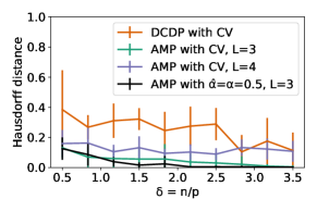
(a) Solid purple: AMP using $L=3,4$ and the optimal denoiser $f^{t}$ with the sparsity level estimated using CV.

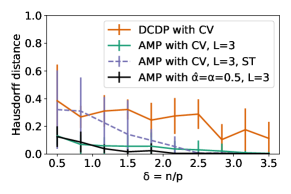
(b) Dashed purple: AMP using $L=3$ and a suboptimal soft thresholding (ST) denoiser $f^{t}$ whose threshold is selected using CV.

Figure 7: Comparison between AMP and $\mathtt{DCDP}$ in the same setting as in Figure 4: $p=200,\sigma=0.1,L^{*}=3$, sparse signal prior ${\mathbb{P}}_{\bar{\bm{B}}}=0.5{\sf N}({\bm{0}},\delta\bm{I})+0.5\delta_{{\bm{0}}}$ and AMP uses $\Delta=n/10$. Solid red: $\mathtt{DCDP}$ with hyperparameters chosen using CV. Solid green: AMP using $L=3$, the optimal denoiser $f^{t}$ with the sparsity level estimated using CV. Solid black: AMP using the true signal prior.

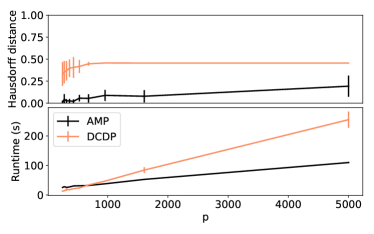
Figure 8: Comparison between AMP and $\mathtt{DCDP}$ for fixed $n=500$ and varying $p$, with $\sigma=0.1$, $L^{*}=3$ and sparse signal prior ${\mathbb{P}}_{\bar{\bm{B}}}=0.5{\sf N}({\bm{0}},\delta\bm{I})+0.5\delta_{{\bm{0}}}$. AMP uses $\Delta=n/10$ and $L=3$.

Figure 7 shows results from an additional set of experiments comparing AMP with $\mathtt{DCDP}$ (the fastest algorithm in Figure 4), using different change point priors $\pi_{\bar{{\bm{\Psi}}}}$ (Figure 7a) or denoisers $f^{t}$ (Figure 7b). In both figures, the solid red plot shows $\mathtt{DCDP}$ performance with hyperparameters chosen using CV. Solid black corresponds to AMP using the true signal prior. Solid green corresponds to AMP using $L=3$, the optimal denoiser $f^{t}$ with the sparsity level estimated using CV. In Figure 7a, AMP performs slightly worse with $L=4$ instead of $L=3$, because the prior assigns non-zero probability to the change point configurations with $L=4$ signals, which is mismatched from the ground truth $L^{*}=3$. In Figure 7b, AMP performs slightly worse at lower $\delta$ when using a suboptimal soft thresholding (ST) denoiser. Nevertheless, in both Figures 7a and 7b, AMP largely outperforms $\mathtt{DCDP}$ despite the suboptimal choices of prior or denoiser.

Figure 8 compares AMP with $\mathtt{DCDP}$ for $n=500$ and varying $p$, both using hyperparameters chosen via cross-validation. The runtime shown is the average runtime per set of CV parameters. For a fixed set of hyperparameters, the time complexity of $\mathtt{DCDP}$ scales as LASSO$(n,p)$ compared to $O(np)$ for AMP. The runtime of $\mathtt{DCDP}$ therefore grows faster with increasing $p$.

Appendix F Computational Cost

Computing $g^{*t},f^{*t+1}$

For $i\in[n]$, the function $g_{i}^{*t}$ in Proposition 3.2 only depends on $\bar{{\bm{\Psi}}}$ in (95) through the marginal probability of $\bar{\Psi}_{i}$, i.e., $\pi_{\bar{\Psi}_{i}}:\ell\mapsto\sum_{\{{\bm{\psi}}:\psi_{i}=\ell\}}\pi_{\bar{{\bm{\Psi}}}}({\bm{\psi}})$. This means $g_{i}^{*t}$ can be efficiently computed, involving only a sum over $\bar{\Psi}_{i}\in[L]$. Indeed, from the implementation details in Appendix C.2, both $f_{j}^{*t}$ and $g_{i}^{*t}$ can be computed in $O(L^{3})$ time for each $i,j$. Thus $f^{*t}$ and $g^{*t}$ can be computed in $O(nL^{3})$. The per-iteration computational cost of AMP is therefore dominated by the matrix multiplications in (LABEL:eq:amp), which are $O(npL)$.

Computing change point estimators

For estimators $\hat{{\bm{\eta}}}$ with $O(np)$ runtime, the combined AMP and estimator computation can be made to run in $O(np)$ time by selecting denoisers $f^{t},g^{t}$ as in Proposition 3.2. For example, the $\operatorname*{arg\,max}$ in (27) can be replaced with a greedy best-first search: search for the location of one change point at a time, conditioning on past estimates of the other change points. This will yield at most $L$ rounds of searching over $O(n)$ elements, resulting in $O(np)$ total runtime.

Computing the approximate posterior

For low-dimensional latent random variables ${\bm{\Psi}}$, the denominator in (30) only requires evaluating a polynomial number of terms, ${n\choose L}$ in the case of change point signal configurations. Therefore, choosing $f^{t},g^{t}$ as in Proposition 3.2, the computational complexity of computing $p_{{\bm{\Psi}}|\bar{\bm{V}}_{\bm{\Theta}}^{t},q(\bm{Z},{\bm{\Psi}},\bar{\bm{\varepsilon}})}({\bm{\psi}}|\bm{\Theta}^{t},\bm{y})$ along with AMP is $O(npL+nL^{3}+n^{L})=O(np+n^{L})$.

Appendix G Background on AMP for Generalized Linear Models (GLMs)

Here we review the AMP algorithm and its state evolution characterization for the GLM without change points. As in Section 3, let $\bm{B}\in{\mathbb{R}}^{p\times L}$ be a signal matrix and let $\bm{X}\in{\mathbb{R}}^{n\times p}$ be a design matrix . The observation $\bm{y}\in{\mathbb{R}}^{n\times L}$ is produced as

$$\bm{y}=q(\bm{X}\bm{B},\bm{\varepsilon})\in{\mathbb{R}}^{n\times L},$$ (108)

where $\bm{\varepsilon}\in{\mathbb{R}}^{n}$ is a noise vector, and $q:{\mathbb{R}}^{L}\to{\mathbb{R}}^{L}$ is a known output function. The only difference between this model and the one in (2) is the absence of the signal configuration vector ${\bm{\Psi}}$. The AMP algorithm for the GLM in (108) was derived by Rangan (2011) for the case of vector signals ($L=1$); see also Section 4 of (Feng et al., 2022). Here we discuss the algorithm for the general case ($L\geq 1$), which can be found in (Tan & Venkataramanan, 2023). For ease of exposition, we will make the following standard assumption (see (S0) on p.(S0)): as $n,p\to\infty$, the empirical distributions of $\{\bm{B}_{j}\}_{j\in[p]}$ and $\{\varepsilon_{i}\}_{i\in[n]}$ converge weakly to laws ${\mathbb{P}}_{\bar{\bm{B}}}$ and ${\mathbb{P}}_{\bar{\varepsilon}}$, respectively, with bounded second moments. We also recall that $n/p\to\delta$ as $n,p\to\infty$.

The AMP algorithm for the model (108) is the same as the one in (LABEL:eq:amp), but due to the assumption above, we can take $f^{t},g^{t}$ to be separable, i.e., $f^{t}:{\mathbb{R}}^{L}\to{\mathbb{R}}^{L}$ and $g^{t}:{\mathbb{R}}^{L}\times{\mathbb{R}}^{L}\to{\mathbb{R}}^{L}$ act row-wise on their matrix inputs. Then, the matrices $\bm{F}^{t}$ and $\bm{C}^{t}$ in (LABEL:eq:amp) can be simplified to $\bm{C}^{t}=\frac{1}{n}\sum_{i=1}^{n}\textrm{d}g^{t}(\bm{\Theta}_{i}^{t},y_{i})$ and $\bm{F}^{t}=\frac{1}{n}\sum_{j=1}^{p}\textrm{d}f^{t}(\bm{B}_{j}^{t})$, where $\textrm{d}g^{t}$ and $\textrm{d}f^{t}$ denote the $L\times L$ Jacobians with respect to the first argument.

State evolution

The memory terms $-\hat{{\bm{R}}}^{t-1}(\bm{F}^{t})^{\top}$ and $-\hat{\bm{B}}^{t}(\bm{C}^{t})^{\top}$ in (LABEL:eq:amp) debias the iterates $\bm{\Theta}^{t}$ and $\bm{B}^{t+1}$ and enable a succinct distributional characterization, guaranteeing that their empirical distributions converge to well-defined limits as $n,p\to\infty$. Specifically, Theorem 1 in (Tan & Venkataramanan, 2023) shows that for each $t\geq 1$, the empirical distribution of the rows of $\bm{B}^{t}$ converges to the law of a random vector $\tilde{\bm{V}}_{\bm{B}}^{t}:=\bar{\bm{B}}\tilde{{\bm{\nu}}}^{t}_{\bm{B}}+\tilde{\bm{G}}^{t}_{\bm{B}}\,\in{\mathbb{R}}^{1\times L}$, where $\tilde{\bm{G}}^{t+1}_{\bm{B}}\sim{\sf N}(0,\tilde{{\bm{\kappa}}}_{\bm{B}}^{t,t})$ is independent of $\bar{\bm{B}}\sim{\mathbb{P}}_{\bar{\bm{B}}}$. Similarly, recalling that $\bm{\Theta}=\bm{X}\bm{B}\in{\mathbb{R}}^{n\times L}$, the empirical distribution of the rows of $(\bm{\Theta},\,\bm{\Theta}^{t})$ converges to the law of the random vectors $(\tilde{{\bm{Z}}},\tilde{{\bm{Z}}}\tilde{{\bm{\nu}}}^{t}_{\bm{\Theta}}+\tilde{\bm{G}}^{t}_{\bm{\Theta}})$, where $\tilde{\bm{G}}^{t+1}_{\bm{\Theta}}\sim{\sf N}(0,\tilde{{\bm{\kappa}}}_{\bm{\Theta}}^{t,t})$ is independent of $\tilde{{\bm{Z}}}\sim{\sf N}\left(0,\delta({\mathop{\mathbb{E}}}[\bar{{\bm{B}}}\bar{{\bm{B}}}^{\sf T}])^{-1}\right)$. The deterministic $L\times L$ matrices $\tilde{{\bm{\nu}}}^{t}_{\bm{B}},\tilde{{\bm{\kappa}}}_{\bm{B}}^{t,t},\tilde{{\bm{\nu}}}_{\bm{\Theta}}^{t,t}$, and $\tilde{{\bm{\kappa}}}_{\bm{\Theta}}^{t,t}$ can be recursively computed for $t\geq 1$ via a state evolution recursion that depends on $f^{t},g^{t}$ and the limiting laws ${\mathbb{P}}_{\bar{\bm{B}}}$ and ${\mathbb{P}}_{\bar{\varepsilon}}$.

The state evolution characterization allows us to compute asymptotic performance measures such as the MSE of the AMP algorithm. Indeed, for each $t\geq 1$, we almost surely have $\lim_{p\to\infty}\frac{1}{p}\|f^{t}(\bm{B}^{t})-\bm{B}\|_{F}^{2}={\mathop{\mathbb{E}}}[\|f^{t}(\tilde{\bm{V}}_{\bm{B}}^{t})-\bar{\bm{B}}\|^{2}_{2}]$, where the expectation on the right can be computed using the joint law of the $L$-dimensional random vectors $\bar{\bm{B}}$ and $\tilde{\bm{V}}_{\bm{B}}^{t}=\bar{\bm{B}}\tilde{{\bm{\nu}}}^{t}_{\bm{B}}+\tilde{\bm{G}}^{t}_{\bm{B}}$.

In the model (3) with change points, we have an additional signal configuration vector ${\bm{\Psi}}$, because of which we cannot take the AMP denoising function $g^{t}$ to be separable, even under Assumption (S0). This leads to a more complicated state evolution characterization, as described in Section 3.

References

• Andreou & Ghysels (2002) Andreou, E. and Ghysels, E. Detecting multiple breaks in financial market volatility dynamics. Journal of Applied Econometrics, 2002.
• Arpino & Liu (2024) Arpino, G. and Liu, X. AMP implementation for change point inference in high-dimensional linear regression. https://github.com/gabrielarpino/AMP_chgpt_lin_reg, 2024.
• Aston & Kirch (2012) Aston, J. A. D. and Kirch, C. Evaluating stationarity via change-point alternatives with applications to fmri data. The Annals of Applied Statistics, 2012.
• Bai & Safikhani (2023) Bai, Y. and Safikhani, A. A unified framework for change point detection in high-dimensional linear models. Statistica Sinica, 2023.
• Barbier et al. (2019) Barbier, J., Krzakala, F., Macris, N., Miolane, L., and Zdeborová, L. Optimal errors and phase transitions in high-dimensional generalized linear models. Proceedings of the National Academy of Sciences, 116(12):5451–5460, 2019.
• Barbier et al. (2020) Barbier, J., Macris, N., and Rush, C. All-or-nothing statistical and computational phase transitions in sparse spiked matrix estimation. In Neural Information Processing Systems (NeurIPS), 2020.
• Bayati & Montanari (2011) Bayati, M. and Montanari, A. The dynamics of message passing on dense graphs, with applications to compressed sensing. IEEE Transactions on Information Theory, 57:764–785, 2011.
• Berthier et al. (2019) Berthier, R., Montanari, A., and Nguyen, P.-M. State evolution for approximate message passing with non-separable functions. Information and Inference: A Journal of the IMA, 2019.
• Bhattacharjee et al. (2020) Bhattacharjee, M., Banerjee, M., and Michailidis, G. Change Point Estimation in a Dynamic Stochastic Block Model. Journal of Machine Learning Research, 2020.
• Bradbury et al. (2018) Bradbury, J., Frostig, R., Hawkins, P., Johnson, M. J., Leary, C., Maclaurin, D., Necula, G., Paszke, A., VanderPlas, J., Wanderman-Milne, S., and Zhang, Q. JAX: composable transformations of Python+NumPy programs, 2018. 0.3.13.
• Braun et al. (2000) Braun, J. V., Braun, R., and Müller, H.-G. Multiple changepoint fitting via quasilikelihood, with application to dna sequence segmentation. Biometrika, 2000.
• Cho & Fryzlewicz (2015) Cho, H. and Fryzlewicz, P. Multiple-change-point detection for high dimensional time series via sparsified binary segmentation. Journal of the Royal Statistical Society Series B: Statistical Methodology, 2015.
• Cho et al. (2024) Cho, H., Kley, T., and Li, H. Detection and inference of changes in high-dimensional linear regression with non-sparse structures, 2024. arXiv:2402.06915.
• Deshpande & Montanari (2014) Deshpande, Y. and Montanari, A. Information-theoretically optimal sparse PCA. In IEEE International Symposium on Information Theory (ISIT), pp.  2197–2201, 2014.
• Donoho et al. (2009) Donoho, D. L., Maleki, A., and Montanari, A. Message passing algorithms for compressed sensing. Proceedings of the National Academy of Sciences, 106:18914–18919, 2009.
• Donoho et al. (2013) Donoho, D. L., Javanmard, A., and Montanari, A. Information-theoretically optimal compressed sensing via spatial coupling and approximate message passing. IEEE Transactions on Information Theory, 59(11):7434–7464, Nov. 2013.
• Fan & Guan (2018) Fan, Z. and Guan, L. Approximate $\ell_{0}$-penalized estimation of piecewise-constant signals on graphs. The Annals of Statistics, 46(6B):3217 – 3245, 2018.
• Fearnhead (2006) Fearnhead, P. Exact and efficient bayesian inference for multiple changepoint problems. Statistics and computing, 16:203–213, 2006.
• Feng et al. (2022) Feng, O. Y., Venkataramanan, R., Rush, C., and Samworth, R. J. A Unifying Tutorial on Approximate Message Passing. Foundations and Trends® in Machine Learning, 15(4):335–536, 2022.
• Fletcher & Rangan (2018) Fletcher, A. K. and Rangan, S. Iterative reconstruction of rank-one matrices in noise. Information and Inference: A Journal of the IMA, 7(3):531–562, 2018.
• Fryzlewicz (2014) Fryzlewicz, P. Wild binary segmentation for multiple change-point detection. The Annals of Statistics, 42(6):2243–2281, 2014.
• Gao & Wang (2022) Gao, F. and Wang, T. Sparse change detection in high-dimensional linear regression, 2022. arXiv:2208.06326.
• Gerbelot & Berthier (2023) Gerbelot, C. and Berthier, R. Graph-based approximate message passing iterations. Information and Inference: A Journal of the IMA, 2023.
• Javanmard & Montanari (2013) Javanmard, A. and Montanari, A. State evolution for general approximate message passing algorithms, with applications to spatial coupling. Information and Inference: A Journal of the IMA, 2013.
• Kabashima (2003) Kabashima, Y. A CDMA multiuser detection algorithm on the basis of belief propagation. Journal of Physics A: Mathematical and General, 36(43):11111–11121, Oct 2003.
• Kaul et al. (2019) Kaul, A., Jandhyala, V. K., and Fotopoulos, S. B. An efficient two step algorithm for high dimensional change point regression models without grid search. J. Mach. Learn. Res., 2019.
• Krzakala et al. (2012) Krzakala, F., Mézard, M., Sausset, F., Sun, Y., and Zdeborová, L. Probabilistic reconstruction in compressed sensing: algorithms, phase diagrams, and threshold achieving matrices. Journal of Statistical Mechanics: Theory and Experiment, 2012(8), 2012.
• Lavergne (2008) Lavergne, P. A Cauchy-Schwarz inequality for expectation of matrices. Discussion Papers dp08-07, Department of Economics, Simon Fraser University, November 2008.
• Lee et al. (2016) Lee, S., Seo, M. H., and Shin, Y. The Lasso for high dimensional regression with a possible change point. Journal of the Royal Statistical Society. Series B (Statistical Methodology), 2016.
• Leonardi & Bühlmann (2016) Leonardi, F. and Bühlmann, P. Computationally efficient change point detection for high-dimensional regression, 2016. arXiv:1601.03704.
• Lesieur et al. (2017) Lesieur, T., Krzakala, F., and Zdeborová, L. Constrained low-rank matrix estimation: Phase transitions, approximate message passing and applications. Journal of Statistical Mechanics: Theory and Experiment, 2017(7):073403, 2017.
• Li et al. (2023) Li, W., Wang, D., and Rinaldo, A. Divide and Conquer Dynamic Programming: An Almost Linear Time Change Point Detection Methodology in High Dimensions. In Proceedings of the 40th International Conference on Machine Learning, 2023.
• Liu et al. (2021) Liu, H., Gao, C., and Samworth, R. J. Minimax rates in sparse, high-dimensional change point detection. The Annals of Statistics, 49(2), 2021.
• Londschien et al. (2023) Londschien, M., Bühlmann, P., and Kovács, S. Random Forests for Change Point Detection. Journal of Machine Learning Research, 2023.
• Lungu et al. (2022) Lungu, V., Papageorgiou, I., and Kontoyiannis, I. Change-point detection and segmentation of discrete data using Bayesian context trees, 2022. arXiv: 2203.04341.
• Ma & Ping (2017) Ma, J. and Ping, L. Orthogonal AMP. IEEE Access, 5:2020–2033, 2017.
• Ma et al. (2019) Ma, Y., Rush, C., and Baron, D. Analysis of approximate message passing with non-separable denoisers and markov random field priors. IEEE Transactions on Information Theory, 65(11):7367–7389, 2019.
• Madrid Padilla et al. (2022) Madrid Padilla, O. H., Yu, Y., Wang, D., and Rinaldo, A. Optimal nonparametric multivariate change point detection and localization. IEEE Transactions on Information Theory, 68(3):1922–1944, 2022.
• Maillard et al. (2020) Maillard, A., Loureiro, B., Krzakala, F., and Zdeborová, L. Phase retrieval in high dimensions: Statistical and computational phase transitions. In Neural Information Processing Systems (NeurIPS), 2020.
• Metzler et al. (2016) Metzler, C. A., Maleki, A., and Baraniuk, R. G. From denoising to compressed sensing. IEEE Transactions on Information Theory, 62(9):5117–5144, 2016.
• Mondelli & Venkataramanan (2021) Mondelli, M. and Venkataramanan, R. Approximate message passing with spectral initialization for generalized linear models. International Conference on Artificial Intelligence and Statistics, pp.  397–405, 2021.
• Montanari & Venkataramanan (2021) Montanari, A. and Venkataramanan, R. Estimation of low-rank matrices via approximate message passing. Annals of Statistics, 45(1):321–345, 2021.
• Pandit et al. (2020) Pandit, P., Sahraee-Ardakan, M., Rangan, S., Schniter, P., and Fletcher, A. K. Inference with deep generative priors in high dimensions. IEEE Journal on Selected Areas in Information Theory, 1(1):336–347, 2020.
• Rangan (2011) Rangan, S. Generalized approximate message passing for estimation with random linear mixing. IEEE International Symposium on Information Theory, 2011.
• Rangan et al. (2019) Rangan, S., Schniter, P., and Fletcher, A. K. Vector approximate message passing. IEEE Transactions on Information Theory, 65(10):6664–6684, 2019.
• Rinaldo et al. (2021) Rinaldo, A., Wang, D., Wen, Q., Willett, R., and Yu, Y. Localizing Changes in High-Dimensional Regression Models. In International Conference on Artificial Intelligence and Statistics, 2021.
• Schniter & Rangan (2014) Schniter, P. and Rangan, S. Compressive phase retrieval via generalized approximate message passing. IEEE Transactions on Signal Processing, 63(4):1043–1055, 2014.
• Som & Schniter (2012) Som, S. and Schniter, P. Compressive imaging using approximate message passing and a Markov-tree prior. IEEE Transactions on Signal Processing, 60(7):3439–3448, 2012.
• Takeuchi (2020) Takeuchi, K. Rigorous dynamics of expectation-propagation-based signal recovery from unitarily invariant measurements. IEEE Transactions on Information Theory, 66(1):368–386, 2020.
• Tan & Venkataramanan (2023) Tan, N. and Venkataramanan, R. Mixed Regression via Approximate Message Passing. Journal of Machine Learning Research, 24(317):1–44, 2023.
• Wang et al. (2020) Wang, D., Yu, Y., and Rinaldo, A. Univariate mean change point detection: Penalization, CUSUM and optimality. Electronic Journal of Statistics, pp.  1917 – 1961, 2020.
• Wang et al. (2021a) Wang, D., Yu, Y., and Rinaldo, A. Optimal change point detection and localization in sparse dynamic networks. The Annals of Statistics, 2021a.
• Wang et al. (2021b) Wang, D., Yu, Y., and Rinaldo, A. Optimal covariance change point localization in high dimensions. Bernoulli, 2021b.
• Wang et al. (2021c) Wang, D., Zhao, Z., Lin, K. Z., and Willett, R. Statistically and computationally efficient change point localization in regression settings. Journal of Machine Learning Research, 22(248):1–46, 2021c.
• Wang & Samworth (2018) Wang, T. and Samworth, R. J. High Dimensional Change Point Estimation via Sparse Projection. Journal of the Royal Statistical Society Series B: Statistical Methodology, 2018.
• Wang et al. (2022) Wang, T., Zhong, X., and Fan, Z. Universality of approximate message passing algorithms and tensor networks, 2022. arXiv:2206.13037.
• Xu et al. (2022) Xu, H., Wang, D., Zhao, Z., and Yu, Y. Change point inference in high-dimensional regression models under temporal dependence, 2022. arXiv:2207.12453.
• Yi et al. (2014) Yi, X., Caramanis, C., and Sanghavi, S. Alternating minimization for mixed linear regression. International Conference on Machine Learning, pp.  613–621, 2014.
• Zhang et al. (2022) Zhang, Y., Mondelli, M., and Venkataramanan, R. Precise asymptotics for spectral methods in mixed generalized linear models, 2022. arXiv:2211.11368.
• Zhang et al. (2023) Zhang, Y., Ji, H. C., Venkataramanan, R., and Mondelli, M. Spectral estimators for structured generalized linear models via approximate message passing, 2023. arXiv:2308.14507.