Tensor models and group field theories: combinatorics, large and renormalization
Sylvain Carrozzaa,111sylvain.carrozza@u-bourgogne.fr
aInstitut de Mathématiques de Bourgogne, UMR 5584, CNRS & Université de Bourgogne, F-21000 Dijon, France.
Abstract
We provide a brief overview of tensor models and group field theories, focusing on their main common features. Both frameworks arose in the context of quantum gravity research, and can be understood as higher-dimensional generalizations of matrix models. We describe the common combinatorial structure underlying such models and review some of the key mathematical results that have been obtained in this area. Of central importance is the discovery of a new family of large expansions for random tensors. It has driven applications of tensor models to random geometry and non-perturbative local quantum field theory, and has also enabled the development of rigorous renormalization methods for group field theories and other non-local quantum field theories.
1 Introduction
With the pioneering work of t’ Hooft [1], it was recognized that a quantum field theory (QFT) of an matrix field can be formally expanded into Feynman amplitudes indexed by ribbon graphs or combinatorial maps [2]. Those two equivalent combinatorial structures formalize the notion of a graph embedded into a canonically associated surface (considered up to homeomorphism), and the genus of that surface indexes a topological large expansion in which takes the role of a formal small parameter. In addition to t’ Hooft’s original idea of using this expansion to probe the non-perturbative sector of QFT, it has found numerous applications to enumerative combinatorics, and more specifically, to two-dimensional quantum gravity [3, 4, 5, 6]. Indeed, formal matrix integrals can be used to efficiently manipulate generating functions of combinatorial maps, and asymptotic enumeration results for such objects can be inferred by studying the critical properties of the underlying matrix model [7, 8]. From a physical point of view, such a critical regime can be interpreted as defining the continuum limit of a two-dimensional random geometry [9, 10] which is equivalent to Liouville quantum gravity [11, 12].
Tensor models were first considered in the early nineties [13, 14, 15], in an attempt to establish an analogous correspondence between random tensors222By convention, we reserve the word tensor for an object with indices, to contrast with the case of vectors () and matrices (). and Euclidean quantum gravity in dimension . These early works pointed to a fertile correspondence between the Feynman expansion of such a tensor model (indexed by higher generalizations of ribbon graphs) and discrete geometries in dimension . However, no generalization of the large expansion of matrix models could be identified at the time. For a while, this hindered further progress on tensor models and their relationship to random geometry.
In the meantime was introduced the formalism of Group Field Theory (GFT) [16, 17, 18]. A GFT can be understood as an algebraically enriched tensor model which generates, via its Feynman expansion, discrete spaces weighted by lattice gauge theory amplitudes (rather than mere combinatorial factors). More precisely, it is a (perturbative) QFT of a tensor field whose indices take value into a group , and the action is chosen in such a way as to generate the amplitudes of a specific lattice gauge theory with structure group . Particularly studied types of actions are those that generating lattice gauge theory amplitudes [19, 20] and discrete quantum gravity amplitudes in holonomy-flux variables [21, 22, 23, 24]. The latter can be interpreted as giving rise to models of random geometry, in which the geometry is function of both the combinatorial structure of the lattice and its attached group-theoretic data. From a mathematical point of view, GFTs suffer from divergences which are of a similar nature as those encountered in local perturbative QFT, but owing to the non-local character of a GFT action, are beyond the scope of standard perturbative QFT theorems. Hence, for some time, it was not clear if and in which sense GFTs could be considered as mathematically well-defined perturbative QFTs.
In 2009, the formalism of colored tensor models (resp. GFTs) was introduced by Gurau [25], which eventually led to the discovery of a new large expansion [26, 27, 28]. The availability of this crucial ingredient, which generalizes the large expansion of matrix models but also differs from it in crucial respects, triggered new developments in both tensor models and GFTs. On the one hand, the large expansion has allowed to make precise statements about the relation of random tensors to random geometry (see Sec. 2.2). On the other hand, the combinatorial tools developed in the context of tensor models have enabled the proof of a series of renormalization results adapted to GFT (and other non-local QFTs), which have considerably clarified their mathematical definition (see Sec. 3.2). Finally, Gurau’s large expansion and its variants (see Sec. 2.1) were later exploited to explore the non-perturbative sector of local QFTs with internal symmetry described by tensor representations (see Sec. 2.3). See [29] for a recent review.
Our review is organized as follows. In Sec. 2, we describe Gurau’s large expansion of tensor models333Gurau’s first paper on the large expansion was aimed at both tensor models and GFTs, but further results in that direction were for the most part focused on the former. and some of its variants, together with their two main applications to date: random geometry and strongly-coupled QFT. GFTs and closely related families of non-local QFTs are the focus of Sec. 3. Regarding GFT, we restrict our attention to renormalization results since they have a strong connection to tensor models. Other aspects of GFT, which have received continued attention and led to important developments in recent years are only briefly mentioned in Sec. 3.3.
2 Tensor models
2.1 Combinatorial structure and melonic large N expansions
In its simplest incarnation, a tensor model takes as input a linear subspace of multilinear maps acting on some (real, complex or quaternionic) vector space of dimension , together with the natural group action of the appropriate unitary group (namely, , or ).444We will see shortly that it is advantageous to consider more constraining symmetries defined by a product of such unitary groups. If is a space of tensors of order , one chooses an appropriate basis and simply represents by a multidimensional array (). One can then equip with a formal measure taking the form:
| (1) |
where: is a symmetric linear operator on , and the Gaussian measure of covariance ; the (interaction part of the) action is a polynomial invariant of the tensor , which is typically expanded in terms of a basis of invariant monomials ; the coupling constants are understood as formal perturbative parameters. In all the models considered in the present section, is itself assumed to be equivariant under the group action on (see Sec. 3 for models in which this condition is relaxed). One is then interested in determining the universal properties of such an object in the asymptotic limit of large dimensionality, namely . With a few notable exceptions (e.g. [30, 31]), this question has been investigated in the sense of formal power-series in . For this reason, we will make no attempt to provide a probabilistic definition of the formal measure , and will allow ourselves to consider any kind of invariant in the action (e.g. real invariants which are unbounded from below). What makes tensor models interesting from this formal point of view is that quantities such as the free energy can be interpreted as generating functions of combinatorial objects, namely combinatorial maps and higher-dimensional generalizations thereof.
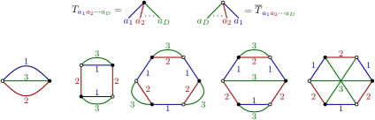
An important observation is that the space of polynomial tensor invariants is significantly richer for than it is when . To see this, it is convenient to represent tensors and their index-contractions graphically, as illustrated in Fig. 1: a tensor of order is represented by a vertex connected to half-edges, while the contraction of two indices amounts to gluing the two corresponding half-edges into an edge. Basic polynomial invariants can then be represented by closed graphs, which we illustrate in Fig. 2 for a real vector (), an Hermitian matrix (), and a completely symmetric real tensor of order (). In all three cases, a generic polynomial invariant can be decomposed as a sum of products of more basic invariants, which can be represented by connected graphs, and are thus called connected invariants. But the spaces of connected invariants are very different in each case. The vector admits a single connected invariant: the inner product , represented by a single edge.555From now on, Einstein’s convention of implicit summation over repeated indices is assumed. By contrast, the matrix admits an infinite set of connected invariants, one per order : the power sum of its eigenvalues, , which is represented by a cyclic graph with vertices. Furthermore, any two such invariants are independent in the limit . Finally, the connected invariants of a real symmetric tensor of order are in one-to-one correspondence with -regular (multi)graphs, whose number grows super-exponentially with the number of vertices (or, equivalently, the order of the invariant). Again, any two such connected invariants become independent when is sufficiently large. Such a super-exponential growth of the number of connected invariants is observed for any and for other types of tensors.666See e.g. [32, 33] for precise enumeration results. It makes the theory space of tensor models comparatively more difficult to analyze than those of vector or matrix models. However, as it turns out, the generating functions produced by specific families of tensor invariants can be of a simpler nature than those of matrix models, while remaining richer than those of vector models, which is in part what makes tensor models physically interesting.


A standard example of matrix model can be obtained by taking to be the vector space of Hermitian matrices, while setting (where is the identity map on ) and in equation (1). The primary objects of interest in such a model are expectation values of invariant observables relative to the measure , which can in principle be reconstructed from correlation functions of the form . The perturbative expansion in of such correlators can in turn be organized in terms of Feynman graphs, which in this example are -regular ribbon diagrams: they can be obtained by consistently gluing an arbitrary number of propagators and vertices with the structure shown in Fig. 3. Crucially, such ribbon diagrams can be canonically interpreted as quadrangulations of surfaces with boundaries, and the -dependence of their Feynman amplitude is entirely determined by the topology of the surface. Focusing on the free energy, which generates closed and connected quadrangulations, we obtain the celebrated topological genus expansion:
| (2) |
where is the generating function of connected quadrangulations of genus (and counts the number of quadrangles). In the asymptotic limit , such a matrix model is therefore characterized by the planar sector , and finite corrections can in principle be investigated in a perturbative expansion in . Interestingly, the structure of such an expansion allows the genus- free energy to admit better convergence properties than the full free energy, which enables a non-perturbative treatment of the coupling constant at fixed genus (and in particular in the planar sector). This was the original motivation of ’t Hooft for devising such a large expansion in the context of large gauge theory. Finally, the topological expansion (2) can be straighforwardly generalized to actions of the form , where is some (-independent) polynomial. Including a monomial proportional to in amounts to allowing ribbon vertices of degree , or dually, faces of degree in the discrete surfaces generated by the model.


A natural generalization of the previous model to the tensor realm can be obtain by letting be the space of real tensors of size (equipped with its standard inner product), and the orthogonal projector onto its symmetric subspace.777This is equivalent to taking to be the space of completely symmetric real tensors and the identity, but is somewhat more convenient for our purpose. A possible generalization of the quartic interaction we considered in the matrix case is given by the invariant represented in Fig. 4, which is often times called ’tetrahedral’ due to its combinatorial stucture (we will come back to this). This leads to the action:
| (3) |
where is the perturbative parameter and is a scaling parameter that will need to be set to an appropriate value in order to ensure the existence of a large expansion.888Note that the tetrahedral invariant is real and unbounded in both directions, contrary to the positive quartic interaction we were using in the matrix context. The model we have just defined was proposed in the very first papers on tensor models [13, 14, 15] as a way to generate, via the Feynman expansion, three-dimensional ’discrete spaces’ obtained by gluing an arbitrary numbers of tetrahedra along their faces, in analogy with matrix models. What is for sure is that the Feynman graphs of the model can be interpreted as higher generalizations of ribbon diagrams, in which through each propagator run three strands instead of two; see Fig. 4. It is however more challenging to provide a precise definition of what one would mean exactly by ’discrete space’ here. The interplay between the combinatorial structure of the action and the global structure of the Feynman diagrams, is indeed much less rigid in higher dimensions than it is in two dimensions: it is therefore challenging to ensure nice global properties (such as a manifold structure) from the Feynman rules (which only define local gluing conditions). Even more problematic, no analogue of the topological large expansion of equation (2) could be identified in this model. Progress on these questions was first achieved in the context of so-called colored tensor models, in which more constraining symmetries make the combinatorial structure of the Feynman diagrams more rigid. We now turn to a description of this important class of models, before briefly returning to real symmetric tensors at the end of the section.


An interesting structural feature of colored tensor models is their relation to the combinatorial species of edge-colored graphs. This relation was first exploited in the context of models involving a multiplet of complex tensors [25, 34, 35, 36], whose entries were labeled by an index called color. These were later subsumed by so-called uncolored models [37], which are somewhat simpler to describe in that they involve a single complex random tensor, and have as a result imposed themselves as a better starting point to develop a general theory of random tensors [38]. We will focus on this latter class of models here, which we will simply refer to as colored tensor models.999Due to later developments, the historical distinction between colored and uncolored models can be confusing.
A complex colored tensor model [38] is a theory of a complex random tensor of size , living in the -fundamental representation of . This means there is one independent unitary symmetry for each index of : for any , we have the transformation law
| (4) |
The formal measure is defined as in equation (1) with the covariance taken to be the identity, so that
| (5) |
while the action is assumed to be an invariant of the form:
| (6) |
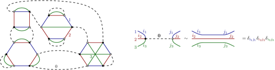
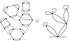
In the last formula, the sum is taken over (a finite set of) connected and bipartite -colored graphs , which index a generating set of invariants under the group action (4); see Fig. 5 for some examples. Connected -colored graphs, also known as bubbles in this context, have two types of vertices of coordination (black and white), representing a tensor or its conjugate , and types of edges labeled by an index in , called color. An edge labeled by always connects a black to a white vertex, and represents the invariant contraction of two indices in position . By a construction originally due to Pezzana which matured into a combinatorial approach to PL manifolds known as crystallization theory [39] (see also [36, 40]), any bubble diagram admits a dual interpretation as a colored triangulation of an orientable pseudomanifold101010This is a generalization of the notion of topological manifold that allows mild types of topological singularities. of dimension .111111This topological interpretation is the reason why the number of indices of a colored random tensor is denoted by the letter . For instance, the first four bubbles shown in Fig. 5 represent triangulations of the -sphere, while the fifth is dual to a triangulation of the -torus. As soon as , the colored structure of the bubbles is essential to their dual topological interpretation [34]: the color labels allow to unambiguously specify how subsimplices of arbitrary co-dimension should be identified, which is illustrated in the right panel of Fig. 6. Taking the topological cone over each such -dimensional pseudomanifold yields an elementary building block of -dimensional space (a -ball in the first four examples of Fig. 5, a pseudomanifold with a pointlike singularity in the fifth example). This construction provides a precise higher-dimensional generalization of the correspondence between matrix invariants and -gons (which is sharper, and therefore more satisfactory than what we had in the symmetric tensor model with action (3)). In the Feynman expansion, colored invariants are glued together by propagator edges, which we can assign a new color label ( by convention). With this convention in place, Feynman diagrams have the structure of -colored graphs. They are therefore dual to pseudomanifolds of dimension , which are precisely obtained by gluing together the previously mentioned topological cones along their boundaries. Having the same type of combinatorial structure encoding both tensor invariants and Feynman graphs is a remarkable property of colored tensor models. See Fig. 7 for an example of Feynman graph, and for its reinterpretation as a (colored) stranded diagram. Finally, coming back to equation (6), the parameters need to be set to appropriate values in order to ensure the existence of a large limit. This choice is not unique, but we will focus here on the so-called melonic large scaling [37], which is governed by a combinatorial quantity known as the Gurau degree [26, 27, 28, 36].
Given a connected -colored graph (e.g. a Feynman diagram), let be its number of white (resp. black) vertices and its number of faces, defined as the number of bi-colored cycles in . The Gurau degree of is a positive integer, defined by [26, 27]
| (7) |
The positivity of is not explicit in this formula, but can be recognized by re-expressing (7) as [28]
| (8) |
where runs over cyclic permutations of , is a combinatorial map canonically associated to the pair – dubbed jacket of in [41] –, and is its topological genus. The positivity of makes it an interesting higher-dimensional analogue of the standard genus of an orientable surface. This is reinforced by the realization that is nothing but the orientable genus when (which can be seen from both (7) and (8)). However, an important difference between and is that is not a topological invariant when . See [36, 38, 40] for further detail.

Now, if one sets121212A bubble being a connected -colored graph, its degree is defined by (7) after substituting for .
| (9) |
for any bubble appearing in equation (6), one can prove the existence of a sensible large expansion generalizing the one of matrix models [37]. In particular, one finds the following expression for the partition function
| (10) |
where is the generating function of connected -colored graph, enumerated by number of bubbles of each type (the variable counting the number of bubbles of type ). The leading order sector consists in connected -colored graphs of vanishing degree, which are known as melonic graphs [35]. This is the analogue of the planar sector of matrix models, and any melonic graph is indeed mapped via Pezzana’s theorem to a triangulation of the -sphere. However, since is not topological in , not every colored triangulation of the -sphere is melonic. In fact, the set of melonic graphs is quite restricted: it can be generated recursively, from the unique colored graph on two vertices, by a finite set of elementary graph insertions along edges.131313The ”melonic” qualifier is motivated by the shape of such an elementary insertion, which is reminiscent of a cataloupe melon; see Fig. 8. Melonic graphs are therefore in bijection with combinatorial trees (more specifically -ary trees). This will become important when we discuss applications of melonic large expansions.

Other large limits dominated by families of melonic diagrams (as we will see, with slightly different combinatorial properties) have been obtained in closely related tensor models. These include the original colored tensor model, built from a -tuple of complex tensors [26, 27, 28]. In the context of models involving a single tensor, there is some freedom in the choice of symmetry group, while preserving the colored structure of the Feynman graphs. Early on, the so-called multi-orientable tensor model [42, 43, 44, 45, 46], involving a complex -tensor, was shown to admit a melonic limit with an action proportional to a ’tetrahedral’ interaction of the form (note the similarity with (3)). The invariance of this model paved the way to a more systematic exploration of real colored tensor models obeying invariance. The case was first considered in [47] (with the first two interactions shown in Fig. 10), and later generalized to higher in [48]. At the combinatorial level, the main difference between real and complex colored models is that real invariants (resp. real Feynman diagrams) are labeled by connected -colored graphs (resp. -colored graphs) with no bipartite restriction imposed; see Fig. 10 for some examples. In particular, for , the action (3) obeys the desired symmetry and can rightly be represented as a non-bipartite -colored graph ( in Fig. 10). The latter can be interpretated under Pezzana’s duality as a triangulation of a non-orientable pseudomanifold.141414More precisely, it has the topology of the real projective plane. From this point of view, it is therefore somewhat misleading to call it ’tetrahedral’, which explains our use of quotation marks. Focusing on the model with interaction (3) for simplicity, one can prove that, with the large scaling defined by setting , a large expansion exists. In particular, the partition function expands as [47, 49]
| (11) |
where is a combinatorial quantity associated to Feynman graphs – again called degree –, and is the generating function of connected -colored graphs with degree . The degree of a graph is defined as (which agrees with (7)), and can again be re-expressed as a sum of genera of ribbon graphs canonically associated to . However, owing to the absence of bipartite structure in the Feynman graphs, those ribbon graphs do not need to be orientable, which explains why is in general a positive half-integer. As in complex models, leading order Feynman graphs () have a melonic structure, albeit of a slightly different type: from the point of view of the Feynman expansion, a melonic insertion has a bilocal structure, while melonic decorations where always local (that is, tadpole-like) in complex models. This difference is illustrated in Fig. 8. Generalizing this construction to arbitrary is not that straightforward, but interactions supporting a ’bilocal’ melonic large expansion have been identified for any prime in [48, 50]: they are associated to certain complete colored graphs (the ’tetrahedral’ interaction being itself represented by a complete graph on four vertices), and the somewhat surprising prime condition on is the result of combinatorial constraints that need to be imposed on the colorings of such complete graphs.
Finally, colored tensor models with more than one asymptotic parameter have been discussed in the literature. For instance, reference [51] introduced a -index random tensor obeying ,151515 here has nothing to do with the number of indices of the tensor. which can be analyzed in a double asymptotic expansion in the (formally) small parameters and . This model can equivalently be understood as a colored multi-matrix model involving a large number () of matrices. The so-called large expansion of this model [51, 52] was extended to higher order tensors in [48], and a double-scaling limit in which is kept fixed was studied in [53, 54, 55]. An interesting aspect of these models is that they allow to embed a tensor-like melonic expansion of the form (11) into the more standard genus expansion of a matrix model.
Finally, we briefly come back to the model described around equation (3), whose symmetry was described by a single copy of acting on a completely symmetric real tensor. This early proposal received renewed attention after it was convincingly argued in [56] that it should support a (bilocal) melonic large expansion if the random tensor is not only taken to be symmetric, but also traceless. This crucial observation, supported by explicit empirical checks, was proven rigorously in [57] (see also [58]), then generalized to the other two irreducible -tensor representations of [57, 59]. These results were then extended to -index irreducible tensors () [60], which suggests that bilocal melonic limits might exist for arbitrary (or, at the very least, prime ). Similar techniques have allowed to partially extend the results of [51] about the large expansion of colored matrix models to Hermitian matrices [61]. In all those works (and particularly so in [57] and [60]), the absence of colored structure makes the combinatorial proofs traditionally employed in the analysis of tensor models rather involved. This calls for the development of alternative methods, which might be better suited to the analysis of irreducible random tensors. Finally, tensor models with symplectic symmetry have been considered in [62] () and [63, 64] ().
2.2 Random geometry
It was realized in the 70s and 80s that matrix models can be used to model continuum random surfaces, or 2d Euclidean quantum gravity [3, 4, 5, 6]. In a first step, the topological large expansion is used to generate an ensemble of random discretizations of two-dimensional orientable surfaces as in (2). Taking the strict limit of this partition function (appropriately rescaled by ) produces a generating function of discretizations of the -sphere. Each such discretization can be endowed with a natural metric,161616For instance, one can attribute the same flat reference metric to all building blocks, and in this way endow the surface with a piecewise flat metric. In the dual ribbon graph representation, one may instead rely on the graph distance. so one can think of the matrix model as producing a random discrete metric space. A (somewhat heuristic) continuum limit can then be obtained by tuning to the (real, positive) critical value of .171717This makes sense because indeed has a finite radius of convergence, even though the full partition function one started from had vanishing radius of convergence. The basic idea is that, as the sum over surfaces becomes dominated by discrete geometries involving an arbitrarily large number of elementary building blocks. The upshot is that the critical regime of matrix integrals in the limit may be thought of as encoding continuum random surfaces of genus .181818As a side note, a non-trivial sum over topology can be recovered by performing a so-called double-scaling limit, in which the and limits are performed jointly while keeping the quantity fixed, for some appropriate . The probabilistic object behind this limit, known as the Brownian map [9, 10], has been constructed rigorously as the limit of various families of uniform random planar maps with fixed number of vertices.191919Each map is equipped with the graph distance, suitably rescaled by in the limit. The result is a random metric space which is (almost surely) homeomorphic to a -sphere, has spectral dimension and Hausdorff dimension .202020Convergence is defined in the sense of Gromov-Hausdorff in the space of all compact metric spaces. Furthermore, the limit is universal in the sense that it is largely independent of the details of the combinatorial maps being considered (which in the matrix model picture, is related to the choice of potential), and it is furthermore equivalent to Liouville quantum gravity [11, 12].
Random tensor models were initially motivated by the challenge of generalizing the success story of matrix models to Euclidean quantum gravity in dimension. Of all attempts made until now, the framework of complex colored tensor models seems to be the soundest from a topological point of view, thanks to its connection to colored diagrams, which can be rigorously interpreted as higher-dimensional discretized (pseudo)manifolds.212121In , it was proven that uniform colored triangulations of the -sphere do converge to the Brownian map [65], so we have no a priori reason to reject colored triangulations as an insufficiently general combinatorial structure to explore random geometry in . Moreover, the large limit of (10) generates an ensemble of colored triangulations of the -sphere, as was the case in . The main difference is that these are limited to melonic triangulations, which constitute a quite restricted set of triangulated spheres. The fact that they are in bijection with trees actually leads to a rather simple behaviour as compared to what is found in matrix models. For instance, the generating function of rooted melonic -colored triangulations, which governs the genus- sector of the original colored tensor model (as well as an ’uncolored’ version (6) in which an infinite set of bubble interactions have been switched on [37]), obeys the simple polynomial equation:
| (12) |
which one may recognize as the equation for the generating function of Fuss-Catalan numbers. The critical properties of , as well as the asymptotic enumeration of (rooted) melonic -colored triangulations, can readily be extracted from this equation [35], leading to
| (13) |
The square-root singularity of and the exponent in the second relation are directly related [66],222222By contrast, the number of rooted planar maps with vertices scales asymptotically with an exponent , which is typical of planar combinatorial objects. and indicative of a continuum limit governed by Aldous’ continuous random tree [67, 68] (also known as the branched polymer phase in the physics literature [69, 70]). This is a random metric space of non-integer spectral dimension (and Hausdorff dimension ), which can be obtained as a scaling limit of uniform random trees of size (equipped with the graph distance multiplied by a corrective factor ). It was confirmed in [71] that uniform melonic triangulations of size similarly converge to Aldous’ continuum random tree, for any topological dimension . This is a somewhat disappointing but rather remarkable universality result: while tensor models in the melonic scaling (9) offer an interesting generalization of the topological large expansion of matrix models, unlike the latter, the random geometries they generate tend to degenerate into tree-like metric spaces in the continuum limit. More generally, it is reasonable to expect that the same result should hold for any other model exhibiting a large limit dominated by tree-like combinatorial species. Henceforth, a number of attempts have been made to evade such tree-like combinatorial behaviour, which we now briefly describe.
First, double-scaling limits in which the large and critical limits are taken simultaneously have been constructed [72, 73, 74], with the idea that incorporating subleading contributions of tensor models into the continuum limit might be sufficient to change its universality class. However, the structure of fixed-degree Feynman graph, as unraveled in the complex colored setting in [75], seems to invalidate this strategy for the standard melonic scaling of (9): for any , there is only a finite number of connected Feynman graphs of degree modulo insertions of melonic two-point subgraphs and ladder four-point subgraphs (such equivalent classes of graphs are known as schemes). Given that the generating function of ladder diagrams can be resummed explicitly as a geometric series (see Fig. 9), there seems to be no room to evade the universality class of branched polymers. Furthermore, similar results have been obtained within alternative melonic large expansions, such as e.g. the model [45, 76, 77, 78, 79].
However, as argued in Sec. 2.1, the theory space of tensor models is much vaster than that of matrix models. In particular, other scalings than the melonic one can be considered to obtain alternative but consistent large limits.232323In fact, due to the proliferation of invariants with arbtrarily complex combinatorial structures, determining the optimal scaling of a bubble (i.e. the smallest value of in (10) compatible with the existence of a large expansion) is a challenging question in general. See [40] and references therein for further detail. For instance, it is straightforward to emulate matrix-like large limits in the context of a tensor model with even [80], which demonstrates that the Brownian map universality class can be obtained within tensor models. More complicated examples of non-melonic large limits have been constructed in [80, 81, 82, 40], but all of them lead to a critical regime which is either tree-like or planar-like, or that mixes tree-like and planar-like structures. In , a theorem due to Bonzom [83] indicates that any reasonable bubble interaction (that is, a -colored graph of genus , representing the triangulated boundary of a -ball) will lead to the universality class of branched polymers.
Further strategies might be considered. For instance, if one attempts to generate random geometries from other tensor model observables than the generating function of connected Feynman graphs, the universality class of the continuum limit might change. Indeed, it was observed in the colored multi-matrix model of [53] (considered in some triple-scaling limit) that restricting the sum over graphs to -particle irreducible (or, equivalently, -edge connected) contributions was sufficient to turn a melonic critical regime into a model of random maps coupled to the Ising model. Whether such a combinatorial mechanism might prove useful to generate a higher-dimensional random geometry from random tensors remains to be explored.
For now, getting out of the universality classes of continuous random trees and random maps remains a challenge for tensor models. More broadly, obtaining a non-trivial random metric space with integer spectral dimension as a scaling limit of discrete geometries is an outstanding open question for any approach; see e.g. the extensive literature on (causal) dynamical triangulations ([84] and references therein), or [85, 86] for more specific proposals aiming at overcoming this roadblock.
2.3 Large N (local) quantum field theory
What limits the scope of melonic large limits in the purely combinatorial context of random geometry (a universal tree-like behaviour at criticality) makes them quite useful in the context of large quantum mechanics and QFT. More precisely, the bilocal melonic limits described in Sec. 2.1 have been taken advantage of to explore the strong coupling regime of Q(F)T by means of analytical methods [87, 88, 89, 90], a feat which is typically out of reach even at large (at least in the absence of additional structures, such as integrable ones).
It was first realized by Witten [91], then by Klebanov and Tarnopolsky [92], that tensor models are able to emulate the physics of the Sachdev-Ye-Kitaev model [93, 94, 95]. The latter describes a disordered quantum-mechanical system of Majorana fermions (), with all-to-all interaction Hamiltonian . Taking the random couplings to be independent centered Gaussian variables with leads to a consistent large limit (for the quenched theory). If one takes in addition the strong coupling limit , an emergent time-reparametrization symmetry makes the model explicitly solvable. This symmetry and the way in which it is (spontaneously and explicitly) broken, leading to an effective Schwarzian dynamics [95, 96], is structurally identical to what is found in a two-dimensional model of gravity known as Jackiw-Teitelboim gravity [97]. As first described by Kitaev [94], this observation leads to a rather explicit holographic duality between SYK-like quantum mechanics and quantum gravity, which has received a lot of attention in recent years, notably for its applications to the theory of quantum chaos and quantum black holes (see e.g. the review [98]). Interestingly for us here, a key property of the SYK model is that its large limit is dominated by melonic Feynman diagrams (see e.g. [99]), which can be explicitly resummed in the strong coupling regime. To be more precise, this melonic limit is of a bilocal type, which turns out to be essential to generate the interesting physics we just hinted at. The pioneering works of Witten and Klebanov-Tarnopolsky recognized that the bilocal melonic limits of tensor models can also support SYK-like physics, with the advantage that no disorder needs to be introduced. Witten’s model [91] was formulated in the original colored framework proposed by Gurau [26], while the Klebanov-Tarnopolsky model [92] relied on the ’uncolored’ combinatorial structure of the model [47]. Since the latter has imposed itself as the large structure of choice in later works, we focus on the Klebanov-Tarnopolsky model here. It describes Majorana fermions (), with action
| (14) |
Note that the interaction part of the action is given by a ’tetrahedral’ invariant as in (3) (corresponding to the colored bubble of Fig. 10), the main difference being the non-trivial time-dependence. We have in particular a non-trivial propagator, and a deterministic interaction which is local in time. The structure of the large limit is identical to the one described in (11), except that the Feynman amplitudes and fixed-degree partition functions are more complicated. In particular, in the we have a closed equation for the full two-point function [92, 94, 95]
| (15) |
where and denotes the same quantity at . This equation is structurally similar to (12), and actually results from the same melonic Schwinger-Dyson equation, as represented in Fig. 9. In the strong-coupling regime , the second term on the right-hand side can be shown to dominate over the first one [94, 95], which leads to the simplified equation
| (16) |
Remarkably, this equation is invariant under reparametrizations of time
| (17) |
and admits a conformal solution of conformal dimension . This solution spontaneously breaks the reparametrization symmetry down to , leading to Goldstone modes .242424We are assuming an topology for the (Euclidean) time direction, which is appropriate for a thermal path-integral. The effective dynamics of can in turn be determined by analysing the explicit breaking of the reparametrization symmetry introduced by in (17). This can be done analytically thanks to another structurally important feature of bilocal melonic large expansions: their leading order four-point functions can be resummed explicitly as geometric series of ladder diagrams. This allows to compute the leading inverse coupling correction to the conformal dynamics, which leads to an effective dynamics for the Goldstone modes governed by the so-called Schwarzian action
| (18) |
The observation that the same Schwarzian dynamics governs boundary modes of Jackiw-Teitelboim gravity on the hyperbolic disk [97], has led to the development of the much studied holographic correspondence between SYK-like many-body models and quantum gravity on [98].
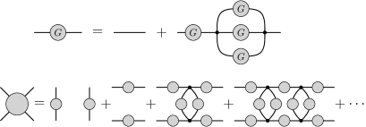
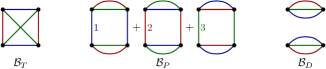
An interesting feature of the Klebanov-Tarnopolsky model of (14) over the standard SYK model is that it naturally fits in the framework of local QFT, and can in particular be generalized to higher spacetime dimensions. This has been taken advantage of in recent years to construct a new family of large QFTs [88, 89, 90] which enjoy similarly nice analytical properties as the SYK model: namely, the full two-point function obeys a closed Schwinger-Dyson equation at leading order, while information about four-point functions (as well as higher-point correlators) can be recovered from a resummation of certain classes of ladder diagrams; see Fig. 9. In particular, one can consider a real bosonic tensor field in spacetime dimensions, with -invariant (and color symmetric) action
| (19) | ||||
where , and are the quartic invariants represented in Fig. 10, and is some fixed parameter. is nothing but the ’tetrahedral’ interaction, while (’pillow’) and (’double-trace’) need to be included for consistency of the renormalization group flow. This class of models was first considered in [100] with the standard propagator (that is, setting in (19)) and in . It was shown that, at leading order in and , the -functions of the model admit a non-trivial fixed point with , and all real of order . This defines an infrared conformal field theory, which is however unstable due to the presence of an operator of complex dimension [100, 101]. This instability motivated a modification of the model [102] in which: 1) the propagator is taken to be long-range, meaning that in (19); 2) the ’tetrahedral’ coupling is assumed to be purely imaginary. More precisely, setting makes the quartic interaction marginal, and as a consequence of the long-range propagator, there is no wave-function renormalization. This simplification, together with the melonic structure, allows to compute flow equations non-perturbatively in the coupling constants, and to construct explicit renormalization group trajectories that flow to a unitary CFT in the IR [103, 104, 105]. This result provides a well-controlled mathematical framework in which to test key paradigms of QFT: for instance, it was proven that the long-range model in obeys the -theorem [106]. Finally, the model (19) with purely imaginary ’tetrahedral’ coupling constant was also considered for (short-range) and , where it was observed that the -functions are consistent with a well-behaved and asymptotically free theory in the ultraviolet [107]. Further results on tensor quantum mechanics and tensor QFT can be found in e.g. [108, 109, 110, 111, 112, 113, 114, 115, 116, 117, 118, 119, 120, 121, 122, 123, 124, 125].
3 Group field theories
3.1 Nonlocal field theories of a tensorial type
The framework of GFT [16, 17, 18] can be understood as a further generalization of tensor models, in which tensor ’indices’ are taken to live in a Lie group , which we will assume to be compact. This extra group structure can be exploited to equip the stranded graphs of tensor models with lattice gauge theory data, and weigh their amplitudes accordingly. In a similar way as the Feynman expansion of a tensor model can be interpreted as generating a random (discrete) geometry, the Feynman expansion of a GFT can be understood as defining a lattice gauge theory on a random lattice. Prototypical examples are provided by the Boulatov and Ooguri models [19, 20]. They are theories of a single field obeying the so-called gauge invariance condition (or closure constraint):
| (20) |
In the template of equation (1), this condition can be imposed by choosing to be the orthogonal projector on field configurations obeying the closure constraint, whose integral kernel is:
| (21) |
and in this formula can ultimately be interpreted, on a given Feynman graph, as parallel transport between two interaction vertices connected by a propagator line. The interaction originally considered by Boulatov [19], with and , was a ’tetrahedral’ interaction analogous to (3),252525The Ooguri model is similarly defined in , with an interaction following the combinatorial pattern of a -simplex. or in its colored version
| (22) |
Complex variants of this model, based on bipartite colored bubble interactions, started to be considered in the original papers on melonic large expansions [25, 26], and made the structure of the random lattice better defined from a topological standpoint [34, 36]. In this framework, the Boulatov model generates lattice gauge theory amplitudes which are topological invariants (modulo divergences that need to be regularized in an appropriate way). In the special case , those can be interpreted as three-dimensional Euclidean quantum gravity path-integrals expressed in holonomy-flux variables, and are mapped upon Fourier transform to the Ponzano-Regge state-sum model [126]. This correspondence between the Boulatov and Ponzano-Regge models has motivated numerous further works exploring the relation between GFT and quantum gravity, and more specifically so in the context of loop quantum gravity and spin foam models [21, 22, 127, 128, 129, 23, 24, 130, 131].262626This is where the term group field theory actually originates from. From this perspective, GFT provides a tentative albeit natural completion of spin foam models,272727See [132] for an alternative approach. one that enables the use of standard QFT concepts and methods (e.g. renormalization) to explore their phase structure. The most studied spin foam models of four-dimensional quantum gravity (see e.g. [133, 134] for reviews), which share certain features of the simpler models we will restrict our attention to, can all be embedded into the GFT framework.
The GFT formalism aims at defining QFTs of spacetime, rather than on spacetime. It is therefore not constrained by the same notion of (spacetime) locality that is so fundamental in standard QFT. Indeed, from a mathematical standpoint, a GFT can be understood as a non-local QFT on the manifold , in which interactions obey a particular kind of non-locality (sometimes referred to as combinatorial non-locality): for instance, the interaction (22) involves an integration on , which makes it non-local, but it has a rather specific structure in which individual group elements in interact locally by pairs. This pairwise locality is the essence of GFT; it constrains the kind of interactions one can legitimately consider in a similar way as the ordinary notion of spacetime locality does in standard QFT.
Like any other QFT, a GFT is typically plagued with divergences which arise from the short scale structure of the configuration space . These must be regularized and renormalized away in some consistent manner. Two approaches have been considered to achieve this goal. In the first, one looks for an asymptotic large expansion analogous to the ones described in Sec. 2 for purely combinatorial models, where is identified to a cut-off within a suitable regularization scheme. For instance, one may consider a regularized version of the propagator (21)
| (23) |
where is the heat-kernel at time on , which imposes a smooth cut-off of order on dimensions of irreducible representations labelling harmonic modes.282828E.g. when , we have (24) where is the character of the spin- irreducible representation of . This has the effect of regularizing any possible divergence of models of the Boulatov-Ooguri type, and one may then investigate which asymptotic scalings of their bubble interactions lead to consistent large limits. After pioneering steps were made in this direction [135, 136, 41, 127, 137, 138, 139], the first large results of Gurau opened the way to a thorough investigation of complex and colored versions of the Boulatov-Ooguri models, which were found to obey a consistent large expansion dominated by melonic diagrams [26, 27, 28, 140, 141, 142]. The critical properties of the leading-order sector have also been analyzed in some respects [143], but remain significantly less understood than for colored tensor models. In particular, the natural metric interpretation of GFT Feynman graphs is function of their combinatorial structure, but also of the group data attached to their edges. This makes a precise analysis of GFT models of random geometry difficult. To our knowledge, no definitive results have been obtain regarding the metric properties of their continuum limit.
The second approach to a rigorous definition of GFTs embraces their interpretation as QFTs, and looks for an appropriate generalization of the full machinery of (perturbative and non-perturbative) renormalization. An important challenge is that no a priori notion of spacetime scale is available in GFT, and neither is the usual notion of locality, so it is not immediately clear what one would even mean by a flow of local interactions parametrized by a scale. This problem was first addressed and resolved in the context of GFTs in which no gauge invariance condition has been imposed, which are known in the literature as (tensor or) tensorial field theories [144, 145, 146] (not to be confused with the local field theories of Sec. 2.3!). Such models do not exploit the group structure to produce a sum over lattice gauge theory or quantum gravity amplitudes, and have in particular no direct connection to spin foams, but they remain mathematically interesting in their own right.
3.2 Renormalization
In standard QFT, the renormalization group method relies on an harmonious interplay between spacetime scales and locality, in the sense that high energy radiative corrections to local interactions remain local as seen from low energy. In tensorial field theories, it was proposed that colored tensorial invariance should play the role of locality, meaning that, in complete analogy with tensor models, basic interactions should be labeled by connected colored graphs encoding pairwise convolutions of the group variables of the field. In an ordinary QFT, the energy scale ladder can be put in correspondence with the non-trivial spectrum of the propagator. In the GFT context, this motivates the introduction of a more abstract notion of scale, defined as an element of the spectrum of the propagator. Obviously, such a definition is relevant only in situations when the propagator has a rich spectrum, which is not the case of e.g. the Boulatov-Ooguri propagator (21) (since it is a projector). This observation, together with other arguments [147], motivated the introduction of tensorial field theories and GFTs with non-trivial propagators (such as e.g. where is the Laplace-Beltrami operator on ).
This strategy was first proposed in the pioneering work [144], where it was proven that the abstract notions of locality and scale thus defined can support a consistent perturbative renormalization scheme for tensorial field theories. Moreover, a first all-order perturbative renormalizability theorem was obtained by means of rigorous multiscale renormalization methods [148]. Further results of this kind were obtained in subsequent works, such as [146, 149, 150, 151, 152, 153]. Interestingly, there is a close analogy between the perturbative renormalization analysis of tensorial field theories and the large analysis of tensor models. The superficial degree of divergence of a Feynman graph can be expressed in terms of Gurau’s degree (7), while scaling dimensions of perturbative coupling constants are analogous to the scaling parameters from (6). It is also crucial in the renormalization analysis that divergent graphs tend to have a simple combinatorial structure (such as a melonic one). Hence, from a qualitative point of view, it is possible to interpret the renormalization group flow of a tensorial field theory as dynamically generating a consistent asymptotic large scaling, similar to those that are being imposed by hand in the tensor model setting.
The perturbative renormalization analysis of tensorial field theories was generalized in [154, 155, 156, 157] to GFT proper, that is to say to tensor field theories with gauge invariance condition (20). To be more precise, the class of GFT models considered in those works are complex models with regularized propagator292929This is a regularized version of , in which the eigenvalues of of order or larger have been smoothly cut-off.
| (25) |
and interactions labelled by connected -colored diagrams. The superficial degree of divergence of a Feynman graph has been determined to be of the form [156]
| (26) |
where is the number of propagator lines of , its number of bi-colored cycles involving the color (or faces), is the rank of the adjacency matrix between its lines and faces, and the dimension of . Divergences arise from subgraphs with , and formula (26) can be exploited to classify the set of potentially renormalizable models in terms of the free parameters , , as well as the list of bubble interactions included in the action [156, 158]. And just like for models with no gauge invariance, the multiscale renormalization methods of [148] turn out to be well-suited to the proof of all-order perturbative renormalizability theorems, because they allow to efficiently deal with the renormalization of overlapping divergent subgraphs. In particular, it was shown that with and , the sextic model involving the first four interactions shown in Fig. 5 is perturbatively renormalizable at all orders [156], and its discrete multiscale flow equations were analyzed in detail in [159]. The fact that ultraviolet divergences can be reabsorbed into effective interactions which still obey the criterion of tensorial locality is non-trivial in this model; it relies on a nice interplay between the topology of the Feynman graphs (as defined via Pezzana’s duality) and the lattice gauge theory structure of their amplitudes. We refer to the review [158] and references therein for more details on this class of models.
Other interesting results have been obtained about the renormalization of tensorial field theories and GFTs. To begin with, it was established in [149] that tensor field theories can generate renormalization group flows which are asymptotically free in the utraviolet. This may appear surprising given their superficial similarity to standard scalar field theories (which are not compatible with asymptotic freedom), but it turns out to be a consequence of the non-trivial combinatorial structure of tensorial interactions. In [160], it was shown that wave-function renormalization tends to dominate over vertex renormalization, and that, as a result, asymptotic freedom is a robust feature of quartic models. The situation is more complicated in models involving marginal interactions of higher order, as exemplified by the sextic model of [156], which fails to be asymptotically free for somewhat subtle reasons [160]. Nonetheless, it became clear from these results that tensor field theory provides non-trivial examples of QFTs which are mathematically interesting in their own right, independently from their eventual relation to GFT or quantum gravity. Since then, tensor field theory has been used as a test bed for constructive renormalization programs: for instance, the multiscale renormalization methods of [148, 161, 162] have been employed to construct renormalizable tensorial field theories in [163, 164, 165], and more recently, such models were revisited through the lenses of stochastic analysis [166]. In another direction, the perturbative renormalization struture underlying tensor field theories was shown to fit in the general Hopf-algebraic framework due to Connes and Kreimer [167, 168, 169, 170]. Finally, a number of efforts have been made to map out the non-perturbative fixed points of tensor field theories and GFTs by means of Functional Renormalization Group (FRG) methods. This program started out with the analysis of [171, 172], which focused on models without gauge invariance condition, and was then applied to proper GFTs in [173, 174, 175, 176, 177, 178]. As far as quantum gravity is concerned, it is hoped that non-perturbative FRG methods in appropriate truncations will help map out the phase diagrams of GFTs in the infrared regime, and eventually allow to locate non-perturbative fixed points which have the potential to lead to interesting continuum limits. We refer to the recent literature [179, 180, 181, 182] for a detailed account and status of this search (see also [183, 184] for applications of functional renormalization to the search of consistent large limits).
We conclude this section with two open questions regarding the renormalization of GFTs. First, while rigorous perturbative renormalization theorems are already available for simple classes of GFTs (tensor field theories, and GFTs resembling the Boulatov-Ooguri models), can those results and the methods they rest on be extended to four-dimensional quantum gravity proposals (e.g. of the type [23, 24, 130, 185, 131])? Second, how could one go about proving the existence of the non-perturbative fixed points which are empirically observed in truncated FRGs?
3.3 Further developments
We conclude by listing some important research directions on GFT which we could not give justice to in this short review.
In recent years, there has been a strong push towards applications of the GFT formalism to cosmology, and other symmetry-reduced regimes of general relativity. A mechanism of Bose-Einstein condensation adapted to GFT was investigated and argued to predict effective Friedmann equations from full-fledged quantum gravity [186, 187, 188]. A similar construction was also applied to black holes in [189, 190]. This approach is grounded in the Fock space formalism of [130]; it allows to extract a low energy effective dynamics from GFT by means of well-established methods originating from standard quantum many-body physics. We refer to the reviews [191, 192, 193] for more complete accounts of GFT cosmology.
The same many-body physics interpretation has also allowed to analyze GFT wave-functions through the lenses of entanglement theory. In particular, holographic entanglement area laws [194, 195, 196] have been derived in GFT, thus establishing interesting connections with holographic tensor networks [197, 198].
While the GFTs we focused on in the previous two subsections assumed a compact Lie group , GFT models of Lorentzian quantum gravity typically require to be non-compact (see e.g. [199, 131]). From the point of view of renormalization, this leads to an additional infrared problem, which was approached by means of FRG methods in [172, 175]. Interestingly, in recent works [200, 201], the non-compact nature of was taken advantage of to develop new mean-field approximations, which provide useful information about those models while a complete renormalization group treatment awaits.
Finally, we note that a certain type of effective melonic quantum dynamics was recently suggested to arise from a generalized Boulatov model [202]. This may lead to interesting new connections between GFT and the large QFT framework described in Sec. 2.3, which are a priori quite different (both in intent and content).
Acknowledgements
I would like to thank Razvan Gurau, Daniele Oriti and Vincent Rivasseau for their pioneering works, their contagious enthusiasm for this subject, and for teaching me much about it in the first place.
The IMB receives support from the EIPHI Graduate School (contract ANR-17-EURE-0002).
References
- [1] G. ’t Hooft, A Planar Diagram Theory for Strong Interactions, Nucl. Phys. B 72 (1974) 461.
- [2] S. K. Lando, A. K. Zvonkin and D. B. Zagier, Graphs on surfaces and their applications, vol. 141. Springer, 2004.
- [3] E. Brezin, C. Itzykson, G. Parisi and J. B. Zuber, Planar Diagrams, Commun. Math. Phys. 59 (1978) 35.
- [4] F. David, Planar Diagrams, Two-Dimensional Lattice Gravity and Surface Models, Nucl. Phys. B 257 (1985) 45.
- [5] J. Ambjorn, B. Durhuus and J. Frohlich, Diseases of Triangulated Random Surface Models, and Possible Cures, Nucl. Phys. B 257 (1985) 433.
- [6] P. Di Francesco, P. H. Ginsparg and J. Zinn-Justin, 2-D Gravity and random matrices, Phys. Rept. 254 (1995) 1 [hep-th/9306153].
- [7] B. Eynard, T. Kimura and S. Ribault, Random matrices, 1510.04430.
- [8] B. Eynard, Counting Surfaces, vol. 70 of Progress in Mathematical Physics. Springer, 2016, 10.1007/978-3-7643-8797-6.
- [9] J.-F. Le Gall, Uniqueness and universality of the brownian map, The Annals of Probability 41 (2013) 2880.
- [10] G. Miermont, The brownian map is the scaling limit of uniform random plane quadrangulations, Acta Math 210 (2013) 319.
- [11] J. Miller and S. Sheffield, Liouville quantum gravity and the brownian map i: The qle (8/3, 0) metric, arXiv preprint arXiv:1507.00719 (2015) .
- [12] E. Gwynne, Random surfaces and liouville quantum gravity, Notices of the American Mathematical Society 67 (2020) 484.
- [13] J. Ambjorn, B. Durhuus and T. Jonsson, Three-dimensional simplicial quantum gravity and generalized matrix models, Mod. Phys. Lett. A 6 (1991) 1133.
- [14] N. Sasakura, Tensor model for gravity and orientability of manifold, Mod. Phys. Lett. A 6 (1991) 2613.
- [15] M. Gross, Tensor models and simplicial quantum gravity in 2-D, Nucl. Phys. B Proc. Suppl. 25 (1992) 144.
- [16] D. Oriti, The Group field theory approach to quantum gravity, gr-qc/0607032.
- [17] L. Freidel, Group field theory: An Overview, Int. J. Theor. Phys. 44 (2005) 1769 [hep-th/0505016].
- [18] T. Krajewski, Group field theories, PoS QGQGS2011 (2011) 005 [1210.6257].
- [19] D. V. Boulatov, A Model of three-dimensional lattice gravity, Mod. Phys. Lett. A 7 (1992) 1629 [hep-th/9202074].
- [20] H. Ooguri, Topological lattice models in four-dimensions, Mod. Phys. Lett. A 7 (1992) 2799 [hep-th/9205090].
- [21] R. De Pietri, L. Freidel, K. Krasnov and C. Rovelli, Barrett-Crane model from a Boulatov-Ooguri field theory over a homogeneous space, Nucl. Phys. B 574 (2000) 785 [hep-th/9907154].
- [22] M. P. Reisenberger and C. Rovelli, Space-time as a Feynman diagram: The Connection formulation, Class. Quant. Grav. 18 (2001) 121 [gr-qc/0002095].
- [23] A. Baratin and D. Oriti, Group field theory and simplicial gravity path integrals: A model for Holst-Plebanski gravity, Phys. Rev. D 85 (2012) 044003 [1111.5842].
- [24] A. Baratin and D. Oriti, Quantum simplicial geometry in the group field theory formalism: reconsidering the Barrett-Crane model, New J. Phys. 13 (2011) 125011 [1108.1178].
- [25] R. Gurau, Colored Group Field Theory, Commun. Math. Phys. 304 (2011) 69 [0907.2582].
- [26] R. Gurau, The 1/N expansion of colored tensor models, Annales Henri Poincare 12 (2011) 829 [1011.2726].
- [27] R. Gurau and V. Rivasseau, The 1/N expansion of colored tensor models in arbitrary dimension, EPL 95 (2011) 50004 [1101.4182].
- [28] R. Gurau, The complete 1/N expansion of colored tensor models in arbitrary dimension, Annales Henri Poincare 13 (2012) 399 [1102.5759].
- [29] R. Gurau and V. Rivasseau, Quantum Gravity and Random Tensors, 2401.13510.
- [30] R. Gurau, Universality for Random Tensors, Ann. Inst. H. Poincare Probab. Statist. 50 (2014) 1474 [1111.0519].
- [31] R. Gurau, The 1/N Expansion of Tensor Models Beyond Perturbation Theory, Commun. Math. Phys. 330 (2014) 973 [1304.2666].
- [32] J. Ben Geloun and S. Ramgoolam, Counting tensor model observables and branched covers of the 2-sphere, Ann. Inst. H. Poincare D Comb. Phys. Interact. 1 (2014) 77 [1307.6490].
- [33] J. Ben Geloun, On the counting tensor model observables as and classical invariants, PoS CORFU2019 (2020) 175 [2005.01773].
- [34] R. Gurau, Lost in Translation: Topological Singularities in Group Field Theory, Class. Quant. Grav. 27 (2010) 235023 [1006.0714].
- [35] V. Bonzom, R. Gurau, A. Riello and V. Rivasseau, Critical behavior of colored tensor models in the large N limit, Nucl. Phys. B 853 (2011) 174 [1105.3122].
- [36] R. Gurau and J. P. Ryan, Colored Tensor Models - a review, SIGMA 8 (2012) 020 [1109.4812].
- [37] V. Bonzom, R. Gurau and V. Rivasseau, Random tensor models in the large N limit: Uncoloring the colored tensor models, Phys. Rev. D 85 (2012) 084037 [1202.3637].
- [38] R. Gurau, Random Tensors. Oxford University Press, 2017.
- [39] M. Ferri, C. Gagliardi and L. Grasselli, A graph-theoretical representation of pl-manifolds—a survey on crystallizations, Aequationes mathematicae 31 (1986) 121.
- [40] L. Lionni, Colored discrete spaces: higher dimensional combinatorial maps and quantum gravity. Springer, 2018.
- [41] J. Ben Geloun, T. Krajewski, J. Magnen and V. Rivasseau, Linearized Group Field Theory and Power Counting Theorems, Class. Quant. Grav. 27 (2010) 155012 [1002.3592].
- [42] A. Tanasa, Multi-orientable Group Field Theory, J. Phys. A 45 (2012) 165401 [1109.0694].
- [43] S. Dartois, V. Rivasseau and A. Tanasa, The expansion of multi-orientable random tensor models, Annales Henri Poincare 15 (2014) 965 [1301.1535].
- [44] M. Raasakka and A. Tanasa, Next-to-leading order in the large expansion of the multi-orientable random tensor model, Annales Henri Poincare 16 (2015) 1267 [1310.3132].
- [45] E. Fusy and A. Tanasa, Asymptotic expansion of the multi-orientable random tensor model, 1408.5725.
- [46] A. Tanasa, The Multi-Orientable Random Tensor Model, a Review, SIGMA 12 (2016) 056 [1512.02087].
- [47] S. Carrozza and A. Tanasa, Random Tensor Models, Lett. Math. Phys. 106 (2016) 1531 [1512.06718].
- [48] F. Ferrari, V. Rivasseau and G. Valette, A New Large Expansion for General Matrix–Tensor Models, Commun. Math. Phys. 370 (2019) 403 [1709.07366].
- [49] V. Bonzom, Another Proof of the Expansion of the Rank Three Tensor Model with Tetrahedral Interaction, 1912.11104.
- [50] G. Valette, New Limits for Large N Matrix and Tensor Models: Large D, Melons and Applications, Ph.D. thesis, U. Brussels, U. Brussels (main), 2019. 1911.11574.
- [51] F. Ferrari, The large limit of planar diagrams, Ann. Inst. H. Poincare D Comb. Phys. Interact. 6 (2019) 427 [1701.01171].
- [52] T. Azeyanagi, F. Ferrari, P. Gregori, L. Leduc and G. Valette, More on the New Large Limit of Matrix Models, Annals Phys. 393 (2018) 308 [1710.07263].
- [53] D. Benedetti, S. Carrozza, R. Toriumi and G. Valette, Multiple scaling limits of multi-matrix models, Ann. Inst. H. Poincare D Comb. Phys. Interact. 9 (2022) 367 [2003.02100].
- [54] V. Bonzom, V. Nador and A. Tanasa, Double scaling limit of multi-matrix models at large D, J. Phys. A 56 (2023) 075201 [2209.02026].
- [55] R. C. Avohou, R. Toriumi and M. Vancraeynest, Classification of higher grade graphs for multi-matrix models, 2310.13789.
- [56] I. R. Klebanov and G. Tarnopolsky, On Large Limit of Symmetric Traceless Tensor Models, JHEP 10 (2017) 037 [1706.00839].
- [57] D. Benedetti, S. Carrozza, R. Gurau and M. Kolanowski, The expansion of the symmetric traceless and the antisymmetric tensor models in rank three, Commun. Math. Phys. 371 (2019) 55 [1712.00249].
- [58] R. Gurau, The expansion of tensor models with two symmetric tensors, Commun. Math. Phys. 360 (2018) 985 [1706.05328].
- [59] S. Carrozza, Large limit of irreducible tensor models: rank- tensors with mixed permutation symmetry, JHEP 06 (2018) 039 [1803.02496].
- [60] S. Carrozza and S. Harribey, Melonic Large Limit of -Index Irreducible Random Tensors, Commun. Math. Phys. 390 (2022) 1219 [2104.03665].
- [61] S. Carrozza, F. Ferrari, A. Tanasa and G. Valette, On the large expansion of Hermitian multi-matrix models, J. Math. Phys. 61 (2020) 073501 [2003.04152].
- [62] S. Carrozza and V. Pozsgay, SYK-like tensor quantum mechanics with symmetry, Nucl. Phys. B 941 (2019) 28 [1809.07753].
- [63] R. Gurau and H. Keppler, Duality of Orthogonal and Symplectic Random Tensor Models, 2207.01993.
- [64] H. Keppler and T. Muller, Duality of orthogonal and symplectic random tensor models: general invariants, Lett. Math. Phys. 113 (2023) 83 [2304.03625].
- [65] A. Carrance, Convergence of eulerian triangulations, Electronic Journal of Probability 26 (2021) .
- [66] P. Flajolet and R. Sedgewick, Analytic combinatorics. Cambridge University Press, 2009.
- [67] D. Aldous, The Continuum Random Tree. I, The Annals of Probability 19 (1991) 1 .
- [68] D. Aldous, The continuum random tree ii: an overview, in Stochastic Analysis: Proceedings of the Durham Symposium on Stochastic Analysis, 1990, M. T. Barlow and N. H. Bingham, eds., London Mathematical Society Lecture Note Series, p. 23–70, Cambridge University Press, (1991).
- [69] J. Ambjorn, B. Durhuus and T. Jonsson, Summing Over All Genera for 1: A Toy Model, Phys. Lett. B 244 (1990) 403.
- [70] P. Bialas and Z. Burda, Phase transition in fluctuating branched geometry, Phys. Lett. B 384 (1996) 75 [hep-lat/9605020].
- [71] R. Gurau and J. P. Ryan, Melons are branched polymers, Annales Henri Poincare 15 (2014) 2085 [1302.4386].
- [72] W. Kamiński, D. Oriti and J. P. Ryan, Towards a double-scaling limit for tensor models: probing sub-dominant orders, New J. Phys. 16 (2014) 063048 [1304.6934].
- [73] S. Dartois, R. Gurau and V. Rivasseau, Double Scaling in Tensor Models with a Quartic Interaction, JHEP 09 (2013) 088 [1307.5281].
- [74] V. Bonzom, R. Gurau, J. P. Ryan and A. Tanasa, The double scaling limit of random tensor models, JHEP 09 (2014) 051 [1404.7517].
- [75] R. G. Gurau and G. Schaeffer, Regular colored graphs of positive degree, Annales de l’Institut Henri Poincaré D 3 (2016) 257.
- [76] R. Gurau, A. Tanasa and D. R. Youmans, The double scaling limit of the multi-orientable tensor model, EPL 111 (2015) 21002 [1505.00586].
- [77] V. Bonzom, V. Nador and A. Tanasa, Diagrammatics of the quartic -invariant Sachdev-Ye-Kitaev-like tensor model, J. Math. Phys. 60 (2019) 072302 [1903.01723].
- [78] V. Bonzom, V. Nador and A. Tanasa, Double scaling limit for the O(N)3-invariant tensor model, J. Phys. A 55 (2022) 135201 [2109.07238].
- [79] T. Krajewski, T. Muller and A. Tanasa, Double scaling limit of the prismatic tensor model, J. Phys. A 56 (2023) 235401 [2301.02093].
- [80] V. Bonzom, T. Delepouve and V. Rivasseau, Enhancing non-melonic triangulations: A tensor model mixing melonic and planar maps, Nucl. Phys. B 895 (2015) 161 [1502.01365].
- [81] V. Bonzom and L. Lionni, Counting gluings of octahedra, The Electronic Journal of Combinatorics 24 (2017) P3.
- [82] L. Lionni and J. Thürigen, Multi-critical behaviour of 4-dimensional tensor models up to order 6, Nucl. Phys. B 941 (2019) 600 [1707.08931].
- [83] V. Bonzom, Maximizing the number of edges in three-dimensional colored triangulations whose building blocks are balls, 1802.06419.
- [84] J. Ambjørn and R. Loll, Causal Dynamical Triangulations: Gateway to Nonperturbative Quantum Gravity, 2401.09399.
- [85] L. Lionni and J.-F. Marckert, Iterated Foldings of Discrete Spaces and Their Limits: Candidates for the Role of Brownian Map in Higher Cimensions, Math. Phys. Anal. Geom. 24 (2021) 39 [1908.02259].
- [86] T. Budd and L. Lionni, A family of triangulated 3-spheres constructed from trees, 2203.16105.
- [87] N. Delporte and V. Rivasseau, The Tensor Track V: Holographic Tensors, in 17th Hellenic School and Workshops on Elementary Particle Physics and Gravity, 4, 2018, 1804.11101.
- [88] I. R. Klebanov, F. Popov and G. Tarnopolsky, TASI Lectures on Large Tensor Models, PoS TASI2017 (2018) 004 [1808.09434].
- [89] R. G. Gurau, Notes on tensor models and tensor field theories, Ann. Inst. H. Poincare D Comb. Phys. Interact. 9 (2022) 159 [1907.03531].
- [90] D. Benedetti, Melonic CFTs, PoS CORFU2019 (2020) 168 [2004.08616].
- [91] E. Witten, An SYK-Like Model Without Disorder, J. Phys. A 52 (2019) 474002 [1610.09758].
- [92] I. R. Klebanov and G. Tarnopolsky, Uncolored random tensors, melon diagrams, and the Sachdev-Ye-Kitaev models, Phys. Rev. D 95 (2017) 046004 [1611.08915].
- [93] S. Sachdev and J. Ye, Gapless spin fluid ground state in a random, quantum Heisenberg magnet, Phys. Rev. Lett. 70 (1993) 3339 [cond-mat/9212030].
- [94] A. Kitaev, A simple model of quantum holography, Talks at KITP (2015).
- [95] J. Maldacena and D. Stanford, Remarks on the Sachdev-Ye-Kitaev model, Phys. Rev. D 94 (2016) 106002 [1604.07818].
- [96] D. Stanford and E. Witten, Fermionic Localization of the Schwarzian Theory, JHEP 10 (2017) 008 [1703.04612].
- [97] J. Maldacena, D. Stanford and Z. Yang, Conformal symmetry and its breaking in two dimensional Nearly Anti-de-Sitter space, PTEP 2016 (2016) 12C104 [1606.01857].
- [98] T. G. Mertens and G. J. Turiaci, Solvable models of quantum black holes: a review on Jackiw–Teitelboim gravity, Living Rev. Rel. 26 (2023) 4 [2210.10846].
- [99] V. Bonzom, L. Lionni and A. Tanasa, Diagrammatics of a colored SYK model and of an SYK-like tensor model, leading and next-to-leading orders, J. Math. Phys. 58 (2017) 052301 [1702.06944].
- [100] S. Giombi, I. R. Klebanov and G. Tarnopolsky, Bosonic tensor models at large and small , Phys. Rev. D 96 (2017) 106014 [1707.03866].
- [101] D. Benedetti, Instability of complex CFTs with operators in the principal series, JHEP 05 (2021) 004 [2103.01813].
- [102] D. Benedetti, R. Gurau and S. Harribey, Line of fixed points in a bosonic tensor model, JHEP 06 (2019) 053 [1903.03578].
- [103] D. Benedetti, R. Gurau, S. Harribey and K. Suzuki, Hints of unitarity at large in the tensor field theory, JHEP 02 (2020) 072 [1909.07767].
- [104] D. Benedetti, R. Gurau and K. Suzuki, Conformal symmetry and composite operators in the tensor field theory, JHEP 06 (2020) 113 [2002.07652].
- [105] S. Harribey, Renormalization in tensor field theory and the melonic fixed point, Ph.D. thesis, Heidelberg U., 2022. 2207.05520. 10.11588/heidok.00031883.
- [106] D. Benedetti, R. Gurau, S. Harribey and D. Lettera, The F-theorem in the melonic limit, JHEP 02 (2022) 147 [2111.11792].
- [107] J. Berges, R. Gurau and T. Preis, Asymptotic freedom in a strongly interacting scalar quantum field theory in four Euclidean dimensions, Phys. Rev. D 108 (2023) 016019 [2301.09514].
- [108] C. Peng, M. Spradlin and A. Volovich, A Supersymmetric SYK-like Tensor Model, JHEP 05 (2017) 062 [1612.03851].
- [109] S. Choudhury, A. Dey, I. Halder, L. Janagal, S. Minwalla and R. Poojary, Notes on melonic tensor models, JHEP 06 (2018) 094 [1707.09352].
- [110] K. Bulycheva, I. R. Klebanov, A. Milekhin and G. Tarnopolsky, Spectra of Operators in Large Tensor Models, Phys. Rev. D 97 (2018) 026016 [1707.09347].
- [111] S. Prakash and R. Sinha, A Complex Fermionic Tensor Model in Dimensions, JHEP 02 (2018) 086 [1710.09357].
- [112] D. Benedetti, S. Carrozza, R. Gurau and A. Sfondrini, Tensorial Gross-Neveu models, JHEP 01 (2018) 003 [1710.10253].
- [113] D. Benedetti and R. Gurau, 2PI effective action for the SYK model and tensor field theories, JHEP 05 (2018) 156 [1802.05500].
- [114] D. Benedetti and N. Delporte, Phase diagram and fixed points of tensorial Gross-Neveu models in three dimensions, JHEP 01 (2019) 218 [1810.04583].
- [115] I. R. Klebanov, A. Milekhin, F. Popov and G. Tarnopolsky, Spectra of eigenstates in fermionic tensor quantum mechanics, Phys. Rev. D 97 (2018) 106023 [1802.10263].
- [116] S. Giombi, I. R. Klebanov, F. Popov, S. Prakash and G. Tarnopolsky, Prismatic Large Models for Bosonic Tensors, Phys. Rev. D 98 (2018) 105005 [1808.04344].
- [117] J. Kim, I. R. Klebanov, G. Tarnopolsky and W. Zhao, Symmetry Breaking in Coupled SYK or Tensor Models, Phys. Rev. X 9 (2019) 021043 [1902.02287].
- [118] K. Pakrouski, I. R. Klebanov, F. Popov and G. Tarnopolsky, Spectrum of Majorana Quantum Mechanics with Symmetry, Phys. Rev. Lett. 122 (2019) 011601 [1808.07455].
- [119] D. Benedetti, N. Delporte, S. Harribey and R. Sinha, Sextic tensor field theories in rank and , JHEP 06 (2020) 065 [1912.06641].
- [120] D. Benedetti and I. Costa, -invariant phase of the tensor model, Phys. Rev. D 101 (2020) 086021 [1912.07311].
- [121] R. De Mello Koch, D. Gossman, N. Hasina Tahiridimbisoa and A. L. Mahu, Holography for Tensor models, Phys. Rev. D 101 (2020) 046004 [1910.13982].
- [122] D. Benedetti and N. Delporte, Remarks on a melonic field theory with cubic interaction, JHEP 04 (2021) 197 [2012.12238].
- [123] D. Benedetti, R. Gurau and S. Harribey, Trifundamental quartic model, Phys. Rev. D 103 (2021) 046018 [2011.11276].
- [124] S. Harribey, Sextic tensor model in rank 3 at next-to-leading order, JHEP 10 (2022) 037 [2109.08034].
- [125] C. Jepsen and Y. Oz, RG flows and fixed points of O(N)r models, JHEP 02 (2024) 035 [2311.09039].
- [126] G. Ponzano and T. E. Regge, Semiclassical limit of racah coefficients, in Spectroscopic and group theoretical methods in physics. Racah memorial volume, pp. 1–58, North-Holland Publishing Co., (1968).
- [127] J. Ben Geloun, R. Gurau and V. Rivasseau, EPRL/FK Group Field Theory, EPL 92 (2010) 60008 [1008.0354].
- [128] A. Baratin and D. Oriti, Group field theory with non-commutative metric variables, Phys. Rev. Lett. 105 (2010) 221302 [1002.4723].
- [129] A. Baratin, F. Girelli and D. Oriti, Diffeomorphisms in group field theories, Phys. Rev. D 83 (2011) 104051 [1101.0590].
- [130] D. Oriti, Group field theory as the 2nd quantization of Loop Quantum Gravity, Class. Quant. Grav. 33 (2016) 085005 [1310.7786].
- [131] A. F. Jercher, D. Oriti and A. G. A. Pithis, Complete Barrett-Crane model and its causal structure, Phys. Rev. D 106 (2022) 066019 [2206.15442].
- [132] S. K. Asante, B. Dittrich and S. Steinhaus, Spin Foams, Refinement Limit, and Renormalization, 2211.09578.
- [133] A. Perez, The Spin Foam Approach to Quantum Gravity, Living Rev. Rel. 16 (2013) 3 [1205.2019].
- [134] E. R. Livine, Spinfoam Models for Quantum Gravity: Overview, 2403.09364.
- [135] L. Freidel, R. Gurau and D. Oriti, Group field theory renormalization - the 3d case: Power counting of divergences, Phys. Rev. D 80 (2009) 044007 [0905.3772].
- [136] J. Magnen, K. Noui, V. Rivasseau and M. Smerlak, Scaling behaviour of three-dimensional group field theory, Class. Quant. Grav. 26 (2009) 185012 [0906.5477].
- [137] T. Krajewski, J. Magnen, V. Rivasseau, A. Tanasa and P. Vitale, Quantum Corrections in the Group Field Theory Formulation of the EPRL/FK Models, Phys. Rev. D 82 (2010) 124069 [1007.3150].
- [138] V. Bonzom and M. Smerlak, Bubble divergences from cellular cohomology, Lett. Math. Phys. 93 (2010) 295 [1004.5196].
- [139] V. Bonzom and M. Smerlak, Bubble divergences from twisted cohomology, Commun. Math. Phys. 312 (2012) 399 [1008.1476].
- [140] V. Bonzom and M. Smerlak, Bubble divergences: sorting out topology from cell structure, Annales Henri Poincare 13 (2012) 185 [1103.3961].
- [141] S. Carrozza and D. Oriti, Bounding bubbles: the vertex representation of 3d Group Field Theory and the suppression of pseudo-manifolds, Phys. Rev. D 85 (2012) 044004 [1104.5158].
- [142] S. Carrozza and D. Oriti, Bubbles and jackets: new scaling bounds in topological group field theories, JHEP 06 (2012) 092 [1203.5082].
- [143] A. Baratin, S. Carrozza, D. Oriti, J. Ryan and M. Smerlak, Melonic phase transition in group field theory, Lett. Math. Phys. 104 (2014) 1003 [1307.5026].
- [144] J. Ben Geloun and V. Rivasseau, A Renormalizable 4-Dimensional Tensor Field Theory, Commun. Math. Phys. 318 (2013) 69 [1111.4997].
- [145] V. Rivasseau, Quantum Gravity and Renormalization: The Tensor Track, AIP Conf. Proc. 1444 (2012) 18 [1112.5104].
- [146] J. Ben Geloun and D. O. Samary, 3D Tensor Field Theory: Renormalization and One-loop -functions, Annales Henri Poincare 14 (2013) 1599 [1201.0176].
- [147] J. Ben Geloun and V. Bonzom, Radiative corrections in the Boulatov-Ooguri tensor model: The 2-point function, Int. J. Theor. Phys. 50 (2011) 2819 [1101.4294].
- [148] V. Rivasseau, From Perturbative to Constructive Renormalization. Princeton University Press, 1991.
- [149] J. Ben Geloun, Two and four-loop -functions of rank 4 renormalizable tensor field theories, Class. Quant. Grav. 29 (2012) 235011 [1205.5513].
- [150] J. Ben Geloun and E. R. Livine, Some classes of renormalizable tensor models, J. Math. Phys. 54 (2013) 082303 [1207.0416].
- [151] J. Ben Geloun, Renormalizable Models in Rank Tensorial Group Field Theory, Commun. Math. Phys. 332 (2014) 117 [1306.1201].
- [152] J. Ben Geloun and R. Toriumi, Renormalizable enhanced tensor field theory: The quartic melonic case, J. Math. Phys. 59 (2018) 112303 [1709.05141].
- [153] J. B. Geloun and R. Toriumi, One-loop beta-functions of quartic enhanced tensor field theories, J. Phys. A 57 (2024) 015401 [2303.09829].
- [154] S. Carrozza, D. Oriti and V. Rivasseau, Renormalization of Tensorial Group Field Theories: Abelian U(1) Models in Four Dimensions, Commun. Math. Phys. 327 (2014) 603 [1207.6734].
- [155] D. O. Samary and F. Vignes-Tourneret, Just Renormalizable TGFT’s on with Gauge Invariance, Commun. Math. Phys. 329 (2014) 545 [1211.2618].
- [156] S. Carrozza, D. Oriti and V. Rivasseau, Renormalization of a SU(2) Tensorial Group Field Theory in Three Dimensions, Commun. Math. Phys. 330 (2014) 581 [1303.6772].
- [157] S. Carrozza, Tensorial methods and renormalization in Group Field Theories. Springer Science & Business Media, 2014, [1310.3736].
- [158] S. Carrozza, Flowing in Group Field Theory Space: a Review, SIGMA 12 (2016) 070 [1603.01902].
- [159] S. Carrozza, Discrete renormalization group for SU(2) tensorial group field theory, Ann. Inst. H. Poincare D Comb. Phys. Interact. 2 (2015) 49 [1407.4615].
- [160] V. Rivasseau, Why are tensor field theories asymptotically free?, EPL 111 (2015) 60011 [1507.04190].
- [161] R. Gurau and V. Rivasseau, The Multiscale Loop Vertex Expansion, Annales Henri Poincare 16 (2015) 1869 [1312.7226].
- [162] V. Rivasseau, Loop Vertex Expansion for Higher Order Interactions, Lett. Math. Phys. 108 (2018) 1147 [1702.07602].
- [163] T. Delepouve and V. Rivasseau, Constructive Tensor Field Theory: The Model, Commun. Math. Phys. 345 (2016) 477 [1412.5091].
- [164] V. Rivasseau and F. Vignes-Tourneret, Constructive Tensor Field Theory: The Model, Commun. Math. Phys. 366 (2019) 567 [1703.06510].
- [165] V. Rivasseau and F. Vignes-Tourneret, Can we make sense out of ”Tensor Field Theory”?, SciPost Phys. Core 4 (2021) 029 [2101.04970].
- [166] A. Chandra and L. Ferdinand, A Stochastic Analysis Approach to Tensor Field Theories, 2306.05305.
- [167] M. Raasakka and A. Tanasa, Combinatorial Hopf algebra for the Ben Geloun-Rivasseau tensor field theory, Sem. Lothar. Combin. 70 (2014) B70d [1306.1022].
- [168] R. C. Avohou, V. Rivasseau and A. Tanasa, Renormalization and Hopf algebraic structure of the five-dimensional quartic tensor field theory, J. Phys. A 48 (2015) 485204 [1507.03548].
- [169] J. Thürigen, Renormalization in combinatorially non-local field theories: the Hopf algebra of 2-graphs, Math. Phys. Anal. Geom. 24 (2021) 19 [2102.12453].
- [170] J. Thürigen, Renormalization in Combinatorially Non-Local Field Theories: the BPHZ Momentum Scheme, SIGMA 17 (2021) 094 [2103.01136].
- [171] D. Benedetti, J. Ben Geloun and D. Oriti, Functional Renormalisation Group Approach for Tensorial Group Field Theory: a Rank-3 Model, JHEP 03 (2015) 084 [1411.3180].
- [172] J. Ben Geloun, R. Martini and D. Oriti, Functional Renormalization Group analysis of a Tensorial Group Field Theory on , EPL 112 (2015) 31001 [1508.01855].
- [173] S. Carrozza, Group field theory in dimension , Phys. Rev. D 91 (2015) 065023 [1411.5385].
- [174] D. Benedetti and V. Lahoche, Functional Renormalization Group Approach for Tensorial Group Field Theory: A Rank-6 Model with Closure Constraint, Class. Quant. Grav. 33 (2016) 095003 [1508.06384].
- [175] J. Ben Geloun, R. Martini and D. Oriti, Functional Renormalisation Group analysis of Tensorial Group Field Theories on , Phys. Rev. D 94 (2016) 024017 [1601.08211].
- [176] S. Carrozza and V. Lahoche, Asymptotic safety in three-dimensional SU(2) Group Field Theory: evidence in the local potential approximation, Class. Quant. Grav. 34 (2017) 115004 [1612.02452].
- [177] S. Carrozza, V. Lahoche and D. Oriti, Renormalizable Group Field Theory beyond melonic diagrams: an example in rank four, Phys. Rev. D 96 (2017) 066007 [1703.06729].
- [178] V. Lahoche and D. Ousmane Samary, Functional renormalization group for the U(1)-T tensorial group field theory with closure constraint, Phys. Rev. D 95 (2017) 045013 [1608.00379].
- [179] J. Ben Geloun, T. A. Koslowski, D. Oriti and A. D. Pereira, Functional Renormalization Group analysis of rank 3 tensorial group field theory: The full quartic invariant truncation, Phys. Rev. D 97 (2018) 126018 [1805.01619].
- [180] A. G. A. Pithis and J. Thürigen, (No) phase transition in tensorial group field theory, Phys. Lett. B 816 (2021) 136215 [2007.08982].
- [181] A. G. A. Pithis and J. Thürigen, Phase transitions in TGFT: functional renormalization group in the cyclic-melonic potential approximation and equivalence to O models, JHEP 12 (2020) 159 [2009.13588].
- [182] J. B. Geloun, A. G. A. Pithis and J. Thürigen, QFT with Tensorial and Local Degrees of Freedom: Phase Structure from Functional Renormalization, J. Math. Phys. 65 (2024) 032302 [2305.06136].
- [183] A. Eichhorn and T. Koslowski, Flowing to the continuum limit in tensor models for quantum gravity, Ann. Inst. H. Poincare D Comb. Phys. Interact. 5 (2018) 173 [1701.03029].
- [184] A. Eichhorn, T. Koslowski and A. D. Pereira, Status of background-independent coarse-graining in tensor models for quantum gravity, Universe 5 (2019) 53 [1811.12909].
- [185] M. Finocchiaro and D. Oriti, Renormalization of Group Field Theories for Quantum Gravity: New Computations and Some Suggestions, Front. in Phys. 8 (2021) 552354 [2004.07361].
- [186] S. Gielen, D. Oriti and L. Sindoni, Cosmology from Group Field Theory Formalism for Quantum Gravity, Phys. Rev. Lett. 111 (2013) 031301 [1303.3576].
- [187] S. Gielen, D. Oriti and L. Sindoni, Homogeneous cosmologies as group field theory condensates, JHEP 06 (2014) 013 [1311.1238].
- [188] D. Oriti, L. Sindoni and E. Wilson-Ewing, Emergent Friedmann dynamics with a quantum bounce from quantum gravity condensates, Class. Quant. Grav. 33 (2016) 224001 [1602.05881].
- [189] D. Oriti, D. Pranzetti and L. Sindoni, Horizon entropy from quantum gravity condensates, Phys. Rev. Lett. 116 (2016) 211301 [1510.06991].
- [190] D. Oriti, D. Pranzetti and L. Sindoni, Black Holes as Quantum Gravity Condensates, Phys. Rev. D 97 (2018) 066017 [1801.01479].
- [191] S. Gielen and L. Sindoni, Quantum Cosmology from Group Field Theory Condensates: a Review, SIGMA 12 (2016) 082 [1602.08104].
- [192] D. Oriti, The universe as a quantum gravity condensate, Comptes Rendus Physique 18 (2017) 235 [1612.09521].
- [193] A. G. A. Pithis and M. Sakellariadou, Group field theory condensate cosmology: An appetizer, Universe 5 (2019) 147 [1904.00598].
- [194] G. Chirco, D. Oriti and M. Zhang, Group field theory and tensor networks: towards a Ryu–Takayanagi formula in full quantum gravity, Class. Quant. Grav. 35 (2018) 115011 [1701.01383].
- [195] G. Chirco, D. Oriti and M. Zhang, Ryu-Takayanagi Formula for Symmetric Random Tensor Networks, Phys. Rev. D 97 (2018) 126002 [1711.09941].
- [196] G. Chirco, Holographic Entanglement in Group Field Theory, Universe 5 (2019) 211.
- [197] P. Hayden, S. Nezami, X.-L. Qi, N. Thomas, M. Walter and Z. Yang, Holographic duality from random tensor networks, JHEP 11 (2016) 009 [1601.01694].
- [198] E. Colafranceschi and D. Oriti, Quantum gravity states, entanglement graphs and second-quantized tensor networks, JHEP 07 (2021) 052 [2012.12622].
- [199] A. F. Jercher, D. Oriti and A. G. A. Pithis, Emergent cosmology from quantum gravity in the Lorentzian Barrett-Crane tensorial group field theory model, JCAP 01 (2022) 050 [2112.00091].
- [200] L. Marchetti, D. Oriti, A. G. A. Pithis and J. Thürigen, Phase transitions in TGFT: a Landau-Ginzburg analysis of Lorentzian quantum geometric models, JHEP 02 (2023) 074 [2209.04297].
- [201] L. Marchetti, D. Oriti, A. G. A. Pithis and J. Thürigen, Mean-Field Phase Transitions in Tensorial Group Field Theory Quantum Gravity, Phys. Rev. Lett. 130 (2023) 141501 [2211.12768].
- [202] V. Nador, D. Oriti, X. Pang, A. Tanasa and Y.-L. Wang, Generalized Amit-Roginsky model from perturbations of 3D quantum gravity, Phys. Rev. D 109 (2024) 066008 [2307.14211].