Post-Hoc Reversal: Are We Selecting Models Prematurely?

Abstract

Trained models are often composed with post-hoc transforms such as temperature scaling (TS), ensembling and stochastic weight averaging (SWA) to improve performance, robustness, uncertainty estimation, etc. However, such transforms are typically applied only after the base models have already been finalized by standard means. In this paper, we challenge this practice with an extensive empirical study. In particular, we demonstrate a phenomenon that we call post-hoc reversal, where performance trends are reversed after applying these post-hoc transforms. This phenomenon is especially prominent in high-noise settings. For example, while base models overfit badly early in training, both conventional ensembling and SWA favor base models trained for more epochs. Post-hoc reversal can also suppress the appearance of double descent and mitigate mismatches between test loss and test error seen in base models. Based on our findings, we propose post-hoc selection, a simple technique whereby post-hoc metrics inform model development decisions such as early stopping, checkpointing, and broader hyperparameter choices. Our experimental analyses span real-world vision, language, tabular and graph datasets from domains like satellite imaging, language modeling, census prediction and social network analysis. On an LLM instruction tuning dataset, post-hoc selection results in $>1.5\times$ MMLU improvement compared to naive selection.

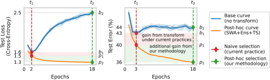
Figure 1: An illustration of the phenomenon of post-hoc reversal on the FMoW dataset: base performance at epoch $t_{2}$ is worse than at epoch $t_{1}$ ($b_{2}>b_{1}$), but post-hoc performance is better ($p_{2}<p_{1}$). The current practice of naive selection considers base metrics to pick models at epoch $t_{1}$. Our proposed methodology of post-hoc selection instead uses post-hoc metrics to pick models at epoch $t_{2}$, resulting in $>2\times$ improvement over naive selection in both test loss and error. SWA+Ens+TS refers to the post-hoc transform obtained by composing SWA, ensemble (Ens) and temperature scaling (TS). Base curves show mean of $8$ runs, models from which constitute the ensembles. Individual runs are shown in lighter colors. See Fig. 5 for more detailed curves on this dataset.

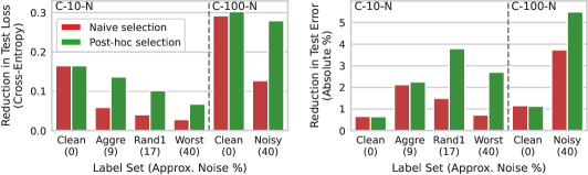
Figure 2: A comparison of naive and post-hoc selection on label sets from CIFAR-10/100-N (abbr. C-10/100-N) for the SWA+TS transform. On noisy label sets, post-hoc selection is often $>2\times$ better.

1 Introduction

Many widely used techniques in deep learning operate on trained models; we refer to these as post-hoc transforms. Examples include temperature scaling (TS) [17], stochastic weight averaging (SWA) [26] and ensembling [36]. These techniques have shown promise for improving predictive performance, robustness, uncertainty estimation, out-of-distribution generalization, and few-shot performance [78, 36, 53, 6, 4]. Typically, the pre-training and post-hoc stages are isolated. The workflow is: (1) pick model architecture, training recipe, hyperparameters, etc. to optimize for individual model performance; (2) train one or more models; (3) pick best-performing checkpoints; (4) apply post-hoc transforms. We refer to this procedure as naive selection.

In this paper, we demonstrate interesting drawbacks of naive selection. In a large-scale empirical study, we uncover post-hoc reversal—a phenomenon whereby post-hoc transforms reverse performance trends between models (Fig. 1). We demonstrate post-hoc reversal with respect to training epochs, model sizes, and other hyperparameters like learning rate schedules. We further establish that post-hoc reversal is a robust phenomenon by experimenting on real-world datasets across domains and modalities, with diverse model classes and training setups.

Post-hoc reversal is most prominent on noisy datasets (Fig. 2). Other phenomena exacerbated by noise include catastrophic overfitting [47], double descent [52], and loss-error mismatch [17]. While these phenomena pose challenges to model development, post-hoc reversal suggests a path to alleviate them. Noise can arise not only from labeling errors, but also from inherent uncertainty in the prediction task, such as in next token prediction [57]. Indeed, severe performance degradation has limited multi-epoch training of large language models (LLMs) [75]. Here too, post-hoc reversal reveals a promising path for sustained performance improvements over longer training.

Based on our findings, we propose post-hoc selection—a simple technique whereby base models are selected based on post-transform performance. The technique is practical as the transforms of interest can be cheaply incorporated into the validation phase of the training loop. Post-hoc selection significantly improves the performance of the transformed models, with $>2\times$ improvements over naive selection in some cases (Fig. 2). In terms of absolute performance, post-hoc selection leads to approx. $4$-point reduction in test error over naive selection on a satellite imaging dataset (Fig. 1). On an LLM instruction tuning dataset, under our procedure a composed transform of SWA, ensemble and TS gives $>1.5\times$ MMLU improvement over a naive application of the same transform on prematurely selected models.

2 Related Work

A slew of empirical works [52, 55, 29, 54, 10, 15] have revealed both challenges and opportunities for improving the understanding and practice of deep learning. Our work expands this list with a novel phenomenon tying together noisy data learning and post-hoc transforms. Orthogonal to our work, a number of training-stage strategies for noisy data have been proposed (see [63] for a survey).

TS belongs to a family of calibration techniques [17, 2, 77] proposed with the goal of producing well-calibrated probabilities. Ensembling is a foundational technique in machine learning, with simple variants routinely used in deep learning [3, 36]. SWA [26] is the culmination of a line of work [16, 23] seeking to cheaply approximate ensembling. Despite their prevalence, a thorough understanding of best practices for wielding these techniques is lacking, especially in the context of noisy data. Our work fills this gap. For a more detailed discussion on related work, see App. A.

3 Preliminaries and Background

We describe our learning setup in § 3.1, with emphasis on noisy data, a key focus of this work. In § 3.2, we introduce the post-hoc transforms we study.

3.1 Learning on Noisy Data

Setup. We consider multi-class classification with $C$ classes, input ${\mathbf{x}}\in{\mathcal{X}}$ and label $y\in{\mathcal{Y}}=\{1,\dots,C\}$. Training, validation and test sets are drawn i.i.d. from the data distribution ${\mathcal{D}}$. A classifier $f\colon\Theta\times{\mathcal{X}}\to{\mathbb{R}}^{C}$ outputs the logit vector ${\mathbf{z}}=f({\mathbf{x}};{\bm{\uptheta}})$, given parameter vector ${\bm{\uptheta}}\in\Theta$. Predicted probability of class $k$ is ${\mathbb{P}}_{f}[y=k\mid{\mathbf{x}}]=\sigma({\mathbf{z}})_{k}$, where $\sigma$ is the softmax function.

Noise. Data ${\mathcal{D}}$ is said to be clean if ${\mathbb{P}}_{\mathcal{D}}[y\mid{\mathbf{x}}]$ is one-hot for all ${\mathbf{x}}$, i.e., ${\mathbb{P}}_{\mathcal{D}}[y\mid{\mathbf{x}}]={\bm{1}}\{y=y^{*}({\mathbf{x}})\}$ for some labeling function $y^{*}\colon{\mathcal{X}}\to{\mathcal{Y}}$. Then, for any example input ${\mathbf{x}}^{(i)}$ in the dataset, the observed label is $y^{(i)}=y^{*}({\mathbf{x}}^{(i)})$. When ${\mathbb{P}}_{\mathcal{D}}[y\mid{\mathbf{x}}]$ is not one-hot, ${\mathcal{D}}$ is said to be noisy and the observed label is only a stochastic sample $y^{(i)}\sim{\mathbb{P}}_{\mathcal{D}}[y\mid{\mathbf{x}}={\mathbf{x}}^{(i)}]$ from the underlying conditional distribution. Noise can arise due to (1) non-determinism in the prediction target (2) insufficient information in the input context, and (3) annotation errors. See App. B.1 for illustrated examples.

Metrics. A metric ${\mathcal{M}}\colon{\mathbb{R}}^{C}\times{\mathcal{Y}}\to{\mathbb{R}}$ compares the predicted logits ${\mathbf{z}}$ with the observed label $y$. ${\mathcal{M}}_{f}({\bm{\uptheta}})={\mathcal{M}}[f({\,\cdot\,};{\bm{\uptheta}})]=\mathop{\mathbb{E}}_{({\mathbf{x}},y)\sim{\mathcal{D}}}[{\mathcal{M}}(f({\mathbf{x}};{\bm{\uptheta}}),y)]$ denotes the metric computed over ${\mathcal{D}}$ given $f$ and ${\bm{\uptheta}}$. We use two metrics (1) classification error, or simply error, with ${\mathcal{M}}^{\text{error}}({\mathbf{z}},y)={\bm{1}}\{\arg\max_{k}{\mathbf{z}}_{k}\not=y\}$ and (2) cross-entropy loss, or simply loss, with ${\mathcal{M}}^{\text{loss}}({\mathbf{z}},y)=-\log\sigma({\mathbf{z}})_{y}$. The exponentiated loss, also called perplexity, is common in language modeling, where it is computed on a per-token basis. A standard result states that loss is minimized if and only if the ground truth conditional probability is recovered [18]. See App. B.1 for additional background.

3.2 Post-Hoc Transforms in Machine Learning

We formally define a post-hoc transform in Def. 1 and give mathematical forms for TS, ensembling and SWA in Eqns. 1, 2 and 3 respectively.

Definition 1 (Post-Hoc Transform)

A post-hoc transform ${\mathcal{T}}$ maps a classifier $f\colon\Theta\times{\mathcal{X}}\to{\mathcal{Y}}$ to another classifier ${\mathcal{T}}\circ f\colon\Theta^{K}\times{\mathcal{X}}\to{\mathcal{Y}}$, for some $K$.

Temperature Scaling (TS). TS [17] involves scaling the logits with a temperature $\tau\in{\mathbb{R}}$ obtained by optimizing the cross-entropy loss over the validation set, with model parameters fixed (Eqn. 1). Temperature scaling preserves error as it does not affect the predicted class.

$$({\mathcal{T}}_{\text{TS}}\circ f)({\mathbf{x}};{\bm{\uptheta}})=\frac{1}{\tau}f({\mathbf{x}};{\bm{\uptheta}}),\text{ with }\tau=\arg\min_{\tau}{\mathcal{M}}_{\text{val}}^{\text{loss}}\left[\frac{1}{\tau}f({\,\cdot\,};{\bm{\uptheta}})\right]$$ (1)

Ensembling. In this method, predictions from an ensemble of classifiers are combined. In deep learning, simply averaging the temperature-scaled logits is effective (Eqn. 2). ${\bm{\uptheta}}_{1},\dots,{\bm{\uptheta}}_{K}$ are obtained from multiple training runs with the same architecture and dataset, with stochasticity from mini-batch sampling and sometimes random initialization.

$$({\mathcal{T}}_{\text{Ens}}\circ f)\left({\mathbf{x}};{\bm{\uptheta}}_{1},\dots,{\bm{\uptheta}}_{K}\right)=\frac{1}{K}\sum_{k=1}^{K}\frac{1}{\tau_{k}}f({\mathbf{x}};{\bm{\uptheta}}_{k}),\text{ with }\tau_{k}=\arg\min_{\tau}{\mathcal{M}}_{\text{val}}^{\text{loss}}\left[\frac{1}{\tau}f({\,\cdot\,};{\bm{\uptheta}}_{k})\right]$$ (2)

Stochastic Weight Averaging (SWA). SWA [26] involves averaging weights ${\bm{\uptheta}}_{1},\dots,{\bm{\uptheta}}_{K}$ from the same training run (Eqn. 3). BatchNorm statistics are recomputed after averaging, if required. Unlike Izmailov et al. [26], we do not skip weights from initial epochs or modify the learning rate schedule.

$$({\mathcal{T}}_{\text{SWA}}\circ f)\left({\mathbf{x}};{\bm{\uptheta}}_{1},\dots,{\bm{\uptheta}}_{K}\right)=f\left({\mathbf{x}};\frac{1}{K}\sum_{i=1}^{K}{\bm{\uptheta}}_{i}\right)$$ (3)

Compositions. TS, ensembling and SWA can be readily composed. In particular, we consider SWA+TS and SWA+Ens+TS, for single- and multi-model settings respectively. We denote them with ${\mathcal{T}}_{\text{S+T}}={\mathcal{T}}_{\text{TS}}\circ{\mathcal{T}}_{\text{SWA}}$ and ${\mathcal{T}}_{\text{S+E+T}}={\mathcal{T}}_{\text{TS}}\circ{\mathcal{T}}_{\text{Ens}}\circ{\mathcal{T}}_{\text{SWA}}$ (explicit forms in App. B.2).

4 Post-Hoc Reversal: Formalization and Empirical Study

To use post-hoc transforms, one must first select models to apply them to. Current practice is to select the best-performing model independent of post-hoc transforms, rationalized by an implicit monotonicity assumption – “better-performing models result in better performance after transformation”. As we shall see, this assumption is often violated in practice. We call such violations post-hoc reversal. In § 4.1, we formalize post-hoc reversal and discuss ways to detect it. In § 4.2, we empirically study various kinds of post-hoc reversal with special practical relevance.

4.1 Definitions

First, we give a general definition of post-hoc reversal (Def. 2). If Def. 2 holds with ${\bm{\upvarphi}}_{k}$’s which are optimal for the base metric ${\mathcal{M}}_{f}$, then naive selection becomes suboptimal as it picks ${\bm{\upvarphi}}_{k}$’s, but ${\bm{\uptheta}}_{k}$’s are better under the post-hoc metric ${\mathcal{M}}_{{\mathcal{T}}\circ f}$. Since the entire space of parameter tuples $\Theta^{K}$ can be large, we study post-hoc reversal restricted to indexed parameters (Def. 3). Indices can be, for example, training epochs (§ 4.2.1), model sizes (§ 4.2.2) or hyperparameter configurations (§ 4.2.3).

Definition 2 (Post-hoc reversal)

Let a post-hoc transform ${\mathcal{T}}$ map a classifier $f\colon\Theta\times{\mathcal{X}}\to{\mathcal{Y}}$ to ${\mathcal{T}}\circ f\colon\Theta^{K}\times{\mathcal{X}}\to{\mathcal{Y}}$. ${\mathcal{T}}$ applied to $f$ exhibits post-hoc reversal for a metric ${\mathcal{M}}$ if there exist $({\bm{\uptheta}}_{1},\dots,{\bm{\uptheta}}_{K}),({\bm{\upvarphi}}_{1},\dots,{\bm{\upvarphi}}_{K})\in\Theta^{K}$ such that ${\mathcal{M}}_{f}({\bm{\uptheta}}_{k})\geq{\mathcal{M}}_{f}({\bm{\upvarphi}}_{k})$ for all $k=1,\dots,K$ but ${\mathcal{M}}_{{\mathcal{T}}\circ f}({\bm{\uptheta}}_{1},\dots,{\bm{\uptheta}}_{K})<{\mathcal{M}}_{{\mathcal{T}}\circ f}({\bm{\upvarphi}}_{1},\dots,{\bm{\upvarphi}}_{K})$.

Definition 3 (Index-wise post-hoc reversal)

Let ${\mathcal{I}}$ be a set of indices and ${\mathcal{P}}\colon{\mathcal{I}}\to\Theta^{K}$ map indices to parameter tuples. When Def. 2 holds with $({\bm{\uptheta}}_{1},\dots,{\bm{\uptheta}}_{K})={\mathcal{P}}(s),({\bm{\upvarphi}}_{1},\dots,{\bm{\upvarphi}}_{K})={\mathcal{P}}(t)$ for some $s,t\in{\mathcal{I}}$, we call it index-wise post-hoc reversal.

Diagnosis. To enable a visual diagnosis of post-hoc reversal, we define base and post-hoc curves (Def. 4) and a relaxed notion of post-hoc reversal for them (Def. 5). Post-hoc reversal is characterized by non-monotonicity between the base and post-hoc curves, i.e., there exist regions where one improves while the other worsens. This happens, for instance, when one curve exhibits double descent but the other doesn’t. Different optimal indices for the two curves is another indicator of post-hoc reversal.

Definition 4 (Base and post-hoc curves)

The base and post-hoc curves ${\mathcal{M}}^{\text{base}},{\mathcal{M}}^{\text{post}}\colon{\mathcal{I}}\to{\mathbb{R}}$ are given by ${\mathcal{M}}^{\text{base}}(t)=\frac{1}{K}\sum_{k=1}^{K}{\mathcal{M}}_{f}({\bm{\uptheta}}_{k})$ and ${\mathcal{M}}^{\text{post}}(t)={\mathcal{M}}_{{\mathcal{T}}\circ f}({\bm{\uptheta}}_{1},\dots,{\bm{\uptheta}}_{K})$, where $({\bm{\uptheta}}_{1},\dots,{\bm{\uptheta}}_{K})={\mathcal{P}}(t)$.

Definition 5 (Post-hoc reversal for curves)

Base and post-hoc curves ${\mathcal{M}}^{\text{base}},{\mathcal{M}}^{\text{post}}\colon{\mathcal{I}}\to{\mathbb{R}}$ exhibit post-hoc reversal when there exist $s,t\in{\mathcal{I}}$ such that ${\mathcal{M}}^{\text{base}}(s)\geq{\mathcal{M}}^{\text{base}}(t)$ but ${\mathcal{M}}^{\text{post}}(s)<{\mathcal{M}}^{\text{post}}(t)$.

4.2 Experiments

4.2.1 Epoch-Wise Post-Hoc Reversal

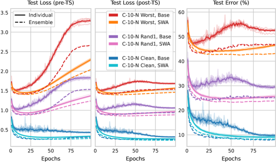
Figure 3: Loss and error for CIFAR-10-N Clean (approx. $0\%$ noise), Rand1 (approx. $17\%$ noise) and Worst (approx. $40\%$ noise). Except for ensemble curves, mean of $8$ runs is shown; individual runs are in lighter shades. Ensembles comprise models from these $8$ runs. For example, observe post-hoc reversal for C-10-N Worst: (1) error plot: from epoch $5$ to $50$, solid red (base) curve worsens but solid orange (SWA) curve improves; (2) error plot: solid red (base) curve has a double descent but dashed red (ensemble) curve does not; (3) loss plots: solid red (base) curve has a double descent pre-TS but not post-TS; (4) error plot: best error is at approx. epoch $5$ for solid red (base) curve but at approx. epoch $60$ for dashed orange (SWA ensemble) curve.

When the indices in Def. 3 are training epochs, we call it epoch-wise post-hoc reversal. We use ${\bm{\uptheta}}_{t}$ to denote the model at the end of epoch $t$. For ensembles, a superscript $j$ denotes the $j$-th training run (out of $N$ runs). $t\in{\mathcal{I}}$ maps to parameters ${\mathcal{P}}(t)\in\Theta^{K}$ ($K=1$ for TS; $N$ for ensemble; and $t$ for SWA) as follows: ${\mathcal{P}}_{\text{TS}}(t)=({\bm{\uptheta}}_{t})$; ${\mathcal{P}}_{\text{Ens}}(t)=({\bm{\uptheta}}_{t}^{1},\dots,{\bm{\uptheta}}_{t}^{N})$.; ${\mathcal{P}}_{\text{SWA}}(t)=({\bm{\uptheta}}_{1},\dots,{\bm{\uptheta}}_{t})$.

Experimental setup. We focus on the CIFAR-N dataset [68]. CIFAR-10-N uses the same images as CIFAR-10 but provides multiple human-annotated label sets, allowing the study of realistic noise patterns of varying levels in a controlled manner. Clean is the original label set; Rand1,2,3 are 3 sets of human labels; Aggre combines Rand1,2,3 by majority vote; and Worst combines them by picking an incorrect label, if possible. Similarly CIFAR-100-N has two label sets, Clean and Noisy, with the latter being human-labeled. We train ResNet18 [19] models for 100 epochs with a cosine annealed learning rate. Additional details on datasets and training setup are in App. C. Fig. 3 shows test curves on CIFAR-10-N Clean, Rand1 and Worst. Other label sets and CIFAR-100-N are in App. E. For clarity, we omit the SWA base curve ${\mathcal{M}}_{\text{SWA}}^{\text{base}}(t)=({\mathcal{M}}_{f}({\bm{\uptheta}}_{1})+\dots+{\mathcal{M}}_{f}({\bm{\uptheta}}_{t}))/t$ in the plots, and simply re-use the curve ${\mathcal{M}}^{\text{base}}(t)={\mathcal{M}}_{f}({\bm{\uptheta}}_{t})$ to compare with the post-hoc SWA curve. While deviating from Def. 4, this better reflects the current practice of early stopping on the latest epoch’s base metric.

Observations. First, we focus on the base curves: (1) Overfitting: As noise increases, test curves go from a single descent to a double descent to a U-shaped curve with increased overfitting. (2) Double descent: Noise amplifies double descent, and the second descent worsens with increasing noise (as compared to the first). (3) Loss-error mismatch: Loss overfits more drastically than error, leading to a mismatch with higher noise. Optimal models for loss and error can be different.

Next, we consider the general impact of post-hoc transforms: (4) Performance improvements: TS, SWA and ensemble always improve performace, both individually and in composition with larger gaps for noisy label sets. (5) Post-hoc reversal: Post-hoc reversal manifests as non-monotonicity between the base and post-hoc curves, especially for noisy label sets. (6) SWA vs Ensemble: SWA can recover much of the ensemble gain, but the optimal epoch often differs a lot from the base curve. (7) Smoother curves: Base curves fluctuate wildly, but SWA and ensemble curves are smooth, making them more reliable for early stopping.

Finally, we discuss some benefits from post-hoc reversal: (8) Overfitting: All transforms reduce overfitting, often reverting performance degradation. (9) Double descent: SWA, ensemble and compositions flatten the double descent peak. TS, on the other hand, leads to a double descent for some cases where there was none before. (10) Loss-error mismatch: TS aligns the loss and error curves, enabling simultaneously good loss and error.

4.2.2 Model-Wise Post-Hoc Reversal

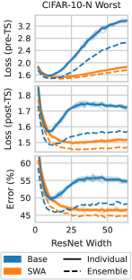
Figure 4: C-10-N Worst test curves against model size. Best width for solid blue curves is approx. $10$ but for dashed orange curves, it is approx. $50$ for error and approx. $25$ for post-TS loss.

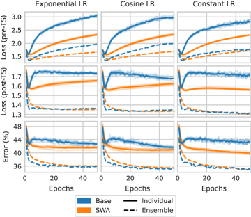
Figure 5: FMoW test curves for $3$ LR schedules. Note that the pre-TS loss is significantly higher than the post-TS loss. For example, observe post-hoc reversal w.r.t. cosine and constant LRs at epoch $50$ between: (1) solid blue (base) and dashed blue (ensemble) error curves; (2) solid blue (base) and solid orange (SWA) post-TS loss curves; (3) solid blue (base) curves for pre-TS and post-TS loss.

Here, indices represent model sizes. Models of all sizes are trained for $T$ epochs, large enough for convergence. Following [52], we avoid early stopping. Notation-wise, we add a subscript to ${\bm{\uptheta}}$ to indicate the model size $s$. Parameters are indexed as follows: ${\mathcal{P}}_{\text{TS}}(s)=({\bm{\uptheta}}_{T,s})$; ${\mathcal{P}}_{\text{Ens}}(s)=({\bm{\uptheta}}_{T,s}^{1},\dots,{\bm{\uptheta}}_{T,s}^{N})$; ${\mathcal{P}}_{\text{SWA}}(s)=({\bm{\uptheta}}_{1,s},\dots,{\bm{\uptheta}}_{T,s})$.

Experimental setup. We parameterize a family of ResNet18s by scaling the number of filters in the convolutional layers. Specifically, we use $[k,2k,4k,8k]$ filters for width $k$. The standard ResNet18 corresponds to $k=64$. Otherwise the training setup is same as before. Fig. 5 shows the curves. Concretely, the index set ${\mathcal{I}}=\{2,4,\dots,64\}$ is the set of ResNet widths $k$ described above.

Observations. Post-hoc transforms improve performance (up to $\approx 10$ points for error) and mitigate double descent. Further, we see yet another way in which higher-capacity models are better: they give better results under post-hoc transforms even when lower-capacity base models perform better.

4.2.3 Hyperparameter-Wise Post-Hoc Reversal

In general, the index set ${\mathcal{I}}$ can contain any hyperparameter configurations. Here, we consider two hyperparamters: learning rate schedule and training epochs. To avoid repeating CIFAR-N epoch-wise curves, we experiment on a fresh dataset, FMoW.

Experimental setup. We experiment on learning rates (LRs) and training epochs, with index set ${\mathcal{I}}=\{\texttt{const},\texttt{exp},\texttt{cos}\}\times\{1,\dots,T\}$. Here, const, exp and cos refer to constant, exponentially decaying and cosine annealed LRs respectively, and $T$ is the total number of epochs. We train DenseNet121 [24] models on the FMoW dataset [9] which constitutes a $62$-way classification of land use from satellite images. For more details, see App. C. Fig. 5 shows the curves.

LR-wise observations. We see some interesting instances of post-hoc reversal: (1) constant LR has the worst base performance but the best post-hoc performance; (2) under SWA and TS (composed), the curves continue to improve at the later epochs for constant LR, but not for the decaying LRs.

Epoch-wise observations. Epoch-wise post-hoc reversal occurs for all LR schedules. SWA and ensembling convert the double descent into a strong single descent, with approx. $10$-point improvement in error for the latter. For constant LR, this also changes the optimal epoch. SWA only recovers about half of the ensemble gain, and perhaps surprisingly, ensembling SWA models is not better than ensembling alone. Pre-TS loss curves show a strong mismatch with the error curves, but TS enables simultaneously good loss and error with the last epoch models. Overall, these observations reinforce the trends gleaned from the CIFAR-N experiments.

5 Post-Hoc Selection: Leveraging Post-Hoc Reversal in Practice

C-10-N Clean&0.435$\bm{0.269}$0.2700.234$\bm{0.233}$9.75$\bm{9.09}$9.108.30$\bm{8.24}$
C-10-N Aggre0.7220.663$\bm{0.585}$0.608$\bm{0.543}$19.2017.08$\bm{16.95}$15.88$\bm{15.74}$
C-10-N Rand11.0090.968$\bm{0.907}$0.916$\bm{0.859}$28.6327.13$\bm{24.84}$24.80$\bm{23.50}$
C-10-N Worst1.5111.483$\bm{1.443}$1.437$\bm{1.399}$46.8446.12$\bm{44.14}$44.30$\bm{42.88}$
C-100-N Clean1.5081.215$\bm{1.205}$1.065$\bm{1.063}$33.83$\bm{32.67}$32.69$\bm{29.90}$29.94
C-100-N Noisy2.4162.289$\bm{2.136}$2.129$\bm{1.994}$58.6854.94$\bm{53.18}$51.34$\bm{50.26}$
FMoW1.5831.627$\bm{1.554}$1.494$\bm{1.305}$43.2042.69$\bm{39.92}$37.95$\bm{34.93}$
Metric $\rightarrow$ Test Loss Test Error (%) Transform $\rightarrow$ None SWA+TS SWA+Ens+TS None SWA+TS SWA+Ens+TS Dataset $\downarrow$ Naive Ours Naive Ours Naive Ours Naive Ours

Table 1: Naive vs post-hoc (ours) selection for SWA+TS and SWA+Ens+TS transforms. Better values are in bold. Except some clean cases, post-hoc selection is always better, often more than doubling the improvement over no transform as compared to naive selection. See Tab. E and E in App. E for standard deviations.

Our findings from §4 motivate the principle of post-hoc selection, where model development decisions take post-hoc transforms into account. For concreteness, we discuss the choice of checkpoints from training runs under the SWA+TS and SWA+Ens+TS transforms. Checkpoint selection reduces to the selection of the final epoch $\widehat{T}$, as SWA uses all checkpoints up to that epoch. ${\mathcal{M}}_{\text{val}}$ denotes a metric of choice computed on the validation set.

SWA+TS. Naive selection picks epoch $\widehat{T}=\arg\min_{T}{\mathcal{M}}_{f}^{\text{val}}({\bm{\uptheta}}_{T})$. In contrast, post-hoc selection picks $\widehat{T}=\arg\min_{T}{\mathcal{M}}_{{\mathcal{T}}_{\text{S+T}}\circ f}^{\text{val}}(({\bm{\uptheta}}_{t})_{t=1}^{T})$.

SWA+Ens+TS. Here we have $N$ different training runs to pick epochs for. Naive selection picks $\widehat{T}_{j}=\arg\min_{T}{\mathcal{M}}_{f}^{\text{val}}({\bm{\uptheta}}_{T}^{j})$ for each run independently. In contrast, post-hoc selection would ideally pick $\widehat{T}_{1},\ldots,\widehat{T}_{N}=\arg\min_{T_{1},\dots,T_{N}}{\mathcal{M}}_{{\mathcal{T}}_{\text{S+E+T}}\circ f}^{\text{val}}(({\bm{\uptheta}}_{t}^{1})_{t=1}^{T_{1}},\dots,({\bm{\uptheta}}_{t}^{N})_{t=1}^{T_{N}})$ which jointly minimizes the ensemble performance. This being computationally expensive, we instead minimize under the constraint $\widehat{T}_{1}=\dots=\widehat{T}_{N}$

Results. Tab. 5 compares naive and post-hoc selection strategies for CIFAR-N and FMoW. Except for some clean label sets, post-hoc selection is always better than naive selection, often with $>2\times$ improvement from post-hoc selection as compared to naive selection.

Early stopping. We advocate monitoring post-hoc metrics for early stopping. Only a running average needs to be updated for SWA, and TS involves a quick single-parameter optimization. Further, while the base curves can fluctuate wildly between consecutive runs, SWA+TS curves are considerably smoother (see Figs. 3, 9 and 7), making them more reliable for automated early stopping. One can similarly monitor metrics for SWA+Ens+TS under parallel training runs.

6 Experiments Across Domains and Modalities

In § 4 and § 5, we introduced post-hoc reversal and selection with experiments on the CIFAR-N and FMoW datasets. In this section, we supplement our experimental analysis with additional experiments across diverse domains and modalities to demonstrate the generality of our findings.

6.1 LLM Instruction Tuning

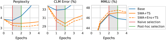
Figure 6: Perplexity and causal language modeling (CLM) error on the Guanaco test set, and MMLU accuracy (higher is better) for instruction tuning LLaMA-2-7B. Shading indicates post-hoc reversal. Base and SWA+TS curves are mean of $8$ runs. Individual runs are not shown as they would largely overlap with the mean curve (max range among runs: 0.01 perplexity, 0.07 error, 0.13 MMLU). SWA+Ens+TS curves ensemble models from these $8$ runs.

Language models are pre-trained or fine-tuned with a self-supervised objective of predicting the next token in a text corpus. There might be many acceptable tokens following a given prefix, albeit with different probabilities. Thus next token prediction is noisy and one might reasonably expect to see post-hoc reversal. In this section, we test this hypothesis for the task of fine-tuning LLMs to follow instructions (instruction tuning [66]). Instruction tuning datasets are naturally small and amenable to multi-epoch training where catastrophic overfitting becomes an important concern. Recent works [50, 75] have argued for data repetitions for LLM pre-training as well, and we expect post-hoc reversal to occur there too, with important consequences. However, such experiments are beyond the scope of this paper.

Experimental setup. We fine-tune LLaMA-2-7B [64] on the Guanaco dataset [12] of chat completions. We evaluate perplexity and causal language modeling (CLM) error on the test set, and also the MMLU accuracy [22] to better contextualize model improvements. Fig. 6 shows the curves. Tab. 7 in App. E gives exact numbers.

Observations. We observe post-hoc reversal between epochs 1 and 2 for perplexity and error, and between epochs 2 and 3 for MMLU. Both SWA+TS and SWA+Ens+TS transforms show significant improvements, much of which is only realized under post-hoc selection.

6.2 Other Text, Tabular and Graph Datasets

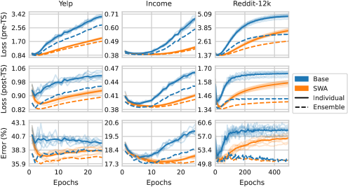
Figure 7: Test curves for 3 real-world noisy datasets. Note that the pre-TS loss is significantly higher than the post-TS loss. Examples of post-hoc reversal between the base curves given by the solid blue lines and the post-hoc curves given by the dashed orange lines (SWA ensemble): (1) optimal epoch is different for base and post-hoc curves for error and post-TS loss on all datasets; (2) for error on Yelp, base curve shows double descent but post-hoc curve does not; (3) for error on Income, base curve overfits catastrophically at approx. epoch $5$ but post-hoc curve continues improving till approx. epoch $20$; (4) for error on Reddit-12k, base curve does not show double descent but post-hoc curve does.

In this section, we further expand our experimental coverage to text, tabular and graph classification datasets from real-world applications.

Experimental setup. We consider the following tasks: (1) sentiment classification on the Yelp reviews dataset [5] (text) with a pre-trained transformer BERT [13], (2) prediction tasks on census data from Folktables [14] (tabular) with MLPs and (3) community detection on the Reddit and Collab datasets [76] (graph) with graph neural networks (GNNs). Folktables has 5 prediction tasks: Income, PublicCoverage, Mobility, Employment and TravelTime. Reddit has 2 versions: Reddit-5k and Reddit-12k. For more details, see App. C. Figure 7 shows curves for Yelp, Income and Reddit-12k. Tab. D in App. D compares naive and post-hoc selection on all datasets.

Observations. Post-hoc reversal is a recurring feature across datasets, transforms and metrics. The 3 datasets show different patterns between the base and post-hoc curves, showing that post-hoc reversal can take a variety of forms.

7 Conclusion

We empirically studied temperature scaling (TS), ensembling, stochastic weight averaging (SWA) and their compositions, and found that these transforms can reverse model peformance trends (post-hoc reversal). Based on our findings, we presented the simple technique of post-hoc selection, and showed that it outperforms naive selection. We validated our findings and proposals over a wide variety of experimental settings.

Our work has broad implications for the field of deep learning. It shows that current practices surrounding the use of post-hoc transforms leave much room for improvement. This is especially true for noisy data, which is pervasive in real-world applications. More broadly, post-hoc reversal challenges our understanding of neural network training dynamics and calls for rethinking deep learning workflows. For example, an interesting question for future research is how post-hoc reversal impacts scaling laws, which are crucially relied on for compute allocation in large-scale training runs. Other future directions include better strategies for checkpoint selection, understanding the theoretical underpinnings of post-hoc reversal, and characterizing other instances of it.

Summary of practical recommendations. We advocate for the use of TS, ensembling and SWA across deep learning applications. Further, such transforms should be tightly integrated into the model development pipeline, following the methodology outlined in the paper. In particular: (1) apply SWA+TS and SWA+Ens+TS transforms for better results in the single- and multi-model settings respectively; (2) track temperature-scaled loss to overcome loss-error mismatch; (3) monitor post-hoc metrics to avoid premature early stopping; (4) make hyperparameter decisions informed by post-transform performance; (5) use post-hoc selection to pick model checkpoints.

Appendix A Expanded Related Work

Phenomena. Empirical works like double descent [52], grokking [55], scaling laws [29], neural-collapse [54], edge-of-stability [10], lottery-ticket-hypothesis [15] have revealed both challenges and oppotunities for improving the understanding and practices of deep neural network training. Post-hoc reversal expands this list as a novel phenomenon regarding learning dynamics under the lens of post-hoc transforms. It is most intimately connected with double descent, offering a way to mitigate it. Some works [70, 61, 51, 21, 7, 56] show other mitigations, such as regularization and data augmentation.

Temperature Scaling (TS). TS belongs to a family of post-hoc calibration techniques [17, 2, 77], with the unique property of preserving classification error. Recently, calibration has been applied to large vision and language models [11, 78, 65]. While loss-error mismatch has been reported before [17, 11], to the best of our knowledge, we are the first to report post-hoc reversal with TS.

Ensembling. Ensembling is a foundational technique in machine learning, encompassing bagging, boosting, etc. In deep learning, a uniform ensemble is most popular [3, 36], although recent work on ensembling LLMs has explored more efficient routing-based ensembles [43, 46, 27, 45]. Various works have explored strategies to form optimal ensembles [44, 33, 48, 71], generally based on model diversity [35], but recently Abe et al. [1] have warned against this. In contrast, our recommendation for forming ensembles relies directly on the validation performance of the ensemble, introducing no proxies, and still being computationally cheap.

Stochastic Weight Averaging (SWA). SWA [26] is the culmination of a line of work [16, 23] which seek to cheaply approximate ensembling. It has inspired numerous works which average weights in some form [38, 25, 71, 58, 6, 4] often in combination with ensembling. Recently, weight averaging has shown up in the LLM space [60, 59]. While these works generally apply SWA with a fixed training time determined independently, we present SWA in the role of early stopping and model selection. In practice, SWA has often been found to be unreliable, and is often skipped from training recipes even when considered [32, 69]. Our work sheds some light on this, offering a rather counter-intuitive choice of models to include in the weight average for best results.

Label noise. Many training strategies have been introduced to deal with noisy data (see [63] for a survey). However, the efficacy of simple post-hoc transforms has been left unexplored. Further, most of these works are motivated by labeling errors, which leaves some of the core practical considerations for dealing with general noisy data unaddressed. For instance, access to a clean validation set is assumed and test loss is overlooked as an important metric [40, 41]. We also entirely avoid experiments on synthetic noise, informed by recent work which questions the transferability of findings to realistic noise patterns [28, 67]. Some recent datasets [28, 67, 73, 37, 62] make it possible to study realistic noise along with known noise estimates.

Multi-epoch training of LLMs. Multi-epoch training of LLMs runs into severe catastrophic overfitting. Xue et al. [75] examine the contributing factors and explore possible solutions. They find that regularization is not helpful, except for dropout. Muennighoff et al. [50] study scaling laws considering data repetitions. Complementarily, we put forward post-hoc transforms as an effective solution with our post-hoc selection methodology. This is especially important for fine-tuning LLMs, e.g. in instruction tuning [66], where [79] and [8] advocate for fine-tuning with a smaller amount of higher quality samples for more epochs.

Appendix B Expanded Preliminaries and Background

B.1 Learning on Noisy Data

Figure 8: Data can be noisy due to non-determinism in the prediction target (aleatoric uncertainty). Figure shows a message tree from the OpenAssistant Converstations (OASST1) Dataset. A chatbot can continue a conversation satisfactorily in many different ways, making next token prediction noisy.

(a) Gas Station

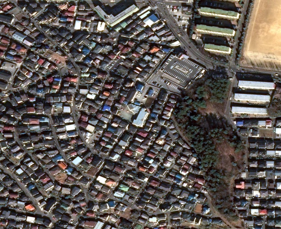
(b) Educational Institution

Figure 9: Data can be noisy due to insufficient information in the input context (epistemic uncertainty). Figures 9(a) and 9(b) show satellite images from the FMoW dataset. The labels are correct, as corroborated by external map data. However, they cannot be determined with full certainty from the images alone.

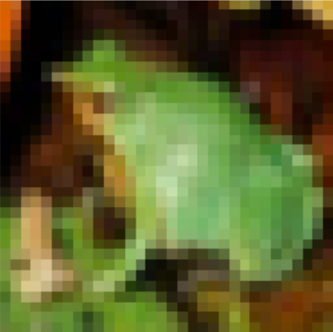
(a) L: Cat
C: Frog

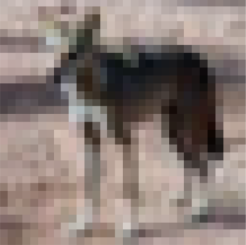
(b) L: Horse
C: Deer

(c) L: Airplane
C: Ship

(d) L: Bee
A: Sunflower

(e) L: Dolphin
A: Woman

(f) L: Mountain
A: Cloud

Figure 10: Data can be noisy due to annotation errors. Figures 10(a), 10(b) and 10(c) are mislabeled images from CIFAR-10. 10(d), 10(e) and 10(f) are ambiguous images from CIFAR-100 with multiple correct labels among the given classes. (L = label in dataset, C = correct label, A = alternative label)

Figures 9, 9 and 10 illustrate various sources of noise: aleatoric unertainty, epistemic uncertainty and annotation errors. Below we provide some background on Bayes-optimal classifier and use it to introduce the clean error metric and Bayes loss/error as measures of noise level.

Bayes-optimal classifier. $f_{\mathcal{D}}$, given by $f_{\mathcal{D}}({\mathbf{x}})_{k}=\log{\mathcal{P}}_{\mathcal{D}}[y=k\mid{\mathbf{x}}]$ minimizes both ${\mathcal{M}}_{\mathcal{D}}^{\text{error}}$ and ${\mathcal{M}}_{\mathcal{D}}^{\text{loss}}$, and is called the Bayes-optimal classifier for ${\mathcal{D}}$. The Bayes error ${\mathcal{M}}_{\mathcal{D}}^{\text{error}}[f_{\mathcal{D}}]$ and Bayes loss ${\mathcal{M}}_{\mathcal{D}}^{\text{loss}}[f_{\mathcal{D}}]$ are measures of the noise level. $y^{*}({\mathbf{x}})=\arg\max_{k}f_{\mathcal{D}}({\mathbf{x}})_{k}$ is sometimes called the clean label. Using $y^{*}$, one may define the clean data distribution ${\widetilde{\mathcal{D}}}$ with ${\mathcal{P}}_{\widetilde{\mathcal{D}}}[{\mathbf{x}}]={\mathcal{P}}_{\mathcal{D}}[{\mathbf{x}}]$ and ${\mathcal{P}}_{\widetilde{\mathcal{D}}}[y\mid{\mathbf{x}}]={\bm{1}}\{y=y^{*}({\mathbf{x}})\}$. The clean error ${\mathcal{M}}_{\widetilde{\mathcal{D}}}^{\text{error}}$ is a common metric in the label noise literature but not a focus of our work as $y^{*}$ is typically inaccessible in more general noisy settings.

B.2 Post-Hoc Transforms in Machine Learning

The explicit forms of the composed transforms SWA+TS and SWA+Ens+TS (denoted as ${\mathcal{T}}_{\text{S+T}}$ and ${\mathcal{T}}_{\text{S+E+T}}$) are given by Equations 4 and 5 respectively. For ${\mathcal{T}}_{\text{S+E+T}}$, parameters ${\bm{\uptheta}}_{1}^{l},\dots,{\bm{\uptheta}}_{K_{l}}^{l}$ are weight-averaged and the $L$ resulting models are ensembled, followed by temperature scaling. $\tau_{l}$ is the temperature for weight-averaged models, and $\tau_{\text{Ens}}$ is the temperature for the ensemble. As before, they are obtained by optimizing the cross-entropy loss over the validation set, with model parameters fixed.

$$({\mathcal{T}}_{\text{S+T}}\circ f)\left({\mathbf{x}};{\bm{\uptheta}}_{1},\dots,{\bm{\uptheta}}_{K}\right)=\frac{1}{\tau}f\left({\mathbf{x}};\frac{1}{K}\sum\limits_{i=1}^{K}{\bm{\uptheta}}_{i}\right),\text{ with }\tau=\arg\min_{\tau}{\mathcal{M}}_{\text{val}}^{\text{loss}}\left[\frac{1}{\tau}f\left({\,\cdot\,};\frac{1}{K}\sum\limits_{i=1}^{K}{\bm{\uptheta}}_{i}\right)\right]$$ (4)

$$({\mathcal{T}}_{\text{S+E+T}}\circ f)\left({\mathbf{x}};{\bm{\uptheta}}_{1}^{1},\dots,{\bm{\uptheta}}_{K_{1}}^{1},\dots,{\bm{\uptheta}}_{1}^{L},\dots,{\bm{\uptheta}}_{K_{L}}^{L}\right)=\frac{1}{\tau_{\text{Ens}}}\frac{1}{L}\sum_{l=1}^{L}\frac{1}{\tau_{l}}f\left({\mathbf{x}};\frac{1}{K_{l}}\sum\limits_{k=1}^{K_{l}}{\bm{\uptheta}}_{k}^{l}\right)$$ (5)

Appendix C Dataset and Training Details

Vision CIFAR-10 $40000$ $5000$ $5000$ $10$ $3\times 32\times 32$ C $\times$ W $\times$ H
CIFAR-100-N Coarse $40000$ $5000$ $5000$ $20$ $3\times 32\times 32$
CIFAR-100-N Fine $40000$ $5000$ $5000$ $100$ $3\times 32\times 32$
FMoW $76863$ $11483$ $11327$ $62$ $3\times 224\times 224$
Text Guanaco $8850$ $500$ $500$ $32000$ $\lesssim 4000$ characters
Yelp $25000$ $5000$ $5000$ $5$ $\lesssim 2000$
Tabular Income $156533$ $19566$ $19566$ $2$ $816$ features
Public Coverage $110844$ $13855$ $13855$ $2$ $88$
Mobility $64265$ $8032$ $8032$ $2$ $101$
Employment $303055$ $37881$ $37881$ $2$ $98$
Travel Time $138008$ $17250$ $17250$ $2$ $615$
Graph Collab $4000$ $500$ $500$ $3$ $74.49$, $2457.78$ nodes, edges (avg.)
Reddit-5k $4001$ $499$ $499$ $5$ $508.52$, $594.87$
Reddit-12k $9545$ $1192$ $1192$ $11$ $391.41$, $456.89$
Modality Dataset Train Size Val Size Test Size Classes Input Size Units

Table 2: Dataset Details.

C-10/100-N ResNet18-D [20] Yes SGD 0.1 5e-4 Cosine 100 500
FMoW DenseNet121 [24] Yes Adam 1e-4 0 Constant 50 64
Guanaco LLaMA-2-7B [64] Yes Adam 2e-4 0 Constant 6 16
Yelp BERT [13] Yes AdamW 5e-5 1e-2 Linear 25 16
Folktables MLP No Adam 0.01 0 Exponential 50 256
Collab GIN [74] No Adam 0.01 0 Exponential 500 128
Reddit GCN [30] No Adam 0.01 0 Exponential 500 128
Dataset Model Pre- train Optimizer LR Weight Decay LR Schedule Epochs Batch Size

Table 3: Training Details.

Table 4: Noise levels for CIFAR-N (%), reproduced from [68].

CIFAR-10-N						CIFAR-100-N Coarse		CIFAR-100-N Fine
Clean	Aggre	Rand1	Rand2	Rand3	Worst	Clean	Noisy	Clean	Noisy
0.00	9.03	17.23	18.12	17.64	40.21	0.00	25.60	0.00	40.20

Tables C and 3 summarize the datasets and training details for our experiments. They are described in detail below.

CIFAR-N [68]. CIFAR-10-N uses the same images as CIFAR-10 but provides multiple human-annotated label sets. Clean is the original label set; Rand1,2,3 are 3 sets of human labels; Aggre combines Rand1,2,3 by majority vote; and Worst combines them by picking an incorrect label, if possible. CIFAR-100 has 2 variants, a fine-grained one with 100 classes and a coarse-grained one with 20 classes, obtained by grouping the fine-grained classes. Correspondingly, there are CIFAR-100-N Coarse and CIFAR-100-N Fine datasets. They have two label sets each: Clean and Noisy, with the latter being human-labeled. In the main paper, CIFAR-100-N refers to the fine-grained version.

By cross-referencing with the original labels, it is possible to estimate the noise levels. These are shown in Table 4.

CIFAR-N allows access to clean labels. In the literature, the validation and test sets for CIFAR-N typically use the clean labels [72, 39, 42]. However, access to clean labels is a luxury only available for label noise settings. Even there, obtaining clean labels is expensive, as it requires careful expert annotation. For other sources of noise it might not even be feasible to obtain clean labels. Hence, we restrict ourselves to using noisy (i.i.d. to train) validation and test sets. Since CIFAR-N only provides human labels for the original 50k CIFAR-10/100 train images, we split these into 40k/5k/5k images for train/val/test sets.

FMoW [9, 31]. This is the version of the original FMoW dataset [9] as used in the WILDS benchmark [31]. The input is an RGB satellite image (rescaled to 224 x 224 pixels) and the label is one of 62 building or land use categories. The labels were obtained by a combination of human annotation and cross-referenced geographical information. The original dataset provides additional metadata about location, time, sun angles, physical sizes, etc. which is ignored in the WILDS dataset (and hence in ours). While the labels have low noise compared to the ground-truth, this dataset is noisy because of insufficient information. It is hard to disambiguate the building or land use category with full certainty by looking at the satellite image alone. See Figure 9. Models and training setup are as used in [9, 31], except for the LR schedule, where we experiment with multiple alternatives.

Guanaco [12]. This is a subset of the OASST1 dataset [34] containing only the highest-rated paths in the conversation tree. We follow the fine-tuning setup from [12], except that we use vanilla fine-tuning without any quantization or low-rank adapters.

Yelp [5]. This is a subset of the Yelp Dataset Challenge 2015 dataset with 25k reviews in the train set and 5k reviews each in the validation and test sets. The input is a review text and the label is one of 5 classes (1 to 5 stars). Assigning a rating to a review is intrinsically non-deterministic as different reviewers might have different thresholds for the star ratings. This introduces noise in the data.

Folktables [14]. Folktables consists of 5 classification tasks based on the US Census: Income, Employment, Health, TravelTime and PublicCoverage. The data is tabular. The available feature columns do not contain sufficient information to predict the targets with full certainty, even if the Census recorded the ground-truth labels with high accuracy. This results in noise. See Figure LABEL:fig:noise_bench/fmow_adult.

Collab and Reddit [76, 49]. These datasets are from TUDataset [49], and were originally introduced by Yanardag and Vishwanathan [76]. Collab is a scientific collaboration dataset. The input is an ego-network of a researcher and the label is the field of the researcher (one of High Energy Physics, Condensed Matter Physics and Astro Physics). The Reddit-5k and Reddit-12k datasets (originally called REDDIT-MULTI-5K and REDDIT-MULTI-12K) are balanced datasets where the input is a graph which corresponds to an online discussion thread from the social network site Reddit. Nodes correspond to users and there is an edge if one user responded to another’s comment. The task is to predict which subreddit a discussion graph belongs to. Reddit-5k is smaller with 5k examples and 5 classes. Reddit-12k is bigger with 12k examples and 11 classes.

Appendix D Post-Hoc Selection Results for Remaining Datasets

Yelp0.9080.890$\bm{0.854}$0.841$\bm{0.824}$39.4138.02$\bm{37.33}$36.18$\bm{36.14}$
Income0.3930.390$\bm{0.387}$0.388$\bm{0.385}$17.8417.69$\bm{17.54}$17.62$\bm{17.40}$
PublicCoverage0.5440.540$\bm{0.539}$0.538$\bm{0.538}$27.5227.31$\bm{27.25}$27.25$\bm{27.02}$
Mobility0.4740.472$\bm{0.471}$0.471$\bm{0.468}$21.43$\bm{21.38}$21.42$\bm{21.17}$21.24
Employment0.3800.379$\bm{0.378}$0.378$\bm{0.377}$17.94$\bm{17.77}$17.80$\bm{17.72}$17.83
TravelTime0.5970.597$\bm{0.593}$0.596$\bm{0.591}$35.7735.46$\bm{35.35}$35.44$\bm{35.23}$
Collab0.4920.475$\bm{0.460}$0.439$\bm{0.404}$20.6521.58$\bm{20.27}$20.40$\bm{18.80}$
Reddit-5k1.1541.112$\bm{1.100}$1.101$\bm{1.085}$47.4248.35$\bm{47.04}$47.09$\bm{45.49}$
Reddit-12k1.4051.381$\bm{1.366}$1.367$\bm{1.346}$51.78$\bm{51.08}$51.11$\bm{50.34}$51.26
Metric $\rightarrow$ Test Loss Test Error (%) Transform $\rightarrow$ None SWA+TS SWA+Ens+TS None SWA+TS SWA+Ens+TS Dataset $\downarrow$ Naive Ours Naive Ours Naive Ours Naive Ours

Table 5: Naive vs post-hoc (ours) selection for SWA+TS and SWA+Ens+TS transforms on some real-world datasets. Better values are in bold.

Table D compares naive and post-hoc selection for datasets not covered in the main paper. Post-hoc selection is mostly better than naive selection, although with varying margins. Post-hoc selection is sometimes worse, but only marginally.

Appendix E Detailed Results

Tables E, 7, and E provide detailed results for CIFAR-N, LLM instruction tuning, and other datasets respectively.

C-10-N Clean Naive$90$_±9$0.435_{\pm 0.012}$$0.234$$0.201_{\pm 0.012}$$92$_±5$9.75_{\pm 0.24}$$8.30$$1.45_{\pm 0.24}$
Post-hoc$100$ $0.433_{\pm 0.009}$$0.233$$0.200_{\pm 0.009}$$96$ $9.82_{\pm 0.27}$$8.24$$1.58_{\pm 0.27}$
$\Delta$$\uparrow 10$_±9$\downarrow 0.001_{\pm 0.005}$$\downarrow 0.001$–$\uparrow 4$_±5$\uparrow 0.07_{\pm 0.10}$$\downarrow 0.06$–
C-10-N Aggre Naive$10$_±3$0.722_{\pm 0.018}$$0.608$$0.114_{\pm 0.018}$$94$_±6$19.20_{\pm 0.39}$$15.88$$3.33_{\pm 0.39}$
Post-hoc$53$ $0.977_{\pm 0.030}$$0.543$$0.434_{\pm 0.030}$$58$ $22.21_{\pm 0.62}$$15.74$$6.47_{\pm 0.62}$
$\Delta$$\uparrow 43$_±3$\uparrow 0.255_{\pm 0.027}$$\downarrow 0.065$–$\downarrow 36$_±6$\uparrow 3.00_{\pm 0.73}$$\downarrow 0.14$–
C-10-N Rand1 Naive$8$_±2$1.009_{\pm 0.008}$$0.916$$0.093_{\pm 0.008}$$22$_±32$28.63_{\pm 0.57}$$24.80$$3.83_{\pm 0.57}$
Post-hoc$31$ $1.189_{\pm 0.017}$$0.859$$0.330_{\pm 0.017}$$67$ $31.58_{\pm 0.51}$$23.50$$8.08_{\pm 0.51}$
$\Delta$$\uparrow 23$_±2$\uparrow 0.181_{\pm 0.018}$$\downarrow 0.057$–$\uparrow 44$_±32$\uparrow 2.95_{\pm 0.95}$$\downarrow 1.30$–
C-10-N Rand2 Naive$10$_±1$1.040_{\pm 0.008}$$0.931$$0.108_{\pm 0.008}$$14$_±6$29.90_{\pm 0.42}$$25.44$$4.47_{\pm 0.42}$
Post-hoc$30$ $1.189_{\pm 0.037}$$0.888$$0.301_{\pm 0.037}$$74$ $31.15_{\pm 0.38}$$24.12$$7.02_{\pm 0.38}$
$\Delta$$\uparrow 20$_±1$\uparrow 0.150_{\pm 0.038}$$\downarrow 0.043$–$\uparrow 60$_±6$\uparrow 1.24_{\pm 0.56}$$\downarrow 1.32$–
C-10-N Rand3 Naive$9$_±2$1.005_{\pm 0.014}$$0.910$$0.095_{\pm 0.014}$$24$_±30$28.96_{\pm 0.65}$$24.86$$4.10_{\pm 0.65}$
Post-hoc$32$ $1.179_{\pm 0.027}$$0.864$$0.315_{\pm 0.027}$$38$ $32.39_{\pm 0.68}$$23.44$$8.95_{\pm 0.68}$
$\Delta$$\uparrow 23$_±2$\uparrow 0.174_{\pm 0.031}$$\downarrow 0.046$–$\uparrow 14$_±30$\uparrow 3.43_{\pm 1.03}$$\downarrow 1.42$–
C-10-N Worst Naive$8$_±2$1.511_{\pm 0.008}$$1.437$$0.073_{\pm 0.008}$$10$_±3$46.84_{\pm 0.56}$$44.30$$2.54_{\pm 0.56}$
Post-hoc$25$ $1.643_{\pm 0.019}$$1.399$$0.245_{\pm 0.019}$$24$ $49.67_{\pm 0.74}$$42.88$$6.79_{\pm 0.74}$
$\Delta$$\uparrow 17$_±2$\uparrow 0.133_{\pm 0.018}$$\downarrow 0.039$–$\uparrow 14$_±3$\uparrow 2.83_{\pm 0.94}$$\downarrow 1.42$–
C-100-N-C Clean Naive$33$_±35$1.011_{\pm 0.014}$$0.669$$0.342_{\pm 0.014}$$91$_±4$23.12_{\pm 0.40}$$19.36$$3.76_{\pm 0.40}$
Post-hoc$100$ $1.040_{\pm 0.019}$$0.606$$0.435_{\pm 0.019}$$72$ $24.39_{\pm 0.43}$$19.52$$4.87_{\pm 0.43}$
$\Delta$$\uparrow 67$_±35$\uparrow 0.029_{\pm 0.023}$$\downarrow 0.063$–$\downarrow 19$_±4$\uparrow 1.27_{\pm 0.26}$$\uparrow 0.16$–
C-100-N-C Noisy Naive$8$_±2$1.431_{\pm 0.008}$$1.234$$0.198_{\pm 0.008}$$40$_±41$41.42_{\pm 0.45}$$34.42$$7.00_{\pm 0.45}$
Post-hoc$32$ $1.744_{\pm 0.049}$$1.150$$0.594_{\pm 0.049}$$38$ $45.45_{\pm 0.98}$$33.54$$11.91_{\pm 0.98}$
$\Delta$$\uparrow 24$_±2$\uparrow 0.313_{\pm 0.048}$$\downarrow 0.084$–$\downarrow 2$_±41$\uparrow 4.03_{\pm 1.13}$$\downarrow 0.88$–
C-100-N-F Clean Naive$93$_±5$1.508_{\pm 0.017}$$1.065$$0.443_{\pm 0.017}$$88$_±5$33.83_{\pm 0.37}$$29.90$$3.93_{\pm 0.37}$
Post-hoc$75$ $1.567_{\pm 0.019}$$1.063$$0.504_{\pm 0.019}$$95$ $33.86_{\pm 0.53}$$29.94$$3.92_{\pm 0.53}$
$\Delta$$\downarrow 18$_±5$\uparrow 0.059_{\pm 0.014}$$\downarrow 0.002$–$\uparrow 7$_±5$\uparrow 0.03_{\pm 0.31}$$\uparrow 0.04$–
C-100-N-F Noisy Naive$7$_±2$2.416_{\pm 0.022}$$2.129$$0.287_{\pm 0.022}$$91$_±7$58.68_{\pm 0.49}$$51.34$$7.34_{\pm 0.49}$
Post-hoc$27$ $3.015_{\pm 0.079}$$1.994$$1.021_{\pm 0.079}$$32$ $63.53_{\pm 0.55}$$50.26$$13.27_{\pm 0.55}$
$\Delta$$\uparrow 20$_±2$\uparrow 0.598_{\pm 0.075}$$\downarrow 0.135$–$\downarrow 59$_±7$\uparrow 4.85_{\pm 0.60}$$\downarrow 1.08$–
Metric $\rightarrow$ Test Loss Test Error (%) Dataset $\downarrow$ Select $\downarrow$ Epochs Base Final Gain Epochs Base Final Gain

Table 6: Detailed results for CIFAR-N datasets. Base denotes no transform and Final denotes the SWA+Ens+TS transform. Gain shows performance improvement. $\bm{\Delta}$ shows change from naive selection to post-hoc selection. Since Base and Gain columns involve multiple individual runs, we report $\text{mean}_{\pm\text{std. dev.}}$ of the metric. C-10-N, C-100-N-C and C-100-N-F are shorthands for CIFAR-10-N, CIFAR-100-N Coarse and CIFAR-100-N Fine respectively.

Perplexity3.7563.471$\bm{3.461}$3.245$\bm{3.142}$
Error32.8430.81$\bm{29.68}$30.16$\bm{28.93}$
MMLU46.6446.78$\bm{47.03}$47.23$\bm{47.54}$
Transform $\rightarrow$ None SWA+TS SWA+Ens+TS Metric $\downarrow$ Naive Ours Naive Ours

Table 7: Detailed results for LLM instruction tuning. Better values are in bold.

FMoWNaive$2$_±0$1.583_{\pm 0.014}$$1.494$$0.089_{\pm 0.014}$$15$_±19$43.20_{\pm 0.46}$$37.95$$5.24_{\pm 0.46}$
Post-hoc$50$ $2.831_{\pm 0.053}$$1.305$$1.526_{\pm 0.053}$$48$ $43.18_{\pm 0.55}$$34.93$$8.24_{\pm 0.55}$
$\Delta$$\uparrow 48$_±0$\uparrow 1.248_{\pm 0.062}$$\downarrow 0.189$–$\uparrow 33$_±19$\downarrow 0.02_{\pm 0.80}$$\downarrow 3.02$–
YelpNaive$2$_±1$0.908_{\pm 0.008}$$0.841$$0.067_{\pm 0.008}$$9$_±8$39.41_{\pm 0.76}$$36.18$$3.23_{\pm 0.76}$
Post-hoc$3$ $0.990_{\pm 0.044}$$0.824$$0.166_{\pm 0.044}$$3$ $40.28_{\pm 1.29}$$36.14$$4.14_{\pm 1.29}$
$\Delta$$\uparrow 1$_±1$\uparrow 0.082_{\pm 0.040}$$\downarrow 0.017$–$\downarrow 6$_±8$\uparrow 0.87_{\pm 1.16}$$\downarrow 0.04$–
IncomeNaive$5$_±1$0.393_{\pm 0.001}$$0.388$$0.005_{\pm 0.001}$$7$_±2$17.84_{\pm 0.15}$$17.62$$0.22_{\pm 0.15}$
Post-hoc$11$ $0.421_{\pm 0.007}$$0.385$$0.036_{\pm 0.007}$$19$ $19.21_{\pm 0.14}$$17.40$$1.81_{\pm 0.14}$
$\Delta$$\uparrow 6$_±1$\uparrow 0.028_{\pm 0.006}$$\downarrow 0.003$–$\uparrow 12$_±2$\uparrow 1.37_{\pm 0.22}$$\downarrow 0.22$–
Public Coverage Naive$10$_±2$0.544_{\pm 0.001}$$0.538$$0.006_{\pm 0.001}$$12$_±3$27.52_{\pm 0.24}$$27.25$$0.28_{\pm 0.24}$
Post-hoc$18$ $0.554_{\pm 0.002}$$0.538$$0.016_{\pm 0.002}$$22$ $27.96_{\pm 0.21}$$27.02$$0.94_{\pm 0.21}$
$\Delta$$\uparrow 8$_±2$\uparrow 0.010_{\pm 0.002}$$\downarrow 0.000$–$\uparrow 10$_±3$\uparrow 0.44_{\pm 0.25}$$\downarrow 0.22$–
MobilityNaive$6$_±2$0.474_{\pm 0.002}$$0.471$$0.003_{\pm 0.002}$$13$_±5$21.43_{\pm 0.18}$$21.17$$0.26_{\pm 0.18}$
Post-hoc$14$ $0.476_{\pm 0.003}$$0.468$$0.008_{\pm 0.003}$$11$ $21.40_{\pm 0.17}$$21.24$$0.16_{\pm 0.17}$
$\Delta$$\uparrow 8$_±2$\uparrow 0.002_{\pm 0.003}$$\downarrow 0.003$–$\downarrow 2$_±5$\downarrow 0.03_{\pm 0.22}$$\uparrow 0.07$–
EmploymentNaive$8$_±1$0.380_{\pm 0.000}$$0.378$$0.003_{\pm 0.000}$$14$_±4$17.94_{\pm 0.08}$$17.72$$0.22_{\pm 0.08}$
Post-hoc$15$ $0.383_{\pm 0.001}$$0.377$$0.006_{\pm 0.001}$$30$ $18.27_{\pm 0.12}$$17.83$$0.43_{\pm 0.12}$
$\Delta$$\uparrow 7$_±1$\uparrow 0.003_{\pm 0.001}$$\downarrow 0.000$–$\uparrow 16$_±4$\uparrow 0.33_{\pm 0.16}$$\uparrow 0.11$–
Travel Time Naive$6$_±2$0.597_{\pm 0.002}$$0.596$$0.001_{\pm 0.002}$$9$_±1$35.77_{\pm 0.34}$$35.44$$0.32_{\pm 0.34}$
Post-hoc$15$ $0.626_{\pm 0.003}$$0.591$$0.035_{\pm 0.003}$$16$ $36.40_{\pm 0.20}$$35.23$$1.17_{\pm 0.20}$
$\Delta$$\uparrow 8$_±2$\uparrow 0.029_{\pm 0.003}$$\downarrow 0.005$–$\uparrow 7$_±1$\uparrow 0.64_{\pm 0.42}$$\downarrow 0.21$–
CollabNaive$52$_±18$0.492_{\pm 0.044}$$0.439$$0.053_{\pm 0.044}$$75$_±28$20.65_{\pm 1.06}$$20.40$$0.25_{\pm 1.06}$
Post-hoc$163$ $1.075_{\pm 0.122}$$0.404$$0.671_{\pm 0.122}$$152$ $20.95_{\pm 1.26}$$18.80$$2.15_{\pm 1.26}$
$\Delta$$\uparrow 111$_±18$\uparrow 0.583_{\pm 0.146}$$\downarrow 0.035$–$\uparrow 77$_±28$\uparrow 0.30_{\pm 1.31}$$\downarrow 1.60$–
Reddit-5kNaive$15$_±4$1.154_{\pm 0.022}$$1.101$$0.053_{\pm 0.022}$$13$_±5$47.42_{\pm 0.64}$$47.09$$0.33_{\pm 0.64}$
Post-hoc$44$ $1.448_{\pm 0.058}$$1.085$$0.362_{\pm 0.058}$$45$ $50.75_{\pm 1.83}$$45.49$$5.26_{\pm 1.83}$
$\Delta$$\uparrow 29$_±4$\uparrow 0.294_{\pm 0.059}$$\downarrow 0.015$–$\uparrow 32$_±5$\uparrow 3.33_{\pm 2.05}$$\downarrow 1.60$–
Reddit-12kNaive$16$_±3$1.405_{\pm 0.011}$$1.367$$0.038_{\pm 0.011}$$17$_±4$51.78_{\pm 1.05}$$50.34$$1.45_{\pm 1.05}$
Post-hoc$41$ $1.585_{\pm 0.023}$$1.346$$0.239_{\pm 0.023}$$64$ $55.85_{\pm 0.97}$$51.26$$4.59_{\pm 0.97}$
$\Delta$$\uparrow 25$_±3$\uparrow 0.180_{\pm 0.027}$$\downarrow 0.021$–$\uparrow 47$_±4$\uparrow 4.07_{\pm 1.59}$$\uparrow 0.92$–
Objective $\rightarrow$ Test Loss Test Error (%) Dataset $\downarrow$ Select $\downarrow$ Epochs Base Final Gain Epochs Base Final Gain

Table 8: Detailed results for other datasets. See Table E caption for a description.

Appendix F Noise-Aware Training

C-10-N Clean0.435$\bm{0.269}$0.2700.234$\bm{0.233}$9.75$\bm{9.09}$9.108.30$\bm{8.24}$
C-10-N Aggre0.7220.663$\bm{0.585}$0.608$\bm{0.543}$19.2017.08$\bm{16.95}$15.88$\bm{15.74}$
C-10-N Rand11.0090.968$\bm{0.907}$0.916$\bm{0.859}$28.6327.13$\bm{24.84}$24.80$\bm{23.50}$
C-10-N Rand21.0400.983$\bm{0.935}$0.931$\bm{0.888}$29.9127.60$\bm{25.69}$25.44$\bm{24.12}$
C-10-N Rand31.0050.963$\bm{0.911}$0.910$\bm{0.864}$28.9626.91$\bm{25.09}$24.86$\bm{23.44}$
C-10-N Worst1.5111.483$\bm{1.443}$1.437$\bm{1.399}$46.8446.12$\bm{44.14}$44.30$\bm{42.88}$
Clean1.0110.786$\bm{0.686}$0.669$\bm{0.606}$23.12$\bm{21.30}$21.38$\bm{19.36}$19.52
Noisy1.4311.330$\bm{1.235}$1.234$\bm{1.150}$41.4238.08$\bm{35.87}$34.42$\bm{33.54}$
C-100-N Clean1.5081.215$\bm{1.205}$1.065$\bm{1.063}$33.83$\bm{32.67}$32.69$\bm{29.90}$29.94
C-100-N Noisy2.4162.289$\bm{2.136}$2.129$\bm{1.994}$58.6854.94$\bm{53.18}$51.34$\bm{50.26}$
Metric $\rightarrow$ Test Loss Test Error (%) Transform $\rightarrow$ None SWA+TS SWA+Ens+TS None SWA+TS SWA+Ens+TS Dataset $\downarrow$ Naive Ours Naive Ours Naive Ours Naive Ours

Table 9: Naive vs post-hoc (ours) selection for CIFAR-N trained with cross-entropy (CE) loss. Better values are in bold.

C-10-N Clean0.4250.270$\bm{0.269}$0.236$\bm{0.235}$9.658.82$\bm{8.81}$$\bm{7.96}$8.00
C-10-N Aggre0.7280.693$\bm{0.573}$0.634$\bm{0.541}$18.03$\bm{16.55}$16.5615.58$\bm{15.56}$
C-10-N Rand11.0250.980$\bm{0.888}$0.925$\bm{0.851}$26.9124.53$\bm{24.50}$23.20$\bm{23.14}$
C-10-N Rand21.0451.015$\bm{0.920}$0.957$\bm{0.883}$27.3925.34$\bm{25.25}$$\bm{24.12}$24.16
C-10-N Rand31.0160.975$\bm{0.889}$0.921$\bm{0.851}$26.66$\bm{24.23}$24.2323.02$\bm{22.96}$
C-10-N Worst1.5141.492$\bm{1.451}$1.447$\bm{1.413}$46.7846.26$\bm{44.29}$44.50$\bm{42.78}$
Clean1.0180.742$\bm{0.686}$0.623$\bm{0.608}$23.07$\bm{21.43}$21.47$\bm{19.18}$19.78
Noisy1.4271.347$\bm{1.229}$1.247$\bm{1.145}$41.3938.01$\bm{35.85}$34.32$\bm{33.94}$
C-100-N Clean1.5131.213$\bm{1.203}$1.063$\bm{1.061}$33.79$\bm{32.66}$32.68$\bm{29.46}$29.56
C-100-N Noisy2.4152.268$\bm{2.137}$2.118$\bm{1.997}$58.3454.76$\bm{53.48}$51.06$\bm{50.54}$
Metric $\rightarrow$ Test Loss Test Error (%) Transform $\rightarrow$ None SWA+TS SWA+Ens+TS None SWA+TS SWA+Ens+TS Dataset $\downarrow$ Naive Ours Naive Ours Naive Ours Naive Ours

Table 10: Naive vs post-hoc (ours) selection for CIFAR-N trained with SOP loss. Better values are in bold.

C-10-N Clean0.4210.271$\bm{0.269}$0.233$\bm{0.232}$9.53$\bm{8.92}$9.017.98$\bm{7.92}$
C-10-N Aggre0.7300.659$\bm{0.584}$0.606$\bm{0.541}$19.0216.86$\bm{16.80}$$\bm{15.34}$15.52
C-10-N Rand11.0190.975$\bm{0.911}$0.921$\bm{0.864}$29.4226.68$\bm{24.86}$24.30$\bm{23.56}$
C-10-N Rand21.0420.994$\bm{0.939}$0.941$\bm{0.893}$29.7927.98$\bm{25.74}$26.12$\bm{24.50}$
C-10-N Rand31.0040.964$\bm{0.913}$0.912$\bm{0.866}$28.8026.68$\bm{24.84}$24.52$\bm{23.32}$
C-10-N Worst1.5081.492$\bm{1.443}$1.444$\bm{1.397}$46.9446.27$\bm{44.03}$44.64$\bm{42.48}$
Clean1.0300.760$\bm{0.686}$0.644$\bm{0.605}$23.07$\bm{21.27}$21.4019.28$\bm{19.24}$
Noisy1.4151.317$\bm{1.236}$1.228$\bm{1.152}$41.5538.40$\bm{35.74}$34.72$\bm{33.60}$
C-100-N Clean1.5181.223$\bm{1.210}$1.070$\bm{1.068}$34.05$\bm{32.92}$32.9729.68$\bm{29.66}$
C-100-N Noisy2.4322.287$\bm{2.140}$2.130$\bm{1.997}$58.8554.84$\bm{53.24}$50.86$\bm{50.50}$
Metric $\rightarrow$ Test Loss Test Error (%) Transform $\rightarrow$ None SWA+TS SWA+Ens+TS None SWA+TS SWA+Ens+TS Dataset $\downarrow$ Naive Ours Naive Ours Naive Ours Naive Ours

Table 11: Naive vs post-hoc (ours) selection for CIFAR-N trained with ELR loss. Better values are in bold.

While our experiments in the main paper use the standard cross-entropy (CE) loss, here we consider two leading training objectives from the label noise literature: (1) SOP [42] and (2) ELR [39]. Tables F, F and F compare naive and post-hoc selection strategies for CIFAR-N datasets under CE, SOP and ELR losses respectively. Here again we find that post-hoc selection is superior to naive selection in general. We also note that the differences between CE, SOP and ELR are minimal. This is likely because we use i.i.d. (and therefore noisy) validation and test sets, unlike the original papers which use clean validation and test sets.

References

- Abe et al. [2023] Taiga Abe, E. Kelly Buchanan, Geoff Pleiss, and John P Cunningham. Pathologies of predictive diversity in deep ensembles. ArXiv, abs/2302.00704, 2023.
- Alexandari et al. [2020] Amr Alexandari, Anshul Kundaje, and Avanti Shrikumar. Maximum likelihood with bias-corrected calibration is hard-to-beat at label shift adaptation. In International Conference on Machine Learning, pages 222–232. PMLR, 2020.
- Allen-Zhu and Li [2020] Zeyuan Allen-Zhu and Yuanzhi Li. Towards understanding ensemble, knowledge distillation and self-distillation in deep learning. arXiv preprint arXiv:2012.09816, 2020.
- Arpit et al. [2022] Devansh Arpit, Huan Wang, Yingbo Zhou, and Caiming Xiong. Ensemble of averages: Improving model selection and boosting performance in domain generalization. Advances in Neural Information Processing Systems, 35:8265–8277, 2022.
- Asghar [2016] Nabiha Asghar. Yelp dataset challenge: Review rating prediction. arXiv preprint arXiv:1605.05362, 2016.
- Cha et al. [2021] Junbum Cha, Sanghyuk Chun, Kyungjae Lee, Han-Cheol Cho, Seunghyun Park, Yunsung Lee, and Sungrae Park. Swad: Domain generalization by seeking flat minima. Advances in Neural Information Processing Systems, 34:22405–22418, 2021.
- Chen et al. [2021] John Chen, Qihan Wang, and Anastasios Kyrillidis. Mitigating deep double descent by concatenating inputs. Proceedings of the 30th ACM International Conference on Information & Knowledge Management, 2021.
- Chen et al. [2023] Lichang Chen, Shiyang Li, Jun Yan, Hai Wang, Kalpa Gunaratna, Vikas Yadav, Zheng Tang, Vijay Srinivasan, Tianyi Zhou, Heng Huang, et al. Alpagasus: Training a better alpaca with fewer data. arXiv preprint arXiv:2307.08701, 2023.
- Christie et al. [2018] Gordon Christie, Neil Fendley, James Wilson, and Ryan Mukherjee. Functional map of the world. In Proceedings of the IEEE Conference on Computer Vision and Pattern Recognition, pages 6172–6180, 2018.
- Cohen et al. [2021] Jeremy M. Cohen, Simran Kaur, Yuanzhi Li, J. Zico Kolter, and Ameet Talwalkar. Gradient descent on neural networks typically occurs at the edge of stability. ArXiv, abs/2103.00065, 2021.
- Dehghani et al. [2023] Mostafa Dehghani, Josip Djolonga, Basil Mustafa, Piotr Padlewski, Jonathan Heek, Justin Gilmer, Andreas Peter Steiner, Mathilde Caron, Robert Geirhos, Ibrahim Alabdulmohsin, et al. Scaling vision transformers to 22 billion parameters. In International Conference on Machine Learning, pages 7480–7512. PMLR, 2023.
- Dettmers et al. [2023] Tim Dettmers, Artidoro Pagnoni, Ari Holtzman, and Luke Zettlemoyer. QLoRA: Efficient finetuning of quantized LLMs. In Thirty-seventh Conference on Neural Information Processing Systems, 2023.
- Devlin et al. [2018] Jacob Devlin, Ming-Wei Chang, Kenton Lee, and Kristina Toutanova. Bert: Pre-training of deep bidirectional transformers for language understanding. arXiv preprint arXiv:1810.04805, 2018.
- Ding et al. [2021] Frances Ding, Moritz Hardt, John Miller, and Ludwig Schmidt. Retiring adult: New datasets for fair machine learning. Advances in Neural Information Processing Systems, 34, 2021.
- Frankle and Carbin [2018] Jonathan Frankle and Michael Carbin. The lottery ticket hypothesis: Finding sparse, trainable neural networks. arXiv: Learning, 2018.
- Garipov et al. [2018] Timur Garipov, Pavel Izmailov, Dmitrii Podoprikhin, Dmitry P Vetrov, and Andrew G Wilson. Loss surfaces, mode connectivity, and fast ensembling of dnns. Advances in neural information processing systems, 31, 2018.
- Guo et al. [2017] Chuan Guo, Geoff Pleiss, Yu Sun, and Kilian Q Weinberger. On calibration of modern neural networks. In International conference on machine learning, pages 1321–1330. PMLR, 2017.
- Hastie et al. [2001] Trevor J. Hastie, Robert Tibshirani, and Jerome H. Friedman. The elements of statistical learning. 2001.
- He et al. [2016] Kaiming He, Xiangyu Zhang, Shaoqing Ren, and Jian Sun. Deep residual learning for image recognition. In Proceedings of the IEEE conference on computer vision and pattern recognition, pages 770–778, 2016.
- He et al. [2019] Tong He, Zhi Zhang, Hang Zhang, Zhongyue Zhang, Junyuan Xie, and Mu Li. Bag of tricks for image classification with convolutional neural networks. In Proceedings of the IEEE/CVF conference on computer vision and pattern recognition, pages 558–567, 2019.
- Heckel and Yilmaz [2020] Reinhard Heckel and Fatih Yilmaz. Early stopping in deep networks: Double descent and how to eliminate it. ArXiv, abs/2007.10099, 2020.
- Hendrycks et al. [2020] Dan Hendrycks, Collin Burns, Steven Basart, Andy Zou, Mantas Mazeika, Dawn Song, and Jacob Steinhardt. Measuring massive multitask language understanding. arXiv preprint arXiv:2009.03300, 2020.
- Huang et al. [2017a] Gao Huang, Yixuan Li, Geoff Pleiss, Zhuang Liu, John E Hopcroft, and Kilian Q Weinberger. Snapshot ensembles: Train 1, get m for free. arXiv preprint arXiv:1704.00109, 2017a.
- Huang et al. [2017b] Gao Huang, Zhuang Liu, Laurens Van Der Maaten, and Kilian Q Weinberger. Densely connected convolutional networks. In Proceedings of the IEEE conference on computer vision and pattern recognition, pages 4700–4708, 2017b.
- Ilharco et al. [2022] Gabriel Ilharco, Mitchell Wortsman, Samir Yitzhak Gadre, Shuran Song, Hannaneh Hajishirzi, Simon Kornblith, Ali Farhadi, and Ludwig Schmidt. Patching open-vocabulary models by interpolating weights. Advances in Neural Information Processing Systems, 35:29262–29277, 2022.
- Izmailov et al. [2018] Pavel Izmailov, Dmitrii Podoprikhin, Timur Garipov, Dmitry Vetrov, and Andrew Gordon Wilson. Averaging weights leads to wider optima and better generalization. arXiv preprint arXiv:1803.05407, 2018.
- Jiang et al. [2023] Dongfu Jiang, Xiang Ren, and Bill Yuchen Lin. Llm-blender: Ensembling large language models with pairwise ranking and generative fusion. arXiv preprint arXiv:2306.02561, 2023.
- Jiang et al. [2019] Lu Jiang, Di Huang, Mason Liu, and Weilong Yang. Beyond synthetic noise: Deep learning on controlled noisy labels. In International Conference on Machine Learning, 2019.
- Kaplan et al. [2020] Jared Kaplan, Sam McCandlish, T. J. Henighan, Tom B. Brown, Benjamin Chess, Rewon Child, Scott Gray, Alec Radford, Jeff Wu, and Dario Amodei. Scaling laws for neural language models. ArXiv, abs/2001.08361, 2020.
- Kipf and Welling [2016] Thomas N Kipf and Max Welling. Semi-supervised classification with graph convolutional networks. arXiv preprint arXiv:1609.02907, 2016.
- Koh et al. [2021] Pang Wei Koh, Shiori Sagawa, Henrik Marklund, Sang Michael Xie, Marvin Zhang, Akshay Balsubramani, Weihua Hu, Michihiro Yasunaga, Richard Lanas Phillips, Irena Gao, et al. Wilds: A benchmark of in-the-wild distribution shifts. In International Conference on Machine Learning, pages 5637–5664. PMLR, 2021.
- Kolesnikov et al. [2020] Alexander Kolesnikov, Lucas Beyer, Xiaohua Zhai, Joan Puigcerver, Jessica Yung, Sylvain Gelly, and Neil Houlsby. Big transfer (bit): General visual representation learning. In Computer Vision–ECCV 2020: 16th European Conference, Glasgow, UK, August 23–28, 2020, Proceedings, Part V 16, pages 491–507. Springer, 2020.
- Kondratyuk et al. [2020] Dan Kondratyuk, Mingxing Tan, Matthew Brown, and Boqing Gong. When ensembling smaller models is more efficient than single large models. arXiv preprint arXiv:2005.00570, 2020.
- Köpf et al. [2023] Andreas Köpf, Yannic Kilcher, Dimitri von Rütte, Sotiris Anagnostidis, Zhi-Rui Tam, Keith Stevens, Abdullah Barhoum, Nguyen Minh Duc, Oliver Stanley, Richárd Nagyfi, et al. Openassistant conversations–democratizing large language model alignment. arXiv preprint arXiv:2304.07327, 2023.
- Kuncheva and Whitaker [2003] Ludmila I. Kuncheva and Christopher J. Whitaker. Measures of diversity in classifier ensembles and their relationship with the ensemble accuracy. Machine Learning, 51:181–207, 2003.
- Lakshminarayanan et al. [2016] Balaji Lakshminarayanan, Alexander Pritzel, and Charles Blundell. Simple and scalable predictive uncertainty estimation using deep ensembles. In Neural Information Processing Systems, 2016.
- Lee et al. [2017] Kuang-Huei Lee, Xiaodong He, Lei Zhang, and Linjun Yang. Cleannet: Transfer learning for scalable image classifier training with label noise. 2018 IEEE/CVF Conference on Computer Vision and Pattern Recognition, pages 5447–5456, 2017.
- Li et al. [2023] Weishi Li, Yong Peng, Miao Zhang, Liang Ding, Han Hu, and Li Shen. Deep model fusion: A survey. arXiv preprint arXiv:2309.15698, 2023.
- Liu et al. [2020a] Sheng Liu, Jonathan Niles-Weed, Narges Razavian, and Carlos Fernandez-Granda. Early-learning regularization prevents memorization of noisy labels. Advances in neural information processing systems, 33:20331–20342, 2020a.
- Liu et al. [2020b] Sheng Liu, Jonathan Niles-Weed, Narges Razavian, and Carlos Fernandez-Granda. Early-learning regularization prevents memorization of noisy labels. ArXiv, abs/2007.00151, 2020b.
- Liu et al. [2022a] Sheng Liu, Zhihui Zhu, Qing Qu, and Chong You. Robust training under label noise by over-parameterization. ArXiv, abs/2202.14026, 2022a.
- Liu et al. [2022b] Sheng Liu, Zhihui Zhu, Qing Qu, and Chong You. Robust training under label noise by over-parameterization. In International Conference on Machine Learning, pages 14153–14172. PMLR, 2022b.
- Liu et al. [2023] Shikun Liu, Linxi Fan, Edward Johns, Zhiding Yu, Chaowei Xiao, and Anima Anandkumar. Prismer: A vision-language model with an ensemble of experts. arXiv preprint arXiv:2303.02506, 2023.
- Lopes et al. [2021] Raphael Gontijo Lopes, Yann Dauphin, and Ekin Dogus Cubuk. No one representation to rule them all: Overlapping features of training methods. ArXiv, abs/2110.12899, 2021.
- Lu et al. [2023] Keming Lu, Hongyi Yuan, Runji Lin, Junyang Lin, Zheng Yuan, Chang Zhou, and Jingren Zhou. Routing to the expert: Efficient reward-guided ensemble of large language models. arXiv preprint arXiv:2311.08692, 2023.
- Lu et al. [2024] Xiaoding Lu, Adian Liusie, Vyas Raina, Yuwen Zhang, and William Beauchamp. Blending is all you need: Cheaper, better alternative to trillion-parameters llm. arXiv preprint arXiv:2401.02994, 2024.
- Mallinar et al. [2022] Neil Rohit Mallinar, James B. Simon, Amirhesam Abedsoltan, Parthe Pandit, Mikhail Belkin, and Preetum Nakkiran. Benign, tempered, or catastrophic: A taxonomy of overfitting. ArXiv, abs/2207.06569, 2022.
- Melville and Mooney [2003] Prem Melville and Raymond J. Mooney. Constructing diverse classifier ensembles using artificial training examples. In International Joint Conference on Artificial Intelligence, 2003.
- Morris et al. [2020] Christopher Morris, Nils M Kriege, Franka Bause, Kristian Kersting, Petra Mutzel, and Marion Neumann. Tudataset: A collection of benchmark datasets for learning with graphs. arXiv preprint arXiv:2007.08663, 2020.
- Muennighoff et al. [2023] Niklas Muennighoff, Alexander M. Rush, Boaz Barak, Teven Le Scao, Aleksandra Piktus, Nouamane Tazi, Sampo Pyysalo, Thomas Wolf, and Colin Raffel. Scaling data-constrained language models. ArXiv, abs/2305.16264, 2023.
- Nakkiran et al. [2020] Preetum Nakkiran, Prayaag Venkat, Sham M. Kakade, and Tengyu Ma. Optimal regularization can mitigate double descent. ArXiv, abs/2003.01897, 2020.
- Nakkiran et al. [2021] Preetum Nakkiran, Gal Kaplun, Yamini Bansal, Tristan Yang, Boaz Barak, and Ilya Sutskever. Deep double descent: Where bigger models and more data hurt. Journal of Statistical Mechanics: Theory and Experiment, 2021(12):124003, 2021.
- Ovadia et al. [2019] Yaniv Ovadia, Emily Fertig, Jie Jessie Ren, Zachary Nado, D. Sculley, Sebastian Nowozin, Joshua V. Dillon, Balaji Lakshminarayanan, and Jasper Snoek. Can you trust your model’s uncertainty? evaluating predictive uncertainty under dataset shift. In Neural Information Processing Systems, 2019.
- Papyan et al. [2020] Vardan Papyan, Xuemei Han, and David L. Donoho. Prevalence of neural collapse during the terminal phase of deep learning training. Proceedings of the National Academy of Sciences of the United States of America, 117:24652 – 24663, 2020.
- Power et al. [2022] Alethea Power, Yuri Burda, Harrison Edwards, Igor Babuschkin, and Vedant Misra. Grokking: Generalization beyond overfitting on small algorithmic datasets. ArXiv, abs/2201.02177, 2022.
- Qu’etu and Tartaglione [2023] V Qu’etu and E Tartaglione. Can we avoid double descent in deep neural networks. arXiv preprint arXiv:2302.13259, 2023.
- Radford and Narasimhan [2018] Alec Radford and Karthik Narasimhan. Improving language understanding by generative pre-training. 2018.
- Rame et al. [2022] Alexandre Rame, Matthieu Kirchmeyer, Thibaud Rahier, Alain Rakotomamonjy, Patrick Gallinari, and Matthieu Cord. Diverse weight averaging for out-of-distribution generalization. Advances in Neural Information Processing Systems, 35:10821–10836, 2022.
- Ramé et al. [2024] Alexandre Ramé, Nino Vieillard, Léonard Hussenot, Robert Dadashi, Geoffrey Cideron, Olivier Bachem, and Johan Ferret. Warm: On the benefits of weight averaged reward models. arXiv preprint arXiv:2401.12187, 2024.
- Sanyal et al. [2023] Sunny Sanyal, Atula Tejaswi Neerkaje, Jean Kaddour, Abhishek Kumar, et al. Early weight averaging meets high learning rates for llm pre-training. In Workshop on Advancing Neural Network Training: Computational Efficiency, Scalability, and Resource Optimization (WANT@ NeurIPS 2023), 2023.
- Schaeffer et al. [2023] Rylan Schaeffer, Mikail Khona, Zachary Robertson, Akhilan Boopathy, Kateryna Pistunova, Jason W. Rocks, Ila Rani Fiete, and Oluwasanmi Koyejo. Double descent demystified: Identifying, interpreting & ablating the sources of a deep learning puzzle. ArXiv, abs/2303.14151, 2023.
- Song et al. [2019] Hwanjun Song, Minseok Kim, and Jae-Gil Lee. Selfie: Refurbishing unclean samples for robust deep learning. In International Conference on Machine Learning, 2019.
- Song et al. [2022] Hwanjun Song, Minseok Kim, Dongmin Park, Yooju Shin, and Jae-Gil Lee. Learning from noisy labels with deep neural networks: A survey. IEEE Transactions on Neural Networks and Learning Systems, 2022.
- Touvron et al. [2023] Hugo Touvron, Louis Martin, Kevin Stone, Peter Albert, Amjad Almahairi, Yasmine Babaei, Nikolay Bashlykov, Soumya Batra, Prajjwal Bhargava, Shruti Bhosale, et al. Llama 2: Open foundation and fine-tuned chat models. arXiv preprint arXiv:2307.09288, 2023.
- Wang et al. [2023] Dongdong Wang, Boqing Gong, and Liqiang Wang. On calibrating semantic segmentation models: Analyses and an algorithm. In Proceedings of the IEEE/CVF Conference on Computer Vision and Pattern Recognition, pages 23652–23662, 2023.
- Wei et al. [2021a] Jason Wei, Maarten Bosma, Vincent Zhao, Kelvin Guu, Adams Wei Yu, Brian Lester, Nan Du, Andrew M. Dai, and Quoc V. Le. Finetuned language models are zero-shot learners. ArXiv, abs/2109.01652, 2021a.
- Wei et al. [2021b] Jiaheng Wei, Zhaowei Zhu, Hao Cheng, Tongliang Liu, Gang Niu, and Yang Liu. Learning with noisy labels revisited: A study using real-world human annotations. ArXiv, abs/2110.12088, 2021b.
- Wei et al. [2021c] Jiaheng Wei, Zhaowei Zhu, Hao Cheng, Tongliang Liu, Gang Niu, and Yang Liu. Learning with noisy labels revisited: A study using real-world human annotations. arXiv preprint arXiv:2110.12088, 2021c.
- Wightman et al. [2021] Ross Wightman, Hugo Touvron, and Hervé Jégou. Resnet strikes back: An improved training procedure in timm. arXiv preprint arXiv:2110.00476, 2021.
- Wilson and Izmailov [2020] Andrew G Wilson and Pavel Izmailov. Bayesian deep learning and a probabilistic perspective of generalization. Advances in neural information processing systems, 33:4697–4708, 2020.
- Wortsman et al. [2022] Mitchell Wortsman, Gabriel Ilharco, Samir Ya Gadre, Rebecca Roelofs, Raphael Gontijo-Lopes, Ari S Morcos, Hongseok Namkoong, Ali Farhadi, Yair Carmon, Simon Kornblith, et al. Model soups: averaging weights of multiple fine-tuned models improves accuracy without increasing inference time. In International Conference on Machine Learning, pages 23965–23998. PMLR, 2022.
- Xiao et al. [2023] Ruixuan Xiao, Yiwen Dong, Haobo Wang, Lei Feng, Runze Wu, Gang Chen, and Junbo Zhao. Promix: Combating label noise via maximizing clean sample utility. In Edith Elkind, editor, Proceedings of the Thirty-Second International Joint Conference on Artificial Intelligence, IJCAI-23, pages 4442–4450. International Joint Conferences on Artificial Intelligence Organization, 8 2023. doi: 10.24963/ijcai.2023/494. Main Track.
- Xiao et al. [2015] Tong Xiao, Tian Xia, Yi Yang, Chang Huang, and Xiaogang Wang. Learning from massive noisy labeled data for image classification. 2015 IEEE Conference on Computer Vision and Pattern Recognition (CVPR), pages 2691–2699, 2015.
- Xu et al. [2018] Keyulu Xu, Weihua Hu, Jure Leskovec, and Stefanie Jegelka. How powerful are graph neural networks? arXiv preprint arXiv:1810.00826, 2018.
- Xue et al. [2023] Fuzhao Xue, Yao Fu, Wangchunshu Zhou, Zangwei Zheng, and Yang You. To repeat or not to repeat: Insights from scaling llm under token-crisis. ArXiv, abs/2305.13230, 2023.
- Yanardag and Vishwanathan [2015] Pinar Yanardag and SVN Vishwanathan. Deep graph kernels. In Proceedings of the 21th ACM SIGKDD international conference on knowledge discovery and data mining, pages 1365–1374, 2015.
- Yuksekgonul et al. [2023] Mert Yuksekgonul, Linjun Zhang, James Y. Zou, and Carlos Guestrin. Beyond confidence: Reliable models should also consider atypicality. ArXiv, abs/2305.18262, 2023.
- Zhao et al. [2021] Zihao Zhao, Eric Wallace, Shi Feng, Dan Klein, and Sameer Singh. Calibrate before use: Improving few-shot performance of language models. In International Conference on Machine Learning, pages 12697–12706. PMLR, 2021.
- Zhou et al. [2023] Chunting Zhou, Pengfei Liu, Puxin Xu, Srini Iyer, Jiao Sun, Yuning Mao, Xuezhe Ma, Avia Efrat, Ping Yu, Lili Yu, et al. Lima: Less is more for alignment. arXiv preprint arXiv:2305.11206, 2023.