PRAM: Place Recognition Anywhere Model for Efficient Visual Localization

Abstract

Humans localize themselves efficiently in known environments by first recognizing landmarks defined on certain objects and their spatial relationships, and then verifying the location by aligning detailed structures of recognized objects with those in the memory. Inspired by this, we propose the place recognition anywhere model (PRAM) to perform visual localization as efficiently as humans do. PRAM consists of two main components - recognition and registration. In detail, first of all, a self-supervised map-centric landmark definition strategy is adopted, making places in either indoor or outdoor scenes act as unique landmarks. Then, sparse keypoints extracted from images, are utilized as the input to a transformer-based deep neural network for landmark recognition; these keypoints enable PRAM to recognize hundreds of landmarks with high time and memory efficiency. Keypoints along with recognized landmark labels are further used for registration between query images and the 3D landmark map. Different from previous hierarchical methods, PRAM discards global and local descriptors, and reduces over 90% storage. Since PRAM utilizes recognition and landmark-wise verification to replace global reference search and exhaustive matching respectively, it runs 2.4 times faster than prior state-of-the-art approaches. Moreover, PRAM opens new directions for visual localization including multi-modality localization, map-centric feature learning, and hierarchical scene coordinate regression.

1 Introduction

TABLE I: Comparisons of APRs, SCRs, and HMs. APRs are fast but inaccurate; SCRs work well in small scenes but fail to scale up in large-scale environments; HMs have high accuracy and adaptability, but they are not efficient in terms of both time and memory.

Method	Memory	Time	Accuracy	Large-scale
APRs [1, 2, 3, 4, 5]	✓	✓	✗	✓
SCRs [6, 7, 8, 9]	✓	✓	✓	✗
HMs [10, 11, 12, 13]	✗	✗	✓	✓

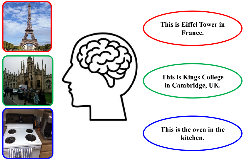
Figure 1: Humans’ efficient localization system. Humans encode places as landmarks in the memory in a self-supervised manner. These places could be famous buildings such as Eiffel Tower and Kings College or common objects such as ovens. As these landmarks are associated with unique locations, when seeing them, humans know where they are.

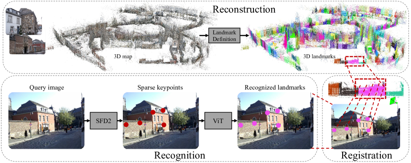
Figure 2: Overview of our framework. The reconstruction module recovers the 3D map from reference images and defines 3D landmarks hierarchically; the recognition module extracts sparse keypoints from the query image and predicts corresponding landmark labels with visual transformers; with recognized landmarks, the registration module performs landmark-wise 2D-3D matching to estimate the absolute pose of the query image (better view in color).

Visual localization aims to estimate the rotation and position of a given image captured in a known environment. As a fundamental computer vision task, visual localization is the key technique to various applications such as virtual/augmented reality (VR/AR), robotics, and autonomous driving. After several decades of exploration, many excellent methods have been proposed and can be roughly categorized as absolute pose regression (APR) [1, 2, 5, 3, 14, 4, 15], scene coordinate regression (SCR) [16, 6, 9, 17, 18], and hierarchical methods (HM) [12, 10, 11, 12]. APRs implicitly embed the map into high-level features and predict the 6DoF pose with multi-layer perceptions (MLPs); they are fast especially for large-scale scenes, but have limited accuracy due to implicit 3D information representation. Unlike APRs, SCRs regress 3D coordinates for all pixels directly and estimate the pose with PnP [19] and RANSAC [20]. Despite the high accuracy in indoor environments, SCRs are hard to scale up to outdoor large-scale scenes. Instead of predicting 3D coordinates directly, HMs adopt global features [21, 22, 23] to search reference images in the database and then build correspondences between keypoints extracted from query and reference images. These 2D-2D matches are lifted to 2D-3D matches and used for absolute pose estimation with PnP [19] and RANSAC [20] as SCRs. Regardless of the outstanding accuracy and adaptability in large-scale scenes, HMs have high storage cost for global and local 2D descriptors of reference images and high time cost of global reference search and exhaustive 2D-2D matching especially when graph-based matchers [24, 25, 26, 27] are employed. In Table I, we list advantages and disadvantages of APRs, SCRs and HMs and want to ask:

Can we find an efficient and accurate solution to visual large-scale localization?

We take the inspiration from humans’ localization system. Humans localize themselves quickly by recognizing certain objects and their spatial relationships, as shown in Fig. 1. For example, The Eiffel Tower tells that we are in Pairs; the Kings College reveals that we are at the center of Cambridge city in UK; the oven implies we are in the kitchen. When uncertain about the recognition results, we align detailed structures of objects with those in our memory for verification. These techniques, if used for visual localization task, could significantly improve the efficiency especially in large-scale environments. However, it is not easy to achieve this because of two major challenges. The first one is how to define landmarks in the real world. Some previous works explore this by defining landmarks on object instances, e.g., building facades [11, 8]. Despite their promising performance in certain scenes, these methods can not be extended to any places like humans’ recognition system. Instead, we seek from the 3D map which contains all places in the environment and adopt a hierarchical clustering strategy to define landmarks on 3D points directly. This allows us to make any place a landmark automatically without any laborious labeling and thus solve the first challenge.

The second challenge is how to recognize a large number of landmarks efficiently. For example, the prediction layer outputs features with 512 Megabytes to recognize 512 landmarks for an image with size of $512\times 512$, impairing the efficiency especially on edge devices with limited computational resources. To solve this problem, we propose to recognize landmarks of sparse keypoints as opposed dense pixels. Sparse keypoints [28, 29, 30, 31, 32, 33] such as corners and their spatial relationships effectively reveal the structure of objects [34, 35] and hence can be used to replace dense but redundant pixels for recognition. Moreover, these keypoints are sparse tokens naturally, enabling us to leverage the more powerful transformers [36] for recognition.

In this paper, we propose the place recognition anywhere model (PRAM) for visual localization, as shown in Fig. 2. We first use the local feature method SFD2 [29] to extract sparse keypoints for 3D reconstruction; then we perform hierarchical clustering on reconstructed 3D points to define landmarks automatically in a self-supervised manner; finally, sparse keypoints along with their spatial relationships are used as tokens to be fed into a transformer-based recognition module to recognize landmark labels. At test time, sparse keypoints and their predicted landmarks are further used for fast semantic-aware registration between 2D keypoints and 3D points in the map for pose estimation.

Compared with prior frameworks [1, 3, 6, 10], PRAM has many advantages. (1) By recognizing landmarks, PRAM determines the coarse location with constant time and memory complexity as opposed to reference search with global descriptors, improving both the time and memory efficiency. (2) With predicted landmark labels, PRAM filters potential outlier keypoints which don’t have corresponding 3D points in the map to avoid redundant computation. Note that if a 2D keypoint is an inlier or outlier is and only is determined by if it has corresponding 3D point in the map. Manual definitions from previous works [13, 11] such as, keypoints from buildings are inliers, those from trees not, don’t generalize well. (3) Predicted landmarks allow the registration module to perform fast semantic-aware 2D-3D registration instead of lifting 2D-2D matches to 2D-3D matches in HMs [10, 11]. This further improves the time efficiency because a large amount of redundant 2D descriptors associated with reference images are discarded. (4) PRAM is flexible to be extended to multi-modality localization. Recognition makes localization a high-level perception task rather than a classic low-level task; any other signals such as GPS, texts, voices can be encoded as additional tokens to join keypoints for recognition enhancement. (5) Other inspirations from PRAM such as large-scale scene coordinate regression, robust keypoints selection for localization and map sparsification and so on will be discussed in Sec. 6 as open problems.

Our contributions are concluded as follows:

• We propose a new localization framework, called PRAM, which allows us to do localization anywhere efficiently.

• We comprehensively analyze the accuracy and efficiency of APRs, SCRs, HMs and PRAM. Results demonstrate that PRAM outperforms APRs and SCRs in terms of accuracy in large-scale scenes and gives higher time and memory efficiency than HMs.

• PRAM opens a new direction for efficient and accurate large-scale localization such as muti-modality localization, sparse scene coordinate regression, map sparsification and so on.

Our experiments on indoor 7Scenes [37], 12Scenes [38] datasets and outdoor CambridgeLandmarks [1] and Aachen [39] datasets demonstrate that PRAM is $50\times$ smaller and $2.4\times$ faster than previous state-of-the-art HMs [10, 11]. The rest the paper is organized as follows. We discuss related works in Sec. 2 and introduce PRAM in detail in Sec. 3. We evaluate our method in Sec. 4 and Sec. 5. We discuss potential insights of our framework for visual localization in Sec. 6 and conclude the paper in Sec. 7.

2 Related work

In this section, we discuss related works of previous localization methods and their differences with PRAM.

Visual localization. Visual localization methods can be roughly categorized as absolute pose regression (APR), scene coordinate regression (SCR), and hierarchical methods (HM). APRs encode query images as pose features and regress the pose with an MLP, as shown in Fig. 3. Posenet [1] is the first work implementing this idea. Due to its simplicity, high memory and time efficiency in large-scale scenes, a lot of variants have been proposed by introducing geometric loss [2], multi-view constraints [4, 5, 3, 40, 41, 42], view synthesis [43], feature selection [14, 41], pose refinement [15], and generation of additional training data [44]. However, their accuracy is still limited because of the retrieval nature of APRs [45].

SCRs first regress 3D coordinates for each pixel in the query image and then estimate the pose with PnP [19] and RANSAC [20], as shown in Fig. 3. Initially, this is achieved via random forest with RGBD data as input [16]. Later on, DSAC [6] and its variants [18, 7] extend it to RGB input and replace random forest with CNNs. More recently, sparse regression [46], hierarchical prediction [17], the separation of backbone and prediction head [9], to name a few, are introduced for better accuracy and training efficiency. SCRs compress the map into a compact network and give very accurate poses in small scenes such as indoor 7Scenes [37] and 12Scenes [38]. However, they have limited accuracy in large-scale scenes such as CambridgeLandmarks [1] and Aachen dataset [39] because of the challenging pixel-wise recognition.

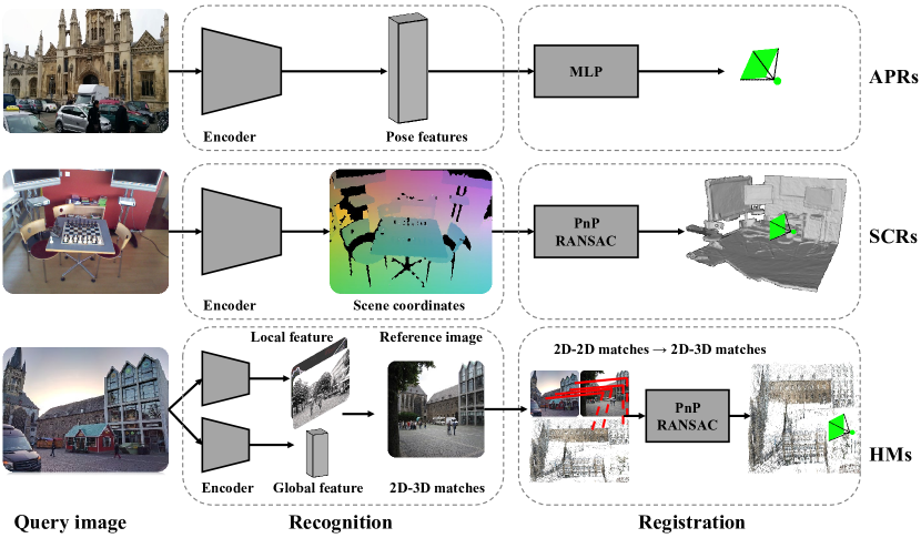
Figure 3: Frameworks of APRs, SCRs, and HMs. APRs [1, 5, 3, 4, 45] recognize the pose features and compute pose with an MLP as registration; SCRs [6, 18, 15] recognize dense pixel-wise coordinates and estimate the pose with PnP+RANSAC [19, 20] as registration; HMs [10, 11] perform recognition with global and local features matching and recover the pose with PnP+RANSAC [19, 20] as SCRs.

HMs [10, 11] estimate the pose of a query image by first finding reference images in the database, then building 2D-2D matches between keypoints in query and reference images, and finally computing the pose from associated 2D-3D matches lifted from 2D-2D ones with PnP [19] and RANSAC [20]. Traditionally, handcrafted SIFT [30] or ORB [31] features along with BoWs [47, 48] are widely used for the first two steps [12]. As handcrafted features are sensitive to illumination and seasonal changes, learned local features, e.g., Lift [33], SuperPoint (SP) [28], SFD2 [29] and global features, e.g., NetVLAD (NV) [21], GeM  [23] are mainly used. To further improve the accuracy, graph-based matchers, e.g., SuperGlue (SG) [24], SGMNet [26], IMP [25] are proposed to replace nearest matching for better matching quality. Nowadays, the combination of SP+NV+SG [28, 21, 24] has set the new state-of-art on public datasets [37, 38, 1, 39]. Despite the outstanding accuracy, HMs need to store a large amount of global and local features to build 2D-2D correspondences, impairing the memory efficiency. The exhaustive 2D-2D matching further degrades the time efficiency.

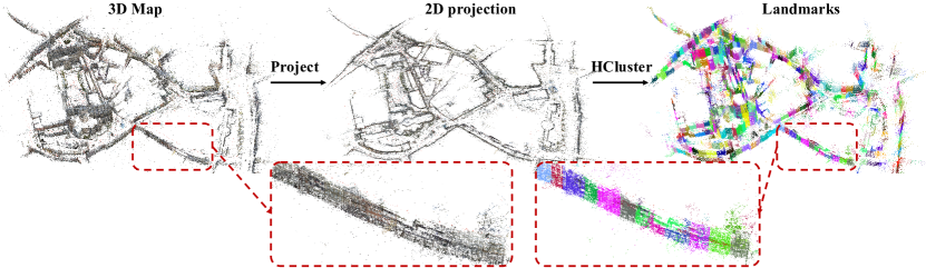
Figure 4: Landmark definition. The 3D points in the map are first projected to the ground plane as 2D projections. Then we employ a hierarchical approach to perform clustering on 2D projections based on spatial connections. Compared with reference images, the landmark map represents the large-scale Aachen city [39] in compact way with 512 landmarks (better view in color and zoom in).

Our PRAM also uses explicit sparse keypoints for 2D-3D matching as HMs, but PRAM is essentially different from HMs. First, the recognition module recognizes landmarks of places for coarse localization instead of performing global reference search with global features, therefore, PRAM is faster and more memory-efficient. Besides, with predicted landmarks as guidance, PRAM is able to build 2D-3D matches directly as opposed to lifting 2D-2D matches to 2D-3D matches. This further reduces the time and memory cost caused by exhaustive matching and redundant 2D descriptors, respectively.

As shown in Fig. 3, APRs, SCRs, and HMs can be viewed as special cases of recognition-registration combination in PRAM. APRs recognize the relationships between query and reference image features and then register the query image with a MLP for feature interpolation; Taking each 3D point as a landmark, SCRs recognize each pixel and recover the pose through PnP and RANSAC as registration; HMs recognize the query image by retrieval and perform registration via PnP and RANSAC as well. The key to visual localization is building 2D-3D matches efficiently and accurately, so the recognition will play a more significant role of localization in the future. By defining landmarks in the map and taking sparse keypoints as tokens, PRAM provides a wider space for making recognition efficient and accurate.

Visual semantic localization. Semantics compared to pixels are more robust to appearance changes, therefore researchers have tried almost all efforts to apply semantics for localization in the past decades. Most of these methods [13, 49, 50, 51, 52, 53] utilize explicit semantic labels predicted by segmentation networks [54, 55] to filter unstable keypoints and semantic-inconsistency matches. However, improvements are limited due to the following reasons. (1) Sparse keypoints detected from object boundaries have large segmentation uncertainties. (2) Segmentation results of images under challenging conditions (e.g., low-illumination) contain large errors [29]. (3) The manually defined strategy of filtering keypoints according to object classes has low generalization ability. For example, trees are useful for short-term localization [56, 57, 58] but useless for long-term localization [11, 13, 12]; trees can be used for place recognition, but may cause fine localization errors.

More recently, some of the aforementioned problems are solved. SFD2 [29] embeds semantics into the detector and descriptor implicitly and extracts semantic-aware features directly. The implicit embedding of semantics avoids semantic uncertainties of explicit labels at test time. However, these semantics can hardly be used for global place recognition. Instead, some works use building facades as a global instances for coordinate regression [8, 59] and fast reference image search [11]. But, these global instances defined only on building facades can hardly be applied to places without building facades such as indoor scenes. In short, although semantics have great potential to improve localization performance, segmentation errors due to low illumination, uncertainties from object boundaries, additional cost of segmentation networks, and low generalization ability in indoor and outdoor scenes degrade the gains of using semantics.

Different with aforementioned approaches, our landmarks defined in 3D map are beyond common semantics and can be used for both global place recognition and local matching in any places. Besides, landmark labels for points are defined in the map as opposed on objects, so there is no problem of uncertainties from object boundaries. Moreover, if a keypoint is an inlier or outlier is determined by whether it has a corresponding 3D point the map. The is embedded in the recognition module during the training process and has nothing to do with object labels. Therefore, PRAM generalizes well.

3 Method

In this section, we introduce our framework of place recognition anywhere model (PRAM) in detail. We first describe the map-centric landmark definition strategy and the structure of 3D map used for localization in Sec. 3.1 and Sec. 3.2, respectively. Then we provide details of recognizing landmarks with sparse keypoints in Sec. 3.3 and usage of predicted landmarks for localization in Sec. 3.4.

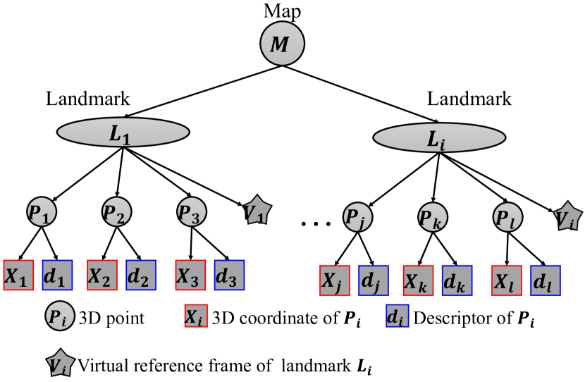
Figure 5: The structure of landmark map. A 3D map $\mathcal{M}$ is represented by a number of landmarks $\mathcal{L}=\{L_{1},...,L_{i}\}$. Each landmark $L$ contains several 3D points $\mathcal{P}=\{P_{1},...,P_{k}\}$ and a virtual reference frame $V$. Each 3D point $P$ consists of its 3D coordinate $X\in R^{3}$ and descriptor $\mathbf{d}\in R^{128}$.

3.1 Map-centric landmark definition

3D reconstruction. We reconstruct a 3D map represented by 3D points $\mathcal{X}=\{X_{1},...,X_{n}\}$ of the scene from images with current state-of-the-art 3D reconstruction library Colmap [60]. Instead of using handcrafted features [30, 31] and nearest matching, we adopt deep local feature SFD2 [29] and graph-based matcher IMP [25] to extract sparse keypoints and build correspondences, respectively. SFD2 [29] embeds semantics into features implicitly and is more robust appearance changes for long-term localization; IMP [25] gives better performance and runs faster than prior matchers [24, 26, 27]. Note that other deep features [28, 61, 32, 62] and matchers [24, 26, 27] can also be used in our framework. Each image $I\in R^{h\times w\times 3}$ ($h$ and $w$ are the height and width) is first fed into SFD2 network to extract $N$ sparse keypoints represented as $\{p:=(u,v,s,\mathbf{d}^{2D})\}$ where $(u,v)$ is the 2D coordinate, $s$ is the confidence of being a keypoint $p$, and $\mathbf{d}^{2D}$ is the descriptor. We employ the default setup of SFD2 to retain no more than 4k keypoints with scores over $0.005$ for each image in both the reconstruction and localization processes.

Due to insufficient observations and wrong matches, outlier 3D points exist in the map especially for outdoor scenes, impairing the map quality. To handle this, we only keep 3D points which are spatially consistent with their neighbors, as $\{X|V(X,\lambda_{n})\leq\lambda_{v}\}$ where $V(X,\lambda_{n})$ computes the covariance of a 3D point $X$ with its $\lambda_{n}$ nearest neighbors and $\lambda_{v}$ is the threshold. $\lambda_{n}$ and $\lambda_{v}$ are set to 20 and 0.2 in all of our experiments.

Landmark generation. We define landmarks on the 3D map directly in a self-supervised manner because the nature of localization is to find 2D-3D point-wise correspondences between query images and the map. In particular, we perform hierarchical clustering by merging 3D points from bottom to up according to their spatial distances. As most objects in real world such as bookshelf, table, tree and building facade are vertical to the ground, we project each 3D point $X$ to the 2D ground plane and then perform clustering on their 2D projections, allowing us to better maintain the completeness of objects particularly in outdoor environments. This whole process is as:

$$X^{2D} =\begin{bmatrix}1&0&0\\ 0&1&0\end{bmatrix}X,$$ (1)

$$\{L_{i},...,L_{k}\} =f_{hcluster}(\{X^{2D}_{i},...,X^{2D}_{k}\},\lambda_{l}).$$ (2)

$f_{hcluster}$ is the function performing hierarchical clustering on projected point set $\{X^{2D}_{1},...,X^{2D}_{k}\}$. As with BIRCH [63], we employ the same metric defined on clustering feature to decide if a new point should be merged into an existing leaf or taken as a new leaf. We refer BIRCH [63] for more details about the clustering process. The merging process stops until reaching the given number of landmarks $\lambda_{l}$ which is a hyper-parameter. Compared to K-means [64] clustering, $f_{hcluster}$ iteratively reduces and clusters through hierarchy clustering feature tree and works better for large-scale data with low dimensions. Moreover, some objects are still split into different landmarks even if with the spatial constraints. The hierarchical manner in $f_{hcluster}$ is flexible to accept other information such as object consistency provided by SAM [65] to mitigate the problem. Currently, we find results of SAM are noisy especially for outdoor scenes, leading to conflicts of the same objects between multi-view observations. In the future, we will reduce the noise of SAM results and add object-level constraints to $f_{hcluster}$.

Previous frameworks [10, 11] prefer to use reference images in the database, so they have to store global and local descriptors of reference images, resulting in huge memory cost. Additionally, reference images do not contain scale information of the scene and it may take hundreds even thousands of redundant images to represent an indoor room. The 3D map, however, has the absolute scale of the scene and avoids the redundancy. Therefore, we adopt a map-centric strategy to define landmarks directly on the 3D map as opposed to images.

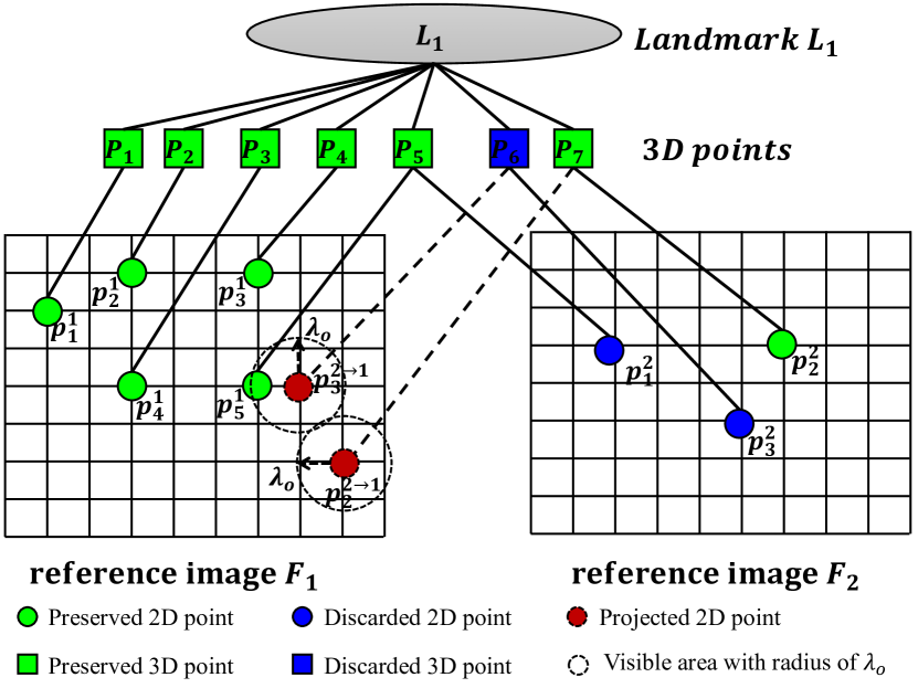
Figure 6: Landmark-wise point pruning. We take landmark $L_{1}$ with 3D points of $\{P_{1},...,P_{7}\}$ and two reference images $F_{1},F_{2}$ for example. We first retain points $P_{1:5}$ as they can be observed by $F_{1}$. As $P_{5}$ is already observed by $F_{1}$ as $p^{1}_{5}$, its observation on $F_{2}$ as $p^{2}_{1}$ is removed. The 2D projection $p^{2->1}_{3}$ of $P_{6}$ observed by $p^{2}_{3}$ has a keypoint $p^{1}_{5}$ within a circle visible area of radius of $\lambda_{o}$, so $P_{6}$ is removed from landmark $L_{1}$ and its 2D observation $p^{2}_{3}$ is also removed from $F_{2}$. The 2D projection $p^{2->1}_{2}$ of $P_{7}$ observed by $p^{2}_{2}$ on $F_{2}$ has no candidates within circle of radius $\lambda_{o}$, so $P_{7}$ and $p^{2}_{2}$ are retained.

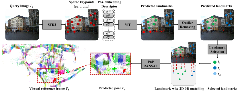
Figure 7: Pipeline of localization by sparse recognition. For a given query image, we first extract sparse keypoints with SFD2 [29] model. Then, descriptors and position embeddings of these keypoints are fed into a visual transformer for landmark prediction. Next, outliers with predicted labels of 0 are discarded for efficient registration. The left keypoints and their labels are used for selection of candidate landmarks for registration. For each selected candidate landmark, we perform landmark-wise matching between the query and corresponding virtual reference frame. Finally, PnP [19] and RANSAC [20] are used to estimate the absolute pose.

3.2 Map representation

With reconstructed 3D points $\{X\}$ and generated landmarks $\{L\}$, we name the map as $\mathcal{M}$ and reorganize its structure to fit our PRAM localization framework.

Structure of Map. As shown in Fig. 5, the map $\mathcal{M}$ is represented by a number of landmarks $\{L_{1},...,L_{k}\}$; each landmark $L_{i}$ contains some 3D points $\{P_{1},...,P_{j}\}$ and a virtual reference image (VRF) $V_{i}$; each 3D point $P_{i}$ is represented by its 3D coordinates $X_{i}$, landmark $L_{i}$, and 3D descriptor $\mathbf{d}_{i}$.

3D Descriptor. Each 3D point $P_{i}$ is assigned with a 3D descriptor to build 2D-3D matches between query images and the map for registration. In order to mitigate the domain differences between 2D and 3D points, we select 3D descriptors carefully for each 3D point $P_{i}$ from its 2D observations in the reconstruction process, as:

$$\mathbf{d}_{i}=\operatorname*{argmin}_{\mathbf{d}}f_{md}(\mathbf{d},\mathbf{d}^{2D}_{1},...,\mathbf{d}^{2D}_{j}),\mathbf{d}\in\{\mathbf{d}^{2D}_{1},...,\mathbf{d}^{2D}_{j}\}.$$ (3)

For point $P_{i}$, its descriptor $\mathbf{d}_{i}$ is the 2D descriptor which has the smallest median distance computed by $f_{md}$ to all other 2D descriptors $\{\mathbf{d}^{2D}_{1},...,\mathbf{d}^{2D}_{j}\}$ of keypoints observing $P_{i}$ on reference images. Median distance has better statistical robustness and has been proved effective to appearance changes [56] especially when query and reference images are captured at different times.

Virtual reference frame (VRF). We assign each landmark $L_{i}$ a virtual reference frame (VRF) $V_{i}$ for two reasons. First of all, the pose of a VRF can be used as an approximation of the landmark. In the localization process, such approximation can be used as the coarse location of the query image. Besides, VRFs allow our model to perform 2D-2D matching between query images and VRFs instead of direct 2D-3D matching, mitigating the domain differences between 2D and 3D points. Note that VRFs are different from reference images used in HMs [11, 10] as VRFs don’t contain any global or local descriptors. For the two aforementioned reasons, the VRF $V_{i}$ assigned for landmark $L_{i}$ should satisfy the requirement that $V_{i}$ observes the majority part of 3D points belonging to $L_{i}$. Therefore, we choose $V_{i}$ for landmark $L_{i}$ as:

$$V_{i}=\operatorname*{argmax}_{F}f_{obs}(F,L_{i}),f_{obs}=\frac{|\{X_{i}|X_{i}\in\mathcal{X}_{F}\cap\mathcal{X}_{i}\}|}{|\{X_{i}|X_{i}\in\mathcal{X}_{i}\}|}.$$ (4)

$V_{i}$ is the reference image which observes the most number of 3D points belonging to landmark $L_{i}$. $f_{obs}$ computes the ratio of the number of observed points $|\{X_{i}|X_{i}\in\mathcal{X}_{F}\cap\mathcal{X}_{i}\}|$ and the total number of points $|\{X_{i}|X_{i}\in\mathcal{X}_{i}\}|$ in $L_{i}$. Each VRF $V_{i}$ has the intrinsic ${K_{i}}$ and extrinsic parameters $T_{i}$. These virtual reference images will be used in the localization process as discussed in Sec. 3.4.

Adaptive landmark-wise pruning. Landmarks provide strong priors for 2D-3D matching between query images and the map, so it is unnecessary for each landmark to preserve a large number of usually redundant points. Therefore, we remove these redundant 3D points in a greedy manner for each landmark independently.

Initially, let $F_{1},...,F_{n}$ and $\mathcal{X}_{F_{1}},...,\mathcal{X}_{F_{n}}$ be reference images and corresponding observed 3D points in the landmark $L_{i}$. $F_{1}$ to $F_{n}$ are sorted in a descending order according to their numbers of observations ($|\mathcal{X}_{F_{1}}|\geq|\mathcal{X}_{F_{2}}|\geq...\geq\mathcal{X}_{F_{n}}$). According to Eq 4, intrinsic and extrinsic parameters of $F_{1}$ are used to construct the VRF of $L_{i}$. For the first iteration, we choose $F_{1}$ as the reference image and initialize preserved keypoints for $F1$ as $\mathcal{X}^{p}_{F_{1}}=\mathcal{X}_{F_{1}}$. Then, we remove repetitive points on $F_{2}$ which can be observed by $F_{1}$ as:

$$\mathcal{X}^{p}_{F_{2}}=\mathcal{X}_{F_{2}}-f_{covis}(F_{1},F_{2},\mathcal{X}_{F_{1}},\mathcal{X}_{F_{2}},\lambda_{o}).$$ (5)

Any point on $F_{2}$ is discarded as long as its reprojection distance to any points on $F_{1}$ is smaller than $\lambda_{o}$, as shown in Fig. 6. This strategy guarantees the localization accuracy after removing redundant points due high overlap. $\mathcal{X}^{p}_{F_{2}}$ is the set of kept points on $F_{2}$ and $f_{covis}$ computes the covisible points within the threshold of $\lambda_{o}$. For the i$th$ iteration, the updating process is as:

$$\mathcal{X}^{p}_{F_{i+1}}=\mathcal{X}_{F_{i+1}}-f_{covis}(F_{1:i},F_{i+1},\mathcal{X}^{p}_{F_{1}:F_{i}},\mathcal{X}_{F_{i+1}},\lambda_{o}).$$ (6)

This process is repeated until processed images have over 80% points $(\frac{|\mathcal{X}_{F_{1}}\cup...\cup\mathcal{X}_{F_{i}}|}{|\mathcal{X}_{F_{1}}\cup...\cup\mathcal{X}_{F_{n}}|})$. Finally, we collect preserved points from all processed images as $\mathcal{X}^{p}_{F_{1}}\cup...\cup\mathcal{X}^{p}_{F_{n}}$ to replace the original full point set $\mathcal{X}_{F_{1}}\cup...\cup\mathcal{X}_{F_{n}}$ as points associated to landmark $L_{i}$. Compared with previous methods solving a K-cover [66] or quadratic programming [67] problem for the whole map, this strategy can simply applied to each landmark independently.

Algorithm 1 Localization by sparse recognition

1:Step1: given sorted predicted landmarks $\mathcal{L}^{{}^{\prime\prime}}=\{l_{1},...,l_{n}\}$ and corresponding keypoints $\{\mathcal{P}^{{}^{\prime\prime}}_{ql_{1}},...,\mathcal{P}^{{}^{\prime\prime}}_{ql_{n}}\}$ in $\mathcal{P}^{{}^{\prime\prime}}_{q}$

2:for $l$ in $\mathcal{L}^{{}^{\prime\prime}}$ do

3:     $V_{l},\mathcal{P}_{l}\leftarrow f_{retrieve}(\mathcal{M},l)$ $\triangleright$ retrieve VRF and 3D points for landmark $l$ from 3D map $\mathcal{M}$

4:     $\mathcal{P}^{2D}_{l}=f_{proj}(\mathcal{P}_{l},V_{l})$ $\triangleright$ project 3D keypoints to VRF

5:     $M_{l}=f_{sm}(\mathcal{P}^{{}^{\prime\prime}}_{ql},\mathcal{P}^{2D}_{l})$ $\triangleright$ semantic-aware matching for landmark $l$

6:     $T_{l},n_{l}=f_{epnp+ransac}(M_{l})$ $\triangleright$ estimate the pose $T_{l}$ and number of inliers $n_{l}$ with EPnP + RANSAC

7:     if $n_{l}\geq\lambda_{i}$ then $\triangleright$ successfully find a good pose with sufficient inliers

8:         $T^{*}\leftarrow T_{l},V^{*}\leftarrow V_{l}$ $\triangleright$ return the pose and VRF

9:         break

10:     end if

11:end for

12:Step 2 (optional): refine the initial pose $T^{*}$ with more 3D points

13:$\mathcal{X}^{*}=f_{covis}(\mathcal{M},V^{*})$ $\triangleright$ find more 3D points with covisibility

14:$M^{*}=f_{geo}(\mathcal{P}^{{}^{\prime\prime}}_{q},\mathcal{L}^{{}^{\prime\prime}},T^{*})$ $\triangleright$ find more matches with initial pose

15:$T_{q}=f_{refine}(M^{*},T^{*})$ $\triangleright$ refine the pose

3.3 Sparse recognition

After each 3D point $P$ is associated with a landmark label $L$, 2D keypoints $p$ observing $P$ is automatically associated with the landmark label $L$. 2D keypoints without 3D correspondences due to non-successful triangulation or outlier filtering are assigned with label 0, indicating that these 2D keypoints have no corresponding 3D points in the map.

In the training process, to better utilize the spatial connections of extracted keypoints $p$, position embedding is employed by encoding $(u,v)$ into a high level position feature vector with position encoder $f_{pos}$. The position feature vector and original descriptor $\mathbf{d}^{2D}$ are fed into a visual transformer $f_{ViT}$ for landmark recognition. The whole process can be represented as:

$$\mathbf{d}^{{}^{\prime}}_{i} =\mathbf{d}^{2D}_{i}+f_{pos}(u_{i},v_{i}),$$ (7)

$$S_{1},S_{2},...,S_{m} =f_{ViT}(\mathbf{d}^{{}^{\prime}}_{1},\mathbf{d}^{{}^{\prime}}_{2},...,\mathbf{d}^{{}^{\prime}}_{m}),$$ (8)

$$Loss =-\frac{1}{m}\sum_{i=1}^{m}w(x_{i})\sum_{j=1}^{\lambda_{l}+1}S^{gt}_{ij}log(S_{ij}),$$ (9)

$S_{ij}$ and $S^{gt}_{ij}$ are predicted and ground-truth confidences of $p_{i}$ belonging to landmark $L_{j}$ after softmax. $\lambda_{l}$ is the total number of landmarks excluding 0. We adopt a weighted cross entropy loss with weight of $w_{i}$ to balance the valid and invalid keypoints. $w_{i}$ is set to $\frac{m_{0}}{m}$ if $L_{i}\neq 0$ otherwise $1-\frac{m_{0}}{m}$ ($m_{0}$ and $m$ are the number of keypoints with label 0 and the total number of keypoints, respectively).

We use all extracted keypoints from images for recognition in both training and testing processes because these keypoints extracted at different locations provide global context to support landmark recognition. For example, keypoints with correspondences (e.g., from buildings) in the map can be used for both recognition and registration; keypoints without correspondences (e.g., from trees) are also useful visual clues for recognition.

3.4 Localization by recognition

As shown in Fig. 7, in the localization process, given a query image $I_{q}$, we first extract sparse keypoints with SFD2 [29] denoted as $\mathcal{P}_{q}$ and then predict the landmark labels $\mathcal{L}_{q}$ and corresponding confidences $\mathcal{S}_{q}$ with $f_{ViT}$. In this section, we provide details of how to use predicted landmarks $\mathcal{L}_{q}$ and confidences $\mathcal{S}_{q}$ for localization.

Outlier removing. Extracted sparse keypoints generally contain a large number of keypoints without 3D correspondences in the map. These keypoints are useful for recognition, yet they are useless for registration. Fortunately, in the training process, these keypoints are assigned with label 0, so in the localization process, keypoint $X^{q}_{i}$ with confidence $S^{q}_{i}$ of being label 0 over than the threshold $\lambda_{s}$ can be easily identified and removed. $\lambda_{s}$ is set to 0.9 in our experiments. The left keypoints along with their landmarks and confidences are denoted as $\mathcal{P}^{{}^{\prime}}_{q}$, $\mathcal{L}^{{}^{\prime}}_{q}$ and $\mathcal{S}^{{}^{\prime}}_{q}$, respectively.

For outlier removing, we adopt only one universal metric that if a keypoint has a corresponding 3D point in the map. Compared with previous widely-used strategy of utilizing object labels as priors (e.g., keypoints from buildings are inliers, keypoints from trees are not) [11, 52, 13, 68], our method is simpler and generalizes well in any environments.

Landmark selection. A query image usually observes several landmarks in the map, as shown in Fig. 7. To accelerate the verification process, we sort recognized landmarks in $\mathcal{L}^{{}^{\prime}}_{q}$ in a descending order according to their mean confidence $\mathcal{S}^{{}^{\prime}}_{q}$ of belonging to a certain landmark. These sorted landmarks, corresponding confidences and keypoints are denoted as $\mathcal{L}^{{}^{\prime\prime}}_{q}$, $\mathcal{S}^{{}^{\prime\prime}}_{q}$ and $\mathcal{P}^{{}^{\prime\prime}}_{q}$, respectively. As keypoints with labels of being 0 are already removed, all keypoints in $\mathcal{X}^{{}^{\prime\prime}}_{q}$ can be used for verification.

Landmark-wise 2D-3D matching. For each label $l$ in $\mathcal{L}^{{}^{\prime\prime}}_{q}$, 2D keypoints $\mathcal{P}^{{}^{\prime\prime}}_{ql}$ and 3D points $\mathcal{P}_{l}$ belonging to label $l$ are used to build 2D-3D matches. In order to leverage the spatial information, we adopt the graph-based matcher IMP [25] to find 2D-3D matches. However, due to occlusions among 3D points and domain differences between 2D and 3D points, direct 2D-3D matching is not robust. Instead, we reproject 3D points $\mathcal{P}_{l}$ on the virtual reference frame $V_{l}$ of landmark $l$ as $\mathcal{P}^{2D}_{l}$, avoiding the occlusions and domain differences. We use the projected 2D coordinates and 3D descriptors as input to IMP. In this stage, as only keypoints with the same label are used for matching, our approach avoids exhaustive matching and reduces time cost significantly.

Registration. The 2D-3D matches are fed into the PnP [19] + RANSAC [20] to estimate the absolute pose $T_{q}\in R^{3\times 4}$ of the query image. If the number of inliers is over than $\lambda_{i}$, the verification is deemed success, otherwise the next candidate landmark in $\mathcal{L}^{*}_{q}$ is used until a successful pose is found or all $\lambda_{c}$ candidate landmarks are explored. The pose $T_{q}$ recovered from a single landmark may not be very precise due to insufficient matches, so we further refine the pose by finding more co-visible 2D-3D matches with the initially estimated pose $T_{q}$ as in [11]. The whole process is described by Algorithm 1.

TABLE II: Recognition results. For each dataset rather than a sub-scene in the dataset, we train a recognition model to recognize all landmarks in that dataset. We report the recognition precision of top@1 on 7Scenes[37] (S), 12Scenes [38] (T), CambridgeLandmarks [1] (C) and Aachen [39] (A) datasets. The number of scenes (#Scenes), landmarks (#Landmarks) and the average number of keypoints (#keypoints) are also included for reference.

Dataset	#Scenes	#Landmarks	#Keypoints	Precision@1
			day, night	day, night
S [37]	7	112	412.7, NA	80.0%, NA
T [38]	12	192	435.3, NA	95.0%, NA
C [1]	5	160	4087.8, NA	87.6%, NA
A [39]	1	512	3192.2, 3262.7	69.8%, 49.7%

TABLE III: Localization accuracy on 7Scenes [37] and 12Scenes [38] datasets. We report the median position ($cm$) and orientation ($\circ$) errors and localization precision with position and orientation errors within $5cm,5^{\circ}$. NA indicates values unavailable.

Group	Method	7Scenes	12Scenes
		$t(cm)/R(^{\circ})/Percent(5cm,5^{\circ}$)
APRs	LsG [5]	19 / 7.47 / NA	NA / NA / NA
	AtLoc [14]	20 / 7.6 / NA	NA / NA / NA
	PAEs [69]	19 / 7.5 / NA	NA / NA / NA
	LENS [44]	8 / 3.0 / NA	NA / NA / NA
	Posenet [1]	24 / 7.9 / 1.9	NA / NA / NA
	MapNet [4]	21 / 7.8 / 4.9	NA / NA / NA
	MS-Transformer [70]	18 / 7.3 / 4.1	NA / NA / NA
	GLNet [3]	19 / 6.3 / 7.8	NA / NA / NA
SCRs	VSNet [71]	2.4 / 0.8 / NA	NA / NA / NA
	PixLoc [72]	2.9 / 0.98 / NA	NA / NA / NA
	CAMNet [73]	4 / 1.69 / NA	NA / NA / NA
	SANet [74]	5.1 / 1.68 / NA	NA / NA / NA
	KFNet [75]	2.9 / 1.0 / NA	NA / NA / 98.9
	NeRF-loc [76]	2.3 / 1.3 / 89.5	NA / NA / NA
	SC-wLS [15]	7 / 1.5 / 43.2	NA / NA / NA
	DSAC* [18]	2.7 / 1.4 / 96.0	NA / NA / 99.6
	ACE [9]	2.5 / 1.3 / 97.1	1.0 / 0.4 / 99.9
	HSCNet [17]	3 / 0.9 / 84.8	0.1 / 0.5 / 99.3
HMs	AS [12]	NA / NA / 98.5	NA / NA / 99.8
	SP+SG [28, 24]	1.0 / 0.2 / 95.7	1.0 / 0.1 / 100
	SFD2+IMP [29, 25]	1.0 / 0.1 / 95.7	1.0 / 0.1 / 99.7
	Ours	1.0 / 0.3 / 97.3	1.0 / 0.1 / 97.8

TABLE IV: Localization accuracy on the CambridgeLandmarks dataset [1]. We report the median position (cm), orientation (^∘) errors and localization success ratio of pose errors within ($25cm,2^{\circ}$). NA indicates values unavailable.

Group	Method	Kings College	Great Court	Old Hospital	Shop Facade	St Marys Church	Average
		$t(cm)/R(^{\circ})/Percent(25cm,2^{\circ}$)
APRs	MapNet [4]	107 / 1.9 / NA	785 / 3.8 / NA	149 / 4.2 / NA	200 / 4.5 / NA	194 / 3.9 / NA	163 / 3.6 / NA
	PAEs [69]	90 / 1.5 / NA	NA / NA / NA	207 / 2.6 / NA	99 / 3.9 / NA	164 / 4.2 / NA	140 / 3.1 / NA
	LENS [44]	33 / 0.5 / NA	NA / NA / NA	44 / 0.9 / NA	27 / 1.6 / NA	53 / 1.6 / NA	39 / 1.2 / NA
	Posenet [1]	88 / 1.0 / 0	683 / 3.5 / 0	88 / 3.8 / 0	157 / 3.3 / 0	320 / 3.3 / 0	163 / 2.9 / 0
	MS-Transformer [70]	83 / 1.5 / 3.5	NA / NA / NA	181 / 2.4 / 2.2	86 / 3.1 / 4.9	162 / 4.0 / 0.4	128 / 2.8 / 2.8
	GLNet [3]	59 / 0.7 / 3.4	NA / NA / NA	50 / 2.9 / 3.6	190 / 3.3 / 7.9	188 / 2.8 / 0.6	122 / 2.4 / 3.9
SCRs	NeRF-loc [76]	7 / 0.2 / NA	25 / 0.1 / NA	18 / 0.4 / NA	11 / 0.2 / NA	4 / 0.2 / NA	13 / 0.2 / NA
	HSCNet [17]	18 / 0.3 / NA	28 / 0.2 / NA	19 / 0.3 / NA	6 / 0.3 / NA	9 / 0.3 / NA	16 / 0.3 / NA
	SC-WLS [15]	14 / 0.6 / 68.2	164 / 0.9 / 7.3	42 / 1.7 / 23.1	11 / 0.7 / 76.7	39 / 1.3 / 34.0	27 / 1.0 / 42.0
	DSAC* [18]	13 / 0.4 / 72.3	40 / 0.2 / 22.2	20 / 0.3 / 57.1	6 / 0.3 / 91.3	13 / 0.4 / 81.5	18 / 0.3 / 64.9
	ACE [9]	28 / 0.4 / 44.6	42 / 0.2 / 28.7	31 / 0.6 / 40.7	5 / 0.3 / 98.1	19 / 0.6 / 61.3	25 / 0.42 / 54.7
HMs	AS [12]	24 / 0.1 / NA	13 / 0.2 / NA	20 / 0.4 / NA	4 / 0.2 / NA	8 / 0.3 / NA	14 / 0.2 / NA
	PixLoc [72]	14 / 0.2 / NA	30 / 0.1 / NA	16 / 0.3 / NA	5 / 0.2 / NA	10 / 0.3 / NA	15 / 0.2 / NA
	SANet [74]	32 / 0.5 / NA	328 / 2.0 / NA	32 / 0.5 / NA	10 / 0.5 / NA	16 / 0.6 / NA	84 / 0.8 / NA
	DSM [77]	19 / 0.4 / NA	43 / 0.2 / NA	23 / 0.4 / NA	6 / 0.3 / NA	11 / 0.3 / NA	20 / 0.3 / NA
	SFD2+IMP [29, 25]	7 / 0.1 / 94.8	11 / 0.1 / 74.6	10 / 0.2 / 80.2	2 / 0.1 / 97.1	4 / 0.1 / 98.7	7 / 0.1 / 89.1
	SP+SG [28, 24]	7 / 0.1 / 94.5	12 / 0.1 / 74.7	9 / 0.2 / 81.9	2 / 0.1 / 97.1	4 / 0.1 / 98.7	7 / 0.1 / 89.4
	Ours	15 / 0.1 / 71.1	16 / 0.1 / 62.5	9 / 0.2 / 78.0	2 / 0.1 / 98.1	5 / 0.2 / 96.8	9 / 0.1 / 81.3

4 Experiment Setup

In this section, we first give more implementation details. Then, we introduce the datasets, metrics and baseline methods used for evaluation and comparison. More visualization of automatic landmark generation and localization by recognition on public and custom datasets are provided in the supplementary materials.

Implementation. We implement the recognition model $f_{ViT}$ with 15 multi-head attention layers on PyTorch [78]. The number of head and dimension of feature are set to 4 and 256. $f_{pos}$ is a 4-layer MLP with hidden dimension of 32, 64, 128 and 256. All models are trained with Adam optimizer [79] with batch size of 32 on the NVIDIA RTX 3090. We adopt SFD2 [29] to extract sparse keypoints and IMP [25] to build 2D-3D correspondences in the localization process. Hyper-parameter $\lambda_{o}$ is set to 25; $\lambda_{l}$ is set to 112, 192, 160, 512, $\lambda_{c}$ is set to 20, 20, 20, 50, and $\lambda_{i}$ is set to 64, 64, 128, 128 for 7Scenes [37], 12Scenes [38], CambridgeLandmarks [1] and Aachen [39] datasets.

Dataset. Our approach is evaluated on a variety of public indoor and outdoor datasets including 7Scenes [37], 12Scenes [38], CambridgeLandmarks  [1], and Aachen Day-Night [39] datasets. 7Scenes and 12Scenes are both indoor scenes with 7 and 12 individual rooms, respectively. Each room has the size of about $2m\times 2m\times 2m$. Due to small scale, almost all previous SCRs [15, 9] and HMs [10, 11] have reported excellent performance. CambridgeLandmarks dataset consists of 5 individual scenes captured at the center of Cambridge city. Each has an area size of about $20m\times 50m$ (for simplicity, we omit the height for outdoor scenes). Aachen dataset contains images captured at different seasons with various viewpoints in the Aachen city. It has an area size of about $3km\times 2km$, making the localization very challenging. The illumination and seasonal variations between query and reference images further increase the localization difficulty. Different with previous APRs [1, 2, 5, 3, 15, 14] and SCRs [6, 18, 9, 17] training a separate model for each scene, in our experiments, we take each dataset as a whole and train a single model to recognize all landmarks in each dataset. The number of landmarks for different datasets are demonstrated in Table II.

Metric. As with previous works [6, 80, 15, 11], for 7Scenes [37] and 12Scenes [38] datasets, we report median pose errors ($cm,^{\circ}$) and the success ratio of query images with pose errors within in ($5cm,5^{\circ}$). For CambridgeLandmarks [1], we report the median rotation and translation errors as well. Additionally, we provide the success ratio at the error threshold of ($0.25m,2^{\circ}$) as only median errors cannot reveal the real performance. For Aachen dataset, we use the official metric by reporting the success ratio of poses within error thresholds of ($0.25m,2^{\circ}$), ($0.5m,5^{\circ}$), and ($5m,10^{\circ}$), respectively. Besides, since we focus on both the accuracy and efficiency of localization, we also analyze the time and memory cost of previous and our systems.

Baseline. We compare our approach with previous state-of-the-art APRs [1, 3, 5, 14, 4, 70, 69, 44],SCRs [6, 18, 9, 17, 75, 81, 76, 73, 74, 15] and HMs [12, 82, 83, 32, 61, 10, 29, 50, 49, 13, 72]. Results of SFD2+IMP and SP+SG are from officially released source code with NetVLAD providing 20, 20, 20, 50 candidates on 7Scenes, 12Scenes, CambridgeLandmarks, and Aachen datasets, respectively. For other methods, results are from their paper or officially released source code.

5 Experiments

In this section, we analyze the recognition results, localization accuracy, map size, and running time in Sec. 5.1, Sec. 5.2, Sec. 5.3 and Sec. 5.4, respectively. We further conduct an ablation study to verify the efficacy of different components in our model in Sec. 5.5 and visualize qualitative results in Sec. 5.6.

5.1 Landmark recognition

As shown in Table II, for the evaluation of recognition performance, we report the average top@1 precision ($\frac{\#correct\quad keypoints}{\#all\quad keypoints}$) in each dataset for day and night images, separately. Since groundtruth poses of query images in Aachen dataset [39] are not publicly available, we use poses given by SFD2+IMP [29, 25] to generate pseudo groundtruth labels for sparse keypoints. Note that although SFD2+IMP [29, 25] achieves state-of-the-art accuracy on the Aachen dataset [39], estimated poses especially on night images are not perfect, therefore the groundtruth of recognition is not perfect, neither.

Table II shows that in indoor scenes such as 7Scenes and 12Scenes datasets [37, 38] consisting of 112 and 192 landmarks respectively, our model gives precision over 80% by using about 400 keypoints for each query image. We yield about 87.9% precision on CambridgeLandmarks [1] with about 4,000 keypoints as input. While for Aachen dataset [39], the precision degrades to 69.8% due to the large viewpoint changes on day images. Illumination changes and the missing night images for training further impair the performance, leading to the precision of 49.7% on night images. Although the top@1 precision of night images is not as high as that of day images, our strategy of retaining several candidate landmarks for verification as introduced in Sec. 3.4 increases the localization success ratio. In the future, more data augmentation could be leveraged to improve the recognition performance on images with large view-point and illumination changes.

TABLE V: Map size. We show the number of number of reference image (#Ref. images), 3D points (#3D points) and the local descriptor (local desc.), global descriptor (global desc.), 3D map size and the total size at test time. The datasets include 7Scenes (S) [37], 12Scenes (T) [38], CambridgeLandmarks (C) [1] and Aachen (A) [39].

Dataset	Method	# Ref. images	#3D point (M)	local desc. (G)	global desc. (G)	Map size (G)	Total size (G)
S	Posenet [1]	0	0	0	0	0.33	0.33
	GLNet [3]	0	0	0	0	0.59	0.59
	DSAC* [18]	0	0	0	0	0.03	0.03
	ACE [9]	0	0	0	0	0.004	0.004
	SP+SG [28, 24, 21]	26,000	0.66	14.6	0.79	0.50	15.90
	SFD2+IMP [29, 25]	26,000	0.44	5.78	0.79	0.39	6.96
	Ours	0	0.05	0	0	0.03	0.03
T	Posenet [1]	0	0	0	0	0.56	0.56
	GLNet [3]	0	0	0	0	1.00	1.00
	DSAC* [18]	0	0	0	0	0.03	0.03
	ACE [9]	0	0	0	0	0.004	0.004
	SP+SG [28, 24, 21]	16,989	0.84	11.62	0.52	0.43	12.57
	SFD2+IMP [29, 25]	16,989	0.59	4.45	0.52	0.33	5.30
	Ours	0	0.15	0	0	0.08	0.08
C	Posenet [1]	0	0	0	0	0.23	0.23
	GLNet [3]	0	0	0	0	0.42	0.42
	DSAC* [18]	0	0	0	0	0.14	0.14
	ACE [9]	0	0	0	0	0.02	0.02
	SP+SG [28, 24, 21]	5,365	1.65	10.81	0.16	0.63	11.60
	SFD2+IMP [29, 25]	5,365	1.55	5.31	0.16	0.63	6.1
	Ours	0	0.4	0	0	0.22	0.22
A	SP+SG [28, 24, 21]	6,697	2.15	13.83	0.20	0.72	14.76
	SFD2+IMP [29, 25]	6,697	2.21	7.21	0.2	0.80	8.17
	Ours	0	1.33	0	0	0.72	0.72

TABLE VI: Results on Aachen dataset [39, 84]. We report the pose accuracy at error thresholds of $(0.25m,2^{\circ})$, $(0.5m,5^{\circ})$ and $(5m,10^{\circ})$. * indicates methods using semantics for localization.

Group	Method	Day	Night
		$(0.25m,2^{\circ})/(0.5m,5^{\circ})/(5m,10^{\circ})$
SCRs	ESAC [85]	42.6 / 59.6 / 75.5	3.1 / 9.2 / 11.2
	HSCNet [17]	71.1 / 81.9 / 91.7	32.7 / 43.9 / 65.3
	NeuMap [86]	80.8 / 90.9 / 95.6	48.0 / 67.3 / 87.8
HMs	SSM* [50]	71.8 / 91.5 / 96.8	58.2 / 76.5 / 90.8
	VLM* [51]	62.4 / 71.8 / 79.9	35.7 / 44.9 / 54.1
	SMC* [13]	52.3 / 80.0 / 94.3	29.6 / 40.8 / 56.1
	LBR* [11]	88.3 / 95.6 / 98.8	84.7 / 93.9 / 100.0
	SFD2* [29]	88.2 / 96.0 / 98.7	87.8 / 94.9 / 100.0
	AS  [12]	85.3 / 92.2 / 97.9	39.8 / 49.0 / 64.3
	CSL [82]	52.3 / 80.0 / 94.3	29.6 / 40.8 / 56.1
	CPF [87]	76.7 / 88.6 / 95.8	33.7 / 48.0 / 62.2
	SceneSqqueezer [88]	75.5 / 89.7 / 96.2	50.0 / 67.3 / 78.6
	SP [28]	80.5 / 87.4 / 94.2	42.9 / 62.2 / 76.5
	R2D2 [32]	NA / NA / NA	76.5 / 90.8 / 100.0
	ASLFeat [89]	NA / NA / NA	81.6 / 87.8 / 100.0
	D2Net [61]	84.8 / 92.6 / 97.5	84.7 / 90.8 / 96.9
	SP+SG [28, 24]	89.6 / 95.4 / 98.8	86.7 / 93.9 / 100.0
	SFD2+IMP [29, 25]	89.7 / 96.5 / 98.9	84.7 / 94.9 / 100.0
	Ours	82.5 / 90.9 / 96.7	77.6 / 87.8 / 94.9

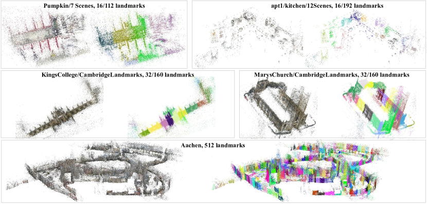
Figure 8: 3D map and landmarks. We visualize 3D map and landmarks in indoor (pumpkin in 7Scenes [37], apt1/kitchen in 12Scenes [38]), outdoor (Kings College and Marys Church in CambridgeLandmarks [1]) and city-scale scenes (Aachen [39]). We take each dataset as a whole, so the visualized landmarks are only from example scenes. The number of landmarks in example scenes and the total number of landmarks in the dataset are also included.

5.2 Pose estimation

7Scenes (S) and 12Scenes (T). Table III shows median position and orientation errors and success ratio at the error threshold of ($5cm,5^{\circ}$). APRs have the largest position and orientation errors due to implicit 3D information embedding and their similar behavior to image retrieval [45]. Among APRs [1, 69, 70, 3], GLNet [3] uses graph-based knowledge propagation for multi-view input images and gives the highest success ratio of 3.9 on average, yet it is not satisfying compared to SCRs and HMs.

SCRs achieve excellent performance on both 7Scenes and 12Scenes datasets with median position ($\approx 3cm$) and orientation ($\approx 1^{\circ}$) errors about 7$\times$ smaller than APRs ($\approx 20cm,7^{\circ}$). The outstanding performance of SCRs (ACE [9] achieves 97.1% and 99.9% pose accuracy on 7Scenes [37] and 12Scenes [38] datasets) come from their powerful coordinate regression ability in small scenes. Note that each scene in 7Scenes [37] and 12Scenes [38] datasets has the size of only $2m\times 2m\times 2m$ and SCRs train a model for each scene separately. Table IV demonstrates their limited accuracy on large-scale datasets [1, 39].

HMs obtain close accuracy to SCRs by performing sparse matching. Among HMs, AS  [12] (98.5% and 99.8%) works slightly better than SP+SG [28, 24] (95.7% and 100%) and SFD2+IMP  [29, 25] (95.7% and 99.7%) because AS extracts multi-scale SIFT [30] as local features which are slightly robust to areas with similar structures (e.g., stairs in 7Scenes) than single-scale corners used by SP [28] and SFD2 [29].

Our method ($\approx 1cm,0.3^{\circ}$) gives close performance to SP+SG [28, 24] ($\approx 1cm,0.1^{\circ}$) and SFD2+IMP[29, 25] ($\approx 1cm,0.1^{\circ}$) in terms of median errors. The better performance of our model on 7Scenes comes from the semantic-wise matching which is more robust to similar structures (e.g., stairs in 7Scenes). Our model reports slightly worse accuracy on 12Scenes [38] (97.8%) because of insufficient SFD2 features for recognition and 2D-3D matching in textureless regions (e.g., office2/5a in 12Scenes). SFD2+IMP solves this problem by utilizing 20 candidate images to build correspondences, so it works better.

CambridgeLandmarks (C). In Table IV, we show the localization results on CambridgeLandmarks [1] in terms of median position (cm) and orientation errors (^∘) and the pose accuracy at the error threshold of ($25cm,2^{\circ}$). Table IV demonstrates that APRs [1, 5, 3] give very large errors especially on position even up to 100cm on average, which is about 10$\times$ larger than their results on 7Scenes [37] due to the increasing scales.

Although SCRs [6, 18, 9, 71, 17] achieve outstanding median position ($\approx 20cm$) and orientation ($\approx 0.3^{\circ}$) errors which are approximately 6$\times$ smaller than that of APRs, their success ratios at the error threshold of $(25cm,2^{\circ})$ are not satisfying. Even the state-of-the-art DASC* [9] has only about 64.9% on average, which is about 25% lower than that of HMs [29, 28]. This observation reveals the limitations of SCRs for point-wise recognition in large-scale scenes.

HMs yield the best the accuracy. SFD2+IMP ($7cm,0.1^{\circ}$) and SP+SG ($7cm,0.1^{\circ}$) work better than all other HMs including PixLoc ($15cm,0.2^{\circ}$) and AS ($14cm,0.2^{\circ}$) because of their robust local features and matchers. On average, our method (81.3%) obtains very close accuracy to SFD2+IMP (89.1%) and SP+SG (89.4%). The slightly worse pose accuracy at the error threshold of $0.25m,2^{\circ}$ (81.3% vs. 89.4%) comes mainly from Kings College and Great Court due to the high uncertainty of 3D points with large depth values. Moreover, our method takes all 5 scenes as a whole and performs recognition and registration in the whole dataset as shown in Table II. However, all APRs, SCRs, and HMs do localization in 5 scenes of CambridgeLandmarks separately.

Aachen (A). Table VI shows results on Aachen dataset [39]. It is not surprising that SCRs including ESAC [85] (3.1%), HSCNet [17] (23.7%) and NeuMap [86] (48.0%) report relatively poor accuracy especially on night images because Aachen dataset has much larger scale than CambridgeLandmarks [1], 7Scenes [37] and 12Scenes [38] datasets and is more challenging due to illumination and season changes between query and reference images. HMs achieve state-of-the-art accuracy. Among HMs, AS [12] gives relatively worse performance partially because of the less robustness of SIFT [30] features to illumination and season changes. SFD2+IMP [29, 25] obtains the best performance despite the smaller descriptor size than SP [28]. With the assistance of semantics, semantic-aware methods including LBR [11] also report promising performance. However, they utilize the standard framework of HMs to perform retrieval and 2D-2D matching, so they have low memory and time efficiency.

Our model outperforms SCRs significantly especially on night images (77.6% vs. 48.0%) as our landmark recognition is more robust to large-scale scenes. Compared to state-of-the-art HMs such as SFD2+IMP and LBR, our model also gives comparable accuracy with about 7% lower for both day (82.5% vs. 89.7%) and night (77.6% vs. 84.7%) images. Note that our model has much higher memory and time efficiency due to the discarding of global and 2D features. As our system is the first method doing localization with 3D landmark recognition, we believe that it can be further improved by potential strategies discussed in Sec. 6.

Summary. APRs have limited accuracy in both in door and outdoor scenes and even the best GLNet [3] utilizing sequential constraints don’t report satisfying performance. SCRs work well in indoor scenes with small scales but are not comparable to HMs in even small-scale outdoor scenes. HMs are currently the state-of-the-art framework working accurately in both in door and outdoor environments. Our approach outperforms APRs and SCRs significantly and works comparably to HMs.

TABLE VII: Running time (ms). We show the average time of processing one frame in CambridgeLandmarks [1].

Method	loc.feat.	global feat.	rec.	tracking	pose est.	total
APRs [1, 5, 14]	40	0	0	0	0	40
SCRs [9]	10	0	0	0	60	70
SP+SG+NV [28, 24, 21]	50	80	0	0	3690	3820
SFD2+IMP+NV [29, 25, 21]	60	80	0	0	2520	2660
Ours (tracking)	60	0	20	310	0	390
Ours	60	0	20	310	730	1120

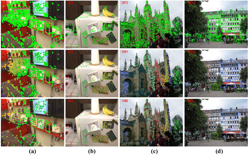
Figure 9: Visualization of sparsification. We remove redundant 3D points according to observations and spatial distributions for each landmark independently. The original 3D points (top), points after filtering with landmarks (middle) and points after sparsification (bottom) on 7Scenes (a), 12Scenes (b), CambridgeLandmarks (c) and Aachen (d) datasets are visualized.

5.3 Map size

Table V shows the map size of APRs [1, 5], SCRs [18, 9], HMs [28, 24, 29, 25], and our system. APRs [1, 3] and SCRs [18, 9] are end-to-end frameworks with 3D map embedded into networks, so we use their model size as the map size for only reference and focus mainly on the comparison between HMs and our approach. We report the number of reference images (#Reference image), 3D points in million (#3D points), 2D descriptor size, global descriptor size, 3D map size, and the total size. Note that for HMs, only local keypoints with 3D correspondences are considered. Obviously, SP+SG [28, 24] has the largest size because of the local and global descriptors. By using smaller dimension (128) of local descriptors than SP [28] (256), SFD2+IMP [29, 25] reduces the size significantly while preserving localization accuracy as shown in Table III, IV and VI.

Although our method also relies on sparse keypoints for recognition and 2D-3D matching, it takes only 10% percent memory size of SFD2+IMP by discarding redundant global features and local features. This is very important to applications on devices with limited computing resources.

5.4 Running time

In this section, we evaluate the average running time of APRs [1, 5, 14, 3], SCRs [9, 18], HMs [28, 24, 21, 29, 25, 21] and our method for processing one image in MarysChurch of CambridgeLandmarks [1] on a machine with RTX3090 GPU and Xeon(R) Silver 4216 CPU@2.10GHz. For fair comparison, we use the same image resolution, number of keypoints, and reconstruction framework [10] for all methods. ResNet34 [90] is adopted as the backbone of APRs and the most recent ACE [9] is adopted as the representative of SCRs.

Table VII shows the time of extracting local [28, 29], global [21] features, recognition, tracking, and pose estimation. APRs [1, 5, 14] runs the fastest as their time cost comes only from feature extraction. SCRs [9] take more time due to time-consuming pose estimation with RANSAC [20] on dense 2D-3D correspondences. SCRs reduce the image resolution and adopt shallower backbones, so they are faster on feature extraction than APRs. For HMs, the time cost comes from the local and global feature extraction and especially the pose estimation. Therefore, HMs are the slowest frameworks.

As HMs, our approach also spends time on local feature extraction. Fortunately, the time of recognition on sparse features is 20ms, 4$\times$ faster than NetVLAD [21]. The tracking component used for verification takes about 310ms due to the graph-based matching. With the initial pose given by tracking, our pose estimation uses only 730ms to recover an accurate pose, which is about 3.5$\times$ and 5.1$\times$ faster than SFD2+IMP+NV and SP+SG+NV, respectively. As a result, the total time of our model is 2.4$\times$ and 3.4$\times$ less than SFD2+IMP+NV and SP+SG+NV. The speed of our model can be further improved by removing the heavy pose estimation component and utilizing the pose provided by tracking as results. By doing that, our model uses 390ms to process each frame and has the cost of only 2% accuracy loss (as shown in Table VIII). Although our approach is faster than HMs and more accurate than APRs and SCRs, there is still a large space for improvements especially on the efficiency.

TABLE VIII: Ablation study. We test the influence of tracking, refinement, sparsification, descriptor dimension and the number of candidate landmarks to pose accuracy.

Sparsification	Tracking	Refinement	Dimension	#Landmarks	Accuracy
✗	✓	✗	128	20	94.5%
✓	✓	✗	128	20	94.3%
✓	✓	✓	128	20	96.8%
✓	✓	✓	64	20	94.9%
✓	✓	✓	32	20	94.3%
✓	✓	✓	0	20	15.8%
✓	✓	✓	128	10	95.3%
✓	✓	✓	128	5	95.1%
✓	✓	✓	128	1	91.7%

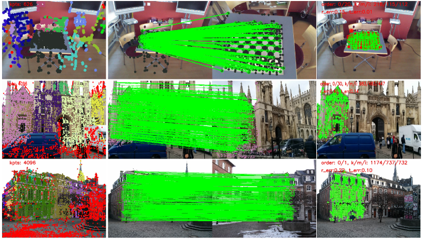
Figure 10: Landmark-wise matching. We visualize predicted landmarks (left), landmark-wise matches (middle), and inliers after registration (right). Results on 7Scenes[37] (row 1), CambridgeLandmarks [1] (row 2), and Aachen [39] (row 3) datasets are included. Predicted landmark labels indicate which keypoints (left, red color) are potential outliers - without 3D points in the Map. Besides, by focusing only points with the same labels, landmark-wise matching is more efficient and accurate.

5.5 Ablation study

We conduct extensive experiments to test the influence of different components in our system including sparsification, tracking, pose refinement (Refinement), dimension of 3D descriptors (Dimension), and the number of candidate landmarks (#Landmarks) for verification. Results on MarysChurch in CambridgeLandmarks at the error threshold of $(25cm,2^{\circ})$ are shown in Table VIII.

From Table VIII, we have the following observations. (1) Sparsification has little influence to the accuracy of our system (94.3% vs. 94.5%) as most discarded 3D points are redundant, whilst stable ones are preserved. (2) Refinement increases the accuracy (96.8% vs. 94.3%) because in the tracking step, only a limited number of 3D points from a single virtual reference frame is used and in the refinement process, more 3D points are further used to refine the pose. (3) When the dimension of 3D descriptors is reduced from 128 to 64 and 32, our model undergoes acceptable loss of accuracy from 96.8% to 94.9% and 94.3%, which means the map size can be further reduced by decreasing the descriptor size. However, when not using 3D descriptors (only 2D coordinates are used), the performance drops significantly from 94.3% to 15.8% compared to using 32-float descriptors because pure locations have very high uncertainties especially for 2D-3D matching. (4) When the number of landmarks used for tracking (#Landmarks) is reduced from 20 to 10, 5 and even 1, our model still gives very robust performance with approximate 5% loss of accuracy (96.8% vs. 91.7%). Note that our model recognizes up to 160 landmarks in the whole CambridgeLandmarks [1]. This observation further enhances the robustness of our sparse recognition strategy.

5.6 Qualitative results

Landmarks. Fig. 8 shows the 3D map and landmarks in 7Scenes [37], 12Scenes [38], CambridgeLandmarks [1], and Aachen [39] datasets. The self-supervised landmark definition allows us to generate landmarks in any places in indoor (pumpkin in 7Scenes, apt1/kitchen in 12Scenes), outdoor (KingsCollege and MarysChurch in CambridgeLandmarks) and even city-scale (Aachen) scenes. This techniques breaks the limitation of classic object classes such as buildings, trees, and so on, as different objects such as ovens and wash machines can be merged as a landmark (apt1/kitchen/12Scenes) and different parts of a building can be divided into different landmarks (MarysChurch/CambdridgeLandmarks).

Sparsification. Fig. 9 shows the sparsified points of images from 7Scenes [37], 12Scenes [38], CambridgeLandmarks [1], and Aachen [39] datasets. The original points are all keypoints with 3D correspondences in the map. Due to insufficient observations, some 3D points have large noise and thus are removed as introduced in Sec. 3.1. Therefore, we can see some points from dynamic objects such as pedestrians (Fig. 9 (c)), tables (Fig. 9 (d)) are filtered. After filtering, there are still a large number of redundant points, so our adaptive pruning strategy discards redundant ones according to their covisibility. After pruning, the number of points for both indoor (Fig. 9 (a)(b)) and outdoor ( 9 (c)(d)) scenes are significantly reduced even up to 50%. Since discard points are those with low stability and remained ones are more robust, the sparsification does not cause obvious performance drop as discussed in Sec. 5.5.

Landmark-wise matching. Fig. 10 shows the landmark-wise matching between query images and the 3D map. The matching is conducted between the query and virtual reference images to reduce the domain differences between 2D and 3D points. Fig. 10 shows the self-defined landmarks provide strong guidance for matching. These landmarks work well in both indoor and outdoor scenes beyond common objects. Fig. 10 (left) also visualizes the potential outliers (red points) which are mainly from dynamics objects and trees. Note that our model is able to discriminate outliers and inliers only according to the matchibility between 2D and 3D points in the training process and no any manually-defined object-level prior is used.

6 Limitations and Open Problems

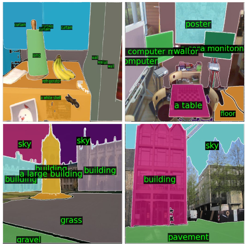
Figure 11: Results of SAM [65] and open-vocabulary recognition. Results of SAM provide object masks which can be used as object-level constraints in the hierarchical clustering process. These objects can be further assigned with semantic labels by open-vocabulary classification models, so that we can build a hierarchical semantic map at the same time.

PRAM is a new framework for visual localization, so many limitations and open problems exist. In this section, we discuss these limitations and open problems and hope following researchers can make PRAM better.

Landmark definition. Our current strategy of generating landmarks considers mainly the spatial connections of points. The object-level consistency is ignored, leading to the split of objects. In the future, we can use SAM [65] results to provide additional object-level connections for 3D points during the hierarchical clustering process, avoiding this problem. Moreover, object labels can also be assigned by open-vocabulary classification models as shown in Fig. 11. In this way, we are able to build a hierarchical map of self-defined and commonly used semantic labels.

In addition to landmark definition, how to decide the number of landmarks is also important. In our experiments, we manually set the number of landmarks for different datasets according to their spatial size, which may not be optimal. An adaptive solution to determining the number of landmarks for a scene is worth of further exploration in the future.

Map sparsification. How to reduce map size including the number of reference images and 3D points remains a challenge in hierarchical frameworks. Previous methods [88, 66, 67] rely mainly on the co-visibility between different reference images. Since images only represent the scene on 2D space rather than the 3D space, resulting in the loss of absolute scale, prior methods usually suffer from over-reduction, impairing the localization accuracy. However, PRAM performs sparsification on the landmarks defined on 3D points with absolute scale of the scene directly, allowing all 3D points to be taken into consideration. Then, by assigning each landmark a virtual reference image, PRAM discards the reference images. Our strategy of conducting sparsification on 3D points first and then reference images may bring insights to map sparsification in HMs.

Map-centric localization. The map contains a lot of useful information but its importance is ignored by previous methods [10, 11, 12, 13, 52] relying purely on reference images. For example, we define the landmarks directly on 3D map as opposed images. Compared to perform semantic segmentation on images, this strategy generalizes well in any scenes and avoids the problem of labeling and dealing with multi-view inconsistency. Besides, the map also tells us which keypoints are inliers and which are not, so that it is not necessary to find a manually-defined metric with low generalization ability for discrimination.

Moreover, PRAM provides a unified framework with only sparse keypoints for recognition and registration. It simplifies previous hierarchical localization framework which requires separate global and local features for coarse and fine localization, independently. Therefore, as opposed to optimizing global and local features separately, PRAM allows us to optimize only local keypoints. In the future, how to extract fewer but more effectively keypoints for localization can be directly optimized with priors of the useful map.

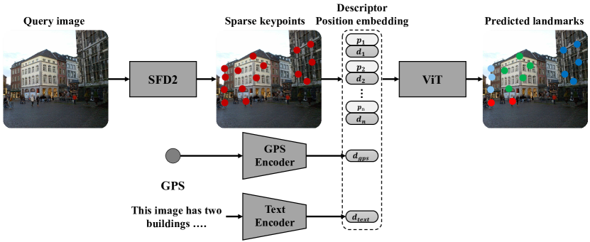
Figure 12: Multi-modality localization. Sparse keypoints extracted from images contain only visual information. In addition to visual information, other signals such as multi-view inputs, GPS, texts can also be used to improve the localization performance as long as they are useful for recognition. The transformer-based recognition module flexibly accepts multi-modality data as input once these signals are encoded as high-level features.

Multi-modality localization. In PRAM framework, recognition is the key to efficient and accurate large-scale localization. As the recognition module takes sparse tokens as input, any other signals such as multi-view images, GPS, electromagnetic signals, texts, voices can be flexibly encoded as tokens to enhance the recognition performance, so as to improve the localization accuracy as shown in Fig. 12.

Let us take GPS as an example. In HMs, the benefit of GPS is squeezing the search space for finding reference images faster and more accurately in outdoor environments. At the same time, HMs have to face problems of inaccurate GPS signals due to the block of high buildings and missing signals in indoor environments, resulting in limited gains of using GPS for anywhere visual localization. However, GPS signals either inaccurate or not, can be used as priors to improve the recognition implicitly. When the GPS is not available in indoor scenes, the GPS token can replaced with a vector of zero values. This can be achieved efficiently and implicitly by recognition module. Such analysis can also be applied to other signals. In a nutshell, for HMs, the gains of using multi-module signals are limited compared to cost, but for PRAM, the gains could be much higher than cost.

Large-scale scene coordinate regression. SCRs cannot report accurate poses in outdoor scenes because of the pixel-wise recognition nature. This problem can be partially solved by the combination with PRAM. Specifically, each landmark in the map built by PRAM is a sub-scene with small scale where SCRs are able to give good results. In the localization process, first, the recognition module gives landmark labels indicating which sub-scene each point belongs to. Then, instead of predicting coordinates in an absolute large scale, SCRs could predict the relative coordinates to small-scale sub-scenes. Finally, the absolute coordinates can be recovered by combining the relative coordinates and sub-scene locations as:

$$X^{r}_{1},...,X^{r}_{n}=f_{SCR}(p_{1},...,p_{n}),$$ (10)

$$L_{1},...,L_{n}=f_{ViT}(p_{1},...,p_{n}),$$ (11)

$$X^{a}_{i}=X^{r}_{i}+\Delta X_{L_{i}}.$$ (12)

$X^{r}_{i}$ and $X^{a}_{i}$ are predicted relative and absolute coordinates for 2D point $p_{i}$. $\Delta X_{L_{i}}$ is the relative coordinate of landmark $L_{i}$ in the map. $f_{SCR}$ is a network for relative coordinate regression. Budvytis et al. [8] try to regress relative coordinates to global instances defined on building facades, but it cannot work in any places as PRAM does. We believe the combination of SCRs and PRAM is worth of exploration in the future.

7 Conclusion

In this paper, we propose a place recognition anywhere model (PRAM) for efficient and accurate localization in all scenes. Specifically, we introduce a map-centric landmark definition strategy to generate self-defined landmarks from bottom to up in an hierarchical manner. This strategy allows us to make any place a landmark, breaking the limitation of commonly used semantic labels. Additionally, PRAM performs visual localization efficiently by recognizing landmarks as opposed to searching reference images in the whole database, which enables our method to discard expensive global and repetitive 2D local descriptors. Moreover, the recognized landmarks are further used for landmark-wise matching instead of exhaustive matching to reduce the time cost. Experiments on indoor 7Scenes, 12Scenes and outdoor CambridgeLandmarks and Aachen datasets demonstrate that PRAM is much faster and memory-efficient than previous hierarchical methods while preserving the accuracy.

As a new localization framework, PRAM has limitations including landmark definition and also opens new directions for localization such as multi-modality recognition, map-centric feature learning and hierarchical scene coordinate regression and so on. We believe that this new framework will benefit the community and hope more researchers to make it better in the future.

References

- [1] A. Kendall, M. Grimes, and R. Cipolla, “Posenet: A convolutional network for real-time 6-dof camera relocalization,” in ICCV, 2015.
- [2] A. Kendall and R. Cipolla, “Geometric loss functions for camera pose regression with deep learning,” in CVPR, 2017.
- [3] F. Xue, X. Wu, S. Cai, and J. Wang, “Learning multi-view camera relocalization with graph neural networks,” in CVPR, 2020.
- [4] S. Brahmbhatt, J. Gu, K. Kim, J. Hays, and J. Kautz, “MapNet: Geometry-aware learning of maps for camera localization,” in CVPR, 2018.
- [5] F. Xue, X. Wang, Z. Yan, Q. Wang, J. Wang, and H. Zha, “Local supports global: Deep camera relocalization with sequence enhancement,” in ICCV, 2019.
- [6] E. Brachmann, A. Krull, S. Nowozin, J. Shotton, F. Michel, S. Gumhold, and C. Rother, “DSAC-differentiable RANSAC for camera localization,” in CVPR, 2017.
- [7] E. Brachmann and C. Rother, “Learning less is more-6d camera localization via 3d surface regression,” in CVPR, 2018.
- [8] I. Budvytis, M. Teichmann, T. Vojir, and R. Cipolla, “Large scale joint semantic re-localisation and scene understanding via globally unique instance coordinate regression,” in BMVC, 2019.
- [9] E. Brachmann, T. Cavallari, and V. A. Prisacariu, “Accelerated coordinate encoding: Learning to relocalize in minutes using rgb and poses,” in CVPR, 2023.
- [10] P.-E. Sarlin, C. Cadena, R. Siegwart, and M. Dymczyk, “From Coarse to Fine: Robust Hierarchical Localization at Large Scale,” in CVPR, 2019.
- [11] F. Xue, I. Budvytis, D. O. Reino, and R. Cipolla, “Efficient Large-scale Localization by Global Instance Recognition,” in CVPR, 2022.
- [12] T. Sattler, B. Leibe, and L. Kobbelt, “Efficient & effective prioritized for large-scale image-based localization,” TPAMI, 2016.
- [13] C. Toft, E. Stenborg, L. Hammarstrand, L. Brynte, M. Pollefeys, T. Sattler, and F. Kahl, “Semantic match consistency for long-term visual localization,” in ECCV, 2018.
- [14] B. Wang, C. Chen, C. X. Lu, P. Zhao, N. Trigoni, and A. Markham, “Atloc: Attention guided camera localization,” in AAAI, 2020.
- [15] X. Wu, H. Zhao, S. Li, Y. Cao, and H. Zha, “Sc-wls: Towards interpretable feed-forward camera re-localization,” in ECCV, 2022.
- [16] J. Shotton, B. Glocker, C. Zach, S. Izadi, A. Criminisi, and A. Fitzgibbon, “Scene coordinate regression forests for camera relocalization in rgb-d images,” in CVPR, 2013.
- [17] X. Li, S. Wang, Y. Zhao, J. Verbeek, and J. Kannala, “Hierarchical scene coordinate classification and regression for visual localization,” in CVPR, 2020.
- [18] E. Brachmann and C. Rother, “Visual camera re-localization from rgb and rgb-d images using dsac,” TPAMI, vol. 44, no. 9, pp. 5847–5865, 2022.
- [19] V. Lepetit, F. Moreno-Noguer, and P. Fua, “Epnp: An accurate o (n) solution to the pnp problem,” IJCV, 2009.
- [20] M. A. Fischler and R. C. Bolles, “Random sample consensus: a paradigm for model fitting with applications to image analysis and automated cartography,” Communications of the ACM, vol. 24, no. 6, pp. 381–395, 1981.
- [21] R. Arandjelovic, P. Gronat, A. Torii, T. Pajdla, and J. Sivic, “NetVLAD: CNN architecture for weakly supervised place recognition,” in CVPR, 2016.
- [22] S. Hausler, S. Garg, M. Xu, M. Milford, and T. Fischer, “Patch-netvlad: Multi-scale fusion of locally-global descriptors for place recognition,” in CVPR, 2021.
- [23] F. Radenović, G. Tolias, and O. Chum, “Fine-tuning cnn image retrieval with no human annotation,” TPAMI, vol. 41, no. 7, pp. 1655–1668, 2018.
- [24] P.-E. Sarlin, D. DeTone, T. Malisiewicz, and A. Rabinovich, “Superglue: Learning feature matching with graph neural networks,” in CVPR, 2020.
- [25] F. Xue, I. Budvytis, and R. Cipolla, “Imp: Iterative matching and pose estimation with adaptive pooling,” in CVPR, 2023.
- [26] H. Chen, Z. Luo, J. Zhang, L. Zhou, X. Bai, Z. Hu, C.-L. Tai, and L. Quan, “Learning to match features with seeded graph matching network,” in ICCV, 2021.
- [27] Y. Shi, J.-X. Cai, Y. Shavit, T.-J. Mu, W. Feng, and K. Zhang, “ClusterGNN: Cluster-based Coarse-to-Fine Graph Neural Network for Efficient Feature Matching,” in CVPR, 2022.
- [28] D. DeTone, T. Malisiewicz, and A. Rabinovich, “Superpoint: Self-supervised interest point detection and description,” in CVPRW, 2018.
- [29] F. Xue, I. Budvytis, and R. Cipolla, “Sfd2: Semantic-guided feature detection and description,” in CVPR, 2023.
- [30] D. G. Lowe, “Distinctive image features from scale-invariant keypoints,” IJCV, 2004.
- [31] E. Rublee, V. Rabaud, K. Konolige, and G. Bradski, “ORB: An efficient alternative to SIFT or SURF,” in ICCV, 2011.
- [32] J. Revaud, P. Weinzaepfel, C. R. de Souza, and M. Humenberger, “R2D2: Repeatable and reliable detector and descriptor,” in NeurIPS, 2019.
- [33] K. M. Yi, E. Trulls, V. Lepetit, and P. Fua, “Lift: Learned invariant feature transform,” in ECCV, 2016.
- [34] F. Langer, G. Bae, I. Budvytis, and R. Cipolla, “Sparc: Sparse render-and-compare for cad model alignment in a single rgb image,” in BMVC, 2022.
- [35] F. Langer, I. Budvytis, and R. Cipolla, “Sparse multi-object render-and-compare,” in BMVC, 2023.
- [36] A. Vaswani, N. Shazeer, N. Parmar, J. Uszkoreit, L. Jones, A. N. Gomez, Ł. Kaiser, and I. Polosukhin, “Attention is all you need,” in NeurIPS, 2017.
- [37] B. Glocker, S. Izadi, J. Shotton, and A. Criminisi, “Real-time rgb-d camera relocalization,” in ISMAR, 2013, pp. 173–179.
- [38] J. Valentin, A. Dai, M. Nießner, P. Kohli, P. Torr, S. Izadi, and C. Keskin, “Learning to navigate the energy landscape,” in 3DV, 2016.
- [39] T. Sattler, T. Weyand, B. Leibe, and L. Kobbelt, “Image retrieval for image-based localization revisited,” in BMVC, 2012.
- [40] X. Li and H. Ling, “Pogo-net: pose graph optimization with graph neural networks,” in ICCV, 2021.
- [41] Li, Xinyi and Ling, Haibin, “Gtcar: Graph transformer for camera re-localization,” in ECCV, 2022.
- [42] M. O. Turkoglu, E. Brachmann, K. Schindler, G. J. Brostow, and A. Monszpart, “Visual camera re-localization using graph neural networks and relative pose supervision,” in 3DV, 2021.
- [43] H. Li, P. Xiong, H. Fan, and J. Sun, “Dfanet: Deep feature aggregation for real-time semantic segmentation,” in CVPR, 2019.
- [44] A. Moreau, N. Piasco, D. Tsishkou, B. Stanciulescu, and A. de La Fortelle, “Lens: Localization enhanced by nerf synthesis,” in CoRL, 2022.
- [45] T. Sattler, Q. Zhou, M. Pollefeys, and L. Leal-Taixe, “Understanding the limitations of cnn-based absolute camera pose regression,” in CVPR, 2019.
- [46] N.-D. Duong, A. Kacete, C. Soladie, P.-Y. Richard, and J. Royan, “Accurate sparse feature regression forest learning for real-time camera relocalization,” in 3DV, 2018.
- [47] J. Sivic and A. Zisserman, “Efficient visual search of videos cast as text retrieval,” TPAMI, vol. 31, no. 4, pp. 591–606, 2008.
- [48] D. Gálvez-López and J. D. Tardos, “Bags of binary words for fast place recognition in image sequences,” T-RO, vol. 28, no. 5, pp. 1188–1197, 2012.
- [49] E. Stenborg, C. Toft, and L. Hammarstrand, “Long-term visual localization using semantically segmented images,” in ICRA, 2018.
- [50] T. Shi, S. Shen, X. Gao, and L. Zhu, “Visual localization using sparse semantic 3D map,” in ICIP, 2019.
- [51] Z. Xin, Y. Cai, T. Lu, X. Xing, S. Cai, J. Zhang, Y. Yang, and Y. Wang, “Localizing discriminative visual landmarks for place recognition,” in ICRA, 2019.
- [52] M. Larsson, E. Stenborg, C. Toft, L. Hammarstrand, T. Sattler, and F. Kahl, “Fine-grained segmentation networks: Self-supervised segmentation for improved long-term visual localization,” in ICCV, 2019.
- [53] R. F. Salas-Moreno, R. A. Newcombe, H. Strasdat, P. H. Kelly, and A. J. Davison, “Slam++: Simultaneous localisation and mapping at the level of objects,” in CVPR, 2013.
- [54] V. Badrinarayanan, A. Kendall, and R. Cipolla, “Segnet: A deep convolutional encoder-decoder architecture for image segmentation,” TPAMI, 2017.
- [55] L.-C. Chen, Y. Zhu, G. Papandreou, F. Schroff, and H. Adam, “Encoder-decoder with atrous separable convolution for semantic image segmentation,” in ECCV, 2018.
- [56] R. Mur-Artal and J. D. Tardós, “ORB-SLAM2: an open-source SLAM system for monocular, stereo and RGB-D cameras,” IEEE TRO, vol. 33, no. 5, pp. 1255–1262, 2017.
- [57] F. Xue, X. Wang, S. Li, Q. Wang, J. Wang, and H. Zha, “Beyond tracking: Selecting memory and refining poses for deep visual odometry,” in CVPR, 2019.
- [58] S. Li, F. Xue, X. Wang, Z. Yan, and H. Zha, “Sequential adversarial learning for self-supervised deep visual odometry,” in ICCV, 2019.
- [59] I. Budvytis, P. Sauer, and R. Cipolla, “Semantic localisation via globally unique instance segmentation,” in BMVC, 2018.
- [60] J. L. Schönberger and J.-M. Frahm, “Structure-from-motion revisited,” in CVPR, 2016.
- [61] M. Dusmanu, I. Rocco, T. Pajdla, M. Pollefeys, J. Sivic, A. Torii, and T. Sattler, “D2-Net: A trainable CNN for joint description and detection of local features,” in CVPR, 2019.
- [62] M. J. Tyszkiewicz, P. Fua, and E. Trulls, “DISK: Learning local features with policy gradient,” in NeurIPS, 2020.
- [63] T. Zhang, R. Ramakrishnan, and M. Livny, “BIRCH: an efficient data clustering method for very large databases,” ACM sigmod record, vol. 25, no. 2, pp. 103–114, 1996.
- [64] D. Arthur and S. Vassilvitskii, “K-means++ the advantages of careful seeding,” in Proceedings of the eighteenth annual ACM-SIAM symposium on Discrete algorithms, 2007.
- [65] A. Kirillov, E. Mintun, N. Ravi, H. Mao, C. Rolland, L. Gustafson, T. Xiao, S. Whitehead, A. C. Berg, W.-Y. Lo, P. Dollár, and R. Girshick, “Segment anything,” in ICCV, 2023.
- [66] Y. Li, N. Snavely, and D. P. Huttenlocher, “Location recognition using prioritized feature matching,” in ECCV, 2010.
- [67] H. Soo Park, Y. Wang, E. Nurvitadhi, J. C. Hoe, Y. Sheikh, and M. Chen, “3d point cloud reduction using mixed-integer quadratic programming,” in CVPRW, 2013.
- [68] J. L. Schönberger, M. Pollefeys, A. Geiger, and T. Sattler, “Semantic visual localization,” in CVPR, 2018.
- [69] Y. Shavit and Y. Keller, “Camera pose auto-encoders for improving pose regression,” in ECCV, 2022.
- [70] Y. Shavit, R. Ferens, and Y. Keller, “Learning multi-scene absolute pose regression with transformers,” in ICCV, 2021.
- [71] Z. Huang, H. Zhou, Y. Li, B. Yang, Y. Xu, X. Zhou, H. Bao, G. Zhang, and H. Li, “VS-Net: Voting with segmentation for visual localization,” in CVPR, 2021.
- [72] P.-E. Sarlin, A. Unagar, M. Larsson, H. Germain, C. Toft, V. Larsson, M. Pollefeys, V. Lepetit, L. Hammarstrand, F. Kahl et al., “Back to the feature: learning robust camera localization from pixels to pose,” in CVPR, 2021.
- [73] M. Ding, Z. Wang, J. Sun, J. Shi, and P. Luo, “Camnet: Coarse-to-fine retrieval for camera re-localization,” in ICCV, 2019.
- [74] L. Yang, Z. Bai, C. Tang, H. Li, Y. Furukawa, and P. Tan, “Sanet: Scene agnostic network for camera localization,” in ICCV, 2019.
- [75] L. Zhou, Z. Luo, T. Shen, J. Zhang, M. Zhen, Y. Yao, T. Fang, and L. Quan, “Kfnet: Learning temporal camera relocalization using kalman filtering,” in Proceedings of the IEEE/CVF conference on computer vision and pattern recognition, 2020.
- [76] J. Liu, Q. Nie, Y. Liu, and C. Wang, “Nerf-loc: Visual localization with conditional neural radiance field,” in ICRA, 2023.
- [77] S. Tang, C. Tang, R. Huang, S. Zhu, and P. Tan, “Learning camera localization via dense scene matching,” in CVPR, 2021.
- [78] A. Paszke, S. Gross, F. Massa, A. Lerer, J. Bradbury, G. Chanan, T. Killeen, Z. Lin, N. Gimelshein, L. Antiga et al., “Pytorch: An imperative style, high-performance deep learning library,” in NeurIPS, 2019.
- [79] D. P. Kingma and J. Ba, “Adam: A method for stochastic optimization,” in ICLR, 2015.
- [80] I. Rocco, R. Arandjelović, and J. Sivic, “Efficient neighbourhood consensus networks via submanifold sparse convolutions,” in ECCV, 2020.
- [81] Z. Huang, H. Zhou, Y. Li, B. Yang, Y. Xu, X. Zhou, H. Bao, G. Zhang, and H. Li, “Vs-net: Voting with segmentation for visual localization,” in Proceedings of the IEEE/CVF Conference on Computer Vision and Pattern Recognition, 2021.
- [82] L. Svärm, O. Enqvist, F. Kahl, and M. Oskarsson, “City-scale localization for cameras with known vertical direction,” TPAMI, 2016.
- [83] W. Cheng, W. Lin, K. Chen, and X. Zhang, “Cascaded parallel filtering for memory-efficient image-based localization,” in ICCV, 2019.
- [84] T. Sattler, W. Maddern, C. Toft, A. Torii, L. Hammarstrand, E. Stenborg, D. Safari, M. Okutomi, M. Pollefeys, J. Sivic et al., “Benchmarking 6dof outdoor visual localization in changing conditions,” in CVPR, 2018.
- [85] E. Brachmann and C. Rother, “Expert sample consensus applied to camera re-localization,” in CVPR, 2019.
- [86] S. Tang, S. Tang, A. Tagliasacchi, P. Tan, and Y. Furukawa, “Neumap: Neural coordinate mapping by auto-transdecoder for camera localization,” in CVPR, 2023, pp. 929–939.
- [87] W. Cheng, W. Lin, K. Chen, and X. Zhang, “Cascaded parallel filtering for memory-efficient image-based localization,” in ICCV, 2019.
- [88] L. Yang, R. Shrestha, W. Li, S. Liu, G. Zhang, Z. Cui, and P. Tan, “Scenesqueezer: Learning to compress scene for camera relocalization,” in CVPR, 2022.
- [89] Z. Luo, L. Zhou, X. Bai, H. Chen, J. Zhang, Y. Yao, S. Li, T. Fang, and L. Quan, “ASLFeat: Learning local features of accurate shape and localization,” in CVPR, 2020.
- [90] K. He, X. Zhang, S. Ren, and J. Sun, “Deep residual learning for image recognition,” in CVPR, 2016.