ConsistencyDet: A Robust Object Detector with a Denoising Paradigm of Consistency Model

Abstract

Object detection, a quintessential task in the realm of perceptual computing, can be tackled using a generative methodology. In the present study, we introduce a novel framework designed to articulate object detection as a denoising diffusion process, which operates on the perturbed bounding boxes of annotated entities. This framework, termed ConsistencyDet, leverages an innovative denoising concept known as the Consistency Model. The hallmark of this model is its self-consistency feature, which empowers the model to map distorted information from any temporal stage back to its pristine state, thereby realizing a “one-step denoising” mechanism. Such an attribute markedly elevates the operational efficiency of the model, setting it apart from the conventional Diffusion Model. Throughout the training phase, ConsistencyDet initiates the diffusion sequence with noise-infused boxes derived from the ground-truth annotations and conditions the model to perform the denoising task. Subsequently, in the inference stage, the model employs a denoising sampling strategy that commences with bounding boxes randomly sampled from a normal distribution. Through iterative refinement, the model transforms an assortment of arbitrarily generated boxes into definitive detections. Comprehensive evaluations employing standard benchmarks, such as MS-COCO and LVIS, corroborate that ConsistencyDet surpasses other leading-edge detectors in performance metrics. Our code is available at https://github.com/Tankowa/ConsistencyDet.

1 Introduction

Object detection, a cornerstone task in the realm of computer vision, involves predicting both positional data and categorical identities for objects within each image [1, 2, 3]. It serves as the foundation for a wide array of applications, encompassing instance segmentation, pose estimation, action recognition, object tracking, and the detection of visual relationships[4, 5, 6, 7, 8]. Initial object detection methods centered on strategies employing sliding windows and region proposals to delineate object candidate regions, utilizing surrogate techniques for regression and classification [9, 10]. While these methods demonstrated some level of effectiveness, they were impeded by the manual design of candidate selection processes, which hampered their adaptability in complex visual contexts. The introduction of anchor boxes offered increased flexibility, enabling models to better accommodate objects of diverse scales and aspect ratios through pre-established anchor points [11, 12]. Despite this improvement, reliance on a priori information persisted, limiting the universality of these methods across various datasets and scenes. In recent years, the field of object detection has shifted from reliance on empirical object priors to the utilization of learnable object queries or proposals [13, 14]. A seminal development in this direction is the Detection Transformer (DETR), which marked a paradigm shift by employing learnable object queries, thereby recasting object detection as an end-to-end learning challenge [13]. This innovative strategy eradicated the need for hand-crafted components, garnering significant interest in the research community. Concurrently, the Transformer architecture offered novel perspectives, registering impressive achievements across a spectrum of visual recognition tasks. This movement fostered the emergence of query-based detection models [15, 16], introducing a wave of ingenuity and breadth to the field of object detection. Notably, Transformer models have excelled beyond conventional CNN-based detectors, particularly distinguishing themselves in the domain of small object detection (SOD) techniques.

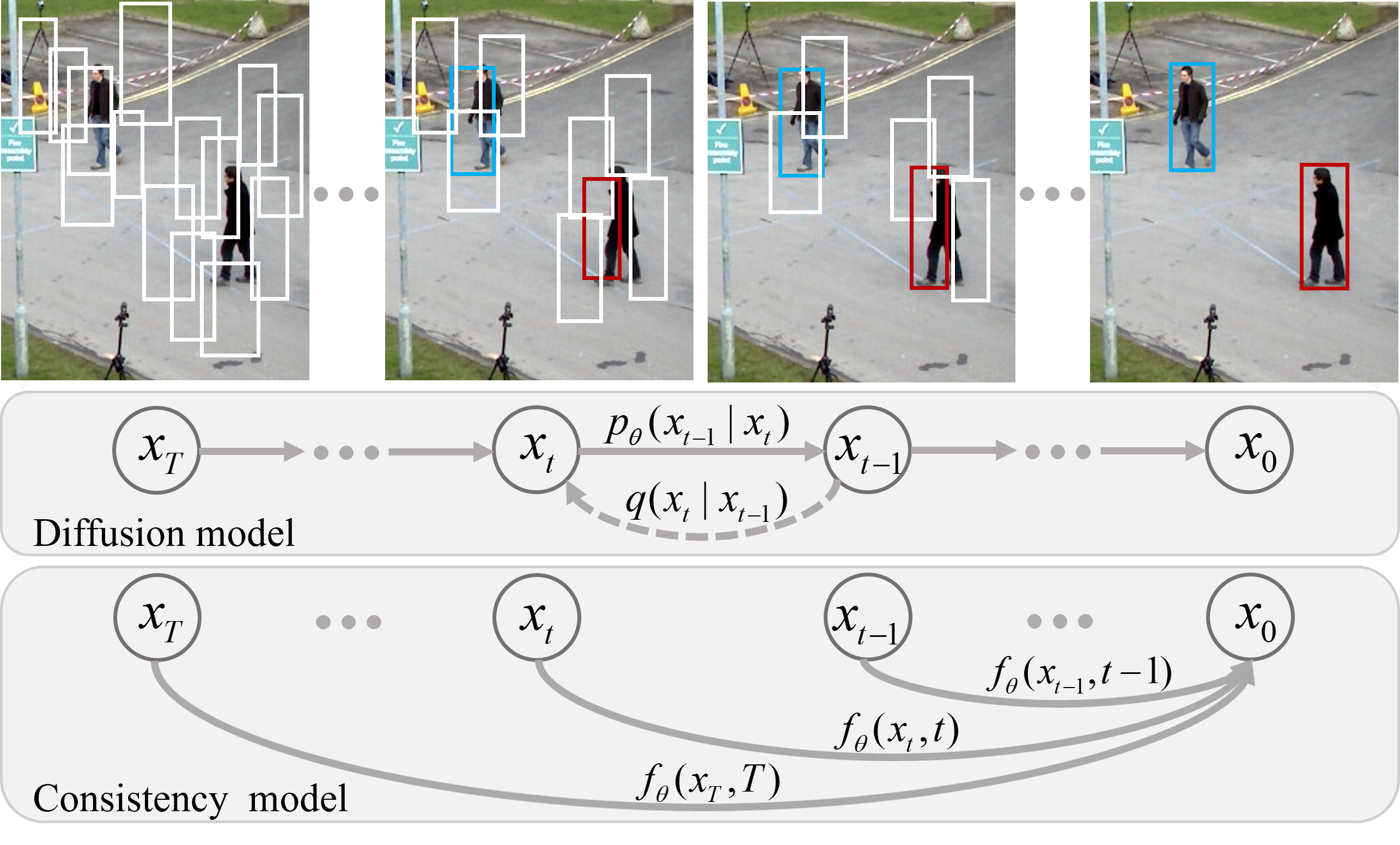
Figure 1: Comparisons of denoising strategies of the Diffusion Model and Consistency Model for object detection. Object detection can be regarded as a denoising diffusion process from noisy boxes to object boxes. In the Diffusion Model, $q(\cdot|\cdot)$ is the diffusion process and $p_{\theta}(\cdot|\cdot)$ is the reverse process with a stepwise denoising operation. In the Consistency Model, $f_{\theta}(\cdot,\cdot)$ represents a one-step denoising process.

Recently, the Diffusion Model [17, 18], also known as a score-based generative model, has demonstrated remarkable effectiveness in a variety of domains, including image generation [19], image segmentation [20], and object detection [21]. A defining characteristic of the Diffusion Model is its iterative sampling mechanism, which methodically reduces noise from an initially random vector. This approach can be adeptly applied to object detection by starting with a set of stochastic bounding boxes. The process begins with entirely random boxes, free from learnable parameters that require training optimization. Through iterative refinement, the method aims to incrementally improve the accuracy of the bounding boxes’ positions and scales. The ultimate goal is to achieve exhaustive delineation of objects within focused categories. This ”noise-to-box” methodology eliminates the need for heuristic object priors or trainable queries, thereby simplifying the selection of object candidates and fostering progress in the development of object detection.

Building on the principles of the Diffusion Model, DiffusionDet has outperformed various existing detectors, even surpassing the paradigm established by the Transformer model [21]. Yet, its stepwise denoising process, mirroring the iterations of noise addition, imposes constraints on both flexibility and computational efficiency. To render the model viable for real-world applications, these constant iterations require further optimization. Addressing this issue, we propose an innovative approach with the Consistency Model [22], herein referred to as ConsistencyDet. Our model is deeply informed by the foundational concepts of DiffusionDet. A comparative analysis of the denoising strategies employed by the Consistency Model and the Diffusion Model is illustrated in Fig. 1. Distinctly, the self-consistency property of the Consistency Model enables a one-step denoising process, significantly enhancing execution efficiency. Consequently, the number of denoising iterations can be dramatically reduced while maintaining the integrity of detection accuracy.

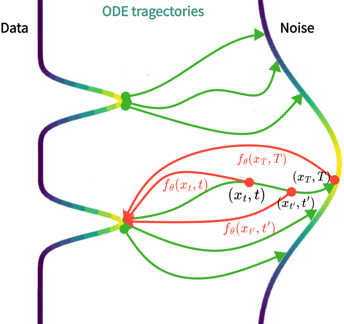
Figure 2: Consistency Model undergoes training process to establish a mapping that brings points along any trajectory of the PF ODE back to the origin of that trajectory [22].

As depicted in Fig. 2, our method builds upon the ordinary differential equation (ODE) framework for probability flow (PF) as utilized in the continuous-time model of DiffusionDet [23]. These models effectively direct sample paths, enabling a smooth transition from the initial data distribution to a tractable noise distribution. ConsistencyDet is distinctive in that it maps any given point from an arbitrary time step back to the origin of its trajectory. Thanks to the self-consistency feature of the model, points along the same trajectory correspond to the same initial point. This innovative approach allows for the generation of data samples, originated by the initial points of ODE trajectories, by transforming random noise vectors through a single evaluation of the network. It is worth noting, however, that the Box-renewal operation, which is conducted by amalgamating new proposals with the remaining outputs from ConsistencyDet across various time steps, does improve sample quality, but this comes at an additional computational expense. Nevertheless, the proposed ConsistencyDet achieves cost-effective iterative sampling, akin to the process employed by DiffusionDet.

The proposed ConsistencyDet model innovatively incorporates Gaussian noise [24] into the center coordinates and sizes of the actual bounding boxes within images, thereby generating noisy boxes. These noisy boxes are then employed to extract features from the regions of interest (RoI) [10], which are delineated on the comprehensive output feature maps produced by the backbone encoder, including ResNet-50 [25], ResNet-101 [25], and Swin Transformer [26]. Subsequently, the RoI features are inputted into the detection decoder, which aims to accurately predict the ground truth (GT) boxes devoid of noise. As a result, ConsistencyDet demonstrates the capability to infer actual bounding boxes from randomized boxes, effectively fulfilling the object detection task. During the inference phase, ConsistencyDet generates bounding boxes by inversely applying the learned diffusion process.

Moreover, the performance of the proposed ConsistencyDet model has been rigorously assessed on the challenging datasets of MS-COCO and LVIS v1.0 [27, 28]. Supported by a variety of backbone architectures, including ResNet-50 [25], ResNet-101 [25], and Swin-Base [26], ConsistencyDet exhibits commendable performance. Our work contributes to the field in the following ways:

• We conceptualize object detection as a generative denoising process and propose a novel methodological approach. In contrast to the established paradigm in DiffusionDet, which employs an equal number of iterations for noise addition and removal, our method represents a substantial advancement in enhancing the efficiency of the detection task.

• In the proposed ConsistencyDet, we engineered a noise addition and removal paradigm that does not impose specific architectural constraints, thereby allowing for flexible parameterization with a variety of neural network structures. This design choice significantly augments the model’s practicality and adaptability for diverse applications.

• In crafting the loss function for the proposed ConsistencyDet, we aggregate the individual loss values at time steps $t$ and $t-1$ subsequent to the model’s predictions to compute the total loss. This methodology guarantees that the mapping of any pair of adjacent points along the temporal dimension to the axis origin maintains the highest degree of consistency. This attribute mirrors the inherent self-consistency principle central to the Consistency Model.

The remainder of this paper is structured as follows: Section 2 offers a concise review of the evolution of object detection models, examines the extensive applications of Diffusion Models, and discusses the foundational principles of the Consistency Model. Subsequently, Section 3 delineates the specific methodologies employed for noise addition and removal within the Consistency Model, elucidates the model’s architecture, and provides essential details pertaining to training and sampling methodologies. Section 4 details the empirical findings obtained from evaluating ConsistencyDet and conducts a comparative analysis against other leading models in the field. The paper concludes with Section 5, which encapsulates the salient features of the newly proposed ConsistencyDet and contemplates avenues for prospective research.

2 Related works and nomenclature

2.1 Object detection

Object detection has undergone significant evolution across various phases. In the initial stages, researchers employed traditional image processing techniques, endeavoring to detect objects by employing methods such as edge detection and feature extraction. These methods, however, encountered considerable challenges when dealing with complex scenes and variations in illumination. With the advent of deep learning, seminal frameworks such as R-CNN and Fast R-CNN [9] have enhanced detection capabilities in terms of speed and accuracy. This was achieved through the integration of innovative concepts like Region Proposal Networks and RoI Pooling. Subsequent developments led to the emergence of single-stage detectors, including YOLO and SSD, which offered improvements in real-time performance, facilitating rapid end-to-end object detection. More recently, the introduction of attention-based Transformer methods, exemplified by DETR [13], has propelled object detection to unprecedented levels of performance, enabling more precise object localization by leveraging global visual context modeling. Although these detection methods have demonstrated noteworthy effectiveness, there remains considerable potential for further advancement. In the present work, we introduce an innovative detection approach that iteratively refines the position and size of bounding boxes. This refinement process employs a series of noisy iterations, culminating in the bounding boxes precisely encompassing the target object.

2.2 Diffusion Model for perception tasks

The Diffusion Model [24, 23], a subset of deep generative models, has emerged as a powerful tool that originates from random distribution samples and gradually reconstructs the expected data through a denoising process. This model has recently achieved remarkable success in a range of fields, including computer vision [18], natural language processing [29], audio signal processing [30], and interdisciplinary applications [31], as highlighted in recent surveys [32]. In the context of object detection, the Diffusion Model has been adapted into a detector termed DiffusionDet [21], which reframes the object detection challenge as a set prediction problem. This involves the assignment of object candidates to GT boxes. DiffusionDet represents a groundbreaking application of the Diffusion Model to the field of object detection. Building upon the foundations of DiffusionDet, our work seeks to optimize the balance between detection accuracy and computational speed. We aim to enhance detection efficiency through a single-step processing approach, while preserving the essential benefits derived from iterative sampling

Notation	Definition
$T$	Number of total time steps
$t$	Current time step
$t_{r}$	A random time step in the range $[0,T]$
$\Delta t$	Time step interval for sampling
$\textit{c}_{x}^{\textit{i}}/\textit{c}_{y}^{\textit{i}}$	$x/y$-axis coordinate of the $i$-th box’s center point
$\textit{w}^{\textit{i}}/\textit{h}^{\textit{i}}$	Width ​/​ Height of the $i$-th box
$\textit{b}^{\textit{i}}$	$(\textit{c}_{x}^{\textit{i}},\textit{c}_{y}^{\textit{i}},\textit{w}^{\textit{i}},\textit{h}^{\textit{i}})$ of the $i$-th box
$\alpha_{t}/\sigma_{t}$	Parameter in Denoiser at the $t$-th time step
$\theta$	Model parameter
$F_{\theta}(\cdot,\cdot)$	A designed free-form deep neural network
$\mathcal{N}(\cdot,\cdot)$	Normal distribution
$f_{\theta}(\cdot,\cdot)$	Final answer for Consistency Model
$c_{skip/out/in}(\cdot)$	Calculation factor for $f_{\theta}$
$d(\cdot,\cdot)$	Distance function
$\eta$	Learning rate
$\mu$	EMA decay rate
$\Phi(\cdot,\cdot;\phi)$	ODE solver
$\lambda(\cdot)$	A positive weighting function
$\mathcal{L}$	Total loss function in training process
$\mathcal{L}_{cls/L1/giou}$	Focal ​/​ L1 ​/​ GIoU loss item
$\lambda_{cls/L1/giou}$	Weight for Focal ​/​ L1 ​/​ GIoU loss item
$\sigma_{max/min}$	Maximum ​/​ Minimum threshold of noise parameter
$\sigma_{data}$	Noise parameter between $\sigma_{min}$ and $\sigma_{max}$
$\epsilon$	Randomly generated Gaussian noise
$\rho$	Scale factor of generated noise
$B_{t}$	Random noise at the $t$-th time step in sampling
$r(\cdot)$	Generate random noise with given dimensions
$E(\cdot)$	Image feature extraction with backbone network
$P_{c}(\cdot,\cdot)$	Prediction of Consistency Model in each time step
$nms(\cdot,\cdot)$	Non-max suppression (NMS) operation
Nth	Threshold of NMS operation
Bth	Threshold of Box-renewal operation
$dcm(\cdot,\cdot)$	Decoder of ConsistencyDet with head network
$ddm(\cdot,\cdot)$	Denoiser of DiffusionDet with head network
$conc(\cdot,\cdot)\$	Concatenate function
$n_{ss}$	Number of sampling steps
$n_{p}$	Number of total proposed boxes
$n_{r}$	Number of current proposed boxes
$x_{s}$	Padded box information at time axis origin
$x_{t}$	Noised box information at the $t$-th time step
$x_{b}$	Predicted box information in each time step
$x_{0}$	Predicted box information at time axis origin
$x_{box/cls}$	Predicted object’s box coordinate ​/​ category
AP	Average Precision
AP50/75	Average Precision at 50% ​/​ 75% IoU
APs/m/l	Average Precision for small ​/​ median ​/​ large objects
APr/c/f	Average​ Precision​ for​ rare ​/​ common ​/​ frequent​ categories

TABLE I: Nomenclature with related notations.

2.3 Consistency Model

The Diffusion Model is predicated on an iterative generation process, which tends to result in sluggish execution efficiency, thus curtailing its applicability in real-time scenarios. To address this limitation, OpenAI has unveiled the Consistency Model, an innovative category of generative models capable of rapidly producing high-quality samples without necessitating adversarial training regimes. The Consistency Model facilitates swift one-step generation, yet it retains the option for multi-step sampling as a means to navigate the trade-off between computational efficiency and the caliber of generated samples. Furthermore, it introduces the capability for zero-shot [33] data manipulation, encompassing tasks such as image restoration, colorization, and super-resolution, obviating the need for task-specific training.

The Consistency Model can be cultivated through a distillation pre-training regimen derived from existing Diffusion Models or alternatively as a standalone generative model. This work formally acknowledges this capability and, for the inaugural time, incorporates the Consistency Model within the domain of object detection, hereby designated as ConsistencyDet.

2.4 Nomenclature

For the sake of clarity in the ensuing discussion, we provide a summary of the symbols and their corresponding descriptions as utilized in this study. This is encapsulated in Table I, which meticulously outlines the nomenclature employed. The symbols encompass a variety of elements including training samples, components of the loss function, strategies for training, and metrics for evaluation, among others.

3 Proposed detection method

3.1 Preliminaries

Object Information. In the domain of object detection, datasets consist of input-target pairs denoted as ($\mathit{x}$, $\mathit{b}$, $\mathit{c}$), where $\mathit{x}$ represents an input image, $\mathit{b}$ denotes the set of bounding boxes for objects within the image, and $\mathit{c}$ signifies the corresponding set of category labels for those objects. More precisely, the $i$-th bounding box in the set $\mathit{b}$ can be quantified as $\mathit{b}^{i}=(\mathit{c}_{x}^{i},\mathit{c}_{y}^{i},\mathit{w}^{i},\mathit{h}^{i})$, where the coordinates $(\mathit{c}_{x}^{i},\mathit{c}_{y}^{i})$ specify the center of the bounding box along the x-axis and y-axis, respectively, while the terms $(\mathit{w}^{i},\mathit{h}^{i})$ define the width and height of the bounding box.

Diffusion Model. Diffusion Models can be principally categorized into two types: Denoising Diffusion Probabilistic Models (DDPM) [24] and Denoising Diffusion Implicit Models (DDIM) [34]. DDIM is an optimized variant of DDPM, where the generation process is modified. For DDIM, the procedure commences by predicting $x_{0}$ from $x_{t}$ and subsequently inferring $x_{t-1}$ from $x_{0}$. Here, $x_{0}$ acts as an anchor point, enabling the generation process to navigate through arbitrary time steps, thus circumventing the temporal constraints intrinsic to DDPM. While the diffusion process and the training methodology of DDIM parallels that of DDPM, the sampling process in DDIM ceases to be a Markov chain because $x_{t-1}$ is contingent not only on $x_{t}$ but also on $x_{0}$.

At any given moment, $x_{0}$ can be derived from $x_{t}$ and $\epsilon$ iteratively, using the following relationship:

$$f_{\theta}^{(t)}(x_{t})=\frac{x_{t}-\sqrt{1-\alpha_{t}}\cdot\epsilon_{\theta}^{(t)}(x_{t})}{\sqrt{\alpha_{t}}}.$$ (1)

Subsequently, $x_{t-1}$ is predicted based on the neural network’s output as per the equation:

$$p_{\theta}^{(t)}(x_{t-1}|x_{t})=\begin{cases}\mathcal{N}(f_{\theta}^{(1)}(x_{1}),\sigma_{1}^{2}\mathbf{I})&\text{if }t=1,\\ q_{\sigma}(x_{t-1}|x_{t},f_{\theta}^{(t)}(x_{t}))&\text{otherwise}.\end{cases}$$ (2)

When $x_{0}$ and $x_{t-1}$ (for $t>1$) are given, the forward process is rendered deterministic. The generation of latent variable samples employs a consistent strategy, designated as the DDIM. The fundamental principle of DDIM is encapsulated in the equation:

$$\begin{split}x_{t-1}=&\sqrt{\alpha_{t-1}}\left(\frac{x_{t}-\sqrt{1-\alpha_{t}}\cdot\epsilon_{\theta}^{(t)}(x_{t})}{\sqrt{\alpha_{t}}}\right)\\ &+\sqrt{1-\alpha_{t-1}-\sigma_{t}^{2}}\cdot\epsilon_{\theta}(x_{t},t)+\sigma_{t}\epsilon_{t}.\end{split}$$ (3)

In this formulation, DDIM presents a refined approach to generating samples, affording a significant enhancement in efficiency over the traditional DDPM framework.

Consistency Model. In this study, within the framework of the Consistency Model which utilizes deep neural networks, we investigate two cost-effective methodologies for enforcing boundary conditions. Let $F_{\theta}(x,t)$ represent a free-form deep neural network whose dimensionality is the same as $x$. The first method directly parameterizes the Consistency Model as:

$$f_{\theta}(x,t)=\begin{cases}x&\text{if }t=\tau,\\ F_{\theta}(x,t)&\text{if }t\in[\tau,T),\end{cases}$$ (4)

where $\tau$ is an integer in the range $[0,T-1]$. The second method parameterizes the Consistency Model by incorporating skip connections and is formalized as follows:

$$f_{\theta}(x,t)=c_{\text{skip}}(t)x+c_{\text{out}}(t)F_{\theta}(x,t),$$ (5)

where $c_{\text{skip}}(t)$ and $c_{\text{out}}(t)$ are differentiable functions [22], satisfying $c_{\text{skip}}(\tau)=1$ and $c_{\text{out}}(\tau)=0$. By employing this construction, the Consistency Model becomes differentiable at $t=\tau$, provided that $F_{\theta}(x,t)$, $c_{\text{skip}}(t)$, and $c_{\text{out}}(t)$ are all differentiable. This differentiability is crucial for the training of continuous-time Consistency Models.

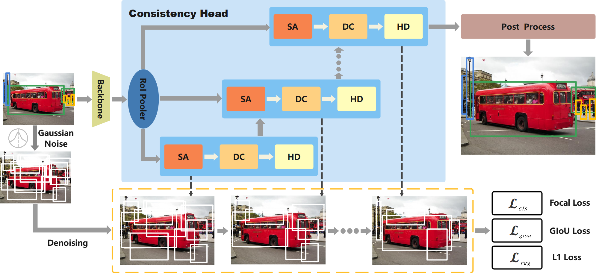
Figure 3: Training procedures of the proposed ConsistencyDet. After extracting features through the backbone, random Gaussian noise is added to GT boxes following the Consistency Model’s noise addition strategy. These noised boxes with corresponding features processed by RoI pooler are then input to ConsistencyHead for iterative noise removal, with several basic modules, ultimately yielding the final detection results. Each the basic module contains a self-attention mechanism (SA), dynamic convolutional layers (DC) and the head (HD) of classification and regression.

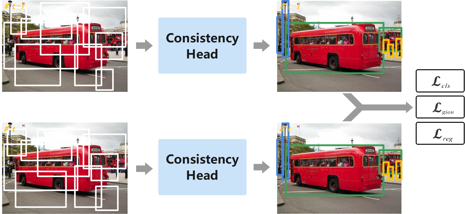
Figure 4: To ensure the self-consistency property of the Consistency Model, it requires feeding the noised boxes corresponding to $(t-1)$-th and $t$-th time steps into the model simultaneously. They jointly predict the final results, then compare them with GT to estimate the training loss.

Training process of Consistency Model. Within the context of the Consistency Model, this study introduces two different training strategies that capitalize on the self-consistency property. The proposed strategies encompass distillation training, which transfers knowledge from a Diffusion Model to the Consistency Model, and an autonomous training regime where the Consistency Model is trained independently.

The first method employs numerical ODE solvers in conjunction with a pre-trained diffusion-based detector, referred to as DiffusionDet, to generate pairs of proximate points along a PF ODE trajectory. By minimizing the divergence between the model predictions for these point pairs, knowledge from the Diffusion Model is effectively transferred to the Consistency Model. As a result, this allows for the generation of high-quality samples through a single evaluation of the network [35, 36]. The comprehensive training protocol for the Consistency Model through distillation is encapsulated in Algorithm 1.

Conversely, the second approach dispenses with the need for a pre-trained Diffusion Model, thereby enabling the Consistency Model to be trained in a standalone manner. This technique delineates the Consistency Model as an independent entity within the broader spectrum of its applications. The detailed training process for the independently trained Consistency Model is encapsulated in Algorithm 2.

Input: Dataset $\mathcal{D}$, initial model parameter $\theta$, learning rate $\eta$, ODE solver $\Phi(\cdot,\cdot;\phi)$, distance function $d(\cdot,\cdot)$, temperature function $\lambda(\cdot)$, and $\mu$

Output: Final trained model parameter $\theta$

1

2$\theta^{-}\leftarrow\theta$

3while not convergence do

4       Sample $x\in\mathcal{D}$ and $n\in U[1,N-1]$;

5       Sample $x_{\sigma_{t+1}}\in\mathcal{N}(x,\sigma_{t+1}^{2}I)$;

6       $\bar{x}_{\sigma_{t}}^{\phi}\leftarrow x_{\sigma_{t+1}}+(\sigma_{t}-\sigma_{t+1})\Phi(x_{\sigma_{t+1}},\sigma_{t+1};\phi)$;

7       $\mathcal{L}(\theta,\theta^{-};\phi)\leftarrow\lambda({\sigma_{t}})d(f_{\theta}(x_{\sigma_{t+1}},\sigma_{t+1}),f_{\theta^{-}}(\bar{x}_{\sigma_{t}}^{\phi},\sigma_{t}))$;

8       $\theta\leftarrow\theta-\eta\nabla_{\theta}\mathcal{L}(\theta,\theta^{-};\phi)$;

9       $\theta^{-}\leftarrow\text{stopgrad}(\mu\theta^{-}+(1-\mu)\theta)$;

10      

11 end while

return $\theta$

Algorithm 1 Consistency Distillation (CD)

Input: Dataset $\mathcal{D}$, initial model parameter $\theta$, learning rate $\eta$, step schedule $T(\cdot)$, EMA decay rate schedule $\mu(\cdot)$, $d(\cdot,\cdot)$, and $\lambda(\cdot)$

1

Output: Updated model parameter $\theta$

2

3$\theta^{-}\leftarrow\theta$ and $k\leftarrow 0$

4while not convergence do

5       Sample $\mathbf{x}\in\mathcal{D}$, and $t\in\mathcal{U}\left[1,T(k)-1\right]$;

6      Sample $\epsilon\in\mathcal{N}(0,I)$;

7      $\mathcal{L}(\theta,\theta^{-})\leftarrow\lambda(\sigma_{t})d(f_{\theta}\left(\mathbf{x}+\epsilon\sigma_{t+1},\sigma_{t+1}\right),f_{\theta^{-}}\left(\mathbf{x}+\epsilon\sigma_{t},\sigma_{t}\right))$;

8      $\theta\leftarrow\theta-\eta\nabla_{\theta}\mathcal{L}(\theta,\theta^{-})$;

9      $\theta^{-}\leftarrow\text{stopgrad}(\mu(k)\theta^{-}+(1-\mu(k))\theta)$;

10      $k\leftarrow k+1$;

11 end while

return $\theta$

Algorithm 2 Consistency Training (CT)

3.2 Architecture

ConsistencyDet is composed of an image encoder and a detection decoder, with the workflow depicted in Fig. 3. The input to the image encoder is the original image along with its GT boxes. These GT boxes are then subjected to a noise injection procedure as part of the Consistency Model, where Gaussian noise is randomly introduced. The perturbed boxes are processed by the RoI Pooler, which extracts features from candidate bounding box regions based on the overall image features extracted by the backbone network. These extracted features subsequently pass through a self-attention mechanism (SA) and dynamic convolutional layers (DC), which serve to refine the target features further. Temporal information is then utilized to adjust the target features. The refined features are subsequently input into the heads (HD) for classification and regression to determine the category probabilities of objects and predict bounding boxes. This step involves a gradual refinement of the positions and scales of the noisy boxes to converge on the predicted outcomes. In the post-processing module, the predicted results undergo filtering via Non-Maximum Suppression (NMS) and are rescaled to match the original image resolution.

Image encoder. In the design of ConsistencyDet, three different backbone architectures are chosen to function as image encoders: ResNet-50 [25], ResNet-101 [25], and Swin Transformer-base [26]. To facilitate multi-scale representation, which is critical for capturing details across different object sizes, the Feature Pyramid Network [37] is integrated with each of these backbone networks.

Detection decoder. The detection decoder proposed in this study is composed of several cascaded stages that feature specially designed basic modules. Typically, the number of these modules is set to six during the training phase, but this can be adjusted during inference. This architecture inherits its framework from DiffusionDet [21], which is characterized by initiating the detection process with randomly initialized bounding boxes and requiring only those proposal boxes as input. Notably, it employs a detector head that is shared across iterative sampling steps and is orchestrated by time step embeddings [38]. This iterative mechanism distinguishes the detection decoder from those used in other methods, which generally operate in a single-pass fashion, thereby defining both the architecture and the methodology unique to DiffusionDet.

The differences between the decoder proposed here and the one used in DiffusionDet can be summarized as follows:

• The noised boxes’ input into the detection decoder are not only subject to operations for the addition of Gaussian noise but are also scaled by a coefficient of one-half $(c_{out})$ to constrain the position of the noised boxes. In contrast, DiffusionDet applies a direct clamping operation on the Gaussian-noise-augmented input boxes.

• ConsistencyDet mandates that the noised boxes at each consecutive pair of time steps $(t-1,t)$ be processed by two different detection decoders to generate respective predictions. These predictions are then evaluated against the GT boxes to ensure the model’s consistency. Notably, the noised boxes at the $(t-1)$-th time step are not randomly generated; instead, they are derived through specific computational processes. In contrast, the Diffusion Model solely relies on randomly generated noised boxes at the current $t$-th time step.

3.3 Training

During the training phase, the diffusion process is initialized by creating perturbed bounding boxes derived from the GT boxes. The objective of the model is then to reverse this perturbation, effectively mapping the noisy bounding boxes back to their original GT counterparts. Two different training methodologies are employed for ConsistencyDet. The first leverages extant weights from DiffusionDet, incorporating optional knowledge distillation as an enhancement. The second approach is a standalone method that relies on self-training, independent of DiffusionDet. The detailed procedures for each algorithm are delineated in Algorithms 3 and 4. Notably in Algorithm 4, should the knowledge distillation strategy be adopted, the denoiser references the detection outputs from the Diffusion Model. In the absence of knowledge distillation, the variable $x_{s}$ is directly utilized within the denoiser.

1

Input: Images $X$ with corresponding GT boxes, total time step $T$, a random time step $t_{r}$

Output: Loss $\mathcal{L}_{t_{r},t_{r-1}}$ per iteration

2 for each iteration do

3       Sample $X_{batch}\in X$;

4      Extract features $E(X_{batch})$;

5      Pad $X_{batch}$ with GT boxes and features as $x_{s}$;

6      Generate a random time step $t_{r}$;

      // Calculate noise parameters

7      

8      Calculate $(\sigma_{t_{r-1}},\sigma_{t_{r}})$ by Eqn. (6);

9      Add noise to $x_{s}$ by Eqn. (7) as $x_{t_{r}}$;

      // Refer to Algorithm 4

10      

11      Predict $x_{t_{r-1}}$ with $(x_{t_{r}},\sigma_{t_{r}},\sigma_{t_{r-1}},x_{s})$;

12      $d_{t_{r-1}}\leftarrow dcm(x_{t_{r-1}},\sigma_{t_{r-1}})$;

13      $d_{t_{r}}\leftarrow dcm(x_{t_{r}},\sigma_{t_{r}})$;

14      $\mathcal{L}_{t_{r},t_{r}-1}\leftarrow\mathcal{L}(d_{t_{r-1}},G)+\mathcal{L}(d_{t_{r}},G)$;

15      return Loss $\mathcal{L}_{t_{r},t_{r-1}}$

16      

17 end for

Algorithm 3 Training loss of ConsistencyDet

GT boxes padding. In open-source benchmarks for object detection, such as those referenced in [39, 28, 40], there is typically a variance in the number of annotated instances across different images. To address this inconsistency, we implement a padding strategy that introduces auxiliary boxes around the GT boxes. This ensures that the total count of boxes attains a predetermined number, $N_{train}$, during the training phase. These padded instances are denoted as $x_{s}$, signifying the original padded samples. For the $i$-th GT box, represented by $\textit{b}^{\textit{i}}$, we apply Gaussian noise to its four parameters $(\textit{c}_{x}^{\textit{i}},\textit{c}_{y}^{\textit{i}},\textit{w}^{\textit{i}},\textit{h}^{\textit{i}})$ at a randomly selected time step $t$.

1

Input: Noised box $x_{t}$, noise parameters $\sigma_{t}$ and $\sigma_{t-1}$, the origin padded $x_{s}$

Output: Predicted box information $x_{t-1}$ at $(t\!-\!1)$-th time step

2

3if no distillation then

4       $x_{0}\leftarrow x_{s}$;

5else

6       $x_{0}\leftarrow ddm(x_{t},\sigma_{t})$;

7 end if

8$\nabla_{\sigma}x\leftarrow(x_{t}-x_{0})/\sigma_{t}$; $x_{t-1}\leftarrow x_{t}+\nabla_{\sigma}x\cdot(\sigma_{t-1}-\sigma_{t})$;

9return $x_{t-1}$

10

Algorithm 4 Denoiser with optional distillation

Box corruption. The range of the noised box at the $t$-th time step is constrained. Initially, the scale factor of the noise is determined as follows:

$$\sigma_{t}=\left(\sigma_{max}^{1/\rho}+\frac{t}{T-1}\cdot\left(\sigma_{min}^{1/\rho}-\sigma_{max}^{1/\rho}\right)\right)^{\rho}.$$ (6)

Subsequently, noise is introduced to the original padded sample $x_{s}$:

$$x_{t}=x_{s}+\epsilon\cdot\sigma_{t},$$ (7)

where $\epsilon$ denotes randomly generated Gaussian noise. Finally, the range of the noised box is restricted by:

$$x_{t}\leftarrow\frac{c_{in}(t)}{2}\cdot x_{t},$$ (8)

where $c_{in}(\cdot)$ represents the scale factor of the noised box and is defined as:

$$c_{in}(t)=\frac{1}{\sqrt{{\sigma_{t}}^{2}+\sigma_{data}^{2}}}.$$ (9)

This formulation ensures that the noise scale factor is properly adjusted across the time steps, and that the noised box remains within the prescribed bounds.

Loss function. The loss functions employed to evaluate the predicted bounding boxes adhere to the framework established by DiffusionDet [21], which incorporates both the $\mathcal{L}_{L1}$ loss and the $\mathcal{L}_{giou}$ loss. The former represents the standard $L1$ loss, while the latter denotes the Generalized Intersection over Union (GIoU) loss as detailed by [41]. Additionally, the classification of each predicted bounding box is assessed using the focal loss, denoted as $\mathcal{L}_{\text{cls}}$. To balance the relative influence of each loss component, a positive real-valued weight $\lambda_{cls/L1/giou}\in\mathbb{R^{+}}$ is allocated to each term. Consequently, the aggregate loss function is formally expressed as:

$$\mathcal{L}=\lambda_{cls}\cdot\mathcal{L}_{cls}+\lambda_{L1}\cdot\mathcal{L}_{L1}+\lambda_{giou}\cdot\mathcal{L}_{giou}.$$ (10)

Leveraging the intrinsic attribute of self-consistency within the Consistency Model, the perturbed bounding boxes associated with a sample $x_{s}$ at consecutive time steps ($t\!-\!1$ and $t$) are subjected to a joint denoising process. The corresponding loss values are cumulatively computed to yield the final comprehensive loss:

$$\mathcal{L}= \lambda_{cls}\cdot(\mathcal{L}_{{cls}_{t-1}}+\mathcal{L}_{{cls}_{t}})$$ (11)

$$+\lambda_{L1}\cdot(\mathcal{L}_{L1_{t-1}}+\mathcal{L}_{L1_{t}})$$

$$+\lambda_{giou}\cdot(\mathcal{L}_{{giou}_{t-1}}+\mathcal{L}_{{giou}_{t}}).$$

3.4 Inference

The inference mechanism implemented in ConsistencyDet bears resemblance to that of DiffusionDet, employing a denoising sampling strategy that progresses from initial bounding boxes, akin to the noised samples utilized during the training phase, to the final object detections. In the absence of ground truth annotations, these initial bounding boxes are stochastically generated, adhering to a Gaussian distribution. The model subsequently refines these predictions through an iterative process. Ultimately, the final detections are realized, complete with associated bounding boxes and category classifications. Upon executing all iterative sampling steps, the predictions undergo an enhancement procedure via a post-processing module, culminating in the final outcomes. The procedural specifics are delineated in Algorithm 5.

Input: Images $X$, total time step $T$, the number of sampling steps $n_{ss}$

Output: Final predictions $nms(x_{box},x_{cls})$

1

2$\Delta t=T/n_{ss}$;

3Generate random noise $B_{0}$;

4Extract features $E(X)$;

5for $t=0$ to $T-1$ step $\Delta t$ do

6       Calculate ${\sigma}_{t}$ by Eqn. (6);

7      $x_{0},x_{b},x_{cls},x_{box}\leftarrow P_{c}(E(X),B_{t})$;

8      Perform Box-renewal operation for $x_{b}$ and $x_{0}$;

9      $\nabla_{\sigma}x\leftarrow(x_{b}-x_{0})/{\sigma}_{t}$;

10      $B_{t}\leftarrow x_{b}+\nabla_{\sigma}x(\sigma_{t+\Delta t}-\sigma_{t})$;

      // Supplement new proposals

11      

12      $B_{t}\leftarrow conc(B_{t},r([1,n_{p}-n_{r},4])\cdot\sigma_{t+\Delta t})$;

13 end for

14

return $nms(x_{box},x_{cls})$

Algorithm 5 Inference of ConsistencyDet

Total time steps. In the simulations conducted, the number of time steps $T$ utilized within the proposed ConsistencyDet framework is configured to 40. This figure represents a notable reduction from the 1000 time steps employed by DiffusionDet, illustrating a marked contrast in the temporal dynamics inherent in the inference processes of the two methodologies. The approach adopted in ConsistencyDet greatly reduces computation time and memory consumption, and may result in only a small decrease in accuracy. During the experiment, it was found that accuracy did not decrease significantly, but increased in most experiments compared with DiffusionDet.

Box-renewal. Subsequent to each sampling iteration, the predicted outcomes are segregated into two categories: desired and undesired bounding boxes. Desired bounding boxes are those that are precisely aligned with the corresponding objects, whereas undesired bounding boxes remain in positions akin to a random distribution. Propagating these undesired bounding boxes to subsequent iterations is typically counterproductive, as their distributions may be quite different with the situations of padded GT boxes with additional noise during the training phase. Therefore, a Box-renewal operation is implemented both in the training and inference phases. This operation entails the discarding of undesired bounding boxes, identified by scores falling beneath a certain threshold. Their subsequent replacement with freshly sampled random boxes, is derived from a Gaussian distribution.

4 Experiments

In this section, we evaluate the performance of our model using two prevalent datasets: MS-COCO and LVIS, as cited in [27, 28]. Initially, we conduct experiments to ascertain the optimal values for key parameters in the MS-COCO and LVIS datasets. Subsequently, we compare the proposed ConsistencyDet framework against a range of established detection models, including the Diffusion Model. Finally, we undertake ablation studies to dissect and analyze the individual components of the ConsistencyDet framework.

MS-COCO [27] comprises 118,000 training images in the train2017 subset and 5,000 validation images in the val2017 subset, spanning 80 object categories. A performance evaluation is conducted using the metrics of box average precision (AP) at IoU thresholds of 0.5 (AP₅₀) and 0.75 (AP₇₅). The IoU metric quantifies the proportionate overlap between each predicted bounding box and the corresponding GT boxes, offering insight into the precision of the object detector at various levels of accuracy.

LVIS v1.0 [28] encompasses 100,000 training images and 20,000 validation images, drawing from the same source images as MS-COCO. It focuses on large-vocabulary object detection and instance segmentation by annotating a long-tailed distribution of objects across 1,203 categories. The evaluation framework for this dataset incorporates a suite of metrics: AP, AP₅₀, AP₇₅, and category-specific AP scores such as AP_r for rare, AP_c for common, and AP_f for frequent categories. These metrics provide a multifaceted evaluation of model performance across varying levels of detection precision and category frequency.

4.1 Implementation details

During the training phase, we initialize our model using pre-trained weights: those from ImageNet-1K for the ResNet backbone and ImageNet-21K [42] for the Swin-base backbone. The detection decoder, which is integrated into the DiffusionDet architecture, begins with Xavier initialization [43]. We employ the AdamW optimizer [44], with an initial learning rate set at $2.5\times{10}^{-5}$ and a weight decay parameter of ${10}^{-4}$. The training regime utilizes mini-batches of size 8, distributed across 4 GPUs. For MS-COCO, we adhere to a standard training schedule of 350,000 iterations, with the learning rate being reduced by a factor of ten at both 90,000 and 280,000 iterations. In the case of LVIS, similar reductions in the learning rate are scheduled at 100,000, 300,000, and 320,000 iterations. We apply augmentation techniques such as random horizontal flipping, scale jitter resizing (the shortest side ranges between 480 and 800 pixels and the longest side does not exceed 1333 pixels) and random crop augmentation. However, we abstain from using more robust augmentations like EMA, MixUp [45], or Mosaic [46].

4.2 Main Properties

The central characteristic of ConsistencyDet is its self-consistency, which ensures that the mapping effect from any point along the time axis back to the origin remains relatively stable. This stability signifies that once the model is adequately trained, it permits flexibility during inference by allowing adjustments to the number of sampling steps. By suitably increasing the sampling time steps, ConsistencyDet can improve its detection accuracy, though this enhancement comes at the expense of computational efficiency. Consequently, in diverse application contexts, the model offers the adaptability to adjust the number of sampling steps in response to specific requirements, thereby balancing between accuracy and algorithmic efficiency.

Dynamic boxes. The efficacy of ConsistencyDet is evaluated by comparing it with DiffusionDet and DETR on the MS-COCO dataset across a range of box quantities. As depicted in Fig. 5, the performance metrics for DiffusionDet and DETR are sourced from [21]. ConsistencyDet demonstrates a rapid improvement in performance as the number of boxes included in the evaluation escalates, with the gains stabilizing when $n_{p}>300$. The model attains optimal performance at $n_{p}=500$. In contrast, DETR exhibits peak AP at $n_{p}=300$, followed by a precipitous decline for $n_{p}>300$. Notably, at $n_{p}=4000$, DETR’s AP plummets to 26.4%, a 12.4% reduction from its peak AP of 38.8% achieved with 300 queries. Though DiffusionDet also experiences a marginal enhancement in performance with an increasing number of boxes, its results remain inferior to those of ConsistencyDet. Consequently, ConsistencyDet proves to be more robust across various scenarios with differing object counts, demonstrating superior noise resistance and transferability.

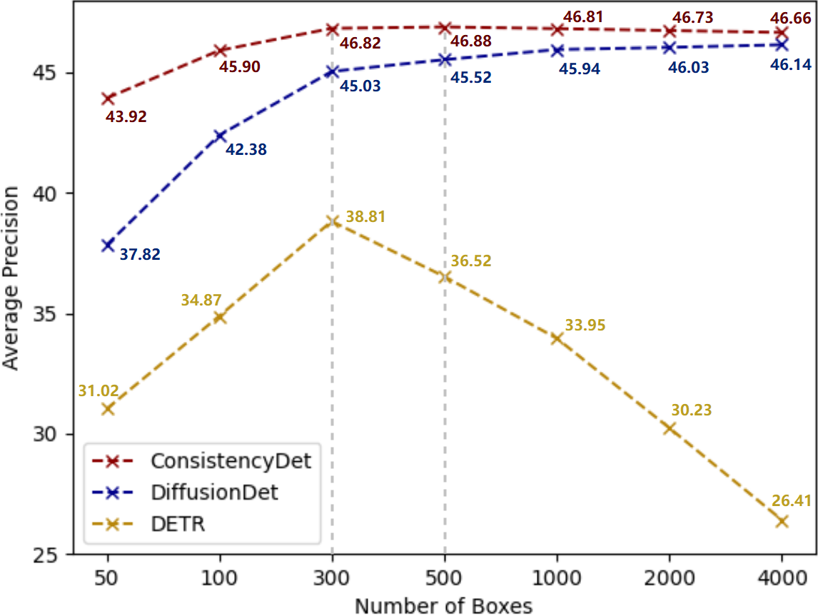
Figure 5: Performance comparisons with dynamic boxes. More proposal boxes in inference lead to accuracy improvement at first and tend towards stability for both ConsistencyDet and DiffusionDet, while causing a degradation in DETR. Furthermore, ConsistencyDet outperforms DiffusionDet for all these cases. Here, the results of AP are all percentage data (%).

Progressive refinement. For both training and inference, the number of proposal boxes is fixed at 500 at each sampling time step. In the MS-COCO dataset, ConsistencyDet demonstrates a stable performance enhancement as the number of sampling time steps increases from 1 to 10, as illustrated in Fig. 6. For instance, the AP for ConsistencyDet increases from 45.73% at a single time step ($T\!\!=\!\!1$) to 46.88% at ten time steps ($T\!\!=\!\!10$), marking an improvement of 1.15% in AP. This increment indicates that ConsistencyDet is capable of achieving higher accuracy with an optimal number of sampling time steps.

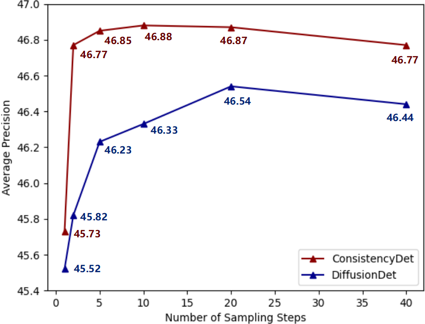
Figure 6: Performance analysis of progressive refinement. ConsistencyDet is evaluated with varied sampling time steps. It is trained on the MS-COCO dataset with ResNet-50 as the backbone, using 500 proposal boxes for training and evaluation at each sampling time step, and the number of total time steps $T=40$. Simultaneously, it is compared with DiffusionDet with the same assignments, except $T=1000$.

Sampling step. As depicted in Fig. 7, the sampling phase starts with the initialization of noised boxes at the $t$-th time step, with the noise addition protocol. These noised boxes are then put into the model to generate predictions. The detection decoder predicts the category scores and box coordinates of the current step. An initial filtration process ensues, whereby only the bounding boxes surpassing a predetermined confidence threshold are preserved. Under the theoretical guidance of the Consistency Model, noised boxes are predicted, optimized and filtered for the next time step. At the end of each time step, additional proposals are supplemented by the Box-renewal operation, ensuring the total amount of noise boxes reaches $n_{p}=500$ for the next iteration. In the final time step, NMS is applied to refine the results. By comparing the detection results in Fig. 7(f), it is evident that ConsistencyDet performs better than DiffusionDet, with more precise borders.

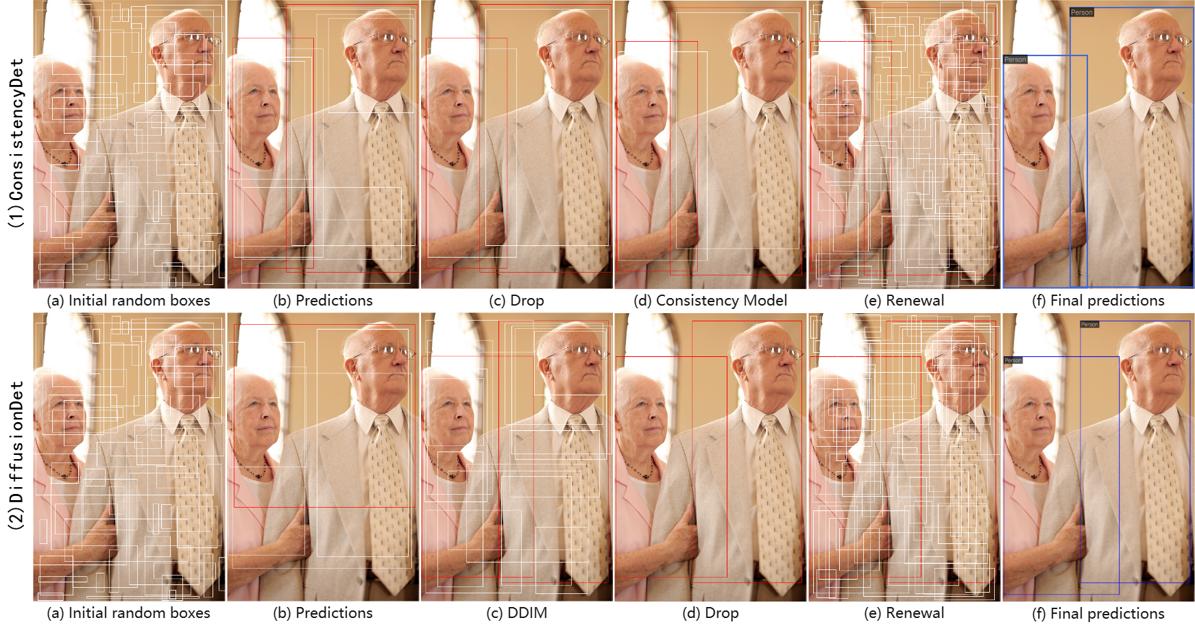
Figure 7: A comparison of the visual reasoning process with one typical sampling step between ConsistencyDet and DiffusionDet. We selected a sample image from the COCO 2017 val set for testing with both ConsistencyDet and DiffusionDet. The initial noised boxes or verified boxes with low confidence are marked in white, while the boxes with high confidence are marked in red and the final predictions are marked in blue.

Parameter selection for significance. Given the disparity in dataset attributes between MS-COCO and LVIS [28], they exhibit different sensitivities to noise. For the optimization of ConsistencyDet on each dataset, it is essential to conduct comparative analyses to ascertain the ideal setting for parameter $\sigma_{max}$. By calibrating this parameter, the model’s capacity to process noise can be fine-tuned, thereby facilitating its adaptation to the unique demands of each dataset and augmenting its efficacy across various contexts. This targeted adjustment plays a pivotal role in customizing the model’s performance for specific applications. The empirical outcomes, utilizing a ResNet-50 backbone with varying values of $\sigma_{max}$, are delineated in Table II.

TABLE II: Selecting the optimal $\sigma_{max}$ for COCO 2017 and LVIS v1.0 val set.

$\sigma_{max}$	AP	AP50	AP75	AP	AP50	AP75​
		​​COCO​​			​LVIS​
20	46.3	65.1	50.7	-	-	-
40	46.9	65.7	51.3	30.4	42.7	31.8
60	46.1	64.8	50.0	32.2	45.1	33.7
80	45.8	64.9	49.3	30.2	42.6	31.6

Results of AP ​​/​​ AP₅₀ ​​/​​ AP₇₅ are all percentage data (%).

Bold fonts indicate the best performance.

4.3 Simulation analysis

The performance of ConsistencyDet is evaluated against other state-of-the-art detector models [47, 13, 11, 10, 14] on the MS-COCO and LVIS datasets. The following provides an analysis of the simulation results.

TABLE III: Performance comparison of different object detectors on the COCO 2017 val set.

Method	AP	AP50	AP75	APs	APm	APl
Res-Net50
RetinaNet	38.7	58.0	41.5	23.3	42.3	50.3
Faster R-CNN	40.2	61.0	43.8	24.2	43.5	52.0
Cascade R-CNN	44.3	62.2	48.0	26.6	47.7	57.7
DETR	42.0	62.4	44.2	20.5	45.8	61.1
Deformable DETR	43.8	62.6	47.7	26.4	47.1	58.0
Sparse R-CNN	45.0	63.4	48.2	26.9	47.2	59.5
DiffusionDet (1 step)	45.5	65.1	48.7	27.5	48.1	61.2
DiffusionDet (4 step)	46.1	66.0	49.2	28.6	48.5	61.3
DiffusionDet (8 step)	46.2	66.4	49.5	28.7	48.5	61.5
ConsistencyDet	46.9	65.7	51.3	30.2	50.2	61.0
Res-Net101
RetinaNet	40.4	60.2	43.2	24.0	44.3	52.2
Faster R-CNN	42.0	62.5	45.9	25.2	45.6	54.6
Cascade R-CNN	45.5	63.7	49.9	27.6	49.2	59.1
DETR	43.5	63.8	46.4	21.9	48.0	61.8
Sparse R-CNN	46.4	64.6	49.5	28.3	48.3	61.6
DiffusionDet (1 step)​	46.6	66.3	50.0	30.0	49.3	62.8
DiffusionDet (4 step)​	46.9	66.8	50.4	30.6	49.5	62.6
DiffusionDet (8 step)​	47.1	67.1	50.6	30.2	49.8	62.7
ConsistencyDet	47.2	66.8	50.9	31.3	50.4	62.3
Swin-base
Cascade R-CNN	51.9	70.9	56.5	35.4	55.2	51.9
Sparse R-CNN	52.0	72.2	57.0	35.8	55.1	52.0
DiffusionDet (1 step)​	52.3	72.7	56.3	34.8	56.0	52.3
DiffusionDet (4 step)​	52.7	73.5	56.8	36.1	56.0	68.9
DiffusionDet (8 step)​	52.8	73.6	56.8	36.1	56.2	68.8
ConsistencyDet	53.0	73.2	57.6	36.5	57.2	68.4

Results of the above evaluation metrics are all percentage data (%).

Bold font indicates the best performance while italic font indicates the second best.

MS-COCO. The performance metrics of various detectors are compiled in Table III. ConsistencyDet, utilizing a ResNet-50 backbone, attains an AP of 46.9%, thereby outperforming established methodologies such as Faster R-CNN, RetinaNet, DETR, Sparse R-CNN, and DiffusionDet (with different sampling time steps). With the scaling up to a ResNet-101 backbone, ConsistencyDet’s performance is further enhanced, achieving an AP of 47.2%, which exceeds that of the aforementioned strong baselines. Moreover, when equipped with the Swin-base backbone [26] and pretrained on ImageNet-21k [42], ConsistencyDet reaches an impressive AP of 53.0%, eclipsing all the compared detectors. However, it should be noted that the proposed DiffusionDet exhibits the most robust overall performance, albeit with marginally lower results than the other detectors on specific metrics.

TABLE IV: Performance comparison of different object detectors on LVIS v1.0 val set.

Method	AP	AP50	AP75	APs	APm	APl	APr	APc	APf
Res-Net50
Faster R-CNN	25.2	40.6	26.9	18.5	32.2	37.7	16.4	23.4	31.1
Cascade R-CNN	29.4	41.4	30.9	20.6	37.5	44.3	20.0	27.7	35.4
Sparse R-CNN	29.2	41.0	30.7	20.7	36.9	44.2	20.6	27.7	34.6
DiffusionDet(1step)	30.4	42.8	31.8	20.6	38.6	47.6	23.5	28.1	36.0
DiffusionDet(4step)	31.8	45.0	33.2	22.5	39.6	48.3	24.8	29.3	37.6
DiffusionDet(8step)	31.9	45.3	33.1	22.8	40.2	48.1	24.0	29.5	38.1
ConsistencyDet	32.2	45.1	33.7	23.1	40.4	47.7	24.3	30.1	38.0
Res-Net101
Faster R-CNN	27.2	42.9	29.1	20.3	35	40.4	18.8	25.4	31.1
Cascade R-CNN	31.6	43.8	33.4	22.3	39.7	47.3	23.9	29.8	35.4
Sparse R-CNN	30.1	42.0	31.9	21.3	38.5	45.6	23.5	27.5	34.6
DiffusionDet(1step)	31.9	44.6	33.1	21.6	40.3	49.0	23.4	30.5	36.0
DiffusionDet(4step)	32.9	46.5	34.3	23.3	41.1	49.9	24.2	31.3	37.6
DiffusionDet(8step)	33.5	47.3	34.7	23.6	41.9	49.8	24.8	32.0	39.0
ConsistencyDet	33.1	46.1	34.8	22.9	41.5	49.4	24.9	31.2	38.7
Swin-base
DiffusionDet(1step)	40.6	54.8	42.7	28.3	50.0	61.6	33.6	39.8	44.6
DiffusionDet(4step)	41.9	57.1	44.0	30.3	50.6	62.3	34.9	40.7	46.3
DiffusionDet(8step)	42.1	57.8	44.3	31.0	51.3	62.5	34.3	41.0	46.7
ConsistencyDet	42.4	57.1	44.9	30.3	51.5	63.4	34.9	41.5	46.8

Results of the above evaluation metrics are all percentage data (%).

Bold font indicates the best performance while italic font indicates the second best performance.

LVIS v1.0. Table IV presents a comparative analysis of object detection performance between ConsistencyDet and various other detection models. Reproductions of Faster R-CNN and Cascade R-CNN yielded AP scores of 25.2% and 27.2% with a ResNet-50 backbone, and 29.4% and 31.6% with a ResNet-101 backbone, respectively. ConsistencyDet, employing a ResNet-50 backbone, achieved an AP of 32.2%, exceeding the performance of established methods such as Faster R-CNN, RetinaNet, DETR, and Sparse R-CNN, while also remaining competitive with DiffusionDet. As the backbone is scaled up, ConsistencyDet exhibits consistent performance enhancements. With the ResNet-101 backbone, ConsistencyDet reaches an AP of 33.1%, surpassing robust baselines including Faster R-CNN, RetinaNet, DETR, Sparse R-CNN, and DiffusionDet at a quarter step, although it falls slightly behind DiffusionDet at an eight-step iteration. Furthermore, when leveraging the Swin-base backbone [26] pretrained on ImageNet-21k [42], ConsistencyDet achieves a significant AP of 42.4%, outstripping all the aforementioned baselines and establishing new benchmarks for models such as Faster R-CNN, RetinaNet, DETR, Sparse R-CNN, and DiffusionDet.

4.4 Ablation Study

Comprehensive ablation studies were conducted to elucidate the characteristics of the proposed ConsistencyDet model on the MS-COCO and LVIS v1.0 datasets. These simulations utilized a ResNet-50 architecture equipped with a FPN as the primary backbone, with no further modifications or enhancements specified.

Box-renewal threshold. The left column of Table V illustrates the impact of the score threshold, denoted as B_th, on the Box-renewal process. A threshold value of 0.0 implies that Box-renewal is not employed. According to the evaluation on the COCO 2017 validation set, employing a threshold of 0.98 marginally outperforms other threshold settings.

It is important to note that the optimal threshold selection may exhibit slight variations when coupled with different backbone architectures in the dataset, as evidenced in the middle column of Table VI. To ensure the robustness and generalizability of the code during the testing phase, unified parameters were established, and the corresponding AP is documented in the right column of Table VI.

TABLE V: Optimal choices for the thresholds for the Box-renewal and NMS operation.

Bth	AP	AP50	AP75	Nth	AP	AP50	AP75
-	-	-	-	0.5	46.5	66.6	50.0
0.9	46.5	65.5	50.9	0.6	46.8	66.0	50.8
0.98	46.9	65.7	51.3	0.64	46.9	65.7	51.3
1.0	46.7	65.6	51.2	0.7	46.6	64.8	51.5

Results of AP ​/​ AP₅₀ ​/​ AP₇₅ are all percentage data (%).

Bold fonts indicate the best performance.

NMS threshold. The right column of Table V delineates the effects of varying the NMS score threshold, represented as N_th, on the AP. Setting the threshold to 0.0 signifies the absence of any NMS procedure. An analysis of the COCO 2017 validation set suggests that a threshold of 0.64 yields a performance that is modestly superior relative to the other thresholds investigated. Table VI presents the AP scores for ConsistencyDet on the LVIS v1.0 dataset, utilizing a Box-renewal score threshold (B_th) of 0.85 and an NMS score threshold (N_th) of 0.60. These configurations result in satisfactory performance outcomes.

TABLE VI: Optimal choices for Box-renewal threshold and score threshold across different datasets and backbones.

Dataset	Backbone	Bth​​​	Nth​​​	AP	Bth​​​	Nth​​​	AP
COCO	ResNet-50	0.98	0.64	46.9	0.98	0.64	46.9
	ResNet-101	0.85	0.60	47.2	0.98	0.64	47.0
	Swin-Base	0.98	0.62	53.0	0.98	0.64	52.8
LVIS	ResNet-50	0.85	0.60	32.2	0.85	0.60	32.2
	ResNet-101	0.85	0.60	33.1	0.85	0.60	33.1
	Swin-Base	0.85	0.60	42.4	0.85	0.60	42.4

Results of AP are all percentage data (%).

Bold font indicates the best performance.

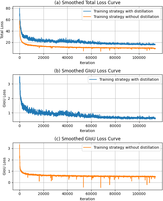
Figure 8: Smoothed loss curves of ConsistencyDet via different training strategies. (a) The comparison of the total loss curves between two training strategies. (b) Smoothed GIoU loss curve of training strategy with distillation. (c) Smoothed GIoU loss curve of independent training strategy without distillation.

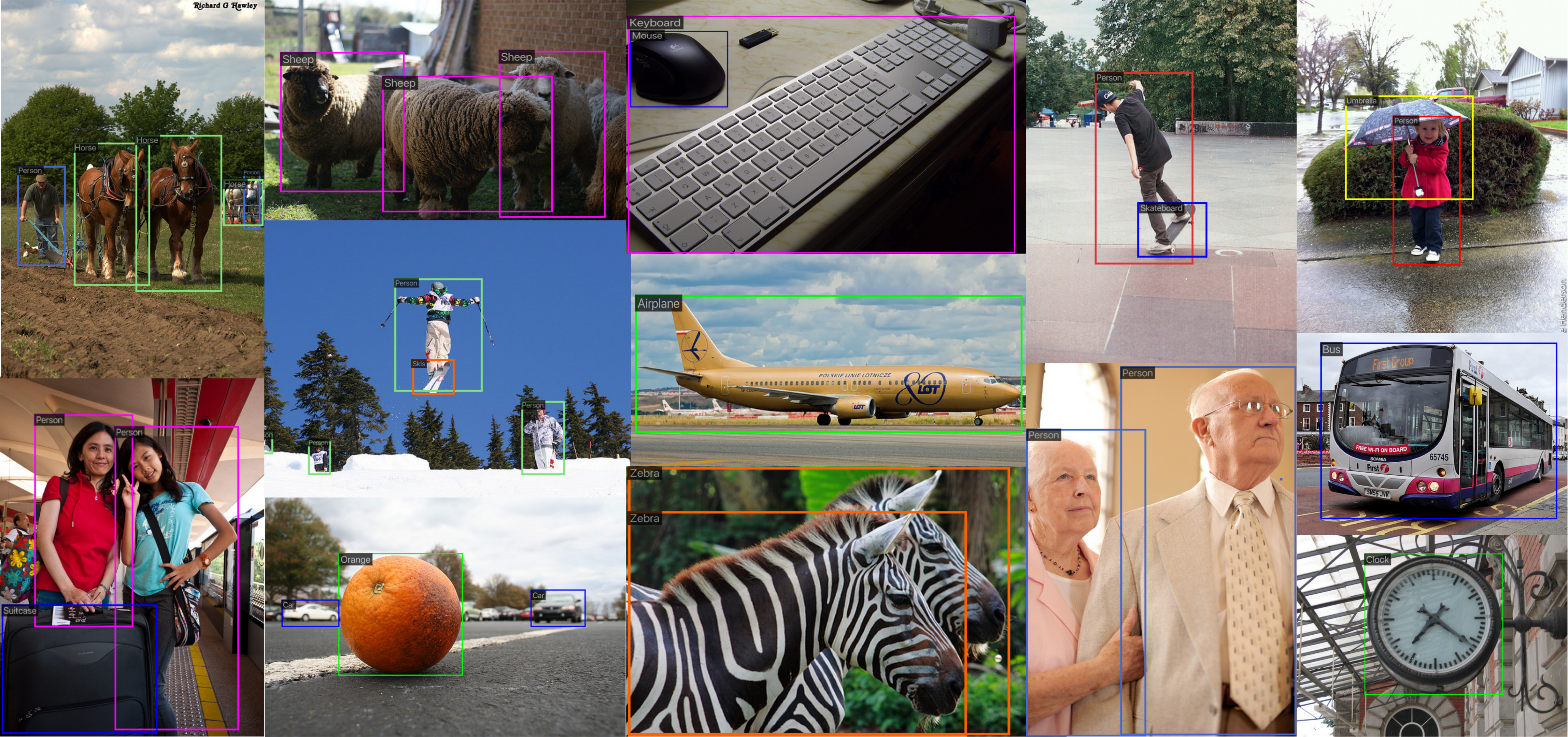
Figure 9: Typical instances of detected objects by the proposed ConsistencyDet. The objects in these images are detected with correct categories and accurate borders.

Training strategy. Algorithm 4 provides two training strategies, differentiated by whether to utilize a pre-trained DiffusionDet model for the distillation training of ConsistencyDet. In Fig. 8, the loss curves of these two strategies are compared in the coordinate system. Both are trained with 4 GPUs, and the batch size is set to 2 for each GPU. The training process adopts Res-Net50 as the backbone and is conducted on the MS-COCO dataset. While DiffusionDet could, in theory, achieve better results with an adequate number of denoising time steps, the complexity of its operational steps presents challenges in effective training, which in turn limits its performance in practice. Hence, our experimental efforts primarily focus on the training strategy of the Consistency Model in isolation.

From Fig. 8 (b) and (c), it is evident that employing distillation training can effectively mitigate the issue of outliers encountered during the training process. At the latter half of the timeline, the stochastic nature introduced by noise may sometimes lead to unreasonable values of box coordinates, where the top-left coordinates are smaller than the bottom-right coordinates. This illogical issue results in negative GIoU loss values, potentially causing the model to converge in an erroneous direction, which could pose potential risks. Therefore, the introduction of distillation brings corresponding benefits.

Since the predictions of current DiffusionDet still have a big gap with GT information, if the position information of the boxes predicted by DiffusionDet is used as the reference information from the origin of the timeline, this operation inevitably leads to inadequate guidance in the training process of ConsistencyDet, and results in a larger total loss with poor performance, shown as Fig. 8 (a). Therefore, after comprehensive consideration, this work adopts the independent training strategy for the training process which achieves better results. Also, the aforementioned illogical issue can be restrained with the conservative limitation of value ranges.

Accuracy vs. speed. Table VII compares the inference speeds of ConsistencyDet and DiffusionDet, both employing a ResNet-50 backbone, on the COCO 2017 validation set. The runtime performance was measured using a single NVIDIA RTX 3080 GPU and a batch size of one. DiffusionDet’s evaluation includes various sampling time steps ($t_{ss}=20,40,60,100$) with a total time step of $T=1000$, from which AP and frames per second (FPS) were recorded. ConsistencyDet was tested at total time steps of $t_{ss}=2$ and $10$ with $T=40$. The experiment outcomes reveal that ConsistencyDet not only achieves a substantial enhancement in inference speed when compared to DiffusionDet but also demonstrates a modest improvement of 0.4% in AP.

TABLE VII: Accuracy vs. speed comparison of ConsistencyDet and DiffusionDet at different sampling time steps.

Model	$T$	$n_{ss}$	AP	FPS
DiffusionDet	1000	20	46.5	0.954
	1000	40	46.4	0.473
	1000	60	46.5	0.309
ConsistencyDet	40	2	46.8	6.892
	40	10	46.9	1.783

Results of AP are all percentage data (%).

Bold font indicates the best performance while italic font indicates the second best.

In this study, we introduce a novel object detection framework that incorporates the Consistency Model, which is compatible with commonly utilized backbone and head architectures. This framework does not impose special requirements on the network structures. The proposed ConsistencyDet demonstrated superior overall performance compared to other well-established detectors. Fig. 9 showcases the visualizations of typical instances where ConsistencyDet has accurately detected objects with precise boundaries and correct category annotations. Although there is still a performance gap when compared to top-performing detectors cited in references [48, 49, 50], we anticipate that the performance of DiffusionDet could be further enhanced through its integration with specially designed architectures.

Despite its promising performance, ConsistencyDet is not without limitations. Its detection accuracy for larger objects is marginally lower than that of DiffusionDet and DETR when using certain backbones, partly due to the noise addition strategy not fully taking into account the scale of the objects. While it operates faster than DiffusionDet, there remains a need for further efficiency improvements to meet the demands of real-time applications.

5 Conclusions

In this work, we have introduced a novel object detection paradigm, ConsistencyDet, which conceptualizes object detection as a denoising diffusion process evolving from noisy boxes to precise targets. The proposed ConsistencyDet leverages the Consistency Model for object detection and presents an innovative strategy for the addition of noise and denoising. A key feature of the ConsistencyDet model is its self-consistency, which ensures that noise information at any temporal stage can be directly mapped back to the origin on the coordinate axis, thus significantly boosting the algorithm’s computational efficiency.

Through simulations conducted on standard object detection benchmarks, it has been confirmed that ConsistencyDet achieves competitive performance in comparison to other established detectors. In a head-to-head comparison with DiffusionDet, ConsistencyDet displays efficient processing across these datasets. Notably, with the selection of optimal sampling time steps for both models, ConsistencyDet demonstrates substantial gains in computational efficiency over DiffusionDet. This result is a testament to the self-consistency feature intrinsic to ConsistencyDet.

Prospective enhancements to ConsistencyDet are manifold and could serve to further refine the approach. Future work may include: (1) Revising noise addition and denoising techniques to improve detection accuracy, particularly for larger objects. (2) Expanding the performance capabilities of the Consistency Model in object detection tasks, potentially through the implementation of training strategies that incorporate knowledge distillation from well-trained Diffusion Models. (3) Enhancing computational efficiency by simplifying the operational steps in the model. (4) Extending the proposed noise addition and denoising framework to additional domains, such as image segmentation and object tracking.

References

- [1] Z. Zou, K. Chen, Z. Shi, Y. Guo, and J. Ye, “Object detection in 20 years: A survey,” Proceedings of the IEEE, vol. 111, no. 3, pp. 257–276, 2023.
- [2] H. Ghahremannezhad, H. Shi, and C. Liu, “Object detection in traffic videos: A survey,” IEEE Transactions on Intelligent Transportation Systems, vol. 24, no. 7, pp. 6780–6799, 2023.
- [3] G. Cheng, X. Yuan, X. Yao, K. Yan, Q. Zeng, X. Xie, and J. Han, “Towards large-scale small object detection: Survey and benchmarks,” IEEE Transactions on Pattern Analysis and Machine Intelligence, vol. 45, no. 11, pp. 13 467–13 488, 2023.
- [4] Z. Tian, B. Zhang, H. Chen, and C. Shen, “Instance and panoptic segmentation using conditional convolutions,” IEEE Transactions on Pattern Analysis and Machine Intelligence, vol. 45, no. 1, pp. 669–680, 2023.
- [5] T. Zhang, J. Lian, J. Wen, and C. L. P. Chen, “Multi-person pose estimation in the wild: Using adversarial method to train a top-down pose estimation network,” IEEE Transactions on Systems, Man, and Cybernetics: Systems, vol. 53, no. 7, pp. 3919–3929, 2023.
- [6] S. Mathe and C. Sminchisescu, “Actions in the eye: Dynamic gaze datasets and learnt saliency models for visual recognition,” IEEE Transactions on Pattern Analysis and Machine Intelligence, vol. 37, no. 7, pp. 1408–1424, 2015.
- [7] Y. Zhang, Y. Liang, J. Leng, and Z. Wang, “Scgtracker: Spatio-temporal correlation and graph neural networks for multiple object tracking,” Pattern Recognition, vol. 149, p. 110249, 2024.
- [8] T. Truong and S. Yanushkevich, “Visual relationship detection for workplace safety applications,” IEEE Transactions on Artificial Intelligence, vol. 5, no. 2, pp. 956–961, 2024.
- [9] R. Girshick, “Fast r-cnn,” in Proceedings of the IEEE international conference on computer vision, 2015, pp. 1440–1448.
- [10] S. Ren, K. He, R. Girshick, and J. Sun, “Faster r-cnn: Towards real-time object detection with region proposal networks,” Advances in neural information processing systems, vol. 28, 2015.
- [11] T.-Y. Lin, P. Goyal, R. Girshick, K. He, and P. Dollár, “Focal loss for dense object detection,” in Proceedings of the IEEE international conference on computer vision, 2017, pp. 2980–2988.
- [12] J. Redmon, S. Divvala, R. Girshick, and A. Farhadi, “You only look once: Unified, real-time object detection,” in Proceedings of the IEEE conference on computer vision and pattern recognition, 2016, pp. 779–788.
- [13] N. Carion, F. Massa, G. Synnaeve, N. Usunier, A. Kirillov, and S. Zagoruyko, “End-to-end object detection with transformers,” in Proceedings of the European conference on computer vision, 2020, pp. 213–229.
- [14] P. Sun, R. Zhang, Y. Jiang, T. Kong, C. Xu, W. Zhan, M. Tomizuka, L. Li, Z. Yuan, C. Wang et al., “Sparse r-cnn: End-to-end object detection with learnable proposals,” in Proceedings of the IEEE/CVF conference on computer vision and pattern recognition, 2021, pp. 14 454–14 463.
- [15] P. Gao, M. Zheng, X. Wang, J. Dai, and H. Li, “Fast convergence of detr with spatially modulated co-attention,” in Proceedings of the IEEE/CVF international conference on computer vision, 2021, pp. 3621–3630.
- [16] F. Li, H. Zhang, S. Liu, J. Guo, L. M. Ni, and L. Zhang, “Dn-detr: Accelerate detr training by introducing query denoising,” in Proceedings of the IEEE/CVF Conference on Computer Vision and Pattern Recognition, 2022, pp. 13 619–13 627.
- [17] P. Dhariwal and A. Nichol, “Diffusion models beat gans on image synthesis,” Advances in neural information processing systems, vol. 34, pp. 8780–8794, 2021.
- [18] F.-A. Croitoru, V. Hondru, R. T. Ionescu, and M. Shah, “Diffusion models in vision: A survey,” IEEE Transactions on Pattern Analysis and Machine Intelligence, vol. 45, no. 9, pp. 10 850–10 869, 2023.
- [19] Z. Yuan, C. Hao, R. Zhou, J. Chen, M. Yu, W. Zhang, H. Wang, and X. Sun, “Efficient and controllable remote sensing fake sample generation based on diffusion model,” IEEE Transactions on Geoscience and Remote Sensing, vol. 61, pp. 1–12, 2023.
- [20] E. A. Brempong, S. Kornblith, T. Chen, N. Parmar, M. Minderer, and M. Norouzi, “Denoising pretraining for semantic segmentation,” in Proceedings of the IEEE/CVF conference on computer vision and pattern recognition, 2022, pp. 4175–4186.
- [21] S. Chen, P. Sun, Y. Song, and P. Luo, “Diffusiondet: Diffusion model for object detection,” in Proceedings of the IEEE/CVF International Conference on Computer Vision, 2023, pp. 19 830–19 843.
- [22] Y. Song, P. Dhariwal, M. Chen, and I. Sutskever, “Consistency models,” 2023.
- [23] Y. Song, J. Sohl-Dickstein, D. P. Kingma, A. Kumar, S. Ermon, and B. Poole, “Score-based generative modeling through stochastic differential equations,” arXiv preprint arXiv:2011.13456, 2020.
- [24] J. Ho, A. Jain, and P. Abbeel, “Denoising diffusion probabilistic models,” Advances in neural information processing systems, vol. 33, pp. 6840–6851, 2020.
- [25] K. He, X. Zhang, S. Ren, and J. Sun, “Deep residual learning for image recognition,” in Proceedings of the IEEE conference on computer vision and pattern recognition, 2016, pp. 770–778.
- [26] Z. Liu, Y. Lin, Y. Cao, H. Hu, Y. Wei, Z. Zhang, S. Lin, and B. Guo, “Swin transformer: Hierarchical vision transformer using shifted windows,” in Proceedings of the IEEE/CVF international conference on computer vision, 2021, pp. 10 012–10 022.
- [27] T.-Y. Lin, M. Maire, S. Belongie, J. Hays, P. Perona, D. Ramanan, P. Dollár, and C. L. Zitnick, “Microsoft coco: Common objects in context,” in Proceedings of the European conference on computer vision, 2014, pp. 740–755.
- [28] A. Gupta, P. Dollar, and R. Girshick, “Lvis: A dataset for large vocabulary instance segmentation,” in Proceedings of the IEEE/CVF conference on computer vision and pattern recognition, 2019, pp. 5356–5364.
- [29] J. Austin, D. D. Johnson, J. Ho, D. Tarlow, and R. Van Den Berg, “Structured denoising diffusion models in discrete state-spaces,” Advances in Neural Information Processing Systems, vol. 34, pp. 17 981–17 993, 2021.
- [30] V. Popov, I. Vovk, V. Gogoryan, T. Sadekova, and M. Kudinov, “Grad-tts: A diffusion probabilistic model for text-to-speech,” in International Conference on Machine Learning, 2021, pp. 8599–8608.
- [31] L. Wu, C. Gong, X. Liu, M. Ye, and Q. Liu, “Diffusion-based molecule generation with informative prior bridges,” Advances in Neural Information Processing Systems, vol. 35, pp. 36 533–36 545, 2022.
- [32] H. Cao, C. Tan, Z. Gao, Y. Xu, G. Chen, P.-A. Heng, and S. Z. Li, “A survey on generative diffusion models,” IEEE Transactions on Knowledge and Data Engineering, 2024.
- [33] C. H. Lampert, H. Nickisch, and S. Harmeling, “Attribute-based classification for zero-shot visual object categorization,” IEEE Transactions on Pattern Analysis and Machine Intelligence, vol. 36, no. 3, pp. 453–465, 2014.
- [34] J. Song, C. Meng, and S. Ermon, “Denoising diffusion implicit models,” arXiv preprint arXiv:2010.02502, 2020.
- [35] G. Hinton, O. Vinyals, and J. Dean, “Distilling the knowledge in a neural network,” Computer Science, vol. 14, no. 7, pp. 38–39, 2015.
- [36] T. Garbay, O. Chuquimia, A. Pinna, H. Sahbi, and B. Granado, “Distilling the knowledge in cnn for wce screening tool,” in Proceedings of the 2019 Conference on Design and Architectures for Signal and Image Processing (DASIP), 2019.
- [37] T.-Y. Lin, P. Dollár, R. Girshick, K. He, B. Hariharan, and S. Belongie, “Feature pyramid networks for object detection,” in Proceedings of the IEEE conference on computer vision and pattern recognition, 2017, pp. 2117–2125.
- [38] T. Amit, T. Shaharbany, E. Nachmani, and L. Wolf, “Segdiff: Image segmentation with diffusion probabilistic models,” arXiv preprint arXiv:2112.00390, 2021.
- [39] M. Everingham, L. Van Gool, C. K. Williams, J. Winn, and A. Zisserman, “The pascal visual object classes (voc) challenge,” International journal of computer vision, vol. 88, pp. 303–338, 2010.
- [40] S. Shao, Z. Zhao, B. Li, T. Xiao, G. Yu, X. Zhang, and J. Sun, “Crowdhuman: A benchmark for detecting human in a crowd,” arXiv preprint arXiv:1805.00123, 2018.
- [41] H. Rezatofighi, N. Tsoi, J. Gwak, A. Sadeghian, I. Reid, and S. Savarese, “Generalized intersection over union: A metric and a loss for bounding box regression,” in Proceedings of the IEEE/CVF conference on computer vision and pattern recognition, 2019, pp. 658–666.
- [42] J. Deng, W. Dong, R. Socher, L.-J. Li, K. Li, and F.-F. Li, “Imagenet: A large-scale hierarchical image database,” in 2009 IEEE conference on computer vision and pattern recognition, 2009, pp. 248–255.
- [43] X. Glorot and Y. Bengio, “Understanding the difficulty of training deep feedforward neural networks,” in Proceedings of the thirteenth international conference on artificial intelligence and statistics, 2010, pp. 249–256.
- [44] I. Loshchilov and F. Hutter, “Decoupled weight decay regularization,” arXiv preprint arXiv:1711.05101, 2017.
- [45] H. Zhang, M. Cisse, Y. N. Dauphin, and D. Lopez-Paz, “mixup: Beyond empirical risk minimization,” arXiv preprint arXiv:1710.09412, 2017.
- [46] Z. Ge, S. Liu, F. Wang, Z. Li, and J. Sun, “Yolox: Exceeding yolo series in 2021,” arXiv preprint arXiv:2107.08430, 2021.
- [47] Z. Cai and N. Vasconcelos, “Cascade r-cnn: High quality object detection and instance segmentation,” IEEE transactions on pattern analysis and machine intelligence, vol. 43, no. 5, pp. 1483–1498, 2019.
- [48] W. Wang, J. Dai, Z. Chen, Z. Huang, Z. Li, X. Zhu, X. Hu, T. Lu, L. Lu, H. Li, X. Wang, and Y. Qiao, “Internimage: Exploring large-scale vision foundation models with deformable convolutions,” in Proceedings of the IEEE/CVF Conference on Computer Vision and Pattern Recognition, 2023, pp. 14 408–14 419.
- [49] Z. Liu, H. Hu, Y. Lin, Z. Yao, Z. Xie, Y. Wei, J. Ning, Y. Cao, Z. Zhang, L. Dong, F. Wei, and B. Guo, “Swin transformer v2: Scaling up capacity and resolution,” in Proceedings of the IEEE conference on computer vision and pattern recognition, 2022, pp. 11 999–12 009.
- [50] Z. Zong, G. Song, and Y. Liu, “Detrs with collaborative hybrid assignments training,” in Proceedings of the IEEE international conference on computer vision, 2023, pp. 6725–6735.