Coupling nanoscopic tomography and micromagnetic modelling to assess the stability of geomagnetic recorders

Abstract

The recording of planetary magnetic fields is often attributed to uniformly-magnetised nanoscopic iron oxides, called single-domain (SD). Yet, the main magnetic constituents of rocks are more complex, non-uniformly magnetised grains in single or multi-vortex states. We know little about their behaviour due to limitations in defining their precise shape and internal magnetic structure. We propose a novel approach combining non-destructive synchrotron-based ptychographic nanotomography with micromagnetic modelling to explore the magnetic stability of remanence-bearing minerals. Applied to a microscopic rock sample, we identified hundreds of nanoscopic grains of magnetite/maghemite with diverse morphologies. For some grains, shape irregularities near the transition from SD to the single-vortex state allow for multiple domain states, some unstable and unable to record the field for significant periods. Additionally, some other grains exhibit temperature-dependent occupancy probabilities, potentially hampering experiments to recover the intensity of past magnetic fields.

Keywords: nano-tomography, micromagnetic modelling, vortex state

Introduction

Measuring the magnetic properties and identifying the magnetic minerals in rocks is essential to palaeomagnetism, which studies Earth’s magnetic field strength and direction throughout the planet’s geological history [1]. While directional palaeomagnetic data is the only quantitative measurement that allows geoscientists to study palaeoconfigurations of ancient continental landmasses [2], databases of the past magnetic field strength (palaeointensity) [3] provide links to the complex magnetohydrodynamic processes occurring deep in Earth’s core [4, 5, 6]. Quantifying the magnetic phases in rocks also provides essential information on globally scaled geological/climate events [7]. Rocks usually contain a mixture of magnetic particles in various sizes, including very stable nanoscopic uniformly magnetised grains (said to be in a single-domain (SD) state) and larger non-uniformly magnetised grains, either in pseudo-single-domain (PSD) or in multi-domain (MD) states. The palaeomagnetic theory is mainly based on Néel[8] ferromagnetic theory for SD grains, which relies on the capacity of these particles to retain their original remanence for billions of years but accounts only for a small proportion of magnetic particles contained within a typical palaeomagnetic sample.

Palaeomagnetic analysis of a samples’ magnetic mineralogy and stability is usually based on bulk magnetic measurements, often capable of detecting trace amounts of magnetic minerals. Although the data obtained through these analyses use statistical procedures to ensure their reliability, critical magnetic phenomena with geological/geophysical implications can sometimes be masked in bulk magnetic measurements. The complexity of natural geological materials and the diversity of composition/geometry of natural remanence carriers in rocks indicate that the conditions assumed by classical palaeomagnetic experiments can be far from ideal. A detailed understanding of the magnetic recording reliability requires a nanoscale interpretation of the magnetic fidelity of magnetic mineral grains.

Micromagnetic modelling, which explores the magnetic properties of a given grain (or a population of them) as a function of their size, shape, composition and temperature [9, 10], is an important tool that can bring a far greater understanding of the magnetic recording process. Micromagnetic calculations have revealed, for example, i) that PSD structures (also referred to as vortex states due to their magnetisation being dominated by single or multiple vorticity centres), which is probably the most common type of magnetic domain structure in natural iron oxides [11], often are capable of retaining their remanence for timescales longer than the age of the Solar System [12]; and ii) the theoretical discovery of a non-stable magnetic configuration in grain sizes beyond the SD threshold [13], which can produce unexpected magnetic properties (e.g, the reduction of coercivities and thermal stability) and has the potential to greatly affect palaeointensity data [14].

Particle size is a very important controller of domain state and, consequently, of magnetic stability [15], but geometry is also a critical factor. Although micromagnetic modelling of irregular particle morphologies through the discretization of three-dimensional finite element meshes is possible [10], most of the theoretical knowledge built on micromagnetics of iron oxides is based on regular euhedral crystalline habits [16, 9, 17, 12, 18, 14, 13]. Although natural processes can trigger regular crystal growth/alteration of iron oxides (such as biosynthesis of magnetite by magnetotatic bacteria [19, 20]), tomographic techniques of iron oxides bearing rocks very often reveal irregularly shaped grains [21, 11, 22]. Consequently, it is important to understand how these irregular morphologies of particles might affect their magnetic properties, especially for grains within the palaeomagnetically significant PSD threshold.

In this study, we introduce the use of Synchrotron-based Ptychographic X-ray Computed Nano-tomography (PXCT) [23] (Figure 1) to image the magnetic minerals within a microscopic sample of a Neoproterozoic remagnetised carbonate, and further model their micromagnetic behaviour through finite element numerical models. The primary remanence (acquired during pre-to-syn diagenetic conditions) of carbonate rocks is very often substituted by a secondary chemical remanence (CRM) [24, 25] when new magnetic minerals grow or are chemically altered below their respective Curie temperature (Tc) [15]. These processes result in magnetic grains with a wide range of sizes and shapes, most of them within the SD/PSD grain size range, making them a target for micromagnetic studies of individual particles at the micro/nanoscopic scale. To image them, PXCT was chosen for being a non-destructive coherent diffractive imaging method that allows a quantitative mapping of the tridimensional electron density distribution of the specimen at unmatched nanoscale resolution [26, 27]. Our results provide new insights into the magnetic properties of natural remanence carriers in rocks and their thermomagnetic stability.

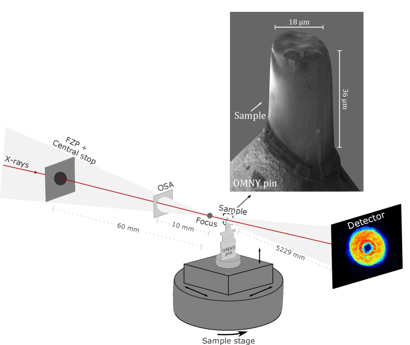
Figure 1: Experimental setup for the acquisition of PXCT data. X-rays are focused by a Fresnel Zone Plate (FZP), in combination with a central stop and an order sorting aperture (OSA), to define the illumination. The radiation reaches the microscopic pillar sample, mounted at the tip of an OMNY (tOMography Nano crYo) pin [28]. A scanning electron microscopy (SEM) image of the sample is shown in the upper corner of the figure. The sample stage allows a three-axial movement of the sample on top of a rotation to perform raster scans at different angles with respect to the X-ray beam. Diffraction patterns at each scan position are captured by a pixelated detector. The components sketched in this figure are not to scale. Details can be found in the text (or in the Supplementary File).

Results

Nano-tomography

The processed tomograms representing the 3D electron density distribution of the specimen resulted in artefact-free volumes with a voxel size of $34.84\ \text{nm}$. An example is shown in Supplementary File, Figure S1a, while details about the PXCT measurements and data processing can be found in the Methods section and in the Supplementary File. By using the accumulated histogram distribution of all of the data and the natural breaks in the distribution (Supplementary File, Figure S1c), we have segmented five compositional classes (Supplementary File, Figure S1d, Table S1). Our interpretations of the imaged materials presented here are also supported by previous chemical/magnetic analyses performed by Bellon et al. [29].

The classes are named according to their increasing electron density (Figure 2). Class 1 yields the lowest electron density of $\mu=0.31\pm 0.11\ e^{-}\cdot\text{\r{A}}^{-3}$, also showing restricted volumetric occurrence. This material appears in small clusters within the sample (Figure 2a, green colour), also showing a spatial correlation to localised porosities. We attribute this class to organic matter, specifically to bitumen. The geological formation (from which our sample comes) is naturally enriched in hydrocarbons [30], as biodegradation of the organic matter is also considered partially responsible for the growth of authigenic ferromagnetic minerals. Natural bitumen density might vary depending on its formation and preservation, but the density of natural bitumens [31] has been reported to be $1.02-1.03\ \text{g/cm}^{3}$, which reflects an electron density (Equation 2) of $0.30-0.31\ e^{-}\cdot\text{\r{A}}^{-3}$.

Class 2 $(\mu=0.65\pm 0.08\ e^{-}\cdot\text{\r{A}}^{-3})$ material occupies a large volume of the sample (Figure 2a, yellowish colour), and it is interpreted as a phyllosilicate. Smectite-illite has been previously identified as a major mineralogical constituent of these samples, see Ref. [29], as their conversion process (smectite to illite) is believed to release iron that sequentially reacts with the available oxygen to form iron oxides [32, 33]. The density of such phyllosilicates will depend on their purity. Smectite’s (end member smectite, EMS, $<2.3\ \text{g/cm}^{3}$) transformation to illite might be partial (illite-rich mixed-layer clays, IML, $2.4-2.7\ \text{g/cm}^{3}$), or complete (end-member illite, EMI, $>2.7\ \text{g/cm}^{3}$) [34]. The spread distribution of Class 2 matches the expected density of a partial smectite-illitisation, as EMS and IML electron densities are between $0.69$ and $0.72\ e^{-}\cdot\text{\r{A}}^{-3}$ (respectively).

Classes 3 $(\mu=0.80\pm 0.01\ e^{-}\cdot\text{\r{A}}^{-3})$ and 4 $(\mu=0.88\pm 0.03\ e^{-}\cdot\text{\r{A}}^{-3})$ comprise the majority of the rock matrix and are interpreted, essentially, as calcium carbonates (Figure 2b). Class 3 matches the expected electron density of calcite $(\text{CaCO}_{3},0.81\ e^{-}\cdot\text{\r{A}}^{-3})$, while Class 4 matches that of dolomite $(\text{CaMg(CO}_{3}\text{)}_{2},0.85\ e^{-}\cdot\text{\r{A}}^{-3})$.

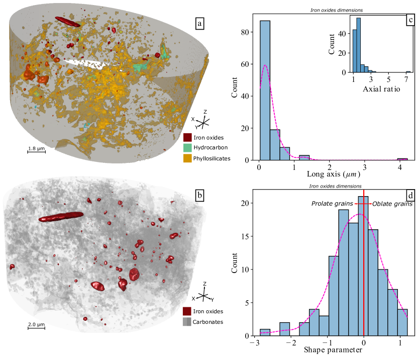
Figure 2: Reconstruction of the PXCT 3D electron density distribution after segmentation, highlighting different materials in (a) and (b). Most of the iron oxide grains have a major elongation axis between $80-600\ \text{nm}$ (c) and an axial ratio ($\text{P}_{1}/\text{P}_{3}$) $<2$. In (d), the shape parameter ($\epsilon$, revisit Equation 4) is quite scattered, showing a well-distributed population of triaxial ($\epsilon\approx 0$), prolate ($\epsilon<<0$) and oblate ($\epsilon>>0$) grains.

Class 5 gathers the highest mean electron densities of our sample $(\mu=1.08\pm 0.09\ e^{-}\cdot\text{\r{A}}^{-3})$, almost 20% larger than Class 4. The volumetric distribution of the material represented by this class is also quite distinct from the other ones, as these appear as individual grains spread in the matrix (Figure 2b). They also represent a wider electron density distribution, with values that reach as far as $1.24\ e^{-}\cdot\text{\r{A}}^{-3}$. We interpret this material as the iron oxide particles in our sample. The electron density upper limit of Class 5 was also observed for partially oxidised magnetite/maghemite in previous PXCT studies [35], but is slightly lower than expected from their theoretical densities. Several aspects could implicate such discrepancies, for example: (i) chemical impurities, crystalline imperfections and oxidation; (ii) density is size-dependent in nanomaterials, being lower/greater than a correspondent macrometric material depending on the lattice parameter [36]. The most likely reason though is related to the partial volume effect, i.e, for a given small volume the measured electron density has a large contribution from the voxels at the interface with its surrounding material, which can affect the final average density value. In our case, we have particles of a few hundred nanometers sampled with a 3D resolution, therefore a large proportion of the selected volume for density quantification may have a contribution from the density of the surrounding material. If the surrounding material has a lower density, the density will be underestimated. Partial volume effects have been considered before, e.g., in the segmentation of volumes of nanoporous material obtained by PXCT [37]. Prior applications of synchrotron-based techniques, specifically X-ray Fluorescence (XRF) and X-ray Absorption Near Edge Spectroscopy (XANES), have been utilised to identify magnetite/maghemite in a sister sample currently undergoing nano-tomographic analysis [29]. This additional evidence further supports our interpretation, as we follow the micromagnetic modelling of their properties.

Following the processing, segmentation, and mesh generation (refer to Methods for clarity), we have identified 118 distinct grains of iron oxides with varied shapes and sizes. Due to their high irregularity, we will discuss their sizes based on the ratios of the grains’ main axes ($\text{P}_{1}>\text{P}_{2}$ > $\text{P}_{3}$). More than 95% of the major axis have an elongation of $80-600\ \text{nm}$ (see Figure 2c), and 68% is smaller than $250\ \text{nm}$. The axial ratio $(\text{P}_{1}/\text{P}_{3})$ evidences that although these grains are irregular, the size of major and minor axes of most of them do not show big discrepancies, which is reflected in the overall rounded morphologies (Figure 2c). The smallest particles of our sample are within the spatial resolution of the tomography and might carry uncertainties in the imaged morphology. Regardless, these morphologies still yield scientific validity, as any irregular shapes are valid for our micromagnetic models. We can more effectively access the morphologies by evaluating all three axes through the shape parameter ($\epsilon$ as per Equation 4). The great majority of them are triaxial to oblate-like particles ($\epsilon\geq 0$), but there is still a considerable amount of prolate-like grains ($\epsilon<0$, Figure 2d). The largest particle identified in our sample, quite isolated in size, is a very oblate ($\epsilon>0$) grain, which also corresponds to the biggest axial ratio in Figure 2c at a value just over 7.0. The presence of larger grains poses a computational challenge for micromagnetic modelling. Generating finite element meshes for their morphology while adhering to the exchange length ($\text{I}_{\text{e}}$) [38] as the maximum element size leads to excessive processing times. Consequently, we have focused exclusively on the finest grains ($\leq 1000\ \text{nm}$), which are more likely to exhibit the vortex state. As a result, from the initial set of 118 grains, we have excluded five particles in the subsequent micromagnetic modelling steps, working with a total of 113 grains. A spreadsheet with the morphological characteristics and summarised magnetic properties (which are further discussed) of all of these grains is also provided in a public repository [39].

The magnetic grains we image in this work result from growing mechanisms that occurred below the magnetite’s Curie temperature in a sedimentary rock, i.e., they originally bear a chemical remanence (CRM). In terms of micromagnetic modelling, the origin of these grains is not relevant to our calculations, as the major parameters influencing our results are the dimensions, morphology, and composition of these grains [10]. In our case, grains were discretised as finite element meshes of a material with a homogeneous chemical composition. Comparing morphologies is not a direct task, but the range of morphologies depicted in Figure 2d is similar to that of inclusions of magnetic minerals hosted in igneous rocks [22]. Therefore, we consider the implications of our further discussions do apply to any kind of rocks bearing irregularly shaped nanomagnetic grains.

Micromagnetics

Local Energy Minimum (LEM)

In this section, our objectives are (i) to assess the stability of remanence by investigating domain states; and (ii) we seek to explore the conditions under which different domain states are favoured at varying temperatures. Furthermore, we identify the temperature intervals during which these domain states exhibit dominance.

Identifying the magnetic structures of each grain involves running several models for each grain’s geometry to search for local energy minimum (LEM) in the magnetic domain states (See Methods) [10]. The LEM with the lowest energy will usually represent the most stable domain state for each grain. Model LEM solutions were obtained using MERRILL [10] (an open-source 3D micromagnetics software package), where the magnetic domain states structures are represented by a unit vector at each node of the model mesh geometry. The net magnetizations of grains are reported here as values normalised by their saturated magnetic state. Both the remanence (Mr) values and the topology of the magnetic domain structures observed for magnetite and maghemite were very similar (Supplementary File, Figure S2a), as were the corresponding values of their magnetic free energies (Supplementary File, Figure S2b). This is to be expected since the minerals share very similar magnetic material properties (Table 1). Thus although most of the results we describe here are for magnetite, we anticipate very similar behaviour for maghemite.

We observe a great variety of domain states in the studied grains (Figure 3), which we categorise following the same approach of other studies [12, 11, 18, 14]. As expected, SD states dominate the smaller particles, which in our case are also the most rounded morphologies (Figure 3a,b). With increasing grain sizes and as morphologies become more irregular, non-uniformly magnetised domain states arise as: single-vortex (SV) structures (Figure 3c,d), with a vortex core aligned along a specific axis; and multi-vortex (MV) structures, which only appear for the largest grain sizes considered in our study. As grain size increases it becomes possible to nucleate multiple different domain states. These different domain structures can sometimes simply be SV states, where different LEM vortex core alignments may occur within an irregular grain morphology (Figure 3c). Larger grains ($\text{P}_{1}>200\ \text{nm}$) might result in a variety of domain states with differently twisted vortex cores, or high energy LEMS’s with multiple vortex cores in the same grain (Figure 3e).

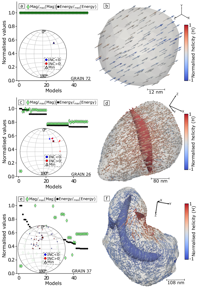
Figure 3: Examples of different types of domain states (for magnetite) and their behaviours are presented here. On the left side, we have compiled the magnetisation (green diamonds) and the corresponding magnetic energy (black dots) for each of the 50 LEM models of a specific grain. These values are normalised by the respective maximum values (of either magnetisation/energy) among the fifty models. The stereographic projections within the plots display the direction of the magnetisation for all models by converting the magnetisation components in the X ($\text{M}_{\text{x}}$), Y ($\text{M}_{\text{y}}$), and Z ($\text{M}_{\text{z}}$) directions to declination $(\text{DEC}=\arctan(M_{y}/M_{x}))$ and inclination $(\text{INC}=\arctan(M_{z}/\sqrt{M_{x}^{2}+M_{y}^{2}}))$. The inclination is coloured according to its polarity (red for positive and blue for negative), and the triangle indicates the direction of the LEM state with the lowest energy (Min). On the right, the minimum free energy model of the corresponding grain is depicted, where the arrows indicate the direction of the magnetisation, and the vortex structures inside are the isosurface hued by the helicity. SD grains show (a,b) practically no difference between the models, whereas SV can exhibit a variety of possible domain states (c,d) with distinct magnetisation (and associated energies), especially when the morphology of the grain is highly irregular (e,f).

The normalised magnetisation of magnetic particles has important implications for the identification of a given domain stature through bulk magnetic properties [15], particularly for non-uniformly magnetised grains, which likely dominate the assembly of stable magnetic carriers in rocks [11]. When we examine the range of a grain’s LEM magnetisation that can be nucleated in each grain, our results indicate that most grains have $\text{Mr}<0.5$, where SV structures are dominant. None of the lowest energy states observed in the LEM models of grains with multi-vortex structures, whether composed of magnetite or maghemite, show a Mr exceeding $0.5$. Remanences greater than such threshold for MV particles have only been observed for higher energy states, which are less stable, while $\text{Mr}>0.5$ (as in Supplementary File, Figure S2a) are essentially displayed by either SD or SV-like structures.

The temporal stability of each grain was determined using the Nudged–Elastic-Band (NEB) method [12]. This allows us to determine the minimum energy path (MEP) between any two given domain states. For each grain, we took the lowest energy state (from a set of 50 random LEM states) and calculated the minimum energy path to its anti-parallel state. In the case where a significant new minimum was observed along the MEP, we subdivided the path at the new intermediate minimum and searched the grain for a new MEP. In this way, we obtained the energy barriers only for the lowest energy LEM state. In this study, we have chosen not to investigate the stability of higher energy (and thus less abundant) states we encountered. The energy barriers from the MEP were converted into magnetisation relaxation times $(\tau)$ using the Néel Arrhenius (Equation 9).

In Figure 4 we show a spectrum of energy barriers, where the vast majority of grains yield relaxation times that far surpass the age of the Solar System. The "eternal" stability includes SD, SV and MV states, the latter having the highest energy barriers. However, four grains have small $\tau$ values. Grain 32 ($\epsilon=0.78,\ \text{P}_{1}=122\ \text{nm},\ \text{P}_{1}/\text{P}_{3}=1.27$), for example, yields a single vortex configuration (Figure 4), but our simulation indicates that thermal energy would overcome magnetic energy in $\tau\approx 3\ \text{hours}$. The other three grains are also elongated but of grain sizes close to our tomography pixel size (e.g., Grain 113, $\epsilon=-0.35,\ \text{P}_{1}=49\ \text{nm},\ \text{P}_{1}/\text{P}_{3}=1.21$). Their relaxation times are mostly instantaneous (Figure 4), which points out that not only size but morphology, is critical in determining domain stability for such small grain sizes.

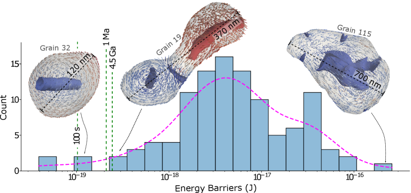
Figure 4: Compilation of the computed magnetic energy barriers for each of the lowest energy LEM states across a minimum energy path to its anti-parallel state, using the Nudged–Elastic-Band (NEB) method [12]. This energy barrier is then applied to the Néel–Arrhenius [8] equation to calculate the relaxation time (at 20 ${}^{\circ}C$) for the transition $\tau$ from one domain state to another. The magenta curve represents the density of the state’s distribution. The vertical dashed lines correspond to $\tau$ for $100$ seconds, $1$ million years, and $4.5$ billion years. Most of the states exhibit stabilities that far surpass the age of the Solar System (as seen in the MV states for Grains 19 and 115). However, a minority of them, such as Grain 32, are unstable magnetic recorders, representing the magnetically unstable zone (MUZ) between the transition of the SD to the ESV state. The colours shown for the arrows within the grains (as well as the vortex structures) have the same meaning as the examples shown in Figure 3 (see colour bar for helicity). Calculations were performed assuming magnetite as the mineral phase.

As stated, when a particle assumes a multiplicity of possible domain states, the issue regarding which of the LEM states is the more likely to be assumed can be resolved in the presence of an isolated energy minimum, as observed in Figure 3c,e. However, some grains may exhibit a more complex behaviour, where the LEM states yield distinct Mr but similar energies. Boltzmann probability distribution of states (Equation 8), shows that for a small number of states at a given temperature, even a small difference of $2\%$ in magnetic energy (e.g., Grain 25 in Supplementary File, Figure S3) between the lowest energy LEM state and other states will result in a $\gg 99.99\%$ occupancy rate of lowest energy state. However, the prevalence of a given state is sometimes also a function of temperature, with the most favoured domain state changing on heating or cooling. We discuss below the case of SV/SD grains with LEM states of similar energies and distinct magnetisations. We intend to investigate how the magnetic energy of these states evolves with an increase in thermal energy, up to the Curie temperature of magnetite. Our observations indicate that the balance between magnetic and thermal energy will also depend upon both the grains’ size and morphology. The SV behaviour can be classified into three groups. The first corresponds to the well-behaved type of grain, where one domain state will prevail up to the Curie temperature (Supplementary File, Figure S3). An example is Grain 25 ($\epsilon=0.43,\ \text{P}_{1}=270\ \text{nm},\ \text{P}_{1}/\text{P}_{3}=3.03$), where $p_{i}$ indicates that a flowering state (of higher magnetisation and lower energy) will prevail over the other competing SV states. The second group represents grains where the energy of one state dominates at lower temperatures, but the magnetic energy becomes similar to other LEM states as the temperature increases (Figure 5a,b). For Grain 68 ($\epsilon=0.60,\ \text{P}_{1}=124\ \text{nm},\ \text{P}_{1}/\text{P}_{3}=1.53$), e.g., a single vortex state (Figure 5b’) dominates until $450\ ^{\circ}\text{C}$ but thereafter $p_{i}$ becomes equally distributed between the other domain states, indicating that any of these states with distinct Mr could be assumed. Finally, the third group behaves poorly. In these grains, the magnetic energies of different domain states are almost indistinguishable with increasing temperature (Figure 5c,d). For grain 48 ($\epsilon=0.07,\ \text{P}_{1}=91\ \text{nm},\ \text{P}_{1}/\text{P}_{3}=1.17$), up to $\sim 300\ ^{\circ}\text{C}$ there is a frequent redistribution of domain states (Figure 5d’), and for T above $300\ ^{\circ}\text{C}$ $p_{i}$ is equally occupied by the three different states.

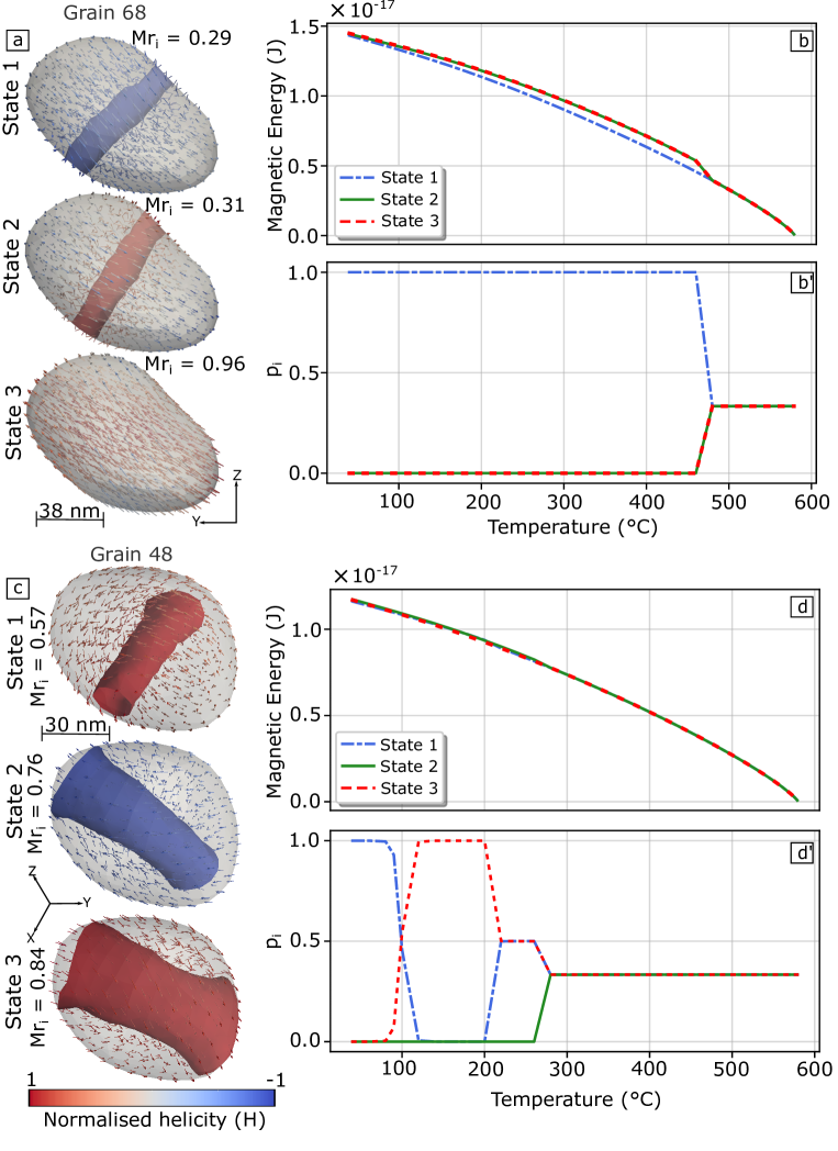
Figure 5: Multiplicity of domain states for grains of magnetite. States with similar energies but distinct magnitudes of magnetisation and their temperature dependence are explored. In the first example (a), States 2 and 3 exhibit slightly higher energy with a temperature increase (b). The Boltzmann probability ($p_{i}$, Equation 8) demonstrates that State 1 will prevail over most of the evaluated temperature range (b’). However, after reaching a certain temperature threshold (approximately $450\ ^{\circ}\text{C}$), the probabilities of these domain states to occur become equal. In the example in (c), this effect is more problematic, as the energies of the states remain practically the same throughout the entire range of temperatures (d), leading to swapping of probabilities between the states (d’) up to nearly $300\ ^{\circ}\text{C}$, from which the $p_{i}$ becomes equally distributed.

Magnetic field-dependent simulations

We have also modelled the hysteresis loops and backfield curves for each of the studied grains (see Methods), accounting for shape anisotropy effects by running models in different field directions and averaging their results. In terms of normalisation, the LEM grain’s magnetisation (Mr) differs from those obtained from the saturation of remanence (Mrs) (see Figures 6, 7). Both of these represent the remanence at zero-field. However, Mrs is determined from the interception of the averaged hysteresis loop, while the Mr is obtained through an energy minimisation starting from a random initial guess. An important effect of averaging over distinct field directions is that saturation (i.e. complete alignment of the magnetisation in the direction of the applied field) at a given field strength will strongly depend on the field direction with respect to the magnetic anisotropy axes of the grain. A particle’s anisotropy is often controlled by its morphology, which then determines how easily a grain becomes magnetically saturated. Therefore, we consider the saturation parameter of magnetic hysteresis, Ms, as the corresponding value of magnetisation for each averaged curve at $250\ \text{mT}$. We apply boxplot statistics to discuss some of the magnetic properties in terms of all grains. As also highlighted in the previous subsection, magnetite and maghemite properties are very similar producing practically indistinguishable results (Figure 6). To avoid redundancies, we henceforth discuss only the properties of magnetite.

Except for a few outliers, the Ms is practically the same as the theoretical one for magnetite ($0.99\pm 0.01$). Mrs span from $0.0035-0.70$, whereas only SD and SV states occupy values greater than $0.5$. Significant discrepancies emerge when comparing Mr with Mrs. Firstly, there is an important influence of the field direction in the whole averaged loop, which can generate very different curves with distinct Mrs for each field direction (Figure 7a,c). For grains whose minimum energy models yield $\text{Mr}\gtrapprox 0.5$, the resulting Mrs from the simulated random distribution of grains can be 50% smaller (Supplementary File, Figure S4a,b). The difference is even greater for particles whose $\text{Mr}\lessapprox 0.5$, which can result in Mrs up to $80\%$ smaller than the magnetisation of its lowest LEM (Mr) (Figure 7). This effect increases with grain size, the larger grains being able to accommodate a larger number of domain states each with a distinct remanence, but this effect is consequently averaged during the field-dependent magnetic experiments or numerical simulations of random distributions of such grains. Bulk coercivities (Bc) span over a large interval ($0.64-80.59\ \text{mT}$, Figure 6), most of them within expected [1] values for magnetite ($11.41\pm 11.86\ \text{mT}$). The coercivity of remanence (Bcr) obtained from the backfield curves is also within the expected range ($46.27\pm 25.32\ \text{mT}$), but several grains present higher values (e.g., Figure 7b), some of these being greater than $100\ \text{mT}$.

The remanence (Mrs/Ms) and the coercivity (Bcr/Bc) ratios are important indicators of magnetic domain states [40]. In Figure 8, we further explore these ratios by making use of the bilogarithmic Day plot (Bcr/Bc vs Mrs/Ms) [41, 40], as well as the Néel’s diagram (Mrs/Ms vs Bc) [8] and its sister plot (Mrs/Ms vs Bcr). The Day plot carries markings of conventional divisions [41, 40] for SD ($\text{Mrs/Ms}\geq 0.5,\ \text{Bcr/Bc}\leq 2$), PSD ($0.5>\text{Mrs/Ms}>2x10^{-2},\ 5>\text{Bcr/Bc}>2$) and MD ($\text{Mrs/Ms}>2x10^{-2},\ \text{Bcr/Bc}>5$) states (Figure 8a). These limits, as well as the interpretation of such parameters, have been questioned [42, 11] to be non-representative of the many processes that can lead to variations of such ratios. Regardless, we keep those fields simply as guides to the eye. On the Day plot, there are two well-defined clusters: for the first one, SD grains and some SV grains group near $\text{Mrs/Ms}=0.5$; for the second one, grains follow a linear trend, $\text{y}=(-0.765\cdot x)-0.682,\ \text{R}^{2}=0.93$. The smallest grains ($100\ \text{nm}\leq$) are within the first cluster (Figure 8a). The grains aligned along the linear trend, which includes both SV and MV states, extend from the original PSD down to the MD region. Besides such an obvious mismatch with the traditional PSD field, some SV states exhibit extremely high Bcr/Bc ratios (Figure 8a), especially associated with larger grains. When all of the backfield and hysteresis are averaged together, our sample produces averaged ratios of $\text{Mrs/Ms}=0.117$ and $\text{Bcr/Bc}=2.45$, which falls within the original PSD field of the Day plot (Figure 8a).

On Néel’s diagram (Figure 8b), the same clusters are also present, which is expected since they share the same ordinate axis. Bc of the first cluster has a quite spread behaviour, but the other grains show a linear increase of remanence with the bulk coercivity, $\text{y}=(1.215\cdot x)-2.282,\ \text{R}^{2}=0.91$. This relationship is inversely proportional to the coercivity of remanence (Figure 8c) for which, although more dispersed, Bcr increases as the remanence ratio decreases, $\text{y}=(-1.212\cdot x)+0.619,\ \text{R}^{2}=0.56$. For all the properties here discussed, there is no clear relationship between a magnetic property and the respective elongation parameter of a grain. However, even for these irregularly shaped grains, there seems to be a correlation between the magnitude of Bcr and the grain size. When we put together experimental data [41, 43, 44, 45, 46, 47, 48, 49, 50, 51, 52, 53] and the results of our models, despite a large spreading, the coercivity of remanence seems to increase and peak around grain sizes between $600-700\ \text{nm}$, from which it tends to decay again (Figure 8d).

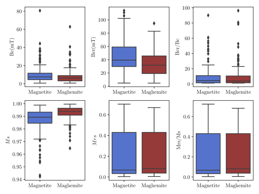
Figure 6: A compilation of parameters obtained from the magnetic hysteresis loops and backfield curves for magnetite (blue) and maghemite (brown) is presented using boxplot statistics. These parameters correspond to averaged curves obtained for each grain in twenty different directions (refer to Methods for details). Bc represents the bulk coercivity, Bcr is the coercivity of remanence, Ms indicates the magnetisation saturation of the averaged loop at the maximum field, and Mrs is the remanence of saturation. Black diamonds signify statistical outliers. As illustrated, magnetite and maghemite exhibit practically indistinguishable properties.

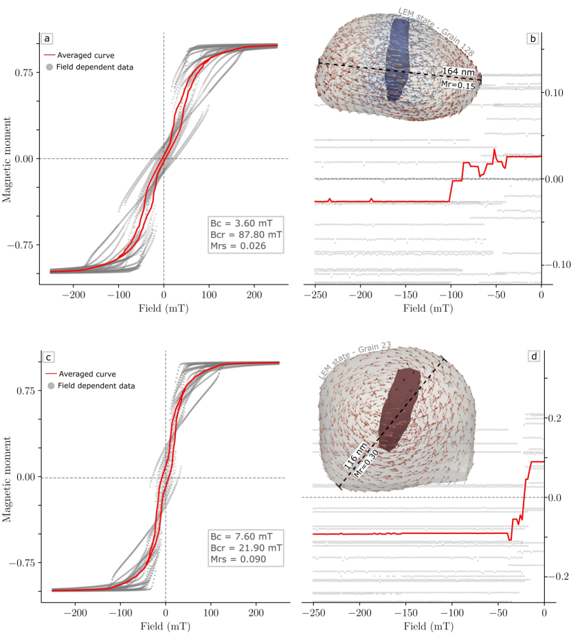
Figure 7: Examples of magnetic hysteresis (a, c), backfield curves (b, d), and their parameters (for magnetite). The grey dots represent the field-dependent data, and the red curves depict their averages. Notably, for both types of simulated experiments, different field directions result in distinct curves as a result of the grain’s shape anisotropy. The particles situated at the upper side of the backfield curves (b, d) correspond to the LEM states obtained at zero field. Here, we highlight how the Mr of these states might differ significantly from the Mrs of magnetic hysteresis (compare the Mrs values within the boxes in a and c with the respective Mr values within the grains).

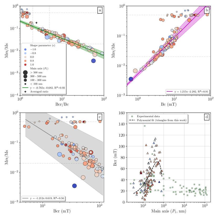
Figure 8: a) Remanence (Mrs/Ms) and coercivity (Bcr/Bc) ratios are compared in the Bilogarithmic Day plot [41, 40]. Two distinct clusters are evident: the first, located near $\text{Mrs/Ms}\approx 0.5$, and the second, following a linear trend (green line with shaded extension representing $\alpha 95$). For a, b and c, the circles are colour-coded based on the shape parameter ($\epsilon$), with blue/red indicating more prolate/oblate grains. The circle size represents grain size, and the black cross (in a) indicates the average ratio of all modelled grains. Neél’s diagram [8] (b) and its sister plot (c) depict linear tendencies with confidence areas. Similar clusters are observed in both plots, indicating an increase in remanence with coercivity (Bc) and a decrease with the increase of coercivity of remanence (Bcr). In plot d, Bcr values obtained in our models (triangles) are compared with their respective grain sizes, while green squares represent experimental data [41, 43, 44, 45, 46, 47, 48, 49, 50, 51, 52, 53]. A third-order polynomial fit serves as a guide, revealing a trend where Bcr peaks around $600-700nm$ before decreasing, consistent with experimental findings.

Discussion

On the magnetic properties of natural nanoscopic grains

Although not surprising, an important aspect of our results is that the magnetic properties of magnetite and maghemite, as demonstrated in Figure 6, as well as their domain states, are practically indistinguishable at ambient temperatures. The challenge of differentiating between these two magnetically soft minerals can be addressed through the use of temperature-dependent experiments [1], which are proven to be essential for properly interpreting environmental magnetism data and inferring exogenous processes [54], but often expose the samples to chemical or domain state change.

Mrs/Ms and Bcr/Bc ratios derived from magnetic hysteresis and backfield curves can be characteristic for an entire assemblage of grains. It is natural, therefore, that various processes impact the comparison of these ratios in the Day plot [41, 40]. Such processes include mixtures of magnetic minerals with distinct coercivities, and/or mixtures of grains in distinct domain states [55, 56], as well as surface oxidation, mineral stoichiometry, and the intrinsic magnetic properties of each grain [42]. Nevertheless, our data demonstrates that for both magnetite and maghemite (Figure 8a), two well-defined clusters exist. One is occupied by higher remanences (solely featuring SD and SV states), and the other displays a linear trend cutting across the Day plot towards lower remanence ratios and higher coercivity ratios. The Day plot trend we observe for SV grains closely follows that found in idealised grains by Williams et al [57], although, for our irregular grains, we do not observe a well-defined correlation with grain shape. As grain sizes increase, so does the internal demagnetising field [9, 15], until it grows sufficiently strong to collapse into a lower energy domain state. Lower energy domain states often imply a decrease in remanence, which we observe in our analysis with the increase in Bcr (Figure 8b). Our data also suggests a peak for Bcr with the increase of grain size around $600-700\ \text{nm}$ (Figure 8d), aligning considerably with experimental data of grains with distinct morphologies and sizes [41, 43, 44, 45, 46, 47, 48, 49, 50, 51, 52, 53]. Generally, our results also align well with data derived from iron oxide inclusions [22].

In our simulations, the influence of superparamagnetic (SP) grains is not resolved. The combination of all grains in hysteresis and backfield curves suggests that a high quantity of SP particles could potentially decrease Mrs/Ms and increase Bcr/Bc [40]. Careful interpretation of these diagrams is necessary. However, with well-established magnetic mineralogy supported by other analyses such as thermal demagnetisation of synthetic remanences, thermomagnetic curves, first-order reversal curves (FORCs), and chemical/imaging analyses, the Day plot, Néel’s diagram, and related plots can provide useful insights.

Magnetic hysteresis, including FORCs[58, 59, 60], heavily rely on the Mrs to infer field-induced states and not remanence states. One of our crucial observations is that unless the grains are SD, the true remanence of a grain will be potentially underestimated. While this may not be a significant concern for very fine particles exhibiting SD-like behaviour ($\text{Mrs}\gtrapprox 0.5$), it can become a pronounced phenomenon for larger grain sizes. Experimentally, magnetic hysteresis, backfield curves, isothermal remanence curves (IRMs), and FORCs are performed using a fixed field direction. As illustrated in Figure 7, the applied field’s direction can induce variable magnetic properties due to the grains’ shape anisotropy. For a population of irregular grains randomly oriented, changing the field direction may not significantly decrease this effect because rocks might have millions of magnetic grains. However, for materials with a well-oriented magnetic fabric (e.g., inclusions in minerals, and highly deformed rocks), conducting these measurements in variable field directions (or changing sample orientation) might enhance the determination of Mrs.

Temporal and thermal stability of irregularly shaped grains

The capacity of magnetic minerals to retain their remanence over geological time-scales is crucial for planetary studies, as rock-magnetic recordings provide information on Earth and Planetary evolution such as tectonics [2], the timing of inner core nucleation [61], and even the early stages of solar nebula development [62]. Néel’s theory [8] has long been employed to demonstrate that SD grains can retain their remanence over billions of years. Although this domain state is highly stable, it spans only a very limited range of sizes, and most terrestrial and extraterrestrial magnetic materials will contain a much broader range of grain sizes.

Nagy et al. [12] have calculated the temporal stability of equidimensional truncated octahedron grains of magnetite ($80-1000\ \text{nm}$) in the SV state and have demonstrated that, except for grains between $80-100\ \text{nm}$, their stability surpasses the age of the Solar System. Our calculations for non-euhedral morphologies, which are more realistic for oxide grains in most natural systems, generally align with this interpretation (Figure 4), demonstrating that most SV and MV grains can also retain eternal stability at environmental temperatures. Nagy et al. [12] also pointed to a magnetically unstable zone (MUZ) for grain sizes between $80-100\ \text{nm}$, for which the relaxation times are near instantaneous at room temperature. In the MUZ for magnetite, the SV domain state is aligned with the hard magnetisation axis (HSV), while large SV grains align their magnetisation with the easy magnetic anisotropy axis (ESV). Wang et al. [13], have shown that within the MUZ ($68-100\ \text{nm}$) the grains’ evolution proceeds as SD $\rightarrow$ HSV $\rightarrow$ ESV. For such, grains within the MUZ were shown to occupy about $20\ \text{nm}$ for euhedral and also for rounded particles [18, 63]. Four of our modelled grains within the MUZ size range proposed by Nagy et al. [12] are unstable at room temperature, e.g. Grain 32 (Figure 4) with an elongation axis of $122\ \text{nm}$. Furthermore, several of the grains (with variable morphology) that we studied have $\text{P}_{1}$ within the proposed range dimensions of the MUZ (e.g., Grain 135: $\epsilon=-0.93,\ \text{P}_{1}=80\ \text{nm},\ \text{P}_{1}/\text{P}_{3}=1.39$ | Grain 48: $\epsilon=0.07,\ \text{P}_{1}=91\ \text{nm},\ \text{P}_{1}/\text{P}_{3}=1.17$), and yet they are highly stable. Therefore, we suggest that the transition of SD to HSV (consequently at the onset of the MUZ) is strongly affected by the morphology of the grain.

Figure 3 further highlights that a multiplicity of domain states may occur in one or more temperature intervals and that the likelihood of a grain being able to nucleate multiple domain states increases with grain size. This is a particular problem for the determination of palaeointensities which are often performed using a stepwise cycle of heating, where the original remanence (a thermal remanence, TRM) in any temperature interval is replaced by laboratory-induced partial thermal remanence (pTRM) in a known field. [64, 65]. An important assumption in these experiments is that the magnetic recorders in the sample obey the so-called Law of Reciprocity, which states that a magnetic grain demagnetises (unblocks) and re-magnetises (blocks) at the same temperature i.e. ($T_{ub}=T_{b}$) [66, 64, 67], which is only valid for the original SD theory of Néel. When multiple domain states are possible in the same grain, thermal cycling may produce a pTRM with grains now occupying very different domain states with different thermal stabilities, such that $T_{ub}\neq T_{b}$. This issue has been discussed by Nagy et al. [14]. In their models, using a euhedral magnetite grain ($100\ \text{nm}$, with $30\%$ of elongation along [$100$]), they not only point to a multiplicity of domain states but also to a preference for a given state as temperature changes, especially as a function of the cooling ratio. A similar effect has been identified by Tauxe [67] where "fragile" magnetic remanences behaved differently during stepwise demagnetisation and remagnetisation after samples "aged" by sitting in various storage fields over many months. This time-induced effect is equivalent to the pure thermal effect described by Nagy et al. [14], which would be caused by the multiplicity of possible domain states.

We now suggest this situation might affect a much broader range of grain sizes, and be highly dependent on grain morphology. Any failure of blocking and unblocking reciprocity, as well as the often large change in a grain’s magnetisation, will make it impossible to obtain reliable paleomagnetic intensities. In exploring the multiplicity of domain states that co-exist with similar magnetic free energies for grains of irregular shape we observed this same problem. Grains whose behaviour is dominated by one or two states over a large range of temperatures are the ones that will likely provide good paleointensity results up to a certain temperature, where the difference in energy is significant. Above such temperature threshold, any of the possible domain states could be assumed as the probability is equally distributed (Figure 5b’). The exact occupancy of the different domain states will be dependent on the thermomagnetic history of the sample. Repetitive cycling through temperatures, each yielding a variety of domain states, is expected to gradually shift the overall distribution of domain states within the sample, deviating from the initial distribution that carried the original (geological) recording of the geomagnetic field. Thus, thermal cycling and differential heat/cool rates are likely to further exacerbate the problem [14]. It is possible that grains exhibiting the two dominant state behaviours (Figure 5b’) could in some instances be an alternative explanation to high temperature palaeomagnetic experimental failure that is often attributed to chemical alteration [68]. Grains with more complex behaviour (Figure 5d’), characterised by a constant re-balancing of probabilities, are expected to yield unreliable thermally dependent paleomagnetic and paleointensity data, similar to the findings presented by Nagy et al. [14].

Magnetic grains whose domain states are either truly SD or ESV but far from such transition zones (mostly grains $\gtrapprox 200\ \text{nm}$) are likely to be the most stable magnetic recorders, and also the ones for which palaeomagnetic information is less affected by thermal experiments. That is probably because the mechanism for magnetic state transitioning of ESV grains is the structure coherent rotation [12], which (as well as for SD grains) requires a uniform rotation of all of the magnetic moments associated with the grain. Furthermore, because domain state transitions seem to imply several complications in the magnetic properties of grains, there should be an equal dedication to studying grains within the ESV $\rightarrow$ MV transition.

Methods

Sample preparation

The sample used in our research is a Neoproterozoic cap carbonate rock, part of the Guia Formation, which spreads over the Amazon craton and the Paraguay belt (central-West Brazil). These rocks have been targets of palaeomagnetic studies and suggested to carry pervasive evidence of authigenic growth of secondary magnetic grains as a result of low-temperature (<Tc) chemical processes [30, 69]. Recently, Bellon et al. [29] performed a mineralogical, microscopic and magnetic analysis on remagnetized carbonate rocks from South America. We have chosen a thin-section sample from their data set that has shown remarkable amounts of micrometric/nanometric iron oxides to build continuous work. Preparation of microscopic pillars was acquired by firstly coating the thin sections with carbon and sequentially cutting a $\approx 18\times 40\mu\text{m}$ pillar using a FIBSEM Helios 600i TFS FIB-SEM (Scientific Center for Optical and Electron Microscopy - ScopeM, EHT Zürich). Because the pillar sample represents only an infinitesimal part of the macroscopic thin section, the pillar was prepared in a region that had been chemically mapped for iron oxides through both SEM-EDS and synchrotron-based X-ray Fluorescence/X-ray Absorption Near Edge Spectroscopy (XRF/XANES), [29]. Lastly, the pillar was mounted on a PXCT OMNY-pin [28] using a nanomanipulator.

Synchrotron-based Ptychographic X-ray Computed Nano-tomography (PXCT)

PXCT was performed at the cSAXS (coherent small-angle X-ray scattering) beamline of the Swiss Light Source at the Paul Scherrer Institute (PSI, Villigen, Switzerland). For the acquisition, we used the flOMNI setup [70, 26], a photon energy of 6.2 keV, and we placed the sample downstream of the focal spot defined by a Fresnel zone plate (FZP). This energy was chosen due to the major mineral constituent being calcite $(\text{CaCO}_{3})$, which results in nearly $50\%$ of transmission in the middle of the sample for a pillar of 20 $\mu$m. Scans were performed in a Fermat spiral pattern[71] with a field of view of $37\times 10\,\mu\text{m}$, and coherent diffraction patterns were collected with an Eiger $1.5\text{M}$ detector [72] positioned $5.229\text{m}$ downstream of the sample. We acquired $650$ projections at different incidence angles of the beam from the sample, ranging from $0$ to $180^{\circ}$. During the data collection, we estimate that a dose of $5.6\times 10^{8}\ \text{Gy}$ was delivered to the sample. Reconstruction of ptychographic projections were performed with the PtychoShelves package developed by the Coherent X-ray Scattering group at PSI [73], using a combination of the difference map algorithm [74], followed by the maximum likelihood algorithm [75]. This resulted in images with a pixel size of $34.8\ \text{nm}$. Phase images were treated with the removal of offset and linear terms and were further aligned in the vertical and horizontal directions with a subpixel precision method [76, 77]. Tomographic reconstructions were finally performed by applying a filtered back projection [76, 77]. Using Fourier shell correlation (FSC) [78], we estimated that the average 3D half-pitch resolution of the whole 3D dataset is $89\text{nm}$. This resolution reflects the specimen’s overall average. The limited quantity of high-density magnetite particles could be imaged with better resolution due to their contrasting density with the surrounding material. More details about the PXCT experimental setup, data collection and reconstruction can be found in the Supplementary File.

Segmentation and processing of tomographic data

Distinguishing from traditional X-ray microscopy techniques, X-ray ptychography provides images of the complex-valued transmissitivity of the specimen, where the real part is related to the absorption and the imaginary part with the phase shift of the X-rays. In combination with tomography, PXCT provides the 3D distribution of the full complex index of refraction $n(\vec{r})$ [23]:

$$n(\vec{r})=1-\delta(\vec{r})-i\cdot\beta(\vec{r})$$ (1)

where $\delta(\vec{r})$ and $\beta(\vec{r})$ are obtained from the tomographic reconstruction using the phase and the absorption images, respectively. The phase shift of X-rays is related to refraction, which describes the change in the direction of the X-rays, it is strongly associated with the material density, composition and internal structure, while absorption of X-rays is related to the local structure and composition environment of an adsorbing atom, apart from its density. In our paper, we rely on the $\delta(\vec{r})$ reconstructed tomography to recover the morphology and segment different mineral constituents of the pillar due to its higher resolution compared to the $\beta(\vec{r})$ tomogram. Nevertheless, we compare that data with $\beta(\vec{r})$ reconstruction to refine our interpretation. The quantitative $\delta(\vec{r})$ values obtained at each voxel are converted to electron density $n_{e}(\vec{r})$ as [79]:

$$n_{e}(\vec{r})=\frac{\delta(\vec{r})k^{2}}{r_{0}2\pi}$$ (2)

where $k=(2\pi/\lambda)$, $\lambda$ is the X-ray wavelength and $r_{0}$ is the Thomson scattering length. In order to compare with our data, we can use the theoretical relation between the mass density of a given material $\rho(\vec{r})$ and its $n_{e}(\vec{r})$ as [80]:

$$\rho(\vec{r})=\frac{n_{e}(\vec{r})\cdot A}{N_{A}\cdot\phi}$$ (3)

where A is the molar mass, $N_{A}$ is Avogadro’s number and $\phi$ is the total number of electrons in a molecule of the material.

After converting the $\delta$ values to electron density (Equation 2), we calculated the histogram distribution of all voxels in the tomogram to segment the distinct populations composing the sample (Supplementary File, Figure S1c). Before segmenting the data, we first deal with salt-and-pepper noise (maximum/minimum intensity voxels randomly distributed throughout the image [81]) by applying a three-dimensional Gaussian filter to the data (assuming an isotropic $\sigma=1$, centred at each voxel). Data segmentation was acquired by processing the natural breaks in the histogram distribution and using them as thresholds after stripping away the air response. Based on the $n_{e}$ distribution, five classes have been defined (Supplementary File, Figure S1d). The $n_{e}$ slices were reclassified into binary files, assigning True for the iron oxides and False for all of the other materials. Binary files were then imported to the software Dragonfly to generate stereolithographic data (STL file) of each iron oxide grain. Even aware that filtering would be able to deal with salt-and-pepper noise, we have removed particles represented by a single voxel, to give more robustness to our models.

To systematically acquire information on the morphology of the iron oxides we used a Principal Component Analysis (PCA) of their spatial distribution. Firstly, we export the STL files as a Cartesian coordinate cloud of points (x, y, and z) describing the external morphology of the particle. Sequentially, we use a Python script to calculate the convex hull [82] of each set of coordinates of a given particle. A convex hull is the smallest possible convex shape that encloses a given set of points, forming a polygon that connects the outermost points by ensuring that all of its internal angles are less than 180^∘ [83]. We then performed a PCA [84], to get the eigenvectors (main directions) and eigenvalues (their magnitudes) of a covariance matrix of standardised variables. Sequentially, we have projected the original convex hull vertices onto the space defined by the principal components and calculated the size of the hull along the main directions. In this case, the maximum variance component $\text{P}_{1}$ represents the maximum elongation axis, $\text{P}_{2}$ is the intermediary one and $\text{P}_{3}$ is the minimum variance component (short axis). To more broadly evaluate the morphology of the particles in our sample, we use the shape parameter (here called $\epsilon$) of Nikolaisen et al. [22] by using our main components achieved through the PCA analysis:

$$\epsilon=\log\left(\frac{\text{P}_{1}-\text{P}_{2}}{\text{P}_{2}-\text{P}_{3}}\right)$$ (4)

for which triaxial morphologies (all of the main axes have different dimensions) will have $\epsilon\approx 0$, the more positive $(\epsilon>>0)$ more oblate is the grain, and the more negative $(\epsilon<<0)$ more prolate is the grain.

Micromagnetic modelling

Finite element meshes and magnetic properties

In micromagnetic models, physical processes and their respective energies are evaluated mathematically through a continuous function, by assuming that at a given spatial volume the magnetisation is an average of discrete physical sources of magnetism, and that such volume is representative of the individual atomic behaviour of the averaged atoms [85, 86, 10]. To solve the local energy minimum (LEM) for each of the iron oxides identified in our tomography, we rely on the open-sourced software package MERRILL [10]. This software uses linear tetrahedral finite elements to describe the geometry of a particle and solve the LEM stable states minimising the free energy of a magnetic system $E=\vec{H}_{\text{eff}}\cdot\vec{M}$, for which the total effective field $(\vec{H}_{\text{eff}})$ is [10]:

$$\vec{H}_{\text{eff}}(\vec{M)}=\vec{H}_{\text{exg}}(\vec{M)}+\vec{H}_{\text{ans}}(\vec{M)}+\vec{H}_{\text{Zmn}}(\vec{M)}+\vec{H}_{\text{dmg}}(\vec{M)}$$ (5)

where $\vec{M}$ is the magnetisation vector, $\vec{H}_{\text{exg}}$ the exchange field, $\vec{H}_{\text{ans}}$ the anisotropy field, $\vec{H}_{\text{Zmn}}$ the Zeeman field, and $\vec{H}_{\text{dmg}}$ is the demagnetising field. We have used the software Cubit to build the tetrahedral meshes of each particle (previously exported as a STL file). To ensure that our finite element meshes were fine enough to resolve the spatial variation of the magnetisation within the geometry of each grain we determined the maximum element size as dependent on their exchange length $\text{I}_{\text{e}}$ [38]. $\text{I}_{\text{e}}$ of magnetite $(\text{Fe}_{3}\text{O}_{4})$ is $\approx 9\ \text{nm}$ at environmental conditions of temperature and pressure, and slightly larger than that near its Tc [10]. The exchange length of maghemite $(\gamma\text{Fe}_{2}\text{O}_{3})$ is slightly larger than magnetite’s, so it is not an issue to assume $9\ \text{nm}$ as a maximum element size for both mineralogies. Magnetic parameters of these minerals are set as in Table 1.

Table 1: Magnetic properties of the iron oxides used in our micromagnetic models at $20\ ^{\circ}\text{C}$. $A_{ex}$ is the exchange constant, $K_{1}$ is the anisotropy constant, and $M_{s}$ is the magnetisation saturation.

Mineral	Anisotropy	$A_{ex}$	$K_{1}$	$M_{s}$	Ref
Magnetite $(Fe_{3}O_{4})$	Cubic	$1.33\cdot 10^{-11}$	$-1.24\cdot 10^{4}$	$4.8\cdot 10^{5}$	Heider and Williams [87]
Maghemite $(\gamma Fe_{2}O_{3})$	Cubic	$1\cdot 10^{-11}$	$-4.6\cdot 10^{3}$	$3.8\cdot 10^{5}$	Dunlop and Özdemir [15]

Numerical calculations

For any micromagnetic experiment performed through MERRILL, we can achieve a visualisation of the magnetic energy within the particles by performing simple mathematical operations to better illustrate the finite element solutions. We have achieved that through the open-sourced software Paraview [88]. Firstly, we calculate the curl of the magnetisation $\vec{M}=M_{x}\hat{i}+M_{y}\hat{j}+M_{z}\hat{k}$, which is basically its vorticity $(\vec{\omega})$, as:

$$\vec{\omega}=\nabla\times\vec{M}$$ (6)

Sequentially, we calculate the projection of $\vec{\omega}$ onto $\vec{M}$, which is the normalised helicity $(\vec{H})$ shown in our figures, as:

$$\vec{H}=\frac{\vec{M}\cdot\vec{\omega}}{\lVert\vec{\omega}\rVert}$$ (7)

When starting from random initial orientations, LEM calculations might reach slightly different products resulting from local minima. We calculate fifty (50) different LEM models for every grain at $20\ ^{\circ}\text{C}$ and then harvest the states with the lowest minimised energies to reach the most stable magnetic domains (here called $r$). Upon categorising the states by their energies and magnetisation intensity/direction, we can determine the probability ($p_{i}$) associated with a particular state. This probability is expressed as a function of the state’s energy and the system temperature, in the presence of other states, utilising a normalised Boltzmann probability distribution:

$$p_{i}=\frac{\exp\left(-(\varphi_{i}-\lambda_{j})\right)}{\sum_{j}^{r}\exp\left(-(\varphi_{j}-\lambda_{j})\right)}$$ (8)

Here, $\varphi_{i}=\frac{E_{Mi}}{k_{B}\cdot T}$, where $E_{Mi}$ represents the magnetic energy (in J) of the state under consideration; $k_{B}$ is the Boltzmann constant $(1.3806\times 10^{-23}\ \mathrm{m^{2}\cdot kg\cdot s^{-2}\cdot K^{-1}})$; and the temperature of the system, denoted as $T$ (in K). Additionally, $\lambda_{j}$ is defined as $\min(\varphi_{j})$. To ascertain the probability $(p_{i})$ under varying temperatures, we conducted LEM minimisations for selected examples. In this process, each of the $r$-states served as the initial solutions. The temperatures ranged from $40-579\ ^{\circ}\text{C}$, with intervals of $20\ ^{\circ}\text{C}$ up to $500\ ^{\circ}\text{C}$, followed by intervals of $10\ ^{\circ}\text{C}$ up to $570\ ^{\circ}\text{C}$, and finally, $1\ ^{\circ}\text{C}$ increments up to $579\ ^{\circ}\text{C}$.

To assess the temporal stability of magnetic particles at environmental temperatures, we employed the Nudged–Elastic-Band (NEB) method [12]. Initially, we sampled the minimum energy state of a given particle, and inverted the direction of magnetisation, resulting in two opposite (mirrored) domain states. The NEB method was then utilised to determine the magnetic energy (called energy barrier) required for the transition from one domain state to the other. For that, we simply gather the energy difference between the global maximum and minimum of the pathway. Subsequently, we have used this energy to calculate the relaxation time $(\tau)$ for each grain through the Néel–Arrhenius [8] equation as follows:

$$\tau=C\cdot\exp\left(\frac{Em}{k_{B}\cdot T}\right)$$ (9)

where $C=10^{-9}\ \text{s}$ is a frequency factor, and $T$ is fixed at $293.15\ \text{K}$.

Magnetic hysteresis were evaluated from $-250\ \text{mT}$ to $250\ \text{mT}$ in $2\ \text{mT}$ steps, while backfield curves were evaluated from $0$ to $-250\ \text{mT}$ using the same field steps, as this range covers the expected coercivity of such magnetic minerals. In our magnetic hysteresis simulations, we assess the magnetisation of a material under the influence of an applied magnetic field. The process initiates with saturation magnetisation (Ms) in a specific field direction, achieved at the maximum applied field. Subsequently, the field is gradually reduced to zero, resulting in the remanence of saturation (Mrs) at zero field. Following this, a magnetic field in the opposite direction (negative) is induced, where the field eventually causes the magnetisation to be zero (which is the coercivity, Bc), ultimately reaching the saturation point again. Backfield curves follow a similar process with a slight modification. The sample is first saturated, starting at zero field (Mrs). The field is then increased in steps, and before moving to a new step, it is decreased to zero. The remaining remanence is recorded, and as the remanence approaches zero, the coercivity of remanence (Bcr) is determined. To put it simply, magnetic hysteresis involves measuring magnetisation under the influence of a magnetic field, while backfield curves are influenced by a magnetic field, but the field is "turned off" during the actual "measurement" of the magnetisation. In our simulations of magnetic field-dependent experiments, the grain’s shape can create anisotropic properties due to easy/hard magnetisation axes. To account for this, we simulate different magnetic field orientations by sampling a field-dependent magnetic property $F_{i}$ from random 3D coordinates (drawn from a Fibonacci sequence) on a unit sphere as:

$$\iint_{s}{f(x,y,z)}\ ds\ \approx\ \sum_{i=1}^{20}\frac{F_{i}}{20}$$ (10)

Here (Equation 10), $f(x,y,z)$ evaluates the magnetic property $F_{i}$, and the integral over the surface $s$ is approximated by the sum over all samples. Because increasing the number of samples improves the approximation, we have run field-dependent experiments in twenty ($\text{n}=20$) random directions for every grain.

References

- [1] Tauxe, L. Essentials of paleomagnetism (Univ of California Press, 2010).
- [2] Merdith, A. S. et al. Extending full-plate tectonic models into deep time: Linking the neoproterozoic and the phanerozoic. \JournalTitleEarth-Science Reviews 214, 103477, DOI: https://doi.org/10.1016/j.earscirev.2020.103477 (2021).
- [3] Bono, R. K. et al. The PINT database: a definitive compilation of absolute palaeomagnetic intensity determinations since 4 billion years ago. \JournalTitleGeophysical Journal International 229, 522–545, DOI: 10.1093/gji/ggab490 (2021). https://academic.oup.com/gji/article-pdf/229/1/522/42020748/ggab490.pdf.
- [4] Labrosse, S. & Macouin, M. The inner core and the geodynamo. \JournalTitleComptes Rendus Geoscience 335, 37–50, DOI: https://doi.org/10.1016/S1631-0713(03)00013-0 (2003).
- [5] Driscoll, P. E. Simulating 2 ga of geodynamo history. \JournalTitleGeophysical Research Letters 43, 5680–5687, DOI: https://doi.org/10.1002/2016GL068858 (2016).
- [6] Zhou, T. et al. Early Cambrian renewal of the geodynamo and the origin of inner core structure. \JournalTitleNature Communications 13, 4161, DOI: 10.1038/s41467-022-31677-7 (2022).
- [7] Liu, Q. et al. Environmental magnetism: Principles and applications. \JournalTitleReviews of Geophysics 50, DOI: https://doi.org/10.1029/2012RG000393 (2012). https://agupubs.onlinelibrary.wiley.com/doi/pdf/10.1029/2012RG000393.
- [8] Néel, L. Some theoretical aspects of rock-magnetism. \JournalTitleAdvances in Physics 4, 191–243, DOI: 10.1080/00018735500101204 (1955).
- [9] Williams, W. & Dunlop, D. J. Three-dimensional micromagnetic modelling of ferromagnetic domain structure. \JournalTitleNature 337, 634–637, DOI: 10.1038/337634a0 (1989).
- [10] Ó Conbhuí, P. et al. Merrill: Micromagnetic earth related robust interpreted language laboratory. \JournalTitleGeochemistry, Geophysics, Geosystems 19, 1080–1106, DOI: https://doi.org/10.1002/2017GC007279 (2018). https://agupubs.onlinelibrary.wiley.com/doi/pdf/10.1002/2017GC007279.
- [11] Lascu, I., Einsle, J. F., Ball, M. R. & Harrison, R. J. The vortex state in geologic materials: A micromagnetic perspective. \JournalTitleJournal of Geophysical Research: Solid Earth 123, 7285–7304, DOI: https://doi.org/10.1029/2018JB015909 (2018). https://agupubs.onlinelibrary.wiley.com/doi/pdf/10.1029/2018JB015909.
- [12] Nagy, L. et al. Stability of equidimensional pseudo–single-domain magnetite over billion-year timescales. \JournalTitleProceedings of the National Academy of Sciences of the United States of America 114, 10356–10360, DOI: 10.1073/pnas.1708344114 (2017).
- [13] Wang, Y. et al. Micromagnetic modeling of a magnetically unstable zone and its geological significances. \JournalTitleJournal of Geophysical Research: Solid Earth 127, e2022JB024876, DOI: https://doi.org/10.1029/2022JB024876 (2022). E2022JB024876 2022JB024876, https://agupubs.onlinelibrary.wiley.com/doi/pdf/10.1029/2022JB024876.
- [14] Nagy, L., Williams, W., Tauxe, L. & Muxworthy, A. Chasing tails: Insights from micromagnetic modeling for thermomagnetic recording in non-uniform magnetic structures. \JournalTitleGeophysical Research Letters 49, e2022GL101032, DOI: https://doi.org/10.1029/2022GL101032 (2022). E2022GL101032 2022GL101032, https://agupubs.onlinelibrary.wiley.com/doi/pdf/10.1029/2022GL101032.
- [15] Dunlop, J. & Özdemir, O. Rock Magnetism: Fundamentals and frontiers (Cambridge University Press, Cambridge, 1997), 1 edn.
- [16] Schabes, M. E. & Bertram, H. N. Magnetization processes in ferromagnetic cubes. \JournalTitleJournal of Applied Physics 64, 1347–1357, DOI: 10.1063/1.341858 (1988). https://pubs.aip.org/aip/jap/article-pdf/64/3/1347/8003858/1347_1_online.pdf.
- [17] Muxworthy, A. R., Dunlop, D. J. & Williams, W. High-temperature magnetic stability of small magnetite particles. \JournalTitleJournal of Geophysical Research: Solid Earth 108, DOI: https://doi.org/10.1029/2002JB002195 (2003). https://agupubs.onlinelibrary.wiley.com/doi/pdf/10.1029/2002JB002195.
- [18] Nagy, L., Williams, W., Tauxe, L. & Muxworthy, A. R. From nano to micro: Evolution of magnetic domain structures in multidomain magnetite. \JournalTitleGeochemistry, Geophysics, Geosystems 20, 2907–2918, DOI: https://doi.org/10.1029/2019GC008319 (2019). https://agupubs.onlinelibrary.wiley.com/doi/pdf/10.1029/2019GC008319.
- [19] Kopp, R. E. & Kirschvink, J. L. The identification and biogeochemical interpretation of fossil magnetotactic bacteria. \JournalTitleEarth-Science Reviews 86, 42–61, DOI: https://doi.org/10.1016/j.earscirev.2007.08.001 (2008).
- [20] Chang, L. et al. Giant magnetofossils and hyperthermal events. \JournalTitleEarth and Planetary Science Letters 351-352, 258–269, DOI: https://doi.org/10.1016/j.epsl.2012.07.031 (2012).
- [21] de Groot, L. V. et al. Determining individual particle magnetizations in assemblages of micrograins. \JournalTitleGeophysical Research Letters 45, 2995–3000, DOI: https://doi.org/10.1002/2017GL076634 (2018). https://agupubs.onlinelibrary.wiley.com/doi/pdf/10.1002/2017GL076634.
- [22] Nikolaisen, E. S., Harrison, R. J., Fabian, K. & McEnroe, S. A. Hysteresis of natural magnetite ensembles: Micromagnetics of silicate-hosted magnetite inclusions based on focused-ion-beam nanotomography. \JournalTitleGeochemistry, Geophysics, Geosystems 21, e2020GC009389, DOI: https://doi.org/10.1029/2020GC009389 (2020). https://agupubs.onlinelibrary.wiley.com/doi/pdf/10.1029/2020GC009389.
- [23] Dierolf, M. et al. Ptychographic X-ray computed tomography at the nanoscale. \JournalTitleNature 467, DOI: 10.1038/nature09419 (2010).
- [24] Jackson, M. & Swanson-Hysell, N. L. Rock magnetism of remagnetized carbonate rocks: another look. In Remagnetization and Chemical Alteration of Sedimentary Rocks, DOI: 10.1144/SP371.3 (Geological Society of London, 2013).
- [25] Elmore, R. D., Muxworthy, A. R., Aldana, M. M. & Mena, M. Remagnetization and Chemical Alteration of Sedimentary Rocks (Geological Society of London, 2013).
- [26] Holler, M. et al. X-ray ptychographic computed tomography at 16 nm isotropic 3D resolution. \JournalTitleScientific Reports 4, 1–5, DOI: 10.1038/srep03857 (2014).
- [27] Michelson, A. et al. Three-dimensional visualization of nanoparticle lattices and multimaterial frameworks. \JournalTitleScience 376, 203–207 (2022).
- [28] Holler, M. et al. OMNY PIN—A versatile sample holder for tomographic measurements at room and cryogenic temperatures. \JournalTitleReview of Scientific Instruments 88, 113701, DOI: 10.1063/1.4996092 (2017). https://pubs.aip.org/aip/rsi/article-pdf/doi/10.1063/1.4996092/15842226/113701_1_online.pdf.
- [29] Bellon, U. D. et al. Clay minerals and continental-scale remagnetisation: a case study of south american neoproterozoic carbonates. \JournalTitleAuthorea, Inc. DOI: http://dx.doi.org/10.22541/essoar.170365187.73154915/v1 (2023).
- [30] Font, E., Trindade, R. I. F. & Nédélec, A. Remagnetization in bituminous limestones of the neoproterozoic araras group (amazon craton): Hydrocarbon maturation, burial diagenesis, or both? \JournalTitleJournal of Geophysical Research: Solid Earth 111, DOI: https://doi.org/10.1029/2005JB004106 (2006). https://agupubs.onlinelibrary.wiley.com/doi/pdf/10.1029/2005JB004106.
- [31] Lapidus, A. L. et al. Natural Bitumens: Physicochemical Properties and Production Technologies. \JournalTitleSolid Fuel Chemistry 52, 344–355, DOI: 10.3103/S0361521918060071 (2018).
- [32] Hirt, A. M., Banin, A. & Gehring, A. U. Thermal generation of ferromagnetic minerals from iron-enriched smectites. \JournalTitleGeophysical Journal International 115, 1161–1168, DOI: 10.1111/j.1365-246X.1993.tb01518.x (1993). https://academic.oup.com/gji/article-pdf/115/3/1161/1667008/115-3-1161.pdf.
- [33] Woods, S. D., Elmore, R. D. & Engel, M. H. Paleomagnetic dating of the smectite-to-illite conversion: Testing the hypothesis in jurassic sedimentary rocks, skye, scotland. \JournalTitleJournal of Geophysical Research: Solid Earth 107, EPM 2–1–EPM 2–10, DOI: https://doi.org/10.1029/2000JB000053 (2002). https://agupubs.onlinelibrary.wiley.com/doi/pdf/10.1029/2000JB000053.
- [34] Totten, M. W., Hanan, M. A., Knight, D. & Borges, J. Characteristics of mixed-layer smectite/illite density separates during burial diagenesis. \JournalTitleAmerican Mineralogist 87, 1571–1579, DOI: doi:10.2138/am-2002-11-1207 (2002).
- [35] Maldanis, L. et al. Nanoscale 3D quantitative imaging of 1 . 88 Ga Gunflint microfossils reveals novel insights into taphonomic and biogenic characters. \JournalTitleScientific reports 10, 1–9, DOI: 10.1038/s41598-020-65176-w (2020).
- [36] Nanda, K. K. Size-dependent density of nanoparticles and nanostructured materials. \JournalTitlePhysics Letters A 376, 3301–3302, DOI: https://doi.org/10.1016/j.physleta.2012.10.001 (2012).
- [37] Ihli, J. et al. A three-dimensional view of structural changes caused by deactivation of fluid catalytic cracking catalysts. \JournalTitleNature Communications 8, 809, DOI: 10.1038/s41467-017-00789-w (2017).
- [38] Rave, W., Fabian, K. & Hubert, A. Magnetic states of small cubic particles with uniaxial anisotropy. \JournalTitleJournal of Magnetism and Magnetic Materials 190, 332–348, DOI: https://doi.org/10.1016/S0304-8853(98)00328-X (1998).
- [39] Bellon, U. D., Williams, W., Trindade, R., Diaz, A. & Galante, D. The magnetic recording stability of vortex state irregularly shaped natural iron oxides: raw data, processing and micromagnetic modelling results - dataset. \JournalTitleZenodo DOI: 10.5281/zenodo.10837481 (2024).
- [40] Dunlop, D. J. Theory and application of the day plot ( mrs/ msversus hcr/ hc) 1. theoretical curves and tests using titanomagnetite data. \JournalTitleJournal of Geophysical Research 107, 2056, DOI: 10.1029/2001jb000486 (2002).
- [41] Day, R., Fuller, M. & Schmidt, V. A. Hysteresis properties of titanomagnetites: Grain-size and compositional dependence. \JournalTitlePhysics of the Earth and Planetary Interiors 13, 260–267, DOI: 10.1016/0031-9201(77)90108-x (1977).
- [42] Roberts, A. P., Tauxe, L., Heslop, D., Zhao, X. & Jiang, Z. A critical appraisal of the “day” diagram. \JournalTitleJournal of Geophysical Research: Solid Earth 123, 2618–2644, DOI: https://doi.org/10.1002/2017JB015247 (2018). https://agupubs.onlinelibrary.wiley.com/doi/pdf/10.1002/2017JB015247.
- [43] Levi, S. & Merrill, R. T. Properties of single domain, pseudo-single domain, and multidomain magnetite. \JournalTitleJournal of Geophysical Research B: Solid Earth 83, 309–323 (1978).
- [44] Dankers, P. & Sugiura, N. The effects of annealing and concentration on the hysteresis properties of magnetite around the psd-md transition. \JournalTitleEarth and Planetary Science Letters 56, 422–428, DOI: 10.1016/0012-821x(81)90145-x (1981).
- [45] Özdemir, O. & Banerjee, S. K. A preliminary magnetic study of soil samples from west-central minnesota. \JournalTitleEarth and Planetary Science Letters 59, 393–403, DOI: 10.1016/0012-821x(82)90141-8 (1982).
- [46] Bailey, M. E. & Dunlop, D. J. Alternating field characteristics of pseudo-single domain (2-14 µm) and multidomain magnetite. \JournalTitleEarth and Planetary Science Letters 63, 335–352 (1983).
- [47] Dunlop, D. J. Hysteresis properties of magnetite and their dependence on particle size: A test of pseudo-single-domain remanence models. \JournalTitleJournal of Geophysical Research: Solid Earth (1978–2012) 91, 9569 – 9584, DOI: 10.1029/jb091ib09p09569 (1986).
- [48] Argyle, K. S. & Dunlop, D. J. Low-temperature and high-temperature hysteresis of small multidomain magnetites (215-540 nm). \JournalTitleJournal of Geophysical Research-Solid Earth and Planets 95, 7069 – 7083, DOI: 10.1029/jb095ib05p07069 (1990).
- [49] Heider, F., Zitzelsberger, A. & Fabian, F. Magnetic susceptibility and remanent coercive force in grown magnetite crystals from 0.1 µm to 6 mm. \JournalTitlePhysics of the Earth and Planetary Interiors 93, 239–256 (1996).
- [50] Muxworthy, A. R. & McClelland, E. The causes of low-temperature demagnetization of remanence in multidomain magnetite. \JournalTitleGeophysical Journal International 140, 115–131 (2000).
- [51] Muxworthy, A. R., King, J. G. & Odling, N. Magnetic hysteresis properties of interacting and noninteracting micron-sized magnetite produced by electron beam lithography. \JournalTitleGeochemistry, Geophysics, Geosystems 7, DOI: 10.1029/2006gc001309 (2006).
- [52] Krása, D., Muxworthy, A. R. & Williams, W. Room- and low-temperature magnetic properties of 2-d magnetite particle arrays. \JournalTitleGeophysical Journal International 185, 167–180, DOI: 10.1111/j.1365-246X.2011.04956.x (2011).
- [53] Almeida, T. P. et al. Effect of maghemization on the magnetic properties of nonstoichiometric pseudo-single-domain magnetite particles. \JournalTitleGeochemistry Geophysics Geosystems 16, 2969 – 2979, DOI: 10.1002/2015gc005858 (2015).
- [54] Liu, Q. et al. Environmental magnetism: Principles and applications. \JournalTitleReviews of Geophysics 50, DOI: https://doi.org/10.1029/2012RG000393 (2012). https://agupubs.onlinelibrary.wiley.com/doi/pdf/10.1029/2012RG000393.
- [55] Tauxe, L., Mullender, T. A. T. & Pick, T. Potbellies, wasp-waists, and superparamagnetism in magnetic hysteresis. \JournalTitleJournal of Geophysical Research: Solid Earth 101, 571–583, DOI: https://doi.org/10.1029/95JB03041 (1996). https://agupubs.onlinelibrary.wiley.com/doi/pdf/10.1029/95JB03041.
- [56] Bellon, U. D., Trindade, R. I. F. & Williams, W. Unmixing of magnetic hysteresis loops through a modified gamma-cauchy exponential model. \JournalTitleGeochemistry, Geophysics, Geosystems 24, e2023GC011048, DOI: https://doi.org/10.1029/2023GC011048 (2023). E2023GC011048 2023GC011048, https://agupubs.onlinelibrary.wiley.com/doi/pdf/10.1029/2023GC011048.
- [57] Williams, W. et al. Vortex magnetic domain state behavior in the day plot. \JournalTitleAuthorea, Inc. DOI: http://dx.doi.org/10.22541/essoar.170365251.19347068/v3 (2024).
- [58] Roberts, A. P., Pike, C. R. & Verosub, K. L. First-order reversal curve diagrams: A new tool for characterizing the magnetic properties of natural samples. \JournalTitleJournal of Geophysical Research: Solid Earth 105, 28461–28475, DOI: https://doi.org/10.1029/2000JB900326 (2000). https://agupubs.onlinelibrary.wiley.com/doi/pdf/10.1029/2000JB900326.
- [59] Roberts, A. P., Heslop, D., Zhao, X. & Pike, C. R. Understanding fine magnetic particle systems through use of first-order reversal curve diagrams. \JournalTitleReviews of Geophysics 52, 557–602, DOI: https://doi.org/10.1002/2014RG000462 (2014). https://agupubs.onlinelibrary.wiley.com/doi/pdf/10.1002/2014RG000462.
- [60] Roberts, A. P. et al. Unlocking information about fine magnetic particle assemblages from first-order reversal curve diagrams: Recent advances. \JournalTitleEarth-Science Reviews 227, 103950, DOI: https://doi.org/10.1016/j.earscirev.2022.103950 (2022).
- [61] Zhou, T. et al. Early cambrian renewal of the geodynamo and the origin of inner core structure. \JournalTitleNature Communications 13, 4161, DOI: 10.1038/s41467-022-31677-7 (2022).
- [62] Wang, H. et al. Lifetime of the solar nebula constrained by meteorite paleomagnetism. \JournalTitleScience 355, 623–627, DOI: 10.1126/science.aaf5043 (2017). https://www.science.org/doi/pdf/10.1126/science.aaf5043.
- [63] Williams, W., Evans, M. E. & Krása, D. Micromagnetics of paleomagnetically significant mineral grains with complex morphology. \JournalTitleGeochemistry, Geophysics, Geosystems 11, DOI: https://doi.org/10.1029/2009GC002828 (2010). https://agupubs.onlinelibrary.wiley.com/doi/pdf/10.1029/2009GC002828.
- [64] Thellier, É. & Thellier, O. Sur l’intensité du champ magnétique terrestre dans le passé historique et géologique. \JournalTitleAnnales Geophysicae 15, 285–376 (1959).
- [65] Yu, Y., Tauxe, L. & Genevey, A. Toward an optimal geomagnetic field intensity determination technique. \JournalTitleGeochemistry, Geophysics, Geosystems 5, DOI: https://doi.org/10.1029/2003GC000630 (2004). https://agupubs.onlinelibrary.wiley.com/doi/pdf/10.1029/2003GC000630.
- [66] Koenigsberger, J. G. Natural residual magnetism of eruptive rocks. \JournalTitleTerrestrial Magnetism and Atmospheric Electricity 43, 299–320, DOI: https://doi.org/10.1029/TE043i003p00299 (1938). https://agupubs.onlinelibrary.wiley.com/doi/pdf/10.1029/TE043i003p00299.
- [67] Tauxe, L. et al. Understanding nonideal paleointensity recording in igneous rocks: Insights from aging experiments on lava samples and the causes and consequences of “fragile” curvature in arai plots. \JournalTitleGeochemistry, Geophysics, Geosystems 22, e2020GC009423, DOI: https://doi.org/10.1029/2020GC009423 (2021). E2020GC009423 2020GC009423, https://agupubs.onlinelibrary.wiley.com/doi/pdf/10.1029/2020GC009423.
- [68] COE, R. S. The determination of paleo-intensities of the earth’s magnetic field with emphasis on mechanisms which could cause non-ideal behavior in thellier’s method. \JournalTitleJournal of geomagnetism and geoelectricity 19, 157–179, DOI: 10.5636/jgg.19.157 (1967).
- [69] Trindade, R. I. F., Font, E., D’Agrella-Filho, M. S., Nogueira, A. C. R. & Riccomini, C. Low-latitude and multiple geomagnetic reversals in the Neoproterozoic Puga cap carbonate, Amazon craton. \JournalTitleTerra Nova 15, 441–446, DOI: 10.1046/j.1365-3121.2003.00510.x (2003).
- [70] Holler, M. et al. An instrument for 3D x-ray nano-imaging. \JournalTitleReview of Scientific Instruments 83, 073703, DOI: 10.1063/1.4737624 (2012). https://pubs.aip.org/aip/rsi/article-pdf/doi/10.1063/1.4737624/14823072/073703_1_online.pdf.
- [71] Huang, X. et al. Optimization of overlap uniformness for ptychography. \JournalTitleOptics Express 22, 12634–12644 (2014).
- [72] Dinapoli, R. et al. Eiger: Next generation single photon counting detector for x-ray applications. \JournalTitleNuclear Instruments and Methods in Physics Research Section A: Accelerators, Spectrometers, Detectors and Associated Equipment 650, 79–83 (2011).
- [73] Wakonig, K. et al. Ptychoshelves, a versatile high-level framework for high-performance analysis of ptychographic data. \JournalTitleJournal of applied crystallography 53, 574–586 (2020).
- [74] Thibault, P., Dierolf, M., Bunk, O., Menzel, A. & Pfeiffer, F. Probe retrieval in ptychographic coherent diffractive imaging. \JournalTitleUltramicroscopy 109, 338–343, DOI: https://doi.org/10.1016/j.ultramic.2008.12.011 (2009).
- [75] Thibault, P. & Guizar-Sicairos, M. Maximum-likelihood refinement for coherent diffractive imaging. \JournalTitleNew Journal of Physics 14, 063004, DOI: 10.1088/1367-2630/14/6/063004 (2012).
- [76] Guizar-Sicairos, M. et al. Phase tomography from x-ray coherent diffractive imaging projections. \JournalTitleOpt. Express 19, 21345–21357, DOI: 10.1364/OE.19.021345 (2011).
- [77] Odstrčil, M., Holler, M., Raabe, J. & Guizar-Sicairos, M. Alignment methods for nanotomography with deep subpixel accuracy. \JournalTitleOptics Express 27, 36637–36652 (2019).
- [78] van Heel, M. & Schatz, M. Fourier shell correlation threshold criteria. \JournalTitleJournal of Structural Biology 151, 250–262, DOI: https://doi.org/10.1016/j.jsb.2005.05.009 (2005).
- [79] Als-Nielsen, J. & McMorrow, D. Refraction and reflection from interfaces, chap. 3, 69–112 (John Wiley ‘I&’ Sons, Ltd, 2011).
- [80] Diaz, A. et al. Three-dimensional mass density mapping of cellular ultrastructure by ptychographic x-ray nanotomography. \JournalTitleJournal of Structural Biology 192, 461–469, DOI: https://doi.org/10.1016/j.jsb.2015.10.008 (2015).
- [81] Boncelet, C. Chapter 7 - image noise models. In Bovik, A. (ed.) The Essential Guide to Image Processing, 143–167, DOI: https://doi.org/10.1016/B978-0-12-374457-9.00007-X (Academic Press, Boston, 2009).
- [82] Scipy: scipy.spatial.convexhull — scipy v1.12.0 manual. https://docs.scipy.org/doc/scipy/reference/generated/scipy.spatial.ConvexHull.html. Accessed: 2023-09.
- [83] Baíllo, A. & Chacón, J. E. Chapter 1 - statistical outline of animal home ranges: An application of set estimation. In Srinivasa Rao, A. S. & Rao, C. (eds.) Data Science: Theory and Applications, vol. 44 of Handbook of Statistics, 3–37, DOI: https://doi.org/10.1016/bs.host.2020.10.002 (Elsevier, 2021).
- [84] Pedregosa, F. et al. Scikit-learn: Machine learning in Python. \JournalTitleJournal of Machine Learning Research 12, 2825–2830 (2011).
- [85] Brown, W. F. Micromagnetics (Interscience, 1963).
- [86] Hubert, A. & Schäfer, R. Magnetic Domains: The Analysis of Magnetic Microstructures (Springer, 1998).
- [87] Heider, F. & Williams, W. Note on temperature dependence of exchange constant in magnetite. \JournalTitleGeophysical Research Letters 15, 184–187, DOI: https://doi.org/10.1029/GL015i002p00184 (1988). https://agupubs.onlinelibrary.wiley.com/doi/pdf/10.1029/GL015i002p00184.
- [88] Ahrens, J., Geveci, B. & Law, C. ParaView: An End-User Tool for Large Data Visualization (Elsevier, 2005).