Orbital optimisation in xTC transcorrelated methods
	Daniel Kats,∗ Evelin M. C. Christlmaier, Thomas Schraivogel, and Ali Alavi
	We present a combination of the bi-orthogonal orbital optimisation framework with the recently introduced xTC version of transcorrelation. This allows us to implement non-iterative perturbation based methods on top of the transcorrelated Hamiltonian. Besides, the orbital optimisation influences results of other truncated methods, such as the distinguishable cluster with singles and doubles. The accuracy of these methods in comparison to standard xTC methods is demonstrated, and the advantages and disadvantages of the orbital optimisation are discussed.

1 Introduction

An accurate description of the electron correlation is crucial for the understanding of many chemical and physical phenomena. Coupled cluster (CC) methods ¹ are among the most accurate and widely used wavefunction-based methods to describe the electron correlation, and are often considered as the gold standard for the description of the dynamical electron correlation in molecular systems. However, the computational cost of the CC methods scales steeply with the system size with increasing the excitation level of the cluster operator, and therefore in practice the CC methods are often limited to the singles and doubles excitations (CCSD), and the triples corrections have to be added perturbatively (CCSD(T)). Linear scaling implementations of the CC methods have been developed, ^{2, 3, 4, 5, 6, 7, 8, 9} but the complexity and larger computational-cost prefactor of the linear scaling algorithms still limits the underlying CC methods to CCSD(T).

An alternative approach to improve the accuracy of CC methods without going to high excitations is to modify the amplitude equations. ^{10, 11, 12, 13, 14, 15, 16, 17, 18, 19, 20, 21, 22, 23, 24, 25, 26, 27, 28, 29} The distinguishable cluster singles and doubles (DCSD) approach ^{25, 26} is one of such approaches, and has been shown in numerous benchmark calculations to be more accurate than the standard CCSD method. ^{27, 30, 31, 32, 22, 33, 34, 35, 36}

Another well-known issue of the wavefunction-based electron-correlation methods is the requirement of large basis sets to achieve high accuracy. Quadruple- or even pentuple-zeta basis sets are often required to achieve the chemical accuracy in the calculations of relative energies using CCSD(T) or higher order methods. Introducing explicit correlation into the wavefunction, i.e., functions which explicitly depend on the electron-electron distances, is a way to reduce the basis set incompleteness error and to improve the accuracy of the results. An established approach for coupled-cluster type methods to introduce the explicit correlation is the F12 method, ^{37, 38, 39, 40, 41, 42, 43, 44, 45, 46, 47, 48, 49, 50, 51, 52, 53, 54, 55, 56, 57, 58, 59, 60, 61, 62, 63, 64, 65, 66, 67} which has been shown to be very accurate and efficient in many calculations, and has also been extended to other wavefunction-based methods, ^{68, 34} e.g., the full configuration interaction quantum Monte Carlo (FCIQMC) method, ⁶⁹ linear scaling methods, ^{70, 71, 72, 73} and periodic systems. ^{74, 75} Despite tremendous success of the F12 method, it is not without its limitations. It requires new auxiliary basis sets, involves various additional approximations, and it is very hard and computationally expensive to extend beyond the single and double excitations level. ⁷⁶

An alternative approach to introduce the explicit correlation is transcorrelation, ^{77, 78, 79, 80, 81, 82, 83, 84, 85, 86, 87, 88, 89, 90, 91, 92, 93, 94, 95, 96, 97, 98, 99, 100, 101, 102, 103, 104} which is based on a similarity transformation of the Hamiltonian using a pre-optimised Jastrow factor. Transcorrelation has been shown to not only reduce the basis set incompleteness error, but also to improve the accuracy of the wavefunction-based methods employed to solve the transcorrelated Schrödinger equation. ^{98, 105, 100, 101} Transcorrelation has been combined with the CCSD and DCSD methods (TC-CCSD and TC-DCSD), and has been shown to be more accurate than the CCSD-F12 and DCSD-F12 methods. ^{106, 105, 101} Especially the TC-DCSD method yields very accurate results for the relative energies of atoms and molecular systems, with accuracy approaching CCSD(T)-F12. ^{106, 105} This requires well-optimised Jastrow factors, and the optimisation of the Jastrow factor in these studies has been done by minimising the variance of the reference energy, ^{100, 101} using variational Monte-Carlo. One of the main advantages of the transcorrelation is that it allows to apply almost any standard wavefunction-based method to the transcorrelated Hamiltonian. However, the similarity transformation of the Hamiltonian using the Jastrow factor results in a non-Hermitian Hamiltonian with a non-diagonal Fock matrix, and the standard non-iterative perturbative methods based on the Møller-Plesset partitioning of the Hamiltonian, such as MP2 or CCSD(T), are not directly applicable to the transcorrelated Hamiltonian.

Another issue of the transcorrelated Hamiltonian are the three-electron integrals, which are computationally expensive and inconvenient for the implementation of wavefunction-based methods. Recently, we have introduced an approximation to the transcorrelation – the xTC approach – that allows to neglect the explicit three-electron integrals in the transcorrelated Hamiltonian by incorporating the three-electron terms into the zero-, one-, and two-electron integrals, ¹⁰¹ which barely affects the accuracy of the transcorrelated calculations, and substantially reduces the computational cost and scaling of the method.

The orbital optimisation is a crucial part of the truncated wavefunction-based methods, and can improve the accuracy of the methods. Additionally, the Hartree-Fock type orbital optimisation leads to a diagonal Fock matrix, which is a key ingredient for the non-iterative perturbative Møller-Plesset methods. The non-Hermitian nature of the transcorrelated Hamiltonian prevents the standard methods to optimise the orbitals, and the biorthogonal orbital optimisation has to be employed. ^{79, 102, 103, 104} In this work, we present a combination of the bi-orthogonal orbital optimisation framework with the xTC version of the transcorrelation, and demonstrate the accuracy of the non-iterative perturbation based methods on top of the transcorrelated Hamiltonian, and the effect of the orbital optimisation on the results of other truncated methods.

2 Theory

2.1 xTC Transcorrelation

In this section we briefly review the transcorrelation, especially the optimisation of the Jastrow factor, and the xTC methods. The full details on these methods can be found in Refs. 100, 101.

The transcorrelation is based on a similarity transformation of the Hamiltonian using a pre-optimised Jastrow factor, which accounts for a portion of the electron correlation,

$$\tilde{H}=e^{-\tau}\hat{H}e^{\tau}.$$ (1)

The resulting transcorrelated Hamiltonian $\tilde{H}$ is non-Hermitian, and can be inserted into the Schrödinger equation instead of the standard Hamiltonian, which effectively factorises the total wavefunction into the Jastrow factor contribution and the rest,

$$\tilde{H}\Psi=e^{-\tau}\hat{H}e^{\tau}\Psi=E\Psi.$$ (2)

If $\tau$ is defined as a sum of pair-wise correlation operators,

$$\tau=\sum_{i<j}u({\mathbf{r}}_{i},{\mathbf{r}}_{j}),$$ (3)

with $u({\mathbf{r}}_{i},{\mathbf{r}}_{j})$ being a function of the coordinates of two electrons, the transcorrelated Hamiltonian can be written as a sum of one-, two- and three-electron operators,

$$\tilde{H} =\hat{H}+[\hat{H},\tau]+\frac{1}{2}[[\hat{H},\tau],\tau]+\frac{1}{6}[[[\hat{H},\tau],\tau],\tau]$$ (4)

$$=E_{\rm nuc}+h_{p}^{q}a^{\dagger}_{p\sigma}a_{q\sigma}+\frac{1}{2}\left(V_{pr}^{qs}-K_{pr}^{qs}\right)a^{\dagger}_{p\sigma}a^{\dagger}_{r\rho}a_{s\rho}a_{q\sigma}$$

$$-\frac{1}{6}L_{prt}^{qsu}a^{\dagger}_{p\sigma}a^{\dagger}_{r\rho}a^{\dagger}_{t\tau}a_{u\tau}a_{s\rho}a_{q\sigma}.$$

Here and in the following, we use the Einstein summation convention, and the indices $p,q,r,s,t,u$ denote the general spatial orbitals and $\sigma,\rho,\tau$ the spin. $h_{p}^{q}$ is the one-electron part of the Hamiltonian, $V_{pr}^{qs}$ and $K_{pr}^{qs}$ are the two-electron integrals (with $K$ being the additional term due to the transcorrelation), and $L_{prt}^{qsu}$ is the three-electron integral. In principle, $\tau$ also contains one-electron terms, but in our current implementation these terms are added to the two-electron functions $u({\mathbf{r}}_{i},{\mathbf{r}}_{j})$.

The Jastrow factor optimisation is a crucial part of the transcorrelation method. In our recent works, ^{105, 100, 101} we have demonstrated that the optimisation based on the minimisation of the variance of the reference energy,

$$\sigma^{2}_{\rm ref}=\langle{\Phi_{0}}|e^{-\tau}\left(\hat{H}-E_{\rm ref}\right)^{2}e^{\tau}|{\Phi_{0}}\rangle,$$ (5)

yields Jastrow factors which not only reduce the basis set incompleteness error, but also improve the accuracy of the wavefunction-based methods employed to solve the transcorrelated Schrödinger equation. This can be easily understood by inserting $e^{\tau}e^{-\tau}$ and the resolution of the identity into expression for the variance, Eq. (5), which yields

$$\sigma^{2}_{\rm ref}=\sum_{i\neq 0}\langle{\Phi_{0}}|\tilde{H}|{\Phi_{i}}\rangle\langle{\Phi_{i}}|\tilde{H}|{\Phi_{0}}\rangle,$$ (6)

where we have utilised the definition of the transcorrelated reference energy $E_{\rm ref}$ as the expectation value of the transcorrelated Hamiltonian with respect to the reference determinant $\Phi_{0}$,

$$E_{\rm ref}=\langle{\Phi_{0}}|\tilde{H}|{\Phi_{0}}\rangle.$$ (7)

Thus, the variance of the reference energy is a measure of the electron correlation not accounted for by the Jastrow ansatz, $e^{\tau}\Phi_{0}$, and the smaller the variance, the less electron correlation has to be accounted for by the wavefunction-based methods. In practice, the variance of the reference energy is minimised using the variational Monte-Carlo (VMC) method.

The three-electron integrals in the transcorrelated Hamiltonian, Eq. (4), are inconvenient for the implementation of the wavefunction-based methods. They are not only computationally expensive to evaluate, but also introduce a large number of new terms in the wavefunction-based methods, e.g., coupled cluster methods, and increase the computational scaling of the method. ^{106, 105} We have demonstrated that the explicit three-electron integrals can be neglected by incorporating the three-electron terms into the zero-, one-, and two-electron integrals through the normal ordering of the transcorrelated Hamiltonian with respect to the reference determinant, ^{106, 105, 101} which barely affects the accuracy of the transcorrelated calculations. Recently, we have developed and implemented a strategy to efficiently evaluate the three-electron-contributions which takes advantage of the grid-based computation of the transcorrelated integrals, and allows to calculate the modified two-electron (and lower) integrals on the fly. ¹⁰¹ As a result, the nominal computational scaling of the evaluation of the transcorrelated integrals is reduced from $\mathcal{O}(N^{7})$ to $\mathcal{O}(N^{5})$, where $N$ corresponds to the size of the molecular system. Besides, the new Hamiltonian contains only zero-, one-, and two-electron terms,

$$\tilde{H}=\tilde{E}_{\rm nuc}+\tilde{h}_{p}^{q}a^{\dagger}_{p\sigma}a_{q\sigma}+\frac{1}{2}\tilde{V}_{pr}^{qs}a^{\dagger}_{p\sigma}a^{\dagger}_{r\rho}a_{s\rho}a_{q\sigma},$$ (8)

and therefore almost any standard wavefunction-based methods can be applied – as long as the non-Hermitian nature of the transcorrelated Hamiltonian is taken into account – and the computational scaling of the method remains the same as for the standard Hamiltonian. We have termed this approach the xTC method, and have demonstrated its accuracy in a combination with CCSD, DCSD and CCSDT methods for various chemical systems. ¹⁰¹

We note in passing that since the normal ordering for open-shell systems is spin-dependent, the xTC integrals are also spin-dependent, even if the reference determinant is spin-restricted. However, our xTC implementation is flexible with respect to the choice of the reference determinant, since it does not rely on the diagonality of the 1-body reduced density matrix (1-RDM). This allows for example to use the xTC approach with the correlated 1-RDMs, which can be obtained in a preceding coupled cluster calculation; or one can also use spin-averaged 1-RDMs, which leads to spin-independent xTC integrals (for a restricted reference determinant), and our benchmark calculations have shown that the spin-independent xTC integrals are as accurate as the spin-dependent ones. ¹⁰¹

2.2 Biorthogonal Orbital Optimisation

The integrals in the xTC approach are computed in the basis of the molecular orbitals from the reference determinant, which is obtained from a mean-field calculation before the transcorrelation, and the orbitals are not changed in the subsequent wavefunction-based calculation. Thus, the orbitals are not optimised for the transcorrelated Hamiltonian, and the final accuracy might by improved by reoptimising the orbitals. However, the transcorrelated Hamiltonian is non-Hermitian, and the standard methods to optimise the orbitals, such as the Hartree-Fock method, are not directly applicable. Instead, one has to employ the biorthogonal orbital optimisation, in which the bra and ket orbitals are different and represent two mutually orthonormal sets,

$$\langle{\bar{\phi}_{p}}|\phi_{q}\rangle=\delta_{pq},$$ (9)

where $\langle{\bar{\phi}_{p}}|$ and $|{\phi_{q}}\rangle$ are the bra and ket orbitals, respectively. The orbital coefficients are obtained by minimising the reference energy, Eq. (7), with respect to the bra and ket orbitals with the biorthogonality constraint, Eq. (9). This is achieved by solving the coupled self-consistent field (SCF) equations (for simplicity, we show only the closed-shell case and assume the orthogonality of the original orbitals),

$$\mathbf{F}\mathbf{C}=\mathbf{C}\epsilon,\quad\mathbf{\bar{C}}^{\dagger}\mathbf{F}=\epsilon\mathbf{\bar{C}}^{\dagger},$$ (10)

where $\mathbf{F}$ is the Fock matrix,

$$F_{p}^{q} =\tilde{h}_{p}^{q}+\gamma^{r}_{s}\left(\tilde{V}_{pr}^{qs}-\frac{1}{2}\tilde{V}_{pr}^{sq}\right),$$ (11)

$$\gamma^{r}_{s} =2\sum_{i\in\rm occ}\bar{C}^{\dagger r}_{i}C_{s}^{i},$$

$\mathbf{C}$ and $\mathbf{\bar{C}}$ are bra and ket coefficient matrices which transform from the previous molecular orbitals to the new ones, and $\epsilon$ is the diagonal matrix of orbital energies. Here and in the following, $i,j,k,l,\ldots$ denote the occupied orbitals, and $a,b,c,d,\ldots$ the virtual orbitals. The bra and ket coefficient matrices are interconnected through the biorthogonality condition, Eq. (9), and therefore the conjugate transpose of the bra matrix is the inverse of the ket matrix, $\mathbf{\bar{C}}^{\dagger}=\mathbf{C}^{-1}$. The equations for a biorthogonal unrestricted Hartree-Fock method can be obtained in a similar fashion.

The Eq. (10) is solved iteratively until the change in the orbitals is small enough. In principle, the calculation of the Fock matrix, Eq. (11), requires recalculation of the xTC integrals in every iteration, since the change in the 1-RDM affects the xTC approximation, but in practice we assume that the change in the 1-RDM is small, thus, the effect of this onto the xTC integrals can be neglected, which immensely reduces the computational cost of the biorthogonal orbital optimisation. Hence, the integrals are calculated only once, in the original molecular orbital basis, and the Fock matrix is updated in every iteration using new coefficient matrices $\mathbf{C}$ and $\mathbf{\bar{C}}$ according to Eq. (11).

Standard techniques to optimise the orbitals, such as the direct inversion of the iterative subspace (DIIS) method, can be employed to accelerate the convergence of the biorthogonal SCF.

Since the Fock matrices are non-Hermitian, the orbital optimisation is not guaranteed to yield real orbitals and orbital energies, and in practice small imaginary parts of the orbital energies are observed. However, in our experience, the imaginary parts of the orbital energies are very small, and occur only rarely and only for the virtual orbitals, and therefore the density matrices and the Fock matrices remain real, and the SCF equations can be solved using real algebra. For the correlated calculations, the complex-valued orbital coefficients are transformed into the real-valued ones by identifying complex-conjugated pairs of the orbital energies and using the (normalized) real and imaginary parts of the corresponding orbital coefficients as the new orbital coefficients. As a result, the final orbitals are real, and the Fock matrix is diagonal (apart from the $2\times 2$ blocks which correspond to rotated orbitals), and the wavefunction-based methods can be applied to the real-valued xTC Hamiltonian.

The optimisation of the orbitals in the xTC method changes the reference determinant for the subsequent wavefunction-based methods, and therefore the Jastrow factor is no longer optimal for the new reference determinant, cf. Eq. (6). This can be remedied by reoptimising the Jastrow factor, but this would require a VMC calculation with different bra and ket orbitals, which is not straightforward to implement. Therefore, we have not reoptimised the Jastrow factor in the present work, and thus the transcorrelated results can actually deteriorate after the orbital optimisation.

As an alternative to the biorthogonal orbital optimisation, one can employ a biorthogonal pseudo-canonicalisation of the orbitals, which is a non-iterative method to obtain diagonal blocks of the Fock matrix in the occupied and virtual orbital subspaces, and which does not change the reference determinant. For this purpose, the transcorrelated Fock matrix is constructed in the original molecular orbital basis according to Eq. (11), and then diagonalised in the occupied and virtual subspaces, which yields the new orbital coefficients. If complex-valued orbital coefficients occur, the real-valued orbitals are obtained as described above. This procedure does not change the final energy of the non-perturbative methods, e.g., CCSD or DCSD, but allows to apply the perturbative (Møller-Plesset) methods , e.g., MP2 or CCSD(T), on top of the xTC Hamiltonian, and to obtain the perturbative corrections to the energy. The results of the perturbative methods calculated with the biorthogonal pseudo-canonical orbitals are exactly the same as the results one would obtain with iterative calculations of the perturbative corrections, but the computational cost is substantially reduced. The only source of deviation are the complex eigenvalues of the Fock matrix, which are however very rare and have a very small imaginary part, and therefore the effect of these deviations on the final results is negligible. Note that the occupied-virtual and virtual-occupied blocks of the final Fock matrix are not zero in the pseudo-canonical case, and therefore the perturbative methods should include corrections involving these blocks.

2.3 xTC Coupled Cluster/Perturbative Methods

Coupled cluster methods are based on the exponential ansatz for the wavefunction,

$$|{\Psi}\rangle=e^{\hat{T}}|{\Phi_{0}}\rangle,$$ (12)

where $|{\Phi_{0}}\rangle$ is the reference determinant, and $\hat{T}$ is the cluster operator, which is a sum of excitation operators,

$$\hat{T}=\hat{T}_{1}+\hat{T}_{2}+\ldots,$$ (13)

where $\hat{T}_{n}$ is the $n$-electron excitation operator. If the cluster operator is truncated at the two-electron level, the method is termed CCSD. The cluster operator is determined by solving the amplitude equations, which are obtained by inserting the exponential ansatz, Eq. (12), into the Schrödinger equation, and projecting onto the excited determinants. In the distinguishable cluster approach the amplitude equations are slightly different, but the computational scaling and the efficiency of the method are the same as for the standard coupled cluster methods (or slightly better). As mentioned above, if the biorthogonal orbital optimisation is employed, the reference determinant $\Phi_{0}$ in Eq. (12) is not the same as the original reference determinant in the Jastrow optimisation, Eqs. (5, 6).

The xTC Hamiltonian, Eq. (8), contains only upto two-electron terms, and therefore standard coupled cluster amplitude equations can be used to solve the transcorrelated Schrödinger equation. The only difference to the standard coupled cluster implementations is the non-Hermitian nature of the xTC Hamiltonian, i.e., $\tilde{V}_{pr}^{qs}\neq\tilde{V}_{qs}^{pr}$, and (in general) a non-diagonal Fock matrix, but this does not affect the computational scaling or efficiency of the method. The explicit amplitude equations for closed-shell CCSD and DCSD, and the unrestricted versions (UCCSD and UDCSD) as implemented in the ElemCo.jl package ¹⁰⁷ can be found in the documentation of the package. ¹⁰⁸

The perturbative methods based on the Møller-Plesset partitioning of the Hamiltonian can also be applied to the xTC Hamiltonian, however, if the Fock matrix is non-diagonal, the perturbative corrections have to be calculated iteratively, which substantially increases the computational cost of the method, e.g., in the case of CCSD(T) one would have to store and iterate the triples amplitudes. The biorthogonal optimisation ensures that the Fock matrix is diagonal (up to the occasional $2\times 2$ blocks in the virtual space, vide supra), and therefore the perturbative corrections can be calculated non-iteratively. The MP2 correlation energy can be obtained by the standard formula (taking into account the non-Hermitian nature of the xTC Hamiltonian), e.g., in the closed-shell case,

$$E_{\textrm{xTC-MP2}}=\frac{\left(2\tilde{V}_{ij}^{ab}-\tilde{V}_{ij}^{ba}\right)\tilde{V}_{ab}^{ij}}{\epsilon_{i}+\epsilon_{j}-\epsilon_{a}-\epsilon_{b}}+2\frac{F_{i}^{a}F_{a}^{i}}{\epsilon_{i}-\epsilon_{a}}.$$ (14)

The second term is important for the pseudo-canonical orbitals, and is zero for the fully optimised orbitals.

The combinations of the perturbative triples correction in CCSD(T) with the xTC method is more complicated, since it formally involves singles and doubles amplitudes corresponding to bra and ket wavefunctions, e.g., in the closed-shell formalism,

$$E_{(T)}=E_{[T]}+\sum_{i\leq j\leq k}p(i,j,k)\left[\tilde{V}_{jk}^{bc}X_{abc}^{ijk}T_{i}^{\dagger a}+\tilde{V}_{ik}^{ac}X_{abc}^{ijk}T_{j}^{\dagger b}\right.$$ (15)

$$+\tilde{V}_{ij}^{ab}X_{abc}^{ijk}T_{k}^{\dagger c}+T_{jk}^{\dagger bc}X_{abc}^{ijk}F_{i}^{a}\left.+T_{ik}^{\dagger ac}X_{abc}^{ijk}F_{j}^{b}+T_{ij}^{\dagger ab}X_{abc}^{ijk}F_{k}^{c}\right],$$

where $E_{[T]}$ is the [T]-triples correction to the energy,

$$E_{[T]}=\sum_{i\leq j\leq k}p(i,j,k)K^{abc}_{ijk}X_{abc}^{ijk},$$ (16)

$p(i,j,k)$ are prefactors which account for the triangular summation,

$$p(i,j,k)=\left[\begin{matrix}2&i\neq j\neq k\\ 1&i=j\oplus j=k\\ 0&i=j=k\end{matrix}\right.\\$$ (17)

and $X_{abc}^{ijk}$, $K_{abc}^{ijk}$ and $K^{abc}_{ijk}$ correspond to the contravariant triples amplitudes,

$$X_{abc}^{ijk}=\frac{4K_{abc}^{ijk}-2K_{acb}^{ijk}-2K_{cba}^{ijk}-2K_{bac}^{ijk}+K_{cab}^{ijk}+K_{bca}^{ijk}}{\epsilon_{i}+\epsilon_{j}+\epsilon_{k}-\epsilon_{a}-\epsilon_{b}-\epsilon_{c}},$$ (18)

the right-hand side of the triples equations,

$$K_{abc}^{ijk} =\tilde{V}_{bc}^{dk}T^{ij}_{ad}+\tilde{V}_{ac}^{dk}T^{ij}_{db}+\tilde{V}_{cb}^{dj}T^{ik}_{ad}+\tilde{V}_{ab}^{dj}T^{ik}_{dc}$$ (19)

$$+\tilde{V}_{ca}^{di}T^{jk}_{bd}+\tilde{V}_{ba}^{di}T^{jk}_{dc}-\tilde{V}_{lc}^{jk}T^{li}_{ba}-\tilde{V}_{lc}^{ik}T^{lj}_{ab}$$

$$-\tilde{V}_{lb}^{kj}T^{li}_{ca}-\tilde{V}_{lb}^{ij}T^{lk}_{ac}-\tilde{V}_{la}^{ki}T^{lj}_{cb}-\tilde{V}_{la}^{ji}T^{lk}_{bc},$$

and its bra counterpart,

$$K^{abc}_{ijk} =\tilde{V}_{dk}^{bc}T_{ij}^{\dagger ad}+\tilde{V}_{dk}^{ac}T_{ij}^{\dagger db}+\tilde{V}_{dj}^{cb}T_{ik}^{\dagger ad}+\tilde{V}_{dj}^{ab}T_{ik}^{\dagger dc}$$ (20)

$$+\tilde{V}_{di}^{ca}T_{jk}^{\dagger bd}+\tilde{V}_{di}^{ba}T_{jk}^{\dagger dc}-\tilde{V}_{jk}^{lc}T_{li}^{\dagger ba}-\tilde{V}_{ik}^{lc}T_{lj}^{\dagger ab}$$

$$-\tilde{V}_{kj}^{lb}T_{li}^{\dagger ca}-\tilde{V}_{ij}^{lb}T_{lk}^{\dagger ac}-\tilde{V}_{ki}^{la}T_{lj}^{\dagger cb}-\tilde{V}_{ji}^{la}T_{lk}^{\dagger bc}.$$

The conventional replacement of the bra amplitudes by the ket amplitudes is theoretically less justified in the case of the xTC Hamiltonian, because of the non-Hermitian nature of the Hamiltonian. Besides, the integrals involved in the calculation of $X_{abc}^{ijk}$ and $K^{abc}_{ijk}$ are different, and therefore one cannot simply replace $K^{abc}_{ijk}$ by $K_{abc}^{ijk}$ as in the standard CCSD(T) method. Thus, instead of the standard CCSD(T) method, we have employed the $\Lambda$CCSD(T) method,¹⁰⁹ which is very similar to the standard CCSD(T) method, but the bra amplitudes in Eqs. (15, 20) are replaced by Lagrange multipliers; in the closed-shell formalism – covariant Lagrange multipliers,

$$\bar{\Lambda}_{ij}^{ab} =\frac{2}{3}\Lambda_{ij}^{ab}+\frac{1}{3}\Lambda_{ij}^{ba},$$ (21)

$$\bar{\Lambda}_{i}^{a} =\frac{1}{2}\Lambda_{i}^{a}.$$

The Lagrange multiplier equations for closed-shell and for unrestricted formalism can be found in the documentation of the ElemCo.jl package. ¹⁰⁸

In the following xTC-BO-MP2 and xTC-BO-$\Lambda$CCSD(T) denote the xTC methods based on the optimized biorthogonal orbitals, and xTC-pcBO-MP2 and xTC-pcBO-$\Lambda$CCSD(T) the ones based on the pseudo-canonical biorthogonal orbitals. For the sake of brevity, we will refer to these perturbative methods as xTC-MP2 and xTC-CCSD(T).

3 Computational Details

The closed-shell and unrestricted versions of the biorthogonal orbital Hartree-Fock, the pseudo-canonicalisation, and the coupled cluster methods from Section 2.3 were implemented in the ElemCo.jl package. ¹⁰⁷

We utilise the Drummond-Towler-Needs form ¹¹⁰ of $u({\mathbf{r}}_{i},{\mathbf{r}}_{j})$ in the Jastrow factors,

$$u({\mathbf{r}}_{i},{\mathbf{r}}_{j})=v(r_{ij})+\sum_{I}\frac{1}{N_{\textrm{el}}-1}\left[\chi(r_{iI})+\chi(r_{jI})\right]+f(r_{ij},r_{iI},r_{jI}),$$ (22)

which includes terms for electron-electron ($v$), electron-nucleus ($\chi$), and electron-electron-nucleus ($f$) interactions, expanded in natural powers. The Jastrow factors have been optimised using VMC in the CASINO package ¹¹¹ by minimising the reference energy variance as described in Section 2.1 and in more details in Ref. 100.

The xTC contributions to the integrals were calculated numerically in the TCHINT program, ¹¹² and added to the standard integrals obtained from the MOLPRO package. ¹¹³ For the numerical integration, we used atom-centered grids formed from Treutler-Ahlrichs radial grids and Lebedev angular grids obtained from PySCF ¹¹⁴ (grid level 2). The transcorrelated integrals are then used in the coupled-cluster calculations in the ElemCo.jl package through a FCIDUMP interface.

The benchmark calculations were performed for the HEAT dataset, ^{115, 116, 117, 118} which contains 31 atoms and molecules, and we compare our aug-cc-pVTZ results for the total, atomisation, and formation energies of these systems with the complete-basis-set/full coupled-cluster extrapolated reference values from Ref. 115, and with the xTC and F12 results from Ref. 101. The original orbitals were optimised at the HF and restricted open-shell HF level, and the xTC integrals were evaluated using Hartree-Fock 1-RDMs. Unless stated otherwise, all-electron calculations were performed and spin-resolved 1-RDMs were used for open-shell systems.

The cost of the biorthogonal orbital optimisation is negligible compared to the cost of the xTC integral evaluation, and we have not encountered any convergence issues in our test calculations.

4 Results and Discussion

4.1 Total energies

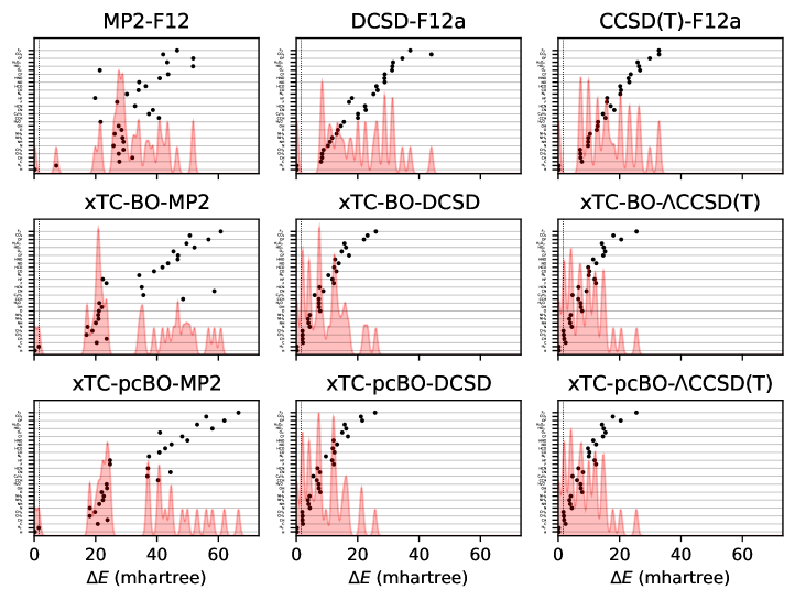
Fig.  1: Errors in total energies of the atoms and molecules from the HEAT dataset, calculated using aug-cc-pVTZ basis set. The errors are calculated with respect to the extrapolated FCI/CBS limit from Ref. 115. BO and pcBO denote methods based on the biorthogonal orbital optimisation and biorthogonal pseudo-canonical orbital transformation, respectively. Dotted lines indicate chemical accuracy (1 kcal/mol). The shaded area corresponds to the sum of Gaussians centered at each data point, with the width chosen such that for equally spaced points the Gaussians would be to 95% contained within their respective intervals.

The total energy errors of the atoms and molecules from the HEAT dataset are shown in Figure 1 and the corresponding statistics in terms of mean-signed deviation (MSD), standard deviation (STD) and maximal deviation (MaxD) are summarised in Table 1. The biorthogonal orbital optimisation only slightly affects the accuracy of the xTC-DCSD method. Note that the xTC-DCSD on top of pseudo-canonicalised orbitals (xTC-pcBO-DCSD) yields exactly the same results as the original xTC-DCSD method, and therefore the xTC-DCSD results are not shown in the figure. In agreement with our previous xTC-CCSD and xTC-DCSD experience, the xTC-CCSD(T) total energies for both versions of biorthogonal orbital rotations are more accurate than CCSD(T)-F12 ones.

Table 1:  Statistical measures of errors in total energies (aug-cc-pVTZ basis) with respect to HEAT estimates, in millihartree.

Method	MSD	STD	MaxD
CCSD(T)-F12	16.4	8.7	32.9
DCSD-F12	20.0	10.9	44.0
MP2-F12	31.7	11.3	51.8
xTC-BO-$\Lambda$CCSD(T)	8.9	6.2	25.5
xTC-pcBO-$\Lambda$CCSD(T)	8.8	6.2	25.4
xTC-BO-DCSD	9.7	6.8	25.9
xTC-DCSD	9.4	6.6	25.7
xTC-BO-MP2	32.8	16.4	60.8
xTC-pcBO-MP2	33.7	16.7	66.5

Surprisingly, the transcorrelated MP2 total energies (both, xTC-BO-MP2 and xTC-pcBO-MP2) for some systems, e.g., F₂, CO₂ or OF, turn out to be noticeably less accurate than MP2-F12. This hints to a potential limitation of the Jastrow optimization based on the minimisation of the variance of the reference energy, Eq. (6), especially for perturbative methods: the expression, which looks very similar to the xTC-MP2 energy expression, Eq. (14), does not include the usual orbital-energy denominators, and as the result the integral contributions are weighted uniformly and not according to the importance in the correlation. Unfortunately, inclusion of the orbital energies into the VMC framework is not feasible, however, it is possible to optimize the Jastrow factors by using Eq. (14) directly, and we are currently investigating this approach in our laboratory.

High accuracy of the absolute energies does not necessarily translate into high accuracy of relative energies, which is much more important for applications. In the next sections we investigate the accuracy of transcorrelated methods based on biorthogonally optimised orbitals for computation of atomisation and formation energies.

4.2 Atomisation energies

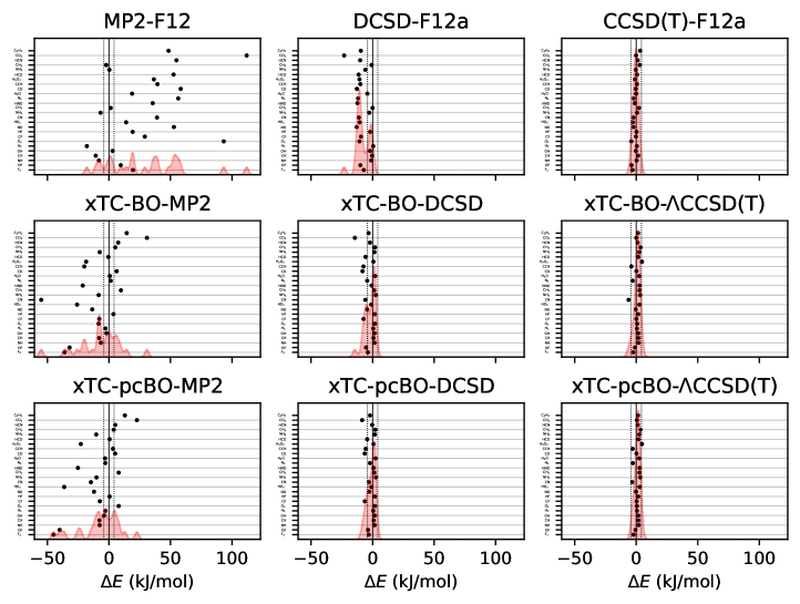
Fig.  2: Errors in atomisation energies of molecules from the HEAT dataset, calculated using aug-cc-pVTZ basis set. The errors are calculated with respect to the extrapolated FCI/CBS limit from Ref. 115. BO and pcBO denote methods based on the biorthogonal orbital optimisation and biorthogonal pseudo-canonical orbital transformation, respectively. Dotted lines indicate chemical accuracy (1 kcal/mol). The shaded area corresponds to the sum of Gaussians centered at each data point, with the width chosen such that for equally spaced points the Gaussians would be to 95% contained within their respective intervals.

The errors in atomisation energies of the molecules from the HEAT dataset are shown in Figure 2, and the corresponding statistics in terms of mean-absolute deviation (MAD), root-mean squared deviation (RMSD) and maximal deviation (MaxD) are summarised in Table 2.

Table 2:  Statistical measures of errors in atomisation energies (aug-cc-pVTZ basis) with respect to HEAT estimates, in kJ/mol.

Method	MAD	RMSD	MaxD
CCSD(T)-F12	1.47	1.90	-4.01
DCSD-F12	7.82	9.50	-23.13
MP2-F12	32.30	42.59	111.92
xTC-BO-$\Lambda$CCSD(T)	2.07	2.51	-6.20
xTC-pcBO-$\Lambda$CCSD(T)	1.94	2.24	4.63
xTC-BO-DCSD	3.56	4.74	-14.42
xTC-DCSD	2.69	3.35	-8.49
xTC-BO-MP2	13.61	18.78	-55.03
xTC-pcBO-MP2	12.40	17.31	-45.06

The biorthogonal orbital optimisation noticeably worsens the accuracy of the xTC-DCSD method, with RMSD increasing by 40%. As discussed in Section 2.1, the orbital optimisation changes the reference determinant and therefore the Jastrow factor is no longer optimal for the reference determinant of the coupled-cluster calculations, and the accuracy of the transcorrelated results can deteriorate.

The xTC-CCSD(T) atomisation energies are more accurate than the xTC-DCSD ones, and approach the accuracy of the CCSD(T)-F12 results. However, also in this case, the xTC-CCSD(T) method based on the biorthogonal orbital optimisation is less accurate than the one based on the pseudo-canonicalisation of the orbitals, although the difference is less pronounced than in the case of the xTC-DCSD method.

Interestingly, the xTC-MP2 atomisation energies are much more accurate than the ones obtained from MP2-F12. This is in contrast to the total energies, and suggests that the Jastrow factor optimisation based on the minimisation of the variance of the reference energy, Eq. (6), yields balanced Jastrow factors, even if they are not minimising the xTC-MP2 correlation energy contribution. Again, the xTC-MP2 results based on the biorthogonal orbital optimisation are less accurate than the ones based on the pseudo-canonicalisation of the orbitals.

4.3 Formation energies

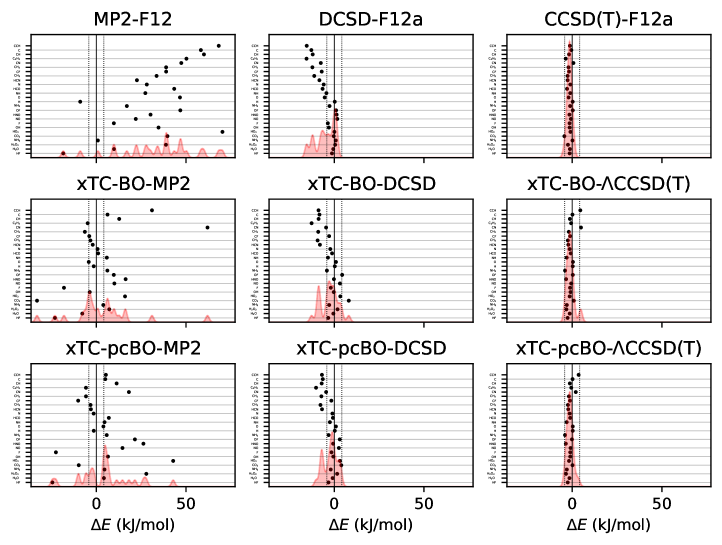
Fig.  3: Errors in formation energies of molecules from the HEAT dataset, calculated using aug-cc-pVTZ basis set. The errors are calculated with respect to the extrapolated FCI/CBS limit from Ref. 115. BO and pcBO denote methods based on the biorthogonal orbital optimisation and biorthogonal pseudo-canonical orbital transformation, respectively. Dotted lines indicate chemical accuracy (1 kcal/mol). The shaded area corresponds to the sum of Gaussians centered at each data point, with the width chosen such that for equally spaced points the Gaussians would be to 95% contained within their respective intervals.

Formation energies of the molecules from the HEAT dataset (see Table I from Ref. 101) have been calculated using the transcorrelated methods for biorthogonally optimised orbitals, and the errors with respect to the extrapolated full coupled cluster results at the complete basis set limit from Ref. 115 are shown in Figure 3. The statistics of the errors are summarised in Table 3.

Table 3:  Statistical measures of errors in formation energies (aug-cc-pVTZ basis) with respect to HEAT estimates, in kJ/mol.

Method	MAD	RMSD	MaxD
CCSD(T)-F12	1.60	1.89	-4.37
DCSD-F12	5.42	7.32	-15.47
MP2-F12	35.05	39.43	70.33
xTC-BO-$\Lambda$CCSD(T)	1.86	2.29	4.89
xTC-pcBO-$\Lambda$CCSD(T)	1.73	2.08	-4.02
xTC-BO-DCSD	4.40	5.58	-12.64
xTC-DCSD	3.47	4.40	-10.17
xTC-BO-MP2	11.57	17.55	61.99
xTC-pcBO-MP2	11.43	15.30	42.85

The results for the formation energies lead to similar conclusions as for the atomisation energies. The xTC-DCSD results on top of the biorthogonally optimised orbitals are less accurate than the original xTC-DCSD results, and the xTC-$\Lambda$CCSD(T) results are more accurate than the xTC-DCSD ones. As before, the sensitivity of the xTC-CCSD(T) results to the orbital optimisation is less pronounced compared to the xTC-DCSD results. The xTC-DCSD results are considerably more accurate than DCSD-F12, and the xTC-CCSD(T) results are close in the accuracy to the CCSD(T)-F12 results. The xTC-MP2 formation energies are much more accurate than the MP2-F12 ones, which again demonstrates the balanced description of the correlation by the Jastrow factors.

4.4 Effect of the xTC approximation

In order to investigate the accuracy of the xTC approximation, we have performed calculations of the total, atomisation, and formation energies using the xTC methods with the spin-averaged 1-RDMs, which yields spin-independent xTC integrals. In our previous calculations ¹⁰¹, we have found that xTC-DCSD based on the spin-independent xTC integrals are as accurate as the spin-dependent ones.

Table 4:  Statistical measures of errors in total, atomisation, and formation energies (aug-cc-pVTZ basis) with respect to HEAT estimates for xTC approximation using spin-averaged 1-RDMs.

Method	Total energy, mEh			Atomisation energy, kJ/mol			Formation energy, kJ/mol
	MSD	STD	MaxD	MAD	RMSD	MaxD	MAD	RMSD	MaxD
xTC-BO-$\Lambda$CCSD(T)	9.1	6.1	25.5	3.62	4.12	8.79	2.23	3.07	9.27
xTC-pcBO-$\Lambda$CCSD(T)	9.0	6.1	25.4	3.56	4.15	8.78	2.07	2.72	8.33
xTC-BO-DCSD	9.9	6.7	25.9	2.95	3.57	-8.78	3.26	4.18	10.29
xTC-DCSD	9.6	6.5	25.7	2.67	3.09	6.14	2.52	3.02	6.14
xTC-BO-MP2	33.0	16.3	60.8	13.21	18.04	-52.62	11.63	18.21	64.63
xTC-pcBO-MP2	34.0	16.6	66.5	12.03	16.47	-42.54	11.63	15.68	43.61

The statistics of errors in the total, atomisation, and formation energies of the atoms and molecules from the HEAT dataset are summarised in Table 4. The total energies of all methods are hardly affected by the different choice of the 1-RDMs in the xTC approximation. In agreement with our previous results, the relative xTC-DCSD energies based on xTC integrals calculated using the spin-averaged 1-RDMs are more accurate than the xTC-DCSD energies based on xTC integrals with the spin-resolved density matrices, and the biorthogonal orbital optimisation reduces the accuracy of the xTC-DCSD.

On the other hand, the xTC-CCSD(T) atomisation and formation energies are clearly less accurate when the spin-averaged-1-RDM based xTC integrals are used, and the accuracy of xTC-MP2 is comparable to the one based on the spin-resolved 1-RDMs. This suggests that the accuracy of the xTC approximation starts to become one of the limiting factors for the xTC-CCSD(T) method, and the choice of the 1-RDMs in the xTC approximation is important to obtain accurate results. The accuracy of the xTC approximation can be improved by using perturbative corrections to account for the missing explicit three-body terms in the xTC Hamiltonian, however, this would require a substantial increase in the computational cost of the xTC integrals.

4.5 Frozen-core calculations

One of the advantages of the transcorrelated methods based on optimised Jastrow factors is the possibility to perform calculations with frozen-core approximation with minimal loss of accuracy, as has been demonstrated for the xTC-DCSD method in Ref. 101. On the other hand, Ammar et al. ¹⁰⁴ have shown that the accuracy of the frozen-core approximation in transcorrelated methods can be improved by using the biorthogonal orbital optimisation, and without the orbital optimisation the frozen-core approximation leads to large errors in the transcorrelated methods with atomic Jastrow factors. Thus, to assess the effect of the biorthogonal orbital optimisation on the accuracy of the frozen-core calculations, we have performed such calculations of the total, atomisation, and formation energies of the atoms and molecules from the HEAT dataset using the xTC methods. The core electrons were frozen after the orbital optimisation, and we compare the results with the ones without the orbital optimisation and with the F12 results. The statistics of the errors are summarised in Table 5.

Table 5:  Statistical measures of errors in total, atomisation, and formation energies (aug-cc-pVTZ basis) with respect to HEAT estimates for frozen-core calculations.

Method	Total energy, mEh			Atomisation energy, kJ/mol			Formation energy, kJ/mol
	MSD	STD	MaxD	MAD	RMSD	MaxD	MAD	RMSD	MaxD
CCSD(T)-F12	95.3	44.4	194.0	5.47	6.53	-12.78	1.91	2.57	-7.05
DCSD-F12	98.7	46.7	204.9	12.79	15.16	-35.50	3.68	4.80	-12.02
MP2-F12	110.7	45.9	203.0	29.77	38.87	102.26	34.85	39.03	70.84
xTC-BO-$\Lambda$CCSD(T)	12.6	7.1	28.9	2.88	4.01	-10.81	2.10	2.38	3.88
xTC-pcBO-$\Lambda$CCSD(T)	10.8	6.2	25.5	2.19	2.88	-7.40	2.03	2.21	-3.50
xTC-BO-DCSD	13.4	7.9	31.1	5.68	7.63	-20.84	5.00	6.39	-15.06
xTC-pcBO-DCSD	11.3	6.7	25.8	3.91	5.20	-12.43	3.75	4.87	-12.17
xTC-DCSD	11.3	6.7	25.8	3.79	5.06	-12.13	3.68	4.80	-12.02
xTC-BO-MP2	36.1	17.6	64.0	14.14	19.74	-58.42	11.69	17.59	61.73
xTC-pcBO-MP2	34.9	16.8	65.5	12.38	17.56	-45.83	11.55	15.46	42.91

For the frozen core calculations xTC-pcBO-DCSD and xTC-DCSD results differ from each other, but only slightly, which suggests that the core orbitals and the remaining occupied orbitals are not strongly mixed in the pseudo-canonicalisation of the orbitals. Comparing the xTC-DCSD results among themselves, the biorthogonal orbital optimisation does not improve the accuracy of the frozen-core approximation in our calculations; on the contrary, the difference in the accuracy of the all-electron xTC-DCSD and xTC-BO-DCSD results is smaller, than the difference in the accuracy of the frozen-core xTC-DCSD and xTC-BO-DCSD results. It means that also in this case the biorthogonal orbital optimisation does not help to improve the accuracy of the transcorrelated calculations. Again, we attribute this to the fact that our Jastrow factors are optimised for the molecules according to Eq. (6), and the orbital optimisation changes the reference determinant.

Atomisation energies from the frozen-core xTC-MP2 method with pseudo-canonical orbitals approach the accuracy of the frozen-core DCSD-F12, but the formation energies are less accurate. Nevertheless, the frozen-core xTC-MP2 results are much more accurate than the frozen-core (and all-electron) MP2-F12 results.

The xTC-CCSD(T) results based on the pseudo-canonicalised orbitals are the most accurate ones among all methods employed in these frozen-core calculations. Compared to the all-electron xTC-CCSD(T) results, the accuracy of the frozen-core xTC-CCSD(T) results is slightly worse, but still better than the accuracy of the frozen-core CCSD(T)-F12 results.

5 Conclusions

In this work, we have investigated the effect of the biorthogonal orbital optimisation on the accuracy of the transcorrelated methods based on the xTC approximation and Jastrow factors optimised for the reference determinant through the minimisation of the variance of the reference energy. Additionally, we have investigated the accuracy of the xTC approximation in the combination with Møller-Plesset perturbation theory based methods, MP2 and CCSD(T). For CCSD(T) on the xTC Hamiltonian, we have employed the $\Lambda$CCSD(T) method, which is very similar to the standard CCSD(T) method, but does not rely on the hermiticity of the Hamiltonian.

In all our benchmark calculations, the biorthogonal orbital optimisation has not improved the accuracy of the xTC based coupled-cluster methods, and in most cases it has even worsened the accuracy of the transcorrelated results. This can be attributed to the fact that the Jastrow factors are optimised for the reference determinant, to minimise the residual correlation with respect to this determinant, and the orbital optimisation changes the reference, and therefore the Jastrow factors are no longer optimal for the reference determinant of the coupled-cluster calculations.

As an alternative to the biorthogonal orbital optimisation, we have investigated the pseudo-canonicalisation of the orbitals, and found that the xTC-CCSD(T) results based on the pseudo-canonicalised orbitals are more accurate than the ones based on the biorthogonally optimised orbitals, and are on par with the CCSD(T)-F12 results. Obviously, the higher excitations are included into the coupled cluster method, the less sensitive the results are to the orbital optimisation, and the xTC-CCSD(T) results based on the pseudo-canonicalised orbitals are much closer in the accuracy to the orbital-optimised xTC-CCSD(T) results, than in the case of the xTC-DCSD results.

As in our previous work, ¹⁰¹ the frozen-core xTC results are very accurate for all methods, and the xTC-$\Lambda$CCSD(T) results based on the pseudo-canonicalised orbitals are the most accurate ones among all methods employed in this work. The biorthogonal orbital optimisation does not improve the accuracy of the frozen-core calculations. This is in contrast to the results of Ammar et al. ¹⁰⁴, who have used atomic Jastrow factors, and found that the biorthogonal orbital optimisation greatly improves the accuracy of the frozen-core calculations.

The xTC-MP2 results are generally much more accurate than the MP2-F12 results, however, total energies of some molecules are less accurate than the MP2-F12 ones. This suggests that the Jastrow factor optimisation based on the minimisation of the variance of the reference energy, Eq. (6), can be improved by including the orbital energies as the weights for the integral contributions, which would lead to minimisation of the xTC-MP2 correlation energy, Eq. (14), and we are currently investigating this approach.

The somewhat sobering results of the xTC approximation in the combination with the CCSD(T) method compared to the all-electron CCSD(T)-F12 results, suggest that there is still room for improvement of the xTC approximation and the Jastrow factor optimisation. The accuracy of the xTC approximation is one of the limiting factors for the xTC-CCSD(T) method, and the choice of the 1-RDMs in the xTC approximation is important to obtain accurate results. Besides, the stochastic errors in the VMC calculations for the Jastrow optimisation lead to non-systematic errors in the final energies and the worse error cancellation in the relative energies.

The new implemented xTC-$\Lambda$CCSD(T) method will be useful to investigate the accuracy of the alternative ways of optimising the Jastrow factors and improving the xTC approximation. The biorthogonal orbital optimisation can become important in the cases where the Jastrow factors are not optimal for the reference determinant of the subsequent coupled cluster methods, e.g., for transferable Jastrow factors which can benefit more from error cancellation in the relative energies, and we are currently working on such an approach in our laboratory.

Conflicts of interest

There are no conflicts to declare.