An Investigation of the Current Star Formation Rate
of Star-forming Galaxies at z < 0.5 with FADO

Abstract

The star formation rate (SFR) is a crucial astrophysical tracer for understanding the formation and evolution of galaxies, determining the interaction between interstellar medium properties and star formation, thereby inferring the evolutionary laws of cosmic star formation history and cosmic energy density. The mainstream approach to study the stellar content in galaxies relies on pure stellar population synthesis models. However, these methods fail to account for the contamination of SFR caused by nebular gas radiation. Recent studies have indicated that neglecting nebular radiation contamination appears to be non-negligible in galaxies with intense star-forming activities and at relatively high redshifts, potentially leading to overestimation of stellar masses. However, there is currently limited targeted research, particularly regarding galaxies at higher redshifts (z $<$ 0.5). In this investigation, we employ the BPT diagram to select a sample of 2575 star-formation galaxies (SFG) from the SDSS-DR18 dataset, all within specified signal-to-noise ratio (S/N) ranges. Using the spectroscopic fitting tool FADO, which is capable of excluding nebular radiation contributions in spectral fitting, we conduct a tentative investigation of the SFR of star-forming galaxies in SDSS-DR18 with redshifts z $<$ 0.5. Our results show that 45$\%$ of the samples show H${\alpha}\lambda$6563 obtained from FADO fitting to be smaller than that derived solely from the pure stellar population synthesis model qsofitmore, particularly pronounced between redshifts 0.2 and 0.4. After calculating the SFR from H${\alpha}\lambda$6563 luminosity, we find that the contribution of nebulae is significant and exhibits an evolutionary trend with redshift, consistent with recent speculative findings. We anticipate that by combining optical and near-infrared spectral data, the influence of nebulae may become more prominent in star-forming galaxies at higher redshifts (e.g., up to z $\sim$ 2).

1 Introduction

The star formation rate (SFR), particularly the instantaneous SFR (SFR(t)), serves as a significant tracer for tracking stellar formation activities in galaxies, understanding their evolutionary history, and elucidating galaxy chemical evolution (Zhuang & Ho, 2019). It characterizes the rate at which new stars form within galaxies, thereby influencing their mass, type, and morphology. By combining observations of SFR with galaxy evolution simulations, the dominant physical processes driving galaxy growth can be thoroughly understood. For instance, processes such as galaxy quenching, gas accretion, star formation, and feedback from supernovae and active galactic nuclei (AGN) (Krumholz et al., 2012; Mullaney et al., 2012). Stellar formation represents the end point of a series of physical processes. Initially, gas cools from the interstellar medium and accretes onto the disk, forming a cold ‘atomic phase’, which then contracts into gravitationally bound clouds. Subsequently, molecular and molecular clouds form, dense clumps develop within molecular clouds, eventually leading to the formation of protostellar cores, stars, and star clusters. Although the starting and ending points of this process are relatively clear, the sequence of intermediate steps, especially the roles of forming cold atomic gas, molecular gas, and bound clouds, remains unclear, with different processes potentially dominating at different stages (Kennicutt & Evans, 2012). Investigating the influence of nebulae on SFR in galaxies contributes to inferring how gas affects the stellar formation process within galaxies and describing the conditions that compel gas to form stars. With increasingly reliable and precise estimations of SFR in galaxies and the discovery of numerous high-redshift galaxies by JWST, academic interest in researching SFR continues to soar. This has led to a burgeoning investigation into the relationship between redshift and SFR, sparking further inquiries in the field.

SFR also holds significant implications for a broad range of astrophysical studies. The Logarithmic linear relationship between stellar mass and SFR, known as the star-forming main sequence (SFMS) (Noeske et al., 2007), aids in understanding the trajectory of stellar activities in the Hertzsprung-Russell (HR) diagram and analyzing the characteristics of stars during the main sequence phase (Tacconi et al., 2020). SFR is crucial for cosmological reionization studies. When the first batch of O-type stars (Pop III) formed in the universe, primarily composed of hydrogen and helium, their intense radiation led to cosmic reionization. Accurate SFR estimation is also vital for studying the cosmic microwave background (CMB) radiation. By measuring SFR at different epochs in cosmic history, the contribution of various types of galaxies to the cosmic background radiation can be estimated, thereby refining cosmological ionization models and searching for the Pop III in the universe (Madau & Dickinson, 2014). Therefore, relatively precise SFR measurements are beneficial for various properties in astrophysics.To date, numerous large-scale astrophysical projects have been related to SFR. For instance, variations in SFR during the formation of star clusters and massive stars in different environments (Lada & Lada, 2003; McKee & Tan, 2002; Kirk et al., 2015; McKee & Ostriker, 2007); the promotion of SFR or black hole growth due to interactions between galaxies (Di Matteo et al., 2005; Springel et al., 2005); SFR corrections for cosmological reionization (Madau & Dickinson, 2014; Wang, 2013; Robertson & Ellis, 2012; Daigne et al., 2004); reevaluation of star formation within individual molecular clouds and gas relations (Kennicutt & Evans, 2012). Several large-scale surveys in astrophysics also focus on studying the properties of star-forming galaxies, such as the Sloan Digital Sky Survey (SDSS) (Peng et al., 2010), the Hubble Ultra Deep Field (HUDF) (Ellis et al., 2013), and the Atacama Large Millimeter Array (ALMA) (Wang et al., 2013).

Mainstream methods for estimating the SFR typically involve a fundamental step of spectral fitting for galaxies. This process entails fitting the spectrum as a combination of pure stellar population components, utilizing models based solely on stellar populations as templates for galaxy spectral fitting (e.g., STARLIGHT Cid Fernandes et al., 2005), Ppxf (Cappellari & Emsellem, 2004), qsofitmore (Fu, 2021). Considering that SDSS galaxies exhibit minimal nebular radiation due to insignificant star-forming activities, the aforementioned approaches overlook the modeling of nebular gas (Miranda et al., 2023), thereby neglecting the influence of nebular emission (Miranda et al., 2023; Ahumada et al., 2020). The limitation of these pure stellar models lies in their inability to solve different processes of gas emission within galaxies, as they incorporate assumptions that combine stellar mass, gas mass, and dust mass into a singular framework. However, studies by Krueger et al. (1995) and Salim et al. (2007) indicate that vigorous star-forming activities can lead to the nebular continuum contributing approximately 30%-70% to optical and near-infrared emissions, with nebular emission around star-forming regions accounting for about 60% of the total emission (Schaerer & de Barros, 2009; Krumholz et al., 2012). Therefore, when the acquired galaxy spectrum contain star-forming regions within the galaxy, the influence of nebulae becomes more pronounced. Pacifici et al. (2015) demonstrated that neglecting nebular emission in spectral modeling could lead to an overestimation of SFR by approximately 0.12 dex. Ignoring the contribution of nebular continuum would result in larger stellar mass and shallower ultraviolet slopes (Izotov et al., 2024). Galaxy evolution is primarily driven by the transformation of interstellar gas into stars, gas accretion between galaxies, intergalactic gas collisions, and galaxy mergers (Scoville et al., 2023). Thus, it is evident that interstellar gas plays a crucial role in the evolution of stars. FADO presents a viable solution for addressing the neglect of nebular emission in spectral processing. As the first independent and self-consistent spectral fitting tool to simultaneously consider stellar and nebular components in galaxies, FADO accounts for the impact of nebulae on SFR, dynamically and synchronously decomposing and calculating the contributions of different components and radiation mechanisms within the entire galaxy spectrum (Gomes & Papaderos, 2017). Therefore, in this investigation, we employ FADO as a research tool to consider nebular emission.

In this survey, we selected spectra of galaxies with active star formation at relatively high redshifts (z $<$ 0.5) from SDSS-DR18. These spectra were fitted using the FADO software and the Python toolkit qsofitmore, based on stellar population synthesis models. The aim was to explore whether nebular emission would interfere with the intrinsic estimation of SFR in galaxies at higher redshifts. H${\alpha}\lambda$6563 and H${\beta}\lambda$4861 are commonly regarded as the most reliable estimators of SFR, with Sobral et al. (2013) subsequently demonstrating the usefulness of H${\alpha}$ up to at least z $<$ 2.2. However, more extensive consideration of the [O II]$\lambda$3728 line is required around z $\sim$ 0.5, which can serve as an estimator of SFR up to z $<$ 1.4 (Kewley et al., 2004). SFR below z $<$ 0.4 can be accurately traced by H${\alpha}$ (Kennicutt, 1998), moderate redshift SFR by [O II]$\lambda$3728 (Kewley et al., 2004), and high redshift SFR by [O III]$\lambda$5007 (Shapley et al., 2023). Compared to the rough estimate of SFR provided by [O II]$\lambda$3728, H${\alpha}\lambda$6563 entails fewer assumptions, smaller uncertainties, and more accurate constraints on star-forming regions, making it the most accurate tracer of SFR to date (Kennicutt & Evans, 2012). However, H${\alpha}\lambda$6563 imposes strict constraints on redshift due to its longer wavelength, which may result in redshifts between 0.4 and 0.5 being beyond the observable wavelength range of the largest SDSS telescopes. Detailed analysis will be presented in Section 2.1. Furthermore, stellar age can be traced by the Balmer discontinuity at 3646 Å and the 4000 Å break; Si$\lambda$4128 and Cii$\lambda$1336 can track gas outflows or inflows; Mg$\lambda$2796 and [O iii]$\lambda$5007 can also estimate stellar metallicity and temperature (Förster Schreiber & Wuyts, 2020).

Several studies have recently demonstrated the stability of FADO in spectral fitting and line information estimation. Breda et al. (2022) found, through comparison with STARLIGHT using simulated data, STARLIGHT overestimated the mass-weighted mean stellar age by up to $\sim$ 4 dex and the metallicity and light-weighted mean stellar age by up to $\sim$ 2 dex. Given these findings, they concluded that FADO can accurately recover mass, age, and mean metallicity with high precision ($\sim$ 0.2 dex). Furthermore, Cardoso et al. (2022) showed that for galaxies with EW (H_α) >3 $\AA$, the average mass and metallicity of the entire galaxy can differ by up to $\sim$ 0.06 dex, with a discrepancy of $\sim$ 0.12 dex. Most recently, Miranda et al. (2023) compared the SFR obtained from FADO fitting of the MPA-JHU galaxy sample with that obtained from STARLIGHT fitting of the MPA-JHU sample and found a difference of 0.01 dex in Ha flux between the two methods. They also predicted that nebular radiation not only plays a crucial role in the star formation activity of galaxies but also affects the calculation of galaxy SFR, particularly in high-redshift galaxies. In conclusion, the presence of nebulae does indeed affect the accurate estimation of SFR. Additionally, recent research by Izotov et al. (2024) has shown that neglecting the contribution of nebular continuum in determining SFR would result in larger stellar masses and shallower ultraviolet slopes. This is particularly significant for galaxies like J2229+2725, which are considered analogs of early-universe dwarf galaxies and play a role in cosmic reionization.

The purpose of this investigation is to simultaneously fit galaxy spectra using the pure stellar code qsofitmore and FADO, which considers the contribution of nebular continuum. By examining the differences in the H${\alpha}\lambda$6563 emission line in the fitted spectra, we aim to further determine the disparity in SFR. It is worth mentioning that based on the rough information available about stars in galaxies, stellar mass and SFR may not be sufficient to infer the potential evolutionary paths of galaxies. We still need to combine the spatial resolution information provided by all baryonic components of galaxies (stars, gas, metals) and the complete kinematic tracers of gravitational potential (dark matter), as well as the kinematic tracers of galaxy feedback processes (quenching, AGN, and supernova feedback), in order to obtain the complete evolutionary paths of galaxies (Förster Schreiber & Wuyts, 2020). Therefore, we remain open-minded regarding the derivation of galaxy evolution processes in the current scenario where we have no knowledge of dark matter.

Section 2 outlines the criteria for selecting sources in the galaxy spectroscopic analysis and the process of spectral fitting employed in this study. In Section 3, we present the statistical analysis of the selected sample and the main findings. Section 4 discusses four critical issues related to the spectroscopic data and fitting techniques employed in this investigation. Finally, Section 5 provides a summary of this preliminary research. Throughout the paper, we assume a standard cosmological model with Hubble constant $H_{0}$ = 72 km s^-1 Mpc^-1, matter density $\Omega_{M}$ = 0.3, and cosmological constant $\Omega_{\Lambda}$ = 0.7.

2 sample selection and spectral fitting

The galaxy sample and their spectra used in this investigation are selected from Sloan Digital Sky Survey Data Release 18th (SDSS-DR18, Almeida et al., 2023).It integrates data from the previous 17 data releases and incorporates new observational data and improvements. Spectra were retrieved from the optical spectroscopic section of the SDSS Science Archive Server (SAS) . We selected all galaxies with redshifts not exceeding 0.5, resulting in approximately 1.73 million samples.

2.1 Parent sample

To ensure reliable spectral fitting results, it is necessary to select samples with a sufficient S/N. Considering that FADO performs better in fitting spectra with median S/N > 5 compared to other pure stellar codes (Pappalardo et al., 2021), we first selected samples with a median S/N greater than 5. Furthermore, to effectively utilize high-quality spectra at arbitrary redshifts and ensure a uniform distribution of galaxy samples at different redshifts, we set an exponential curve (red solid line in Figure 1) and selected 36,109 galaxies with high S/N (blue scatter in Figure 1), constituting the parent sample. In fact, for the majority of spectroscopic surveys, there exists an inverse exponential relationship between the redshift of extragalactic sources and the maximum value of the spectroscopic S/N.As the redshift increases, the number of celestial objects captured by SDSS decreases(Almeida et al., 2023). Thus, this exponential curve is reasonable. The analytical expression of this curve is as follows:

$$y=e^{-((x-0.22)\cdot 5)\cdot 20}$$ (1)

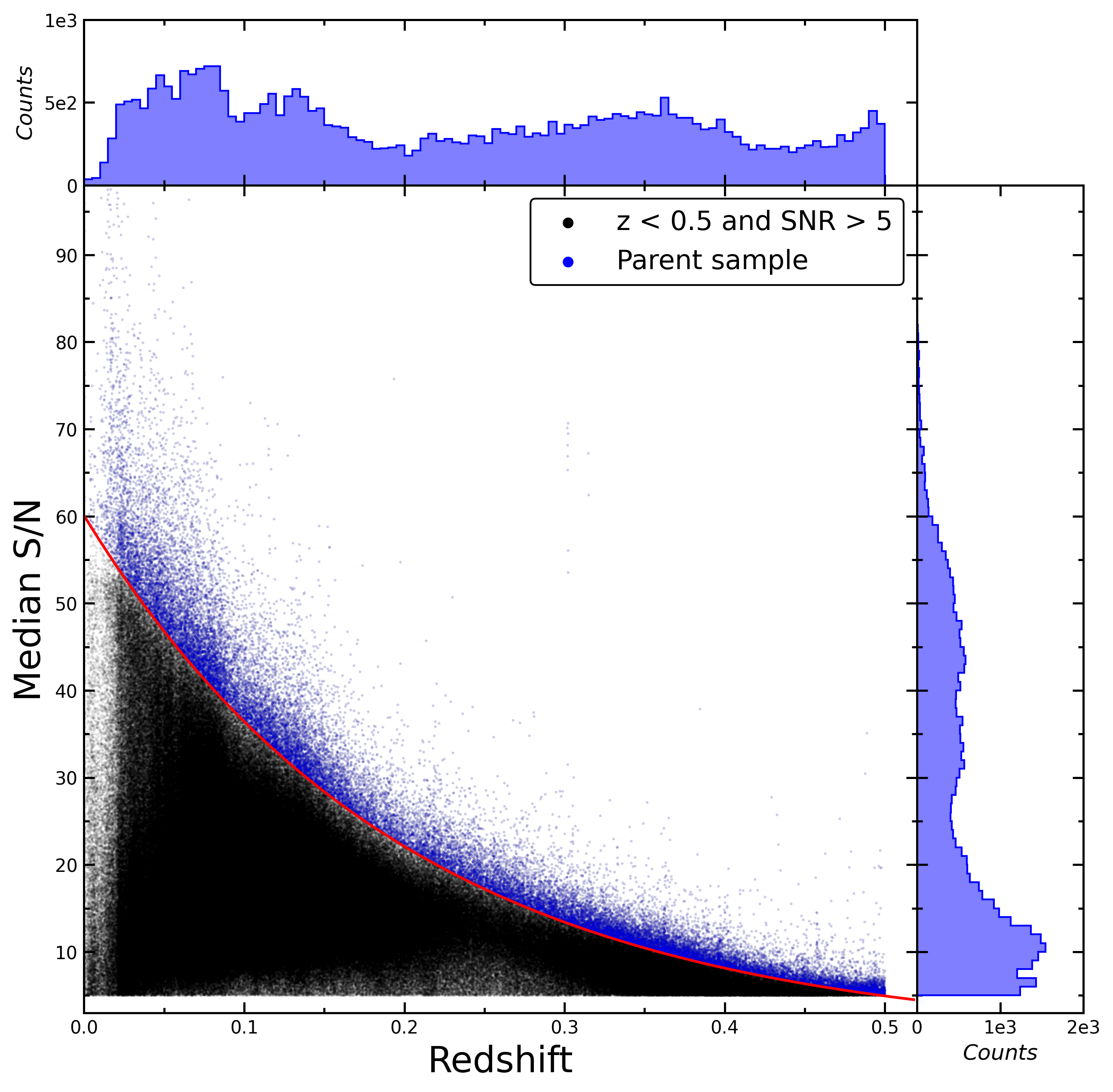
Figure 1: The median S/N of galaxy spectra in SDSS-DR18 across galaxy redshifts. The black dots represent a sample of galaxies with redshifts less than 0.5 and median S/N $>$ 5, while the blue dots denote the parent sample selected based on an exponential curve (see the text for details). The histograms in the upper and right panels illustrate the distribution of the number of galaxies in the parent sample as a function of redshift and median S/N in the spectra.

From the histogram in the upper panel of Figure 1, it can be seen that the distribution of the parent sample’s quantity versus redshift is relatively uniform. This ensures that our conclusions are not excessively affected by sample bias. However, as will be seen in the following two sections, further processing of the parent sample and stringent selection criteria inevitably result in the loss of a large number of samples, and even cause the extracted new samples to no longer be uniformly distributed with redshift. Nevertheless,the parent sample have to be addressed in depth to obtain a pure sample, that is, the gold sample. The parent sample have to be addressed in depth to obtain a pure sample.

2.2 BPT selection

The data selection in this survey involves classifying galaxies based on their positions on the BPT diagram. We utilize the BPT diagram based on four emission line ratios, namely [N II] $\lambda$6583, [O III] $\lambda$5007, $H\alpha$ $\lambda$6563, and $H\beta$ $\lambda$4861 (Baldwin et al., 1981). The selected data points are ensured to lie in the pure star-forming (SF) region of the BPT diagram, with S/N $>$ 5 and z $<$ 0.5. The two boundary lines in Figure 2 are derived from Equation 2 (Kewley et al., 2001) and Equation 3 (Kauffmann et al., 2003). These boundary lines divide the BPT diagram into three regions, where the blue represents star-formation galaxies, gray represents composite galaxies, and red represents AGN regions. Prior to inclusion in the BPT diagram, we carefully select galaxies from 36,109 with reasonable flux values for the aforementioned four emission lines, ensuring that these data points have physically meaningful positive fluxes. Subsequently, the galaxies selected as SF galaxies (SFG) are plotted on the BPT diagram to obtain the required SFG distribution, as depicted in Figure 2. A total of 2575 galaxies are ultimately identified as SFGs on the BPT diagram. These data points are then subjected to spectral fitting using qsofitmore and FADO to obtain the most accurate emission line fluxes.

$$\log\left(\frac{[\mathrm{O}\mathrm{III]}\lambda 5007}{\mathrm{H}\beta}\right)=\frac{0.61}{\log([\mathrm{N}\mathrm{II}]/\mathrm{H}\alpha)-0.47}+1.19,$$ (2)

$$\log([\mathrm{O}\mathrm{III]}/\mathrm{H}\beta)>0.61/\{\log([\mathrm{N}\mathrm{II}]/\mathrm{H}\alpha)-0.05\}+1.3.$$ (3)

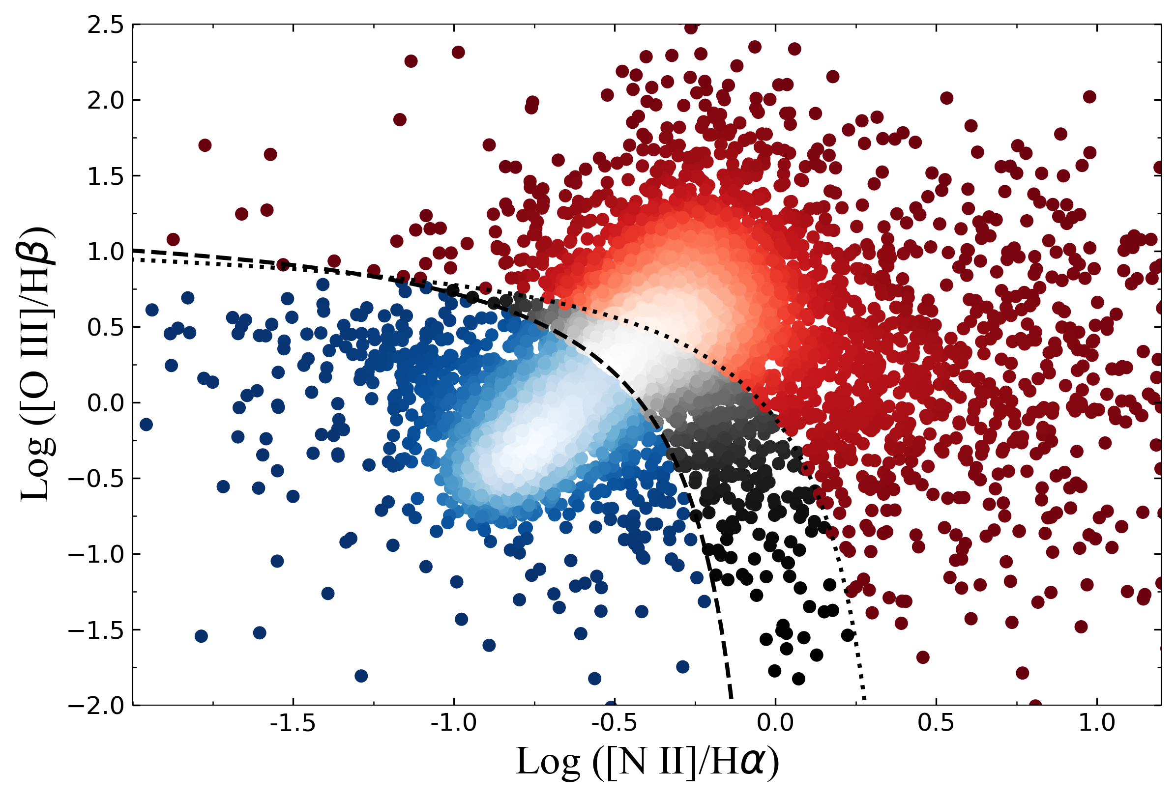
Figure 2: The result of BPT selection. Blue region represents star-formating galaxies, gray region represents composite galaxies, and red region represents AGN and Seyfert galaxies. The denser the data in the Figure, the brighter the corresponding color, and the sparser the data, the corresponding darker the color.

2.3 Spectral fitting

The PyQSOFit is a dedicated data package for fitting SDSS spectra, primarily used for fitting quasar spectra and calculating the central supermassive black hole masses in quasars. It can also be applied to galaxy spectra, such as for calculating the SFR of galaxies. Based on PyQSOFit, Fu (2021) improved it to become qsofitmore, which is no longer limited to fitting SDSS spectra but can be used to analyze spectral data files obtained from other devices, such as LAMOST. qsofitmore has shown good performance in spectral fitting and analysis and has become increasingly popular in quasar and galaxy spectral studies (Fu et al., 2022; Jin et al., 2023; Ding et al., 2023; Chen et al., 2024). This improved Python package not only fits the emission line information of target galaxy spectra but also uses Monte Carlo (MC) method to obtain the flux errors of the fitted components. It should be noted that qsofitmore is based on the BC03 model (Bruzual & Charlot, 2003) for spectral fitting, which does not simultaneously consider the radiations of stars and nebulae to decompose the spectral components, as FADO does. This allows us to compare the SFR obtained considering nebulae radiation in FADO with that obtained by qsofitmore to demonstrate whether there is a significant difference in higher redshifts.Additionally, in qsofitmore, we take into account the potential contamination of galaxy spectra by the host galaxy. Thus, we remove the contribution from the host galaxy to obtain smoother galaxy spectra. As shown in the appendix.

FADO is considered a self-consistent and dynamically calculated spectral fitting tool that takes into account the contribution of nebular radiation to emission line luminosities. FADO is the first population spectral synthesis(pss) code employing genetic differential evolution optimization. By identifying the main nebular features in galaxies through the observed Balmer line luminosities and equivalent widths (EWs), as well as the shape of the continuum around the Balmer and Paschen jump regions, FADO realizes the estimation of nebular emission lines. This is achieved through the full-consistency mode (FC), Nebular-Continuum mode (NC), and STellar mode (ST) (Gomes & Papaderos, 2017). The main difference between FADO and other pure stellar codes (such as STARLIGHT and qsofitmore) is that FADO considers the contribution of nebular emission lines in galaxies rather than solely estimating the SFR of the target galaxy using stellar radiation. The advantage of FADO lies in its ability to simultaneously fit and estimate multiple parameters, such as age, metallicity, stellar mass, and dust content in galaxies. This allows for a more comprehensive analysis of the physical properties of galaxies. Both qsofitmore and FADO use the MC method to assign spectral flux errors, and their basic template spectra are derived from the BC03 model. Additionally, they can both perform extinction correction, dereddening, and K-correction on spectra under given celestial coordinates and redshifts, ensuring comparability with the fitting of qsofitmore and maintaining control and uniformity in the basic spectral processing conditions.

Therefore, we conducted fittings on the spectra of 2575 galaxies obtained from Section 2.1 using FADO and qsofitmore, respectively, and conducted preliminary inspection and screening of the fitting results (e.g., fitted fluxes of H${\alpha}$ and H${\beta}$). In regions of active star formation, there are sufficiently young and hot stars that provide enough energy for the ionization of hydrogen. These ionized gases capture photons and undergo recombination transitions, leading to simultaneous emission of H${\alpha}$ and H${\beta}$. Additionally, the significant electromagnetic radiation emitted during star formation is heavily attenuated by dust obscuration. Since dust absorption and attenuation are more efficient at longer wavelengths than shorter ones, this results in a decrease in the H${\alpha}$-H${\beta}$ ratio (Calzetti et al., 2000). Theoretically, an H${\alpha}$-H${\beta}$ ratio of 2.86 is commonly regarded as a typical intrinsic extinction indicator reflecting the dust absorption effects on hydrogen emission lines (Hummer & Storey, 1987; Gaskell & Ferland, 1984). Therefore, we corrected for intrinsic extinction using an H${\alpha}$-H${\beta}$ ratio of 2.86 for all our data when calculating SFR (Cardelli et al., 1989). Both FADO and qsofitmore software come with Milky Way extinction corrections, thus intrinsic extinction correction for galaxies is necessary. The detailed procedure of the extinction correction is presented in the Appendix.

Table 1 shows five criteria were used to select galaxies suitable for subsequent analysis: (1) z < 0.5; (2) high spectral quality and appropriate S/N; (3) selection based on the BPT diagram; (4) successful fitting of H${\alpha}$; and (5) successful fitting of both main emission lines, H${\alpha}$ and H${\beta}$. Criterion (4) was employed to directly compare the differences in H${\alpha}$ fitting between the two spectral fittings without sacrificing too many samples. The distribution of this data is quantified in the Left panel of Figure 3. Criterion (5) was implemented to compare the differences in SFR between the two fittings. Before calculating SFR, intrinsic extinction correction is necessary to ensure the reliability of the estimated SFR, hence both H${\alpha}$ and H${\beta}$ needed to be successfully fitted. The distribution of this data is quantified in the Right panel of Figure 3. The corresponding selected samples consisted of 2575 and 2215 spectra, respectively. After excluding three outliers, we obtained a golden sample containing 2212 galaxy spectra, all of which met the requirements of this investigation. The complete spectral selection criteria and the resulting samples are presented in Table 1. For the estimation of SFR, the number of galaxies in the golden sample was 1807. The reason for sample loss was the intrinsic extinction correction, and the specific data are shown in Figure 8.A comparison of the emission line fittings between FADO and qsofitmore in criteria (4) and (5) reveals that FADO performed better, fitting more emission lines and reducing sample loss. It is worth noting that the last column in the table represents the number of samples that satisfied the corresponding criteria and were successfully fitted by both FADO and qsofitmore, which are the data truly used for sample selection in this study. During the selection process, the sharp decrease and scarcity of samples were greatly influenced by the fitting results of qsofitmore, as it imposes stricter criteria on spectral fittings. This indicates that compared to the recently developed FADO spectral fitting method, previous methods for fitting galaxy spectra have certain limitations under the assumption of reasonable and excellent spectral fitting capabilities of FADO. After obtaining the golden sample, necessary parameter comparative analyses were conducted, and the results are presented in the next section.

Table 1: The source selection criterion used in this investigation and the corresponding number of selected samples.

	Criteria	FADO	qsofitmore	Combined
(1)	SDSS-DR18   z $<$ 0.5	1,730,947	1,730,947	1,730,947
(2)	S/N above red line and z $>$ 5	36,109	36,109	36,109
(3)	BPT diagram selection	2,575	2,575	2,575
(4)	Hα fitted	2,575	2,212	2,212
(5)	Hα and Hβ fitted Final gold sample	2,563	1,807	1,807

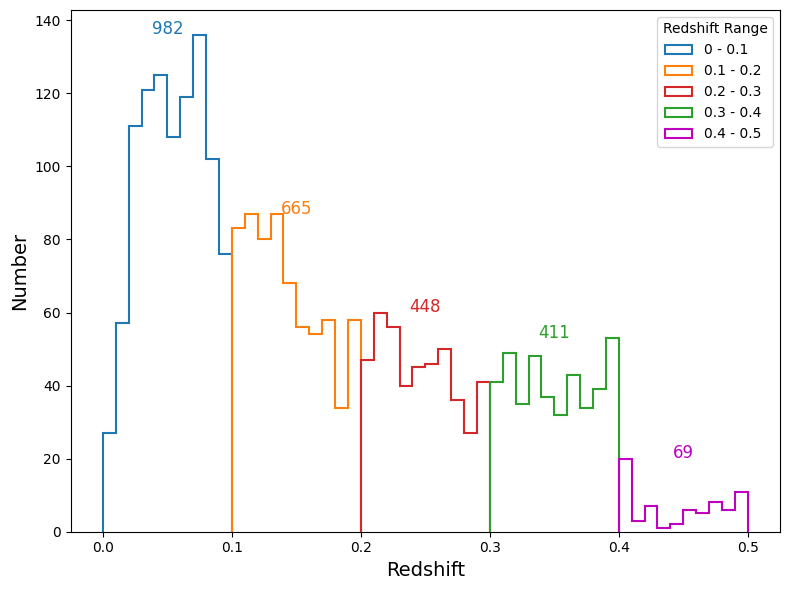
(a) BPT Selection

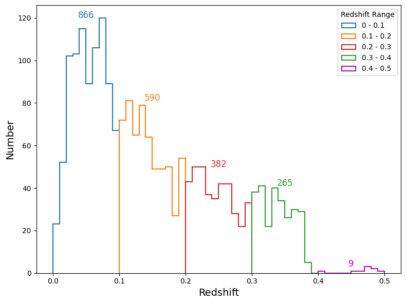
(b) H$\alpha$ Selection

Figure 3: Panel (a): Sample selected by BPT diagram, which contains 2575 galaxies binned by 0.1 in redshift. Panel (b): H$\alpha$ sample fitted by both FADO and qsofitmore after BPT diagram selection, which contains 2112 galaxies. The selection lead to a significant sample loss at $z>0.4$.

The distribution of data points in this survey with respect to redshift is illustrated in Figure 3. The left panel represents the data after BPT diagram selection, while the right panel depicts the subset that satisfies both the BPT diagram selection and the fitting of H${\alpha}\lambda$6563 lines. It is evident from both histograms that there is a declining trend, with a notable difference in the number of data points between the redshift intervals of 0-0.1 and 0.4-0.5. Despite the careful selection of an appropriate number of data points in each redshift interval in Figure 1, the discrepancy in the data is more pronounced in Figure 3. This is attributed to the fact that the redshift interval of 0-0.1 corresponds to nearby galaxies, which are typically well observed with advanced techniques and thorough research methods, resulting in higher-quality spectra that are less likely to be filtered out by FADO and qsofitmore. Conversely, the redshift interval of 0.4-0.5 exceeds the median redshift of the SDSS survey (around 0.1) (Abazajian et al., 2009), leading to a obviously drop in the data shown in Figure 3. Moreover, the requirement of simultaneously fitting [N II] $\lambda$6583, [O III] $\lambda$5007, H${\alpha}\lambda$6563, and H${\beta}\lambda$4861 lines in the BPT diagram poses a stringent constraint, particularly for the data in the 0.4-0.5 redshift range, especially for H${\alpha}\lambda$6563. Around a redshift of 0.5, H${\alpha}\lambda$6563 may fall beyond the maximum wavelength coverage of the SDSS, resulting in its failure to be fitted, thereby further reducing the data. The decrease in data in the right panel is due to the stringent fitting criteria of qsofitmore and FADO, which may erroneously fit flux values for some low-quality spectra, leading to data reduction. This reduction is particularly evident in the 0.4-0.5 redshift interval in the right panel, where most of the data are removed due to the fitting of H${\alpha}\lambda$6563 and H${\beta}\lambda$4861 lines. Consequently, the main focus of this investigation is on the sample concentrated between 0 and 0.4, as the data in the 0.4-0.5 interval are sparse. However, there are better data trends in the following figures, which will be shown in next section.

3 results and analysis

The purpose of this investigation is to compare the SFR derived from qsofitmore and FADO, aiming to evaluate whether FADO can provide a more reasonable SFR by excluding nebular contamination. As mentioned in Section 2.2, H${\alpha}\lambda$6563 is currently considered the most suitable estimator for galaxy SFR. Therefore, this investigation utilizes the H${\alpha}\lambda$6563 luminosity to calculate the SFR of the golden sample. Equation 4 and Equation 5 are employed to compute the optimal SFR values.

$$L(\mathrm{H}\alpha)=F(\mathrm{H}\alpha)4\pi d_{L}^{2}$$ (4)

$$\mathrm{SFR}=\frac{L(\mathrm{H}\alpha)}{\eta(\mathrm{H}\alpha)}$$ (5)

Where $d_{L}$ is the luminosity distance, $F\ {(H\alpha)}$ the best fitted flux of after extinction of H${\alpha}\lambda$6563, $L\ {(H\alpha)}$ the luminosity of $H\alpha\lambda$6563 and $\eta(\mathrm{H}\alpha)=10^{41.28}\mathrm{erg}\mathrm{s}^{-1}M_{\odot}^{-1}\mathrm{yr}$, the multiplication factor given by (Miranda et al., 2023).Calibrated to (Chabrier, 2003) IMF. Among them, qsofitmore and FADO use consistent calibration and consistent calculation methods to calculate SFR.

The estimation results indicate that FADO yields SFR values for the golden sample, which are statistically nearly half of those provided by qsofitmore. As illustrated in Figure 4, 950 galaxies (45%) exhibit lower SFR values from FADO compared to those from qsofitmore. The black dashed line in the figure represents equality between the SFR values obtained from both methods, with error bars derived using Monte Carlo methods. The top panel comprises five subplots quantifying the comparison of fits across different redshift intervals, where the black dashed line signifies equality between the two fitting tools. Top panel of Figure 4 shows a good trend of changes with redshift. It can be seen that from z = 0-0.1 to z = 0.3-0.4, as the redshift increases, the black dotted line have more and more data under, which shows that more and more data points indicate that H${\alpha}\lambda$6563 fitted by FADO is smaller than H${\alpha}\lambda fittedby{\it qsofitmore}$6563.This aligns with our expectation since qsofitmore, in computing SFR, does not account for the nebular component, thus overestimating the emission intensity from star-forming activities, leading to inflated SFR estimates. Figure 5 quantifies all data points below the diagonal line, with the redshift range of 0.2-0.4 exhibiting notable differences, with approximately 69% of the data falling below the qsofitmore fit. Figure 5 preliminarily demonstrates the sensitivity of the SFR derived from FADO fits to the H${\alpha}\lambda$6563 line in the range of z = 0.2 $\sim$ 0.4, consistent with the inference by Miranda et al. (2023). However, it is crucial to note that our sample remains too limited, particularly in the redshift range of 0.4-0.5. This limitation arises partly due to the selected redshift range, preventing us from obtaining a sufficient number of spectroscopic parent samples solely from SDSS optical spectra for fitting. Additionally, the suboptimal spectral observation quality of galaxies within the chosen redshift range by SDSS leads to the exclusion of the majority based on criterion (4) (see Section 2.1). Thus, more high-quality spectra are needed to be collected to expand the golden sample, to better elucidate the trends depicted in Figure 5. Furthermore, during the spectral fitting stage, we observed that qsofitmore imposes stringent conditions on spectral fitting, with the majority of spectra failing to exhibit the emission lines that should ideally be present, possibly due to the SED fitting model used as a reference by qsofitmore (Fu, 2021). The high requirements for spectral quality by qsofitmore also contribute significantly to the scarcity of the golden sample. Additionally, we conducted a KS test on the x and y coordinates of Figure 4 to assess whether they follow the same distribution. The KS statistic: 0.178, P-value: 2.01E-32, indicates a significantly small P-value, suggesting significant distributional differences between the two datasets. The Ha emissions fitted by qsofitmore and FADO do not conform to the same distribution.

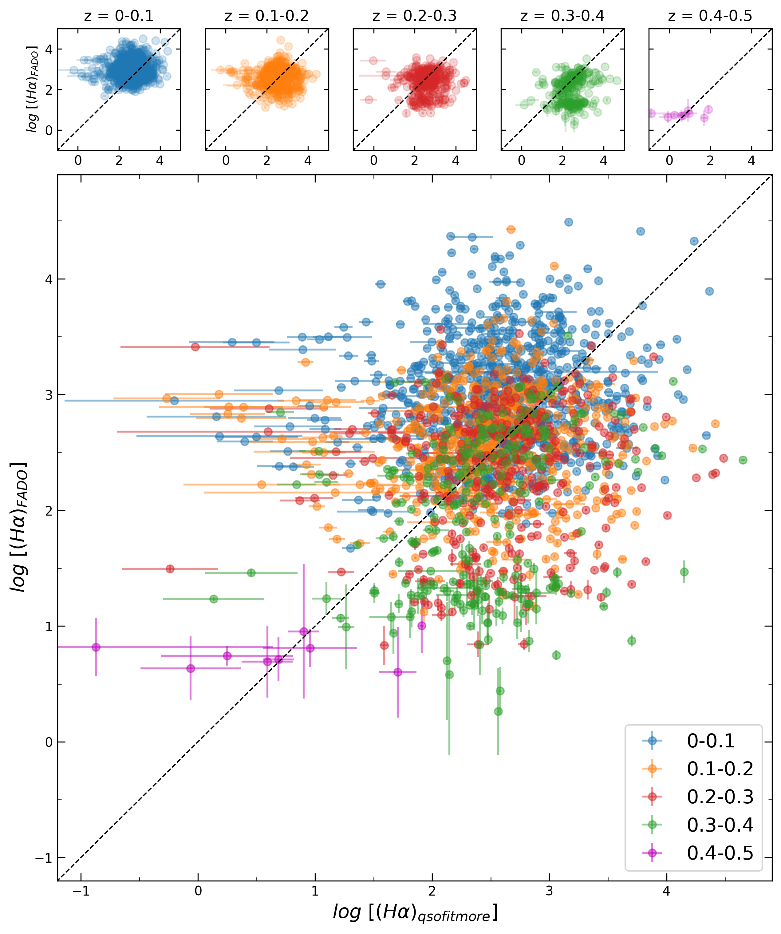
Figure 4: The H$\alpha$ flux fitted by qsofitmore across that of FADO. Both of them are logarithmized. Uncertainties are given by Monte Carlo in both fitting. The five upper panels show the scatter for each redshift bin.

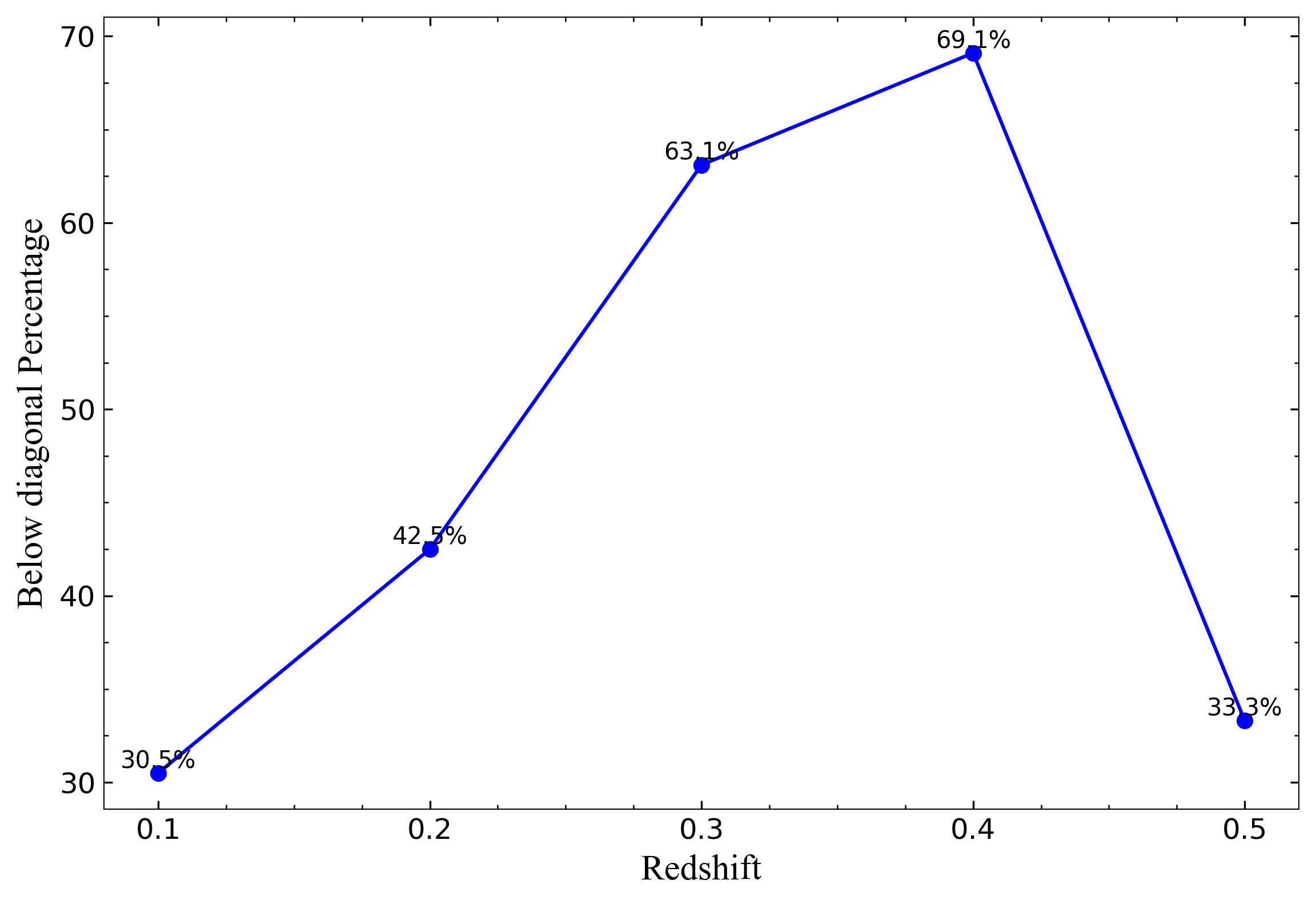
Figure 5: All data distribution below the diagonal. All data inherit the errors of the two softwares, allowing for more accurate analysis. The abscissa represents the redshift, and the ordinate represents the scale below the diagonal. It can be seen that there are more data below the diagonal in the range of redshift 0.2-0.4, while there are less data in the redshift 0.1 and redshift 0.5 range.

To further investigate the trend of the ratio of H${\alpha}\lambda$6563 fluxes from FADO and qsofitmore with redshift, we present in Figure 6 the relationship between the ratio of H${\alpha}\lambda$6563 fluxes and redshift. Since the calculation of SFR in this study is based on the H${\alpha}\lambda$6563 emission line luminosity, to avoid reducing our parent sample due to the joint fitting of H${\alpha}\lambda$6563 and H${\beta}\lambda$4861, we adopt the H${\alpha}\lambda$6563 / H${\beta}\lambda$4861 ratio to quantitatively characterize the extent of bias introduced by the nebular component to SFR estimation in past studies. The relationship between this ratio and redshift can reveal how the contribution of nebular radiation to galaxy emission changes with increasing redshift. After linearly fitting the sample, we found a slight decrease in the vertical axis with increasing redshift. This may suggest that at higher redshifts, the effect of nebulae on SFR estimation becomes more pronounced, consistent with the inference of (Miranda et al., 2023). However, due to the narrow range of selected redshifts and the small sample size, this trend is not apparent. Therefore, more high-quality spectra of intermediate to high-redshift galaxies are needed in the future to amplify this trend and verify the universality of this phenomenon. The large error in the data in Figure 6 may be attributed to the significant estimation error resulting from FADO’s use of a Monte Carlo code combined with many models, which will be analyzed in the next section. It can be observed from Figure 6 that regardless of whether errors are included, the final slope is negative, indicating a decrease in the vertical axis with increasing horizontal axis. The decrease in the vertical axis implies that $H_{\text{FADO}}$ is overall smaller than $H_{\text{{\it qsofitmore}}}$, which is consistent with our initial speculation. This is because FADO removes some radiation originally from nebulae when fitting the H${\alpha}\lambda$6563 emission line, fitting only the radiation from stars, resulting in a more accurate and smaller flux.

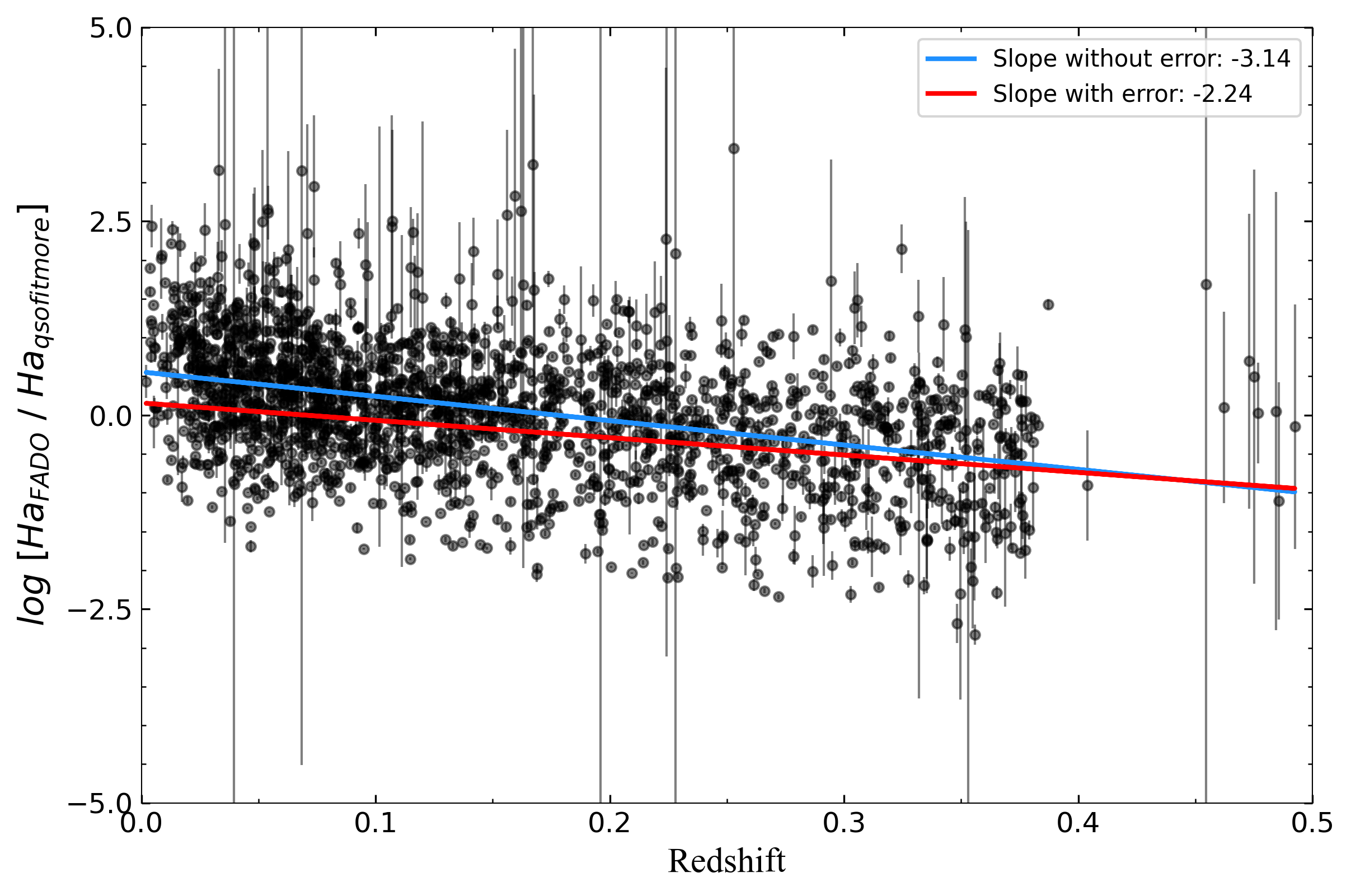
Figure 6: Trend of the ratio of H${\alpha}\lambda$6563 from FADO and qsofitmore with redshift. The red solid line represents the fitting without error, with a slope of -2.24; the blue solid line represents the fitting without error, with a slope of -3.14. It shows that as the redshift increases, $H\alpha_{FADO}/H\alpha_{\it qsofitmore}$ tends to decrease slightly, implying that the nebular radiation may become increasingly significant at high redshift.

Next, we attempt to quantify the differences between the two fitting methods in computing SFR. They employ the same formula for SFR calculation, as shown in Equation 4 and Equation 5, thus ensuring comparability of the SFR calculation data. The intrinsic extinction correction of galaxies has been considered in the SFR calculation, and detailed methods are provided in the Appendix. The SFMS (star-forming main sequence) is plotted against stellar mass, which is estimated by FADO. There exists a close relationship between stellar mass and SFR, with current research indicating a positive linear logarithm relationship. Since SFR calculations are based on extinction-corrected data, both and H${\beta}\lambda$4861 need to be fitted simultaneously by both methods. This requires a re-evaluation of the data, and Figure 7 depicts the scenario where both H${\alpha}\lambda$6563 and H${\beta}\lambda$4861 are fitted. It can be observed that there are very few data points remaining in the redshift range of 0.4-0.5, which can be almost neglected. This is due to the stringent fitting criteria of FADO and qsofitmore, coupled with the poor spectral quality in the redshift range of 0.4-0.5, which is insufficient to meet the requirements of this study. The left panel of Figure 8 illustrates the SFMS diagram from FADO, while the right panel shows the SFMS diagram from qsofitmore. The two lines in Figure 8 represent the slopes of the SFR calculated by FADO and qsofitmore, respectively. To facilitate comparison of their differences, these two slopes are juxtaposed. The data from this survey also adhere to the SFMS relationship established by other researchers, where the overall SFR increases with increasing stellar mass. However, we observe that the amplitude of SFR calculated by FADO increases much more rapidly with increasing stellar mass compared to that calculated by qsofitmore. The SFR calculated by FADO tends to align more closely with a proportionate upward trend, whereas that by qsofitmore tends to approach a straight line. This indicates that the SFR calculated by FADO exhibits a better trend, capturing a flux of H${\alpha}\lambda$6563 that conforms more closely to theoretical models of the SFMS trend, further underscoring the robustness of FADO. The right panel of Figure 8 displays the SFR calculated by qsofitmore, indicating almost no upward trend, with data distribution tending towards a flat line and lacking a discernible linear trend, contrary to the SFMS prediction by FADO.

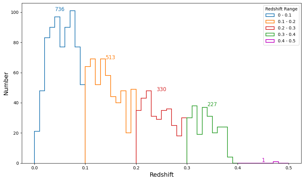
Figure 7: The data distribution of H${\alpha}\lambda$6563 and H${\beta}\lambda$4861 fitted by two methods. There is very little data for redshift 0.4 to 0.5.

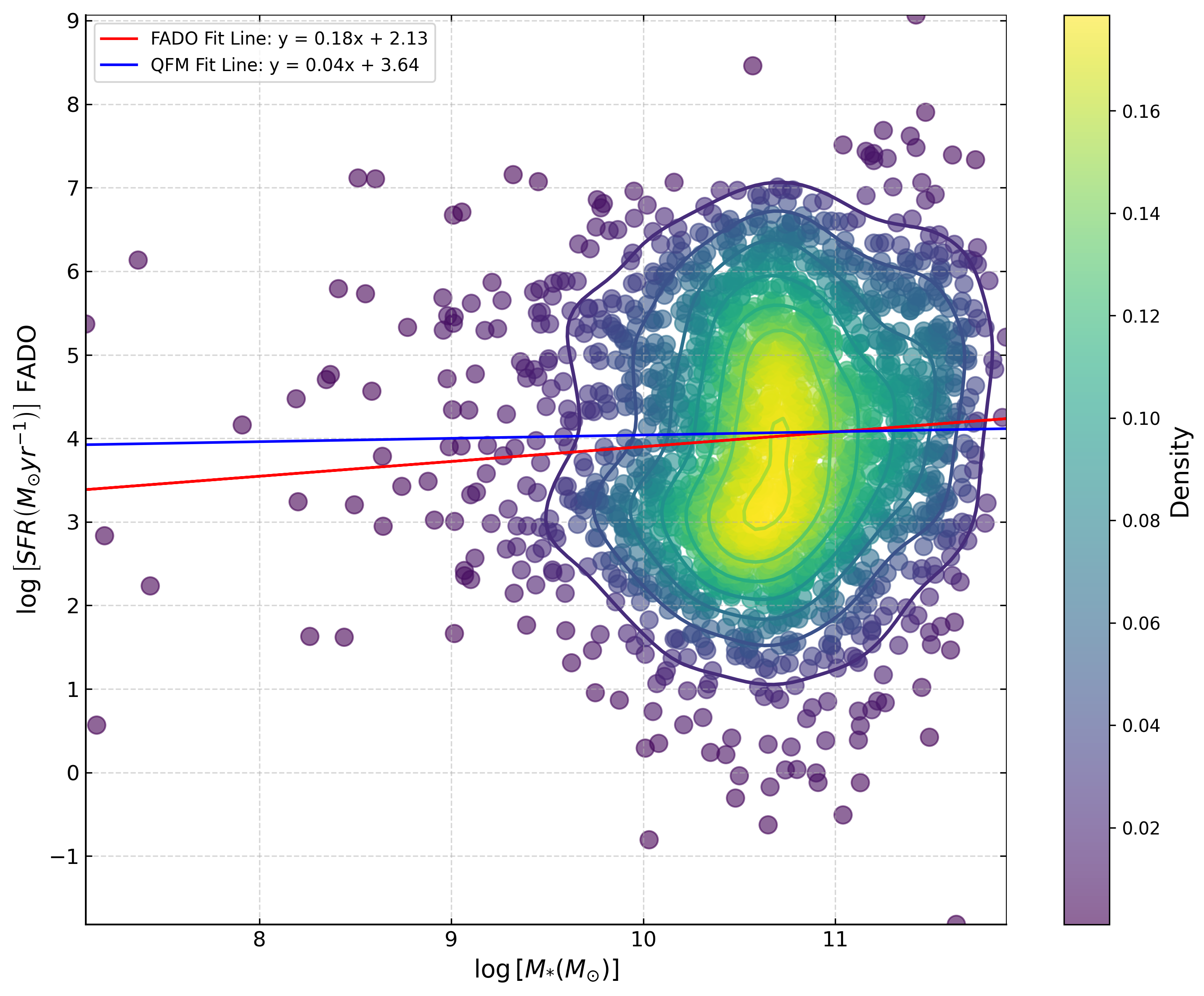
(a) FADO’s SFMS Figure

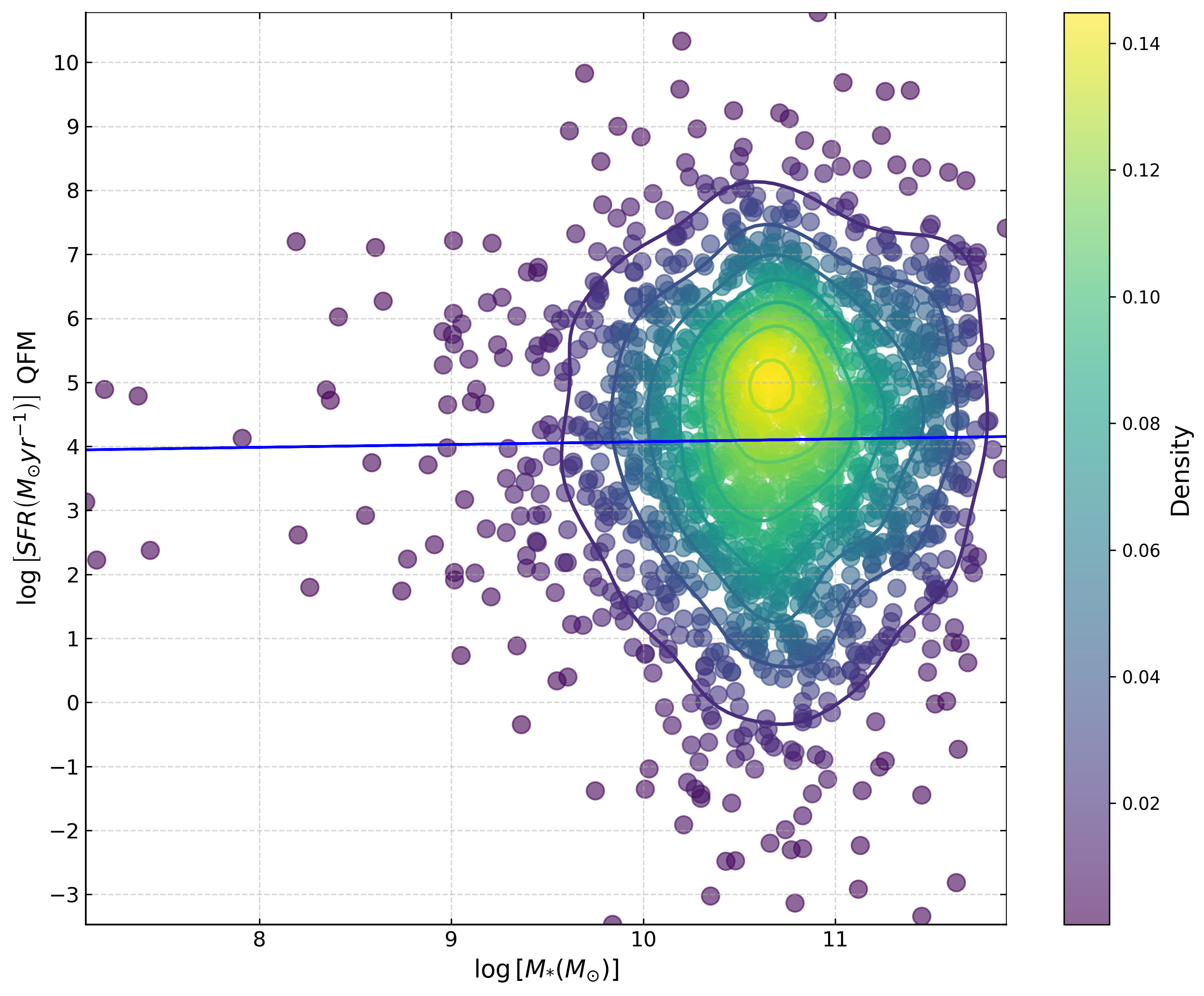
(b) QFM’s SFMS Figure

Figure 8: Left panel: SFMS diagram fitted by FADO. The red line represents the slope of the SFR calculated by FADO compared with the stellar mass, and the blue line represents the slope of the SFR calculated by qsofitmore compared with the stellar mass. The denser the data points, the brighter the area in the Figure, and vice versa. Right panel: SFMS diagram fitted by qsofitmore. The blue line represents the slope of the SFR calculated by qsofitmore compared with the stellar mass. The denser the data points, the brighter the area in the Figure, and vice versa.

Finally, we conclude that approximately 45$\%$ of the data points indicate that the H${\alpha}\lambda$6563 emission line fitted by FADO is smaller than that fitted by qsofitmore, which preliminarily suggests that FADO successfully subtracts some nebular emissions. Additionally, by examining the trend of the ratio between FADO fitting results and qsofitmore fitting results with redshift, we tentatively infer that nebular contamination increases with higher redshifts. Therefore, it is anticipated that when studying the SFR at high redshifts, the influence of nebular emissions should be removed.

4 discussions

In this section, we discuss four main issues, which will serve as a foundation for future research in this area. Firstly, we compare our results with the work of Miranda et al. (2023) to explain the significant differences between our main conclusions and the relevant parts of their work. Then, we attempt to identify other factors that could affect SFR estimation. In particular, we also discuss the impact of recent significant findings on the initial mass function on SFR estimation and its trend with redshift. Finally, we look forward to future joint analyses of higher-quality spectroscopic surveys and multi-band spectroscopy.

4.1 Comparison with Miranda’s results and uncertainty

In comparison to Miranda et al. (2023), who utilized the integrated MPA-JHU as the sample and obtained SFRs with slight or even negligible differences, this survey employed the latest comprehensive galaxy data from SDSS-DR18 and employed the BPT diagram to screen all data, ensuring that all data points are star-forming galaxies (SFGs). This guarantees that all data points exhibit significant differences in nebular contamination. Moreover, the redshift range used in this study, spanning from 0 to 0.5, exceeds the range of 0 to 0.25 used by Miranda et al. (2023). Although in the subsequent fitting process, galaxies with poor spectral quality in the redshift range of 0.4-0.5 were heavily excluded, this range represents the limit of accurately estimating SFR using H${\alpha}\lambda$6563 in the SDSS survey. In this survey, the redshift range of galaxies is extended to a maximum of 0.5, and preliminary evidence suggests that FADO effectively removes nebular radiation. Additionally, the presence of nebular contamination in SFR calculations increases with increasing redshift. The SFMS also indicates that SFRs derived by FADO align more closely with theoretical predictions. Due to significant errors associated with FADO, we plotted the Figures considering both with and without error scenarios, and the results reveal the anticipated trends under both circumstances. The following section will analyze the causes of large fitting errors.

Both FADO and qsofitmore employ the MC method to obtain uncertainties in emission lines, but there are still some dominant errors inherent in their respective codes. The large errors in FADO arise from its high degrees of freedom, and the error calculation method is relatively simple, involving the superposition of components. FADO fitting includes a greater variety of spectral fitting models and considers a wider range of components. As more statistical uncertainties and degeneracies are introduced among physical components, the comparison between the new code and the old code becomes increasingly complex (Cardoso et al., 2022). The uncertainties in FADO are also derived from random scattering in the MC model, with each step of FADO fitting generating an uncertainty caused by MC. Therefore, for FADO, a comprehensive and complex self-consistent code incorporating many spectral fitting scenarios inevitably generates more uncertainties. When these uncertainties are superimposed, it leads to significant errors observed in the Figures from the previous section. Moreover, there are significant variations in the fitted flux of H${\alpha}\lambda$6563, with results indicating that removing the flux of H${\alpha}\lambda$6563 from host galaxies and quasars better fits the trend line of Gaussian model fitting. The closer the variance value of the fitted data to the observed data is to 1, the closer the correlation between the two. Additionally, the number of random scattering points in MC still needs to be considered. FADO iterates the Monte Carlo algorithm more times, while for qsofitmore, we only iterated 15 times. More iterations bring uncertainties closer to reality, but excessive iterations exponentially increase the time taken for qsofitmore to process spectral fitting. To avoid lengthy spectral fitting times, we chose a relatively reasonable value. The greater number of iterations in FADO may be one of the reasons for the larger uncertainty associated with FADO.

4.2 Other factors affecting SFR estimation

The H${\alpha}\lambda$6563 line obtained by FADO is generally similar to that of qsofitmore, with a median ratio of $\sim$0.09, indicating that the pure stellar fitting model qsofitmore misinterprets a fraction of the nebular emissions as stellar formation activity. Although the overall discrepancy is small, Figure 6 demonstrates a clear trend, preliminarily suggesting an increase in the contribution of nebular emissions with increasing redshift. For the SED model used by FADO, factors such as electron density, extinction, temperature, and nebular kinematics influence the nebular term in the process of fitting spectra with FADO, with electron density and temperature being the dominant factors (Gomes & Papaderos, 2017). Therefore, the underestimation of SFR derived from FADO in this study may be partly attributed to the overestimation of electron density and temperature. Accurate estimation and constraints of galaxy SFR require the combination of multi-band spectral observations due to the distribution of ultraviolet, optical, and infrared radiations in different regions of galaxies and dust obscuration (Elbaz et al., 2018). Active Galactic Nuclei (AGNs) are considered to play a crucial role in shaping and evolving galaxies. The gas on the host galaxy disk interacts with AGN feedback, strongly influencing the overall galaxy SFR. AGNs that may exist in some starburst galaxies can trigger, enhance, or suppress star formation (Elbaz et al., 2018). This also affects the accuracy of estimating galaxy SFR, regardless of the spectral band used.

4.3 The impact of variable IMF on spectral fitting

Currently, models used for fitting galaxy spectra (e.g., FADO and qsofitmore) assume the initial mass function (IMF) of stars to be constant. However, various indications suggest that the IMF may not be a completely invariant cornerstone of spectral fitting theories. Li et al. (2023) recently announced that the IMF is a function primarily dependent on stellar metallicity rather than a constant as previously assumed. Since stellar metallicity varies among galaxies at different redshifts, the IMF becomes a function of redshift, and thus, future galaxy spectral fitting may need to consider the evolutionary trend of the IMF with redshift. This could profoundly affect the accurate estimation of galaxy SFRs and impose an additional redshift-evolution trend closely related to the IMF on the trend of SFR evolution with redshift.

The impact of IMF on this survey can be described as follows: (a) The luminosity of H${\alpha}\lambda$6563 is influenced by the IMF. The Lyman continuum (LyC) photon rate is strongly dependent on redshift, and the intensity of nebular emission lines remains a topic of ongoing debate due to inaccurate redshifts. If the Salpeter IMF is used, the luminosity of H${\alpha}\lambda$6563 will vary by a factor of 4.6 from z = 0.001 to z = 0.040 (Weilbacher & Fritze-v. Alvensleben, 2001). Therefore, calculating SFR using the luminosity of H${\alpha}\lambda$6563 can lead to significant errors. (b) The influence of metallicity on SFR. Low-metallicity stellar populations are brighter and hotter than solar-metallicity stellar populations with the same IMF and mass constraints. According to the survey by Weilbacher & Fritze-v. Alvensleben (2001), estimating the luminosity of H${\alpha}\lambda$6563 in low-metallicity dwarf galaxies using empirical calibration may result in an overestimation of the star formation rate by a factor of 3 due to the metallicity effect. (c) Metallicity affects the luminosity of H${\alpha}\lambda$6563, thereby affecting SFR: a comparison between the IMF of Scalo (1986) and Salpeter (1955) revealed a $35\%$ decrease in H${\alpha}\lambda$6563 luminosity (Gomes & Papaderos, 2017). (d) The impact of electron density (ne) on SFR. A drawback of all photoionization spectral synthesis (pss) codes is the neglect of ne, which is particularly crucial for modeling pss (Gomes & Papaderos, 2017). Higher electron density implies a higher probability of gas ionization, resulting in more ionized gas. Collisions between them lead to transitions in electron energy levels, ultimately affecting the estimation of SFR.

However, IMF remains an outstanding question in astrophysics to date. The variation in IMF seems not as straightforward as initially imagined. André et al. (2010)’s survey of nearby clouds indicates that the core mass function appears significantly steeper than the cloud mass function and is closer to the mass function of stars. Recently, Li et al. (2023) announced that the IMF is a primary function dependent on stellar metallicity rather than a constant function as previously believed. Since stellar metallicity varies among galaxies at different redshifts, the IMF becomes a function of redshift. Therefore, future galaxy spectral fitting may need to consider the evolutionary trend of the IMF with redshift. Generally, we cannot obtain the most accurate IMF, and we can only reduce the impact of IMF on SFR through other means, which FADO accomplishes reliably. Almost all of these calibrations are based on evolutionary synthesis models, where emerging SEDs are derived for composite stellar populations with specified age combinations, chemical compositions, and IMFs. The calibration by Kennicutt (1998) employs model combinations from the literature and assumes a single power-law IMF with mass limits of 0.1 and 100 $M_{\text{Sun}}$ (Salpeter, 1955). Compared to a more realistic IMF for H${\alpha}\lambda$6563, this IMF provides a satisfactory SFR calibration, but for other wavelengths, the relative calibration using different tracers is sensitive to the precise form of the IMF. Therefore, for this survey, we still adopt the IMF form of BC03 and H${\alpha}\lambda$6563 as the SFR tracer. Different IMFs will affect estimates of star formation rates and stellar mass. However, this effect can be directly addressed by applying a conversion factor between estimates obtained with two IMFs (Zahid et al., 2012).

4.4 Future spectroscopic data

This investigation ultimately obtained the expected results, demonstrating that SFR estimation of galaxies at higher redshifts is indeed affected by nebular emission. However, this investigation also has a limited sample size for SFR calculations. In addition to expecting improvements in the quality of future SDSS spectral data, supplementary studies using spectral surveys such as LAMOST and DESI have potential. Currently, the S/N of the spectra of the majority of SDSS galaxies with redshifts higher than 0.5 is very low, and the data quality is poor, making it difficult to identify and fit emission lines related to SFR estimation. Therefore, if exploring the SFR of galaxies at higher redshifts, especially those in the cosmic noon period at z $\sim$ 2, not only optical spectra but also UV or IR spectra need to be combined, which will require a huge amount of work. However, there are still doubts about whether FADO has good IR spectral analysis capabilities. We hope that the FADO team can improve and test the code of FADO in the future to perform well not only in IR but also in UV spectra. With the extensive implementation of galaxy IR observation projects by JWST, the era of large sample analysis of high-redshift galaxies will soon arrive. The question of the SFR of the first-generation galaxies in the universe will also be revealed.

In addition, it is imperative to mention that estimating the star formation rate (SFR) of a galaxy through multi-band observations leads to more precise results. The estimation of SFR via H${\alpha}$ emission is also constrained; H${\alpha}\lambda$6563 is mostly applicable to galaxies with mean ages ranging from 0.3 to 10 million years (Myr). Comparatively, utilizing 2-10 keV may yield more effective results than H${\alpha}\lambda$6563. Therefore, for accurate SFR computation, employing multi-band observations is essential to obtain the most comprehensive spectrum of the target galaxy, thereby deriving a complete SFR. Further weight is applied to alternative estimations of attenuation correction and SFR based on UV and IR measurements (Kennicutt & Evans, 2012). Additionally, disregarding the impact of the initial mass function (IMF), significant differences are evident in SFR calculations at H${\alpha}\lambda$6563 luminosities of $10^{38}$ (Cerviño et al., 2003). Neglecting the IMF effect for lower SFRs may result in the misestimation of stellar lifetimes, thereby elongating their lifecycle, and inducing larger fluctuations in H${\alpha}$ emission lines. Hence, employing tracers other than the H${\alpha}$ emission line to constrain SFR is advisable, such as FUV emission (Kennicutt & Evans, 2012). Observations in the infrared band are crucial for obtaining SFR, as interstellar dust absorbs half of the starlight in galaxies and re-emits it in the infrared. The morphological variations in different dust emission components translate into significant changes in the spectral energy distribution (SED) of dust within and between galaxies (Smith et al., 2007); thus, the conversion of SFR from multi-band observations still requires calibration based on different bands. In terms of correcting SFR after combining optical and infrared observations, Rosario et al. (2016); Kennicutt & Evans (2012) have made notable contributions.

Therefore, to obtain the most accurate SFR for galaxies, it is necessary to combine visible, infrared, and ultraviolet spectra of the target galaxy into a complete galaxy spectrum. However, the objective of this investigation is to compare the effects of two different fitting methods on SFR. Hence, the aforementioned impacts have fairly appeared in both fitting methods, canceling each other out. Nonetheless, it is crucial to note that obtaining accurate SFR requires the combination of correct IMF and multi-band observations.

5 summary

In this tentative work, we demonstrate that FADO, which considers the impact of nebular components on spectral fitting, gives a smaller SFR compared to the pure stellar model of qsofitmore. This further proves the viewpoint of Miranda et al. (2023) that the contribution of nebulae to SFR increases with higher redshift. This may provide some inspiration for later research on higher redshift SFR, where the contribution of nebulae cannot be ignored, especially for SBGs and SFGs. In the future, we expect to use a simultaneous analysis method of IR and optical spectra to obtain more obvious nebular radiation noise. The main conclusions of this study are presented below.

Firstly, about 45$\%$ of the data points indicate that qsofitmore underestimated the contribution of nebular emission, resulting in an overestimation of the calculated SFR. Secondly, as redshift increases, the contribution of nebular emission also increases, leading to a further increase in the difference between FADO and qsofitmore.Thirdly, the SFMS diagram shows that FADO’s data has values that are more consistent with theory, further illustrating the advantages of FADO for pure stellar codes. Finally, we predict that at higher redshifts, the difference in nebular emission between FADO and other pure stellar codes will be even greater.

Appendix A Intrinsic Extinction

Extinction generally refers to the process by which photons are absorbed, scattered, and reflected as they pass through a medium, thereby weakening in intensity. In astrophysics, photons from distant galaxies pass through the dust and gas of the galaxy itself, pass through the dust and gas of the Milky Way, and finally reach our telescopes. In order to obtain a more accurate emission line flux and thus calculate the SFR, the extinction of the galaxy itself is necessary. This extinction is called the intrinsic extinction of the galaxy. Follow the Cardelli, Clayton, and Mathis (1988, CCM) extinction definition from (Cardelli et al., 1989):

$$R_{V}=\frac{A_{V}}{E(B-V)}.$$ (A1)

Where $R_{V}$ is 3.1, standard value for the diffuse interstellar medium (ISM); $A_{V}$ represent the extinction at V-band; $E(B-V)$ represent colour excess.

$$\frac{A(\lambda)}{A_{V}}=a(\lambda)+\frac{b(\lambda)}{R_{V}},$$ (A2)

where $a(\lambda)$ and $b(\lambda)$ are the wavelength-dependent coefficients, which are polynomial of $\lambda$, in unit of $\mu m$ (see Eq. 3(a) and 3(b) in Cardelli et al., 1989). $A(\lambda)$ is absolute extinction as a function of wavelength. Substitute Equation A2 into Equation A1, and the rearranged equation can be:

$$\quad A(\lambda)=\left[\frac{a(\lambda)}{R_{V}}+b(\lambda)\right]\cdot E(B-V),$$ (A3)

Let $K(\lambda)=\frac{a(\lambda)}{R_{V}}+b(\lambda)$, the Equation A3 can be written as:

$$A(\lambda)=K(\lambda)\cdot E(B-V).$$ (A4)

Now, we need to consider the relationship between observed and intrinsic magnitude. Photons from distant galaxies pass through layers of dust and suffer from extinction effects. The intrinsic magnitude should be the difference between the observed magnitude and extinction value:

$$m_{\text{int}}=m_{\text{obs}}-A(\lambda),$$ (A5)

where $m_{\text{int}}$ represent intrinsic magnitude at wavelength of $\lambda$, while $m_{\text{obs}}$ the observed magnitude at wavelength of $\lambda$. Adopting the flux formula, the Equation A5 can be written as:

$$A(\lambda)=m_{\text{obs}}-m_{\text{int}}=-2.5\log\frac{F(\lambda)_{\text{obs}}}{F(\lambda)_{\text{int}}}.$$ (A6)

$F(\lambda)_{\text{obs}}$ is the main aim of this section, $F(\lambda)\text{ int }$ is the flux after extinction. To achieve this goal, we need to know $A(\lambda)$ and $F(\lambda)\text{ obs }$. $F(\lambda)\text{ obs }$ can easily get from spectrum. For $A(\lambda)$ can be found via Equation A4. The attenuation of dust on radiation varies in wavelength. Radiation with shorter wavelength suffers heavier attenuation, and vice versa. Therefore, $A(\lambda)$ can be calculated by comparing the observed fluxes of two different emission lines. We employ the flux ratio of $H_{\alpha}$ and $H_{\beta}$ to derive the corresponding $A(\lambda)$, which is the Balmer attenuation. Now for $H\alpha$ and $H\beta$:

$$H_{\alpha}:\quad m\alpha_{0}-m\alpha_{i}=A(H\alpha)=K(H\alpha)\cdot E(B-V),$$ (A7)

$$H\beta:\quad m\beta_{0}-m\beta_{i}=A(H\beta)=K(H\beta)\cdot E(B-V)\quad.$$ (A8)

Use Equation A7 - Equation A8 we can found:

$$m\alpha_{0}-m\alpha_{i}-\left(m\beta_{0}-m\beta_{i}\right)=[K(H\alpha)-K(H\beta)]\cdot E(B-V)\quad\text{}.$$ (A9)

Substitute Equation A6 into Equation A9, and rearrange equation can get:

$$E(B-V)=\frac{-2.5}{K(H\alpha)-K(H\beta)}\log\frac{(H\alpha/H\beta)_{\text{obs}}}{(H\alpha/H\beta)_{\text{int}}}.$$ (A10)

$K(H_{\alpha})$ and $K(H_{\beta})$ can be found via (Cardelli et al., 1989), ratio of $H\alpha$ and $H\beta$ have been given by FADO and QFM, $(H\alpha/H\beta)_{\text{int}}$ is 2.86 (Osterbrock, 1989). So, in this way, E(B-V) can be found. Finally, substitute Equation A10 into Equation A6, the $F(\lambda)_{\text{int}}$ can be found:

$$F(\lambda)_{\text{int}}=F(\lambda)_{\text{obs}}\ 10^{A(\lambda)/2.5}.$$ (A11)

Example of qsofitmore spectral fitting:

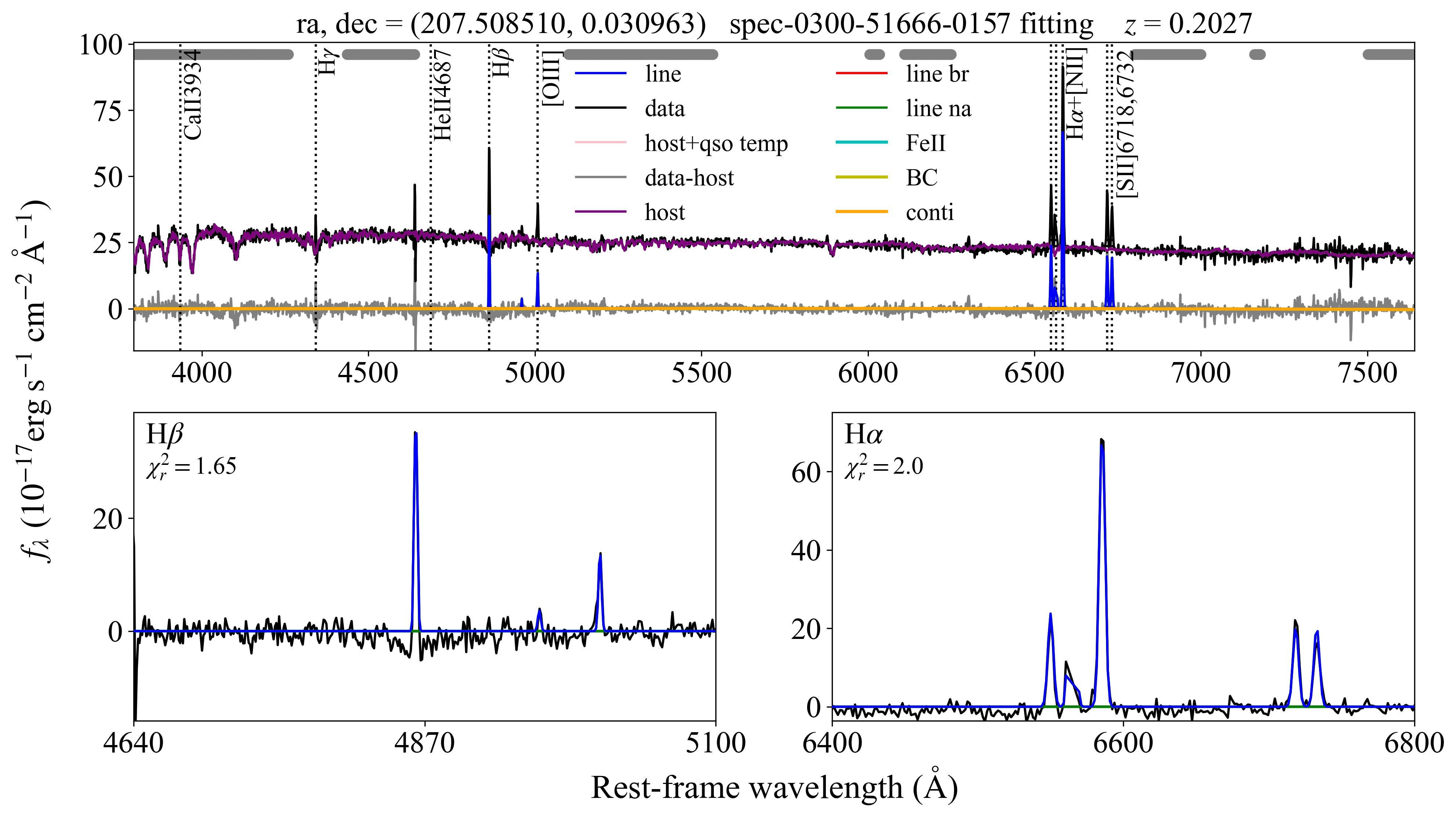
Figure 9: The fitting diagram of qsofitmore, the top panel shows the fitting of the whole band, and the following shows the fitting of $H\alpha$ and $H\beta$.

References

- Abazajian et al. (2009) Abazajian, K. N., Adelman-McCarthy, J. K., Agüeros, M. A., et al. 2009, ApJS, 182, 543, doi: 10.1088/0067-0049/182/2/543
- Ahumada et al. (2020) Ahumada, R., Allende Prieto, C., Almeida, A., et al. 2020, ApJS, 249, 3, doi: 10.3847/1538-4365/ab929e
- Almeida et al. (2023) Almeida, A., Anderson, S. F., Argudo-Fernández, M., et al. 2023, ApJS, 267, 44, doi: 10.3847/1538-4365/acda98
- André et al. (2010) André, P., Men’shchikov, A., Bontemps, S., et al. 2010, A&A, 518, L102, doi: 10.1051/0004-6361/201014666
- Baldwin et al. (1981) Baldwin, J. A., Phillips, M. M., & Terlevich, R. 1981, PASP, 93, 5, doi: 10.1086/130766
- Breda et al. (2022) Breda, I., Vilchez, J. M., Papaderos, P., et al. 2022, A&A, 663, A29, doi: 10.1051/0004-6361/202142805
- Bruzual & Charlot (2003) Bruzual, G., & Charlot, S. 2003, MNRAS, 344, 1000, doi: 10.1046/j.1365-8711.2003.06897.x
- Calzetti et al. (2000) Calzetti, D., Armus, L., Bohlin, R. C., et al. 2000, ApJ, 533, 682, doi: 10.1086/308692
- Cappellari & Emsellem (2004) Cappellari, M., & Emsellem, E. 2004, PASP, 116, 138, doi: 10.1086/381875
- Cardelli et al. (1989) Cardelli, J. A., Clayton, G. C., & Mathis, J. S. 1989, ApJ, 345, 245, doi: 10.1086/167900
- Cardoso et al. (2022) Cardoso, L. S. M., Gomes, J. M., Papaderos, P., et al. 2022, A&A, 667, A11, doi: 10.1051/0004-6361/202243856
- Cerviño et al. (2003) Cerviño, M., Luridiana, V., Pérez, E., Vílchez, J. M., & Valls-Gabaud, D. 2003, A&A, 407, 177, doi: 10.1051/0004-6361:20030861
- Chabrier (2003) Chabrier, G. 2003, ApJ, 586, L133, doi: 10.1086/374879
- Chen et al. (2024) Chen, G., Zheng, Z., Zeng, X., et al. 2024, ApJS, 271, 20, doi: 10.3847/1538-4365/ad1c67
- Cid Fernandes et al. (2005) Cid Fernandes, R., Mateus, A., Sodré, L., Stasińska, G., & Gomes, J. M. 2005, MNRAS, 358, 363, doi: 10.1111/j.1365-2966.2005.08752.x
- Daigne et al. (2004) Daigne, F., Olive, K. A., Vangioni-Flam, E., Silk, J., & Audouze, J. 2004, ApJ, 617, 693, doi: 10.1086/425649
- Di Matteo et al. (2005) Di Matteo, T., Springel, V., & Hernquist, L. 2005, Nature, 433, 604, doi: 10.1038/nature03335
- Ding et al. (2023) Ding, X., Onoue, M., Silverman, J. D., et al. 2023, Nature, 621, 51, doi: 10.1038/s41586-023-06345-5
- Elbaz et al. (2018) Elbaz, D., Leiton, R., Nagar, N., et al. 2018, A&A, 616, A110, doi: 10.1051/0004-6361/201732370
- Ellis et al. (2013) Ellis, R. S., McLure, R. J., Dunlop, J. S., et al. 2013, ApJ, 763, L7, doi: 10.1088/2041-8205/763/1/L7
- Förster Schreiber & Wuyts (2020) Förster Schreiber, N. M., & Wuyts, S. 2020, ARA&A, 58, 661, doi: 10.1146/annurev-astro-032620-021910
- Fu (2021) Fu, Y. 2021, QSOFITMORE: a python package for fitting UV-optical spectra of quasars, v1.1.0, Zenodo, Zenodo, doi: 10.5281/zenodo.5810042
- Fu et al. (2022) Fu, Y., Wu, X.-B., Jiang, L., et al. 2022, ApJS, 261, 32, doi: 10.3847/1538-4365/ac7f3e
- Gaskell & Ferland (1984) Gaskell, C. M., & Ferland, G. J. 1984, PASP, 96, 393, doi: 10.1086/131352
- Gomes & Papaderos (2017) Gomes, J. M., & Papaderos, P. 2017, A&A, 603, A63, doi: 10.1051/0004-6361/201628986
- Hummer & Storey (1987) Hummer, D. G., & Storey, P. J. 1987, MNRAS, 224, 801, doi: 10.1093/mnras/224.3.801
- Izotov et al. (2024) Izotov, Y. I., Schaerer, D., Guseva, N. G., Thuan, T. X., & Worseck, G. 2024, MNRAS, 528, L10, doi: 10.1093/mnrasl/slad166
- Jin et al. (2023) Jin, J.-J., Wu, X.-B., Fu, Y., et al. 2023, ApJS, 265, 25, doi: 10.3847/1538-4365/acaf89
- Kauffmann et al. (2003) Kauffmann, G., Heckman, T. M., Tremonti, C., et al. 2003, MNRAS, 346, 1055, doi: 10.1111/j.1365-2966.2003.07154.x
- Kennicutt (1998) Kennicutt, Robert C., J. 1998, ARA&A, 36, 189, doi: 10.1146/annurev.astro.36.1.189
- Kennicutt & Evans (2012) Kennicutt, R. C., & Evans, N. J. 2012, ARA&A, 50, 531, doi: 10.1146/annurev-astro-081811-125610
- Kewley et al. (2001) Kewley, L. J., Dopita, M. A., Sutherland, R. S., Heisler, C. A., & Trevena, J. 2001, ApJ, 556, 121, doi: 10.1086/321545
- Kewley et al. (2004) Kewley, L. J., Geller, M. J., & Jansen, R. A. 2004, AJ, 127, 2002, doi: 10.1086/382723
- Kirk et al. (2015) Kirk, H., Klassen, M., Pudritz, R., & Pillsworth, S. 2015, ApJ, 802, 75, doi: 10.1088/0004-637X/802/2/75
- Krueger et al. (1995) Krueger, H., Fritze-v. Alvensleben, U., & Loose, H. H. 1995, A&A, 303, 41
- Krumholz et al. (2012) Krumholz, M. R., Dekel, A., & McKee, C. F. 2012, ApJ, 745, 69, doi: 10.1088/0004-637X/745/1/69
- Lada & Lada (2003) Lada, C. J., & Lada, E. A. 2003, ARA&A, 41, 57, doi: 10.1146/annurev.astro.41.011802.094844
- Li et al. (2023) Li, J., Liu, C., Zhang, Z.-Y., et al. 2023, Nature, 613, 460, doi: 10.1038/s41586-022-05488-1
- Madau & Dickinson (2014) Madau, P., & Dickinson, M. 2014, ARA&A, 52, 415, doi: 10.1146/annurev-astro-081811-125615
- McKee & Ostriker (2007) McKee, C. F., & Ostriker, E. C. 2007, ARA&A, 45, 565, doi: 10.1146/annurev.astro.45.051806.110602
- McKee & Tan (2002) McKee, C. F., & Tan, J. C. 2002, Nature, 416, 59, doi: 10.1038/416059a
- Miranda et al. (2023) Miranda, H., Pappalardo, C., Papaderos, P., et al. 2023, A&A, 669, A16, doi: 10.1051/0004-6361/202244390
- Mullaney et al. (2012) Mullaney, J. R., Pannella, M., Daddi, E., et al. 2012, MNRAS, 419, 95, doi: 10.1111/j.1365-2966.2011.19675.x
- Noeske et al. (2007) Noeske, K. G., Weiner, B. J., Faber, S. M., et al. 2007, ApJ, 660, L43, doi: 10.1086/517926
- Osterbrock (1989) Osterbrock, D. E. 1989, Astrophysics of gaseous nebulae and active galactic nuclei
- Pacifici et al. (2015) Pacifici, C., da Cunha, E., Charlot, S., et al. 2015, MNRAS, 447, 786, doi: 10.1093/mnras/stu2447
- Pappalardo et al. (2021) Pappalardo, C., Cardoso, L. S. M., Michel Gomes, J., et al. 2021, A&A, 651, A99, doi: 10.1051/0004-6361/202039792
- Peng et al. (2010) Peng, Y.-j., Lilly, S. J., Kovač, K., et al. 2010, ApJ, 721, 193, doi: 10.1088/0004-637X/721/1/193
- Robertson & Ellis (2012) Robertson, B. E., & Ellis, R. S. 2012, ApJ, 744, 95, doi: 10.1088/0004-637X/744/2/95
- Rosario et al. (2016) Rosario, D. J., Mendel, J. T., Ellison, S. L., Lutz, D., & Trump, J. R. 2016, MNRAS, 457, 2703, doi: 10.1093/mnras/stw096
- Salim et al. (2007) Salim, S., Rich, R. M., Charlot, S., et al. 2007, ApJS, 173, 267, doi: 10.1086/519218
- Salpeter (1955) Salpeter, E. E. 1955, ApJ, 121, 161, doi: 10.1086/145971
- Schaerer & de Barros (2009) Schaerer, D., & de Barros, S. 2009, A&A, 502, 423, doi: 10.1051/0004-6361/200911781
- Scoville et al. (2023) Scoville, N., Faisst, A., Weaver, J., et al. 2023, ApJ, 943, 82, doi: 10.3847/1538-4357/aca1bc
- Shapley et al. (2023) Shapley, A. E., Reddy, N. A., Sanders, R. L., Topping, M. W., & Brammer, G. B. 2023, ApJ, 950, L1, doi: 10.3847/2041-8213/acd939
- Smith et al. (2007) Smith, J. D. T., Draine, B. T., Dale, D. A., et al. 2007, ApJ, 656, 770, doi: 10.1086/510549
- Sobral et al. (2013) Sobral, D., Smail, I., Best, P. N., et al. 2013, MNRAS, 428, 1128, doi: 10.1093/mnras/sts096
- Springel et al. (2005) Springel, V., Di Matteo, T., & Hernquist, L. 2005, MNRAS, 361, 776, doi: 10.1111/j.1365-2966.2005.09238.x
- Tacconi et al. (2020) Tacconi, L. J., Genzel, R., & Sternberg, A. 2020, ARA&A, 58, 157, doi: 10.1146/annurev-astro-082812-141034
- Wang (2013) Wang, F. Y. 2013, A&A, 556, A90, doi: 10.1051/0004-6361/201321623
- Wang et al. (2013) Wang, R., Wagg, J., Carilli, C. L., et al. 2013, ApJ, 773, 44, doi: 10.1088/0004-637X/773/1/44
- Weilbacher & Fritze-v. Alvensleben (2001) Weilbacher, P. M., & Fritze-v. Alvensleben, U. 2001, A&A, 373, L9, doi: 10.1051/0004-6361:20010704
- Zahid et al. (2012) Zahid, H. J., Dima, G. I., Kewley, L. J., Erb, D. K., & Davé, R. 2012, ApJ, 757, 54, doi: 10.1088/0004-637X/757/1/54
- Zhuang & Ho (2019) Zhuang, M.-Y., & Ho, L. C. 2019, ApJ, 882, 89, doi: 10.3847/1538-4357/ab340d