A twist for nonlocal thermoelectricity in quantum wires as a signature of Bogoliubov-Fermi points
Juan Herrera Mateos
ECyT-ICIFI Universidad Nacional de San Martín, Campus Miguelete, 25 de Mayo y Francia, 1650 Buenos Aires, Argentina
Leandro Tosi
Grupo de Circuitos Cuánticos, Div. Dispositivos y Sensores, Centro Atómico Bariloche (8400), San Carlos de Bariloche, Argentina
Alessandro Braggio
NEST, Istituto Nanoscienze-CNR and Scuola Normale Superiore, I-56126 Pisa, Italy
Fabio Taddei
NEST, Istituto Nanoscienze-CNR and Scuola Normale Superiore, I-56126 Pisa, Italy
Liliana Arrachea
ECyT-ICIFI Universidad Nacional de San Martín, Campus Miguelete, 25 de Mayo y Francia, 1650 Buenos Aires, Argentina
ECyT-ICIFI, Universidad Nacional de San Martín, Campus Miguelete, 25 de Mayo y Francia, 1650 Buenos Aires, Argentina
Grupo de Circuitos Cuánticos, Div. Dispositivos y Sensores, Centro Atómico Bariloche (8400), San Carlos de Bariloche, Argentina
Istituto Nanoscienze-CNR and NEST Scuola Normale Superiore, I-56127 Pisa, Italy
Istituto Nanoscienze-CNR and NEST Scuola Normale Superiore, I-56127 Pisa, Italy
ECyT-ICIFI, Universidad Nacional de San Martín, Campus Miguelete, 25 de Mayo y Francia, 1650 Buenos Aires, Argentina
Abstract
We study nonlocal thermoelectricity in a superconducting wire subject to spin-orbit coupling and a magnetic field with a relative orientation between them. We calculate the current flowing in a normal probe attached to the bulk of a superconducting wire, as a result of a temperature difference applied at the ends of the wire.
We find that the thermoelectric response occurs in ranges of the angles which correspond to the emergence of
Bogoliubov Fermi points in the energy spectrum of the superconducting wire.
Introduction.
The concept of achieving a topological phase featuring Majorana zero modes [1, 2] was the driving force for numerous theoretical and experimental studies
into superconducting InAs wires [3, 4, 5, 6, 7, 8, 9, 10, 11]. The appealing features of these systems rely on three crucial ingredients: resilient induced superconductivity, strong spin-orbit coupling (SOC)
and large gyromagnetic factor.
An equally fascinating phenomenon is the emergence of Bogoliubov-Fermi surfaces, whose signatures have been
recently observed in InAs two-dimensional systems with an applied in-plane magnetic field proximitized by superconductors [12]. The energetic stability and the topological properties of this peculiar phase have been the motivation of several theoretical studies [13, 14, 15, 16, 17].
In this Letter, we show that the emergence of Bogoliubov Fermi points in a superconducting wire with SOC and magnetic field can lead to a nonlocal thermoelectric response.
These wires exhibit a topological phase across a range of chemical potentials (), pairing amplitudes () and Zeeman energies ()
subject to the condition that the angle () between the directions of the SOC and
the magnetic field satisfies [18, 19, 20, 21, 22].
Bogoliubov Fermi points emerge as the gap in the spectrum of the topological phase is partially closed by a twist beyond the critical angles defined by this condition.
This nonlocal thermoelectric response bears similarities to that
recently proposed to take place in Josephson junctions of two-dimensional topological insulators
[23, 24, 25].
In that case, it is induced by a Doppler shift generated by a magnetic flux threading the junction [26].
Here, the pivotal role is played by the twist of the magnetic field giving rise to the Bogoliubov Fermi points.
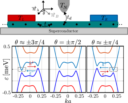
Figure 1: Top: Sketch of the setup. Bottom: Spectrum of the Bogoliubov-de-Gennes Hamiltonian describing the wires with , , , and
, for different values of the angle between the direction of the SOC and the magnetic field. For the spectrum is fully gapped with two cones symmetrically aligned to . For () the cone with () crosses zero energy, defining
Bogoliubov Fermi points with right-moving electrons and left-moving holes (right-moving electrons and left-moving holes). These states account for the nonlocal thermoelectric response.
Model. We consider the setup sketched in Fig. 1(a), where a quantum wire is proximitized with local s-wave superconductivity and has SOC and magnetic field acting in the directions and , respectively, with . A temperature difference () is imposed between the left () and the right () portions of the wire. A third terminal consisting of a normal-metal probe (N) is contacted at some point along the length of the wire with a
tunnel-coupling . The nonlocal thermoelectric effect corresponds to an electrical current generated at the normal probe as a response to the transversal thermal bias.
The wire is described by the Hamiltonian
, which is expressed in the Nambu basis and the Bogoliubov-de-Gennes (BdG) Hamiltonian matrix is given by [1, 2]
(1)
The Pauli matrices and act in the spin and particle-hole degrees of freedom, respectively, while are the 22 unitary matrices. is the kinetic dispersion relation relative to the chemical potential , being the nearest-neighbor hopping and is the lattice constant. The SOC is described by , while is the Zeeman splitting due to the magnetic field and is the local s-wave pairing potential.
In the results shown hereafter, we consider parameters of this Hamiltonian that are representative of reported experimental research in InAs wires [4, 5]. We assign , which fits the continuum model for the wires for
. We consider for the SOC, for the pairing potential
and a g-factor , which corresponds to a Zeeman splitting energy for a magnetic field .
The eigenspectrum corresponding to the Hamiltonian of Eq. (1) is shown in the bottom panel of Fig. 1 for different values of . We can identify two bands generated by the Zeeman splitting, which are doubled in the BdG representation. When the magnetic field is perpendicular to the SOC () the spectrum is fully gaped for all values of . Due to the combination of the SOC and , the effective pairing has s-wave as well as p-wave components [1, 2, 27, 28]. The latter is the dominant one when the system is in the topological phase for .
This is precisely the situation illustrated in the figure.
When the orientation of the magnetic field is twisted, such that overcomes the critical values defined by the condition ,
the superconducting gap is partially closed. In fact, the “cones” of the spectrum cross zero energy from positive (negative) energies defining Bogoliubov-Fermi points for ().
The right (left) bottom panels of Fig. 1 correspond to .
In what follows, we argue that the scenario of Bogoliubov-Fermi points illustrated in Fig. 1 hosts the fundamental ingredients to have a nonlocal thermoelectric response. It is well known that a necessary condition for the phenomenon of thermoelectricity to take place is the transmission probabilities not to be even in energy
[29]. This condition usually relies on the implementation of energy filters in two-terminal configurations and is difficult to realize in superconductors since these systems are intrinsically particle-hole symmetric [30, 31, 32, 33, 34, 35, 36, 37, 38, 39].
In fact, we see that the three spectra shown in Fig. 1 have this symmetry. The key ingredient for nonlocal thermoelectricity in the setup we are studying is to generate an imbalance between left-moving electrons (thermalized with the right reservoir) and right-moving holes (thermalized with the left reservoir). Hence, as a consequence of an applied temperature difference at the superconducting reservoirs, the fluxes associated with the two types of quasiparticles into the normal probe are not compensated and a net current is generated. In the spectrum of Fig. 1 with the low-energy cone with () corresponds to a right-moving electron (hole) and a left-moving hole (electron). Importantly, the spectrum is symmetrical to , implying identical velocities and density of states of the left and right movers. In the twisted case, we can identify a low-energy branch of Bogoliubons forming Fermi points with electrons moving to the right and holes moving to the left (see plots with ). The opposite situation takes place for . This mechanism may display a thermoelectric response since it produces the necessary particle-hole imbalance. In what follows, we show explicit calculations of the thermoelectric current that confirm this picture. Before, it is interesting to compare with the situation discussed in Ref. [23] for a device where the Kramers pair of helical edge states of a topological insulator in a Josephson junction.
In that case, the imbalance between electrons and holes was induced by a Doppler shift generated by the magnetic flux threading the junction. Although different, both systems share common features. In fact, in both cases, the low-energy spectrum hosts a pair of
left-right movers with different spin orientations in contact with a s-wave superconductor. Because of the broken
SU(2) symmetry, in both systems superconducting pairing is induced in both s-wave and p-wave channels. The effect of the twisted magnetic field in our case and the Doppler shift in the case of Ref. [23] is to introduce an asymmetry in the spectrum so that a single pair of particle-hole quasiparticles moving in opposite directions dominate the quantum energy transport.
Thermoelectric current. We focus on the linear-response regime and introduce the formal description of the nonlocal thermoelectric effect in this framework. We consider and for the left and right terminals of the wire, respectively, and for the normal probe. We consider that the reservoirs connected to the ends of the wire are grounded (), while we consider the possibility of an electrical bias at the normal terminal. We define affinities and and assume they are small enough to justify treating them in the linear response. The induced charge current at the normal lead reads
.
The Onsager coefficients are
(2)
where . The functions and are, respectively, the transmission probabilities for an electron-like and hole-like quasiparticle starting from the superconducting lead to go in lead , while is the Andreev reflection probability for an electron starting from lead to be reflected as a hole. The Fermi function is evaluated at the base temperature . The derivative of this function entering the coefficients of Eq. (A twist for nonlocal thermoelectricity in quantum wires as a signature of Bogoliubov-Fermi points) defines the relevant transport window .
In addition, notice that is a local quantity, which corresponds to the convergence of the transport channels between the two superconducting terminals into the one. Instead is a nonlocal quantity, corresponding to the difference in the thermoelectrical transport between the and terminals and the one and we have stressed this property with the label “nl”. The possibility of having a local thermoelectric response in this setup is discussed in the supplementary material (see Ref [40]). We also present there the details of the derivation of Eqs. (A twist for nonlocal thermoelectricity in quantum wires as a signature of Bogoliubov-Fermi points) and the expressions for the transmission functions, , and the Andreev reflection function, in terms of non-equilibrium Green’s functions. These functions satisfy
which implies a change of sign of at .
The relevant transport coefficients we discuss next are the conductance and the nonlocal Seebeck coefficient . These are defined from the Onsager parameters as
(3)
Numerical Results. In the calculations
the reservoirs at the temperatures and are modeled by the same Hamiltonian
and parameters as the wire with a recursive method [41]. Details are presented in Ref. [40].
In linear response, the results do not depend on the length of the central wire but depend on the tunnelling coupling between the normal probe and the wire.
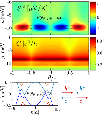
Figure 2: and as functions of and for the same parameters of the wire as in Fig. 1. Other parameters are
and . The topological phase is within the rectangles indicated in dashed lines. Bottom panel: spectrum corresponding to the point for which the nonlocal thermoelectric response is weak.
In Fig. 2 we present the resulting conductance and Seebeck coefficient as functions of the chemical potential and relative SOC-magnetic field angle . We can identify in the top panel of the figure, regions where the Seebeck coefficient takes large positive and negative values.
These are the nonlocal thermoelectric features anticipated from the analysis of the spectrum with Bologiubov Fermi points. In fact, notice that the value of corresponding to the spectrum of Fig. 1 is precisely the one for which the largest values of are achieved. We can, in particular, verify the vanishing nonlocal thermoelectric response for for which the spectrum is symmetric with respect to . In addition, the opposite signs of for given angles and are consistent with the interchange of right-moving particle-like and left-moving hole-like quasiparticles observed in the spectra of Fig. 1 and also with the symmetry properties of the functions . In the bottom panel of Fig. 2 we show, for comparison the spectrum for the parameters indicated in the top panel where the thermoelectric response is weaker, albeit non-vanishing.
For the dominant superconducting pairing is an s-wave type and four quasiparticle cones emerge at low energy in the spectrum (two for and two for ). For , four Bogoliubov-Fermi points emerge at each side of . Focusing at , we can identify an electron-hole cone crossing zero energy from above along with a hole-electron cone crossing zero energy from below. The nature of these low-energy quasiparticles is consistent with a pair of left-moving electrons and right-moving holes partially compensated by a pair of right-moving electrons and left-moving holes. Consequently, there is a partial cancellation of the nonlocal thermoelectric transport. In conclusion, the nonlocal thermoelectrical effect is much stronger when a single Bogoliubov-Fermi cone is present.
This is precisely the case of emerging Fermi points within the topological phase.
The behavior of the conductance is affected by the density of states of the wire and also to the coupling between wire and the normal probe.
It achieves a maximum close to , just above the boundary for the topological phase. This is because the density of states of the wire is large for this value of and the two spin channels contribute to the transport.
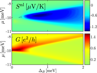
Figure 3: and as functions of and for . Other parameters are the same as the previous Figs.
The topological phase is inside the small triangle highlighted in a dashed line in the upper panel.
It is defined by and (vertical gray line).
A complementary and helpful perspective can be obtained by fixing the angle and changing the magnetic field. In Fig. 3 we focus on and show again and as functions of and . In the behavior of these quantities we can identify the gap (see blue region in the upper panel), within which is minimal while the nonlocal thermoelectric response is strongest.
The small triangle with dashed line in the upper panel of this Fig. defines the boundary for the topological phase. As in the previous figure we see that the
maximal response in is associated to the emergence of the Bogoliubov Fermi points. Such an effect occurs as the magnetic field is twisted beyond the critical value defined by . From the experimental point of view, it is important to notice
that remains close to the maximal values across a wide range of and , which facilitates the exploration of this effect by varying the magnetic field.
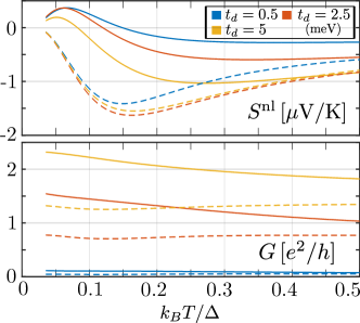
Figure 4: and as functions of temperature for the same parameters as the previous Figs. and different values of coupling with the normal reservoir, .
Solid (dashed) lines correspond to ().
Finally, in Fig. 4 we show and obtained for different couplings between the normal probe and the wire, as a function of the temperature .
We focus on low enough , so that we can neglect dependence of on .
The amplitude of the non-local Seebeck coefficient
decreases as a function of the temperature. This is consistent with the fact that, for increasing temperature, high-energy regions of the spectrum play a role. Such excitations
contain electrons and holes traveling in opposite directions, with the concomitant suppression of the non-local thermoelectric response. This behavior thermoelectric is anomalous. It strongly differs from the standard behavior of the Seebeck coefficient which typically scales with the temperature. The effect of temperature is clearly weaker in the conductance. In addition, the thermoelectric response is not strongly affected by the coupling , while the opposite is true regarding the conductance.
Summary and Conclusions. We have shown the existence of a nonlocal thermoelectric response in a superconducting wire hosting spin-orbit interaction with twisted orientations of a magnetic field with respect to the wire SOC main axis. We predict this effect to take place in systems akin to those typically used in the search for Majorana zero modes [3, 4, 5, 6, 7].
The possible impact of these modes in thermoelectric effects has been explored in structures with quantum dots [42, 43, 44, 45, 46, 47, 48, 49, 50, 51, 52].
In contrast, the non-local effect here addressed is related to the emergence of Bogoliubov Fermi points. This takes place when the gap of the topological phase is partially closed by a twist of the magnetic field with respect to the SOC, beyond a critical alignment and has been recently observed in two-dimensional samples of these materials [12]. The estimate of the Seebeck coefficient, albeit small, is compatible with measured thermovoltages in other systems [53, 54, 55], assuming temperature differences of mK. Its behaviour is strongly sensitive to the relative orientation of the magnetic field and the SOC, providing a valuable hallmark of this fundamental property.
Acknowledgements.
L.T. acknowledges the Georg Forster Fellowship from the Humboldt Stiftung. L.A., L.T. and J.H.M. thank
support from CONICET as well as FonCyT, Argentina, through grants PICT-2018-04536 and PICT 2020-A-03661. L.A. would also like to thank the Institut Henri Poincaré (UAR 839 CNRS-Sorbonne Université) and the LabEx CARMIN (ANR-10-LABX-59-01) for their support. A.B. and F.T. acknowledge the MUR-PRIN 2022 - Grant No. 2022B9P8LN - (PE3)-Project NEThEQS ”Non-equilibrium coherent thermal effects in quantum systems” in PNRR Mission 4 - Component 2 - Investment 1.1 ”Fondo per il Programma Nazionale di Ricerca e Progetti di Rilevante Interesse Nazionale (PRIN)” funded by the European Union - Next Generation EU and the Royal Society through the International Exchanges between the UK and Italy (Grants No. IEC R2 192166).
A.B. acknowledges EU’s Horizon 2020 Research and Innovation Framework Programme Grant No. 964398 (SUPERGATE) and No. 101057977 (SPECTRUM), and CNR project QTHERMONANO.
References
Lutchyn et al. [2010]R. M. Lutchyn, J. D. Sau, and S. D. Sarma, Majorana fermions and a topological phase transition in semiconductor-superconductor heterostructures, Physical Review Letters 105, 077001 (2010).
Mourik et al. [2012]V. Mourik, K. Zuo, S. M. Frolov, S. Plissard, E. P. Bakkers, and L. P. Kouwenhoven, Signatures of majorana fermions in hybrid superconductor-semiconductor nanowire devices, Science 336, 1003 (2012).
Deng et al. [2016]M. Deng, S. Vaitiekėnas, E. B. Hansen, J. Danon, M. Leijnse, K. Flensberg, J. Nygård, P. Krogstrup, and C. M. Marcus, Majorana bound state in a coupled quantum-dot hybrid-nanowire system, Science 354, 1557 (2016).
Chen et al. [2017]J. Chen, P. Yu, J. Stenger, M. Hocevar, D. Car, S. R. Plissard, E. P. Bakkers, T. D. Stanescu, and S. M. Frolov, Experimental phase diagram of zero-bias conductance peaks in superconductor/semiconductor nanowire devices, Science Advances 3, e1701476 (2017).
Chen et al. [2019]J. Chen, B. D. Woods, P. Yu, M. Hocevar, D. Car, S. R. Plissard, E. P. A. M. Bakkers, T. D. Stanescu, and S. M. Frolov, Ubiquitous non-majorana zero-bias conductance peaks in nanowire devices, Physical Review Letters 123, 107703 (2019).
Nichele et al. [2017]F. Nichele, A. C. Drachmann, A. M. Whiticar, E. C. O’Farrell, H. J. Suominen, A. Fornieri, T. Wang, G. C. Gardner, C. Thomas, and A. T. Hatke, Scaling of majorana zero-bias conductance peaks, Physical Review Letters 119, 136803 (2017).
Vaitiekenas et al. [2020]S. Vaitiekenas, G. W. Winkler, B. van Heck, T. Karzig, M.-T. Deng, K. Flensberg, L. I. Glazman, C. Nayak, P. Krogstrup, R. M. Lutchyn, and C. M. Marcus, Flux-induced topological superconductivity in full-shell nanowires, Science 367, eaav3392
(2020).
Alicea [2012]J. Alicea, New directions in the pursuit of majorana fermions in solid state systems, Reports on progress in physics 75, 076501 (2012).
Prada et al. [2020]E. Prada, P. San-Jose, M. W. de Moor, A. Geresdi, E. J. Lee, J. Klinovaja, D. Loss, J. Nygård, R. Aguado, and L. P. Kouwenhoven, From andreev to majorana bound states in hybrid superconductor–semiconductor nanowires, Nature Reviews Physics 2, 575 (2020).
Flensberg et al. [2021]K. Flensberg, F. von Oppen, and A. Stern, Engineered platforms for topological superconductivity and majorana zero modes, Nature Reviews Materials 6, 944 (2021).
Phan et al. [2022]D. Phan, J. Senior, A. Ghazaryan, M. Hatefipour, W. Strickland, J. Shabani, M. Serbyn, and A. P. Higginbotham, Detecting induced pi p pairing at the al-inas interface with a quantum microwave circuit, Physical Review Letters 128, 107701 (2022).
Liu and Wilczek [2003]W. V. Liu and F. Wilczek, Interior gap superfluidity, Physical Review Letters 90, 047002 (2003).
Wu and Yip [2003]S.-T. Wu and S. Yip, Superfluidity in the interior-gap states, Physical Review A 67, 053603 (2003).
Forbes et al. [2005]M. M. Forbes, E. Gubankova, W. V. Liu, and F. Wilczek, Stability criteria for breached-pair superfluidity, Physical Review Letters 94, 017001 (2005).
Agterberg et al. [2017]D. F. Agterberg, P. M. R. Brydon, and C. Timm, Bogoliubov Fermi Surfaces in Superconductors with Broken Time-Reversal Symmetry, Physical Review Letters 118, 127001 (2017).
Setty et al. [2020]C. Setty, Y. Cao, A. Kreisel, S. Bhattacharyya, and P. Hirschfeld, Bogoliubov fermi surfaces in spin-1 2 systems: Model hamiltonians and experimental consequences, Physical Review B 102, 064504 (2020).
Rex and Sudbø [2014]S. Rex and A. Sudbø, Tilting of the magnetic field in majorana nanowires: Critical angle and zero-energy differential conductance, Physical Review B 90, 115429 (2014).
Osca et al. [2014]J. Osca, D. Ruiz, and L. Serra, Effects of tilting the magnetic field in one-dimensional majorana nanowires, Physical Review B 89, 245405 (2014).
Klinovaja and Loss [2015]J. Klinovaja and D. Loss, Fermionic and majorana bound states in hybrid nanowires with non-uniform spin-orbit interaction, The European Physical Journal B 88, 1 (2015).
Aligia et al. [2020a]A. A. Aligia, D. P. Daroca, and L. Arrachea, Tomography of zero-energy end modes in topological superconducting wires, Physical Review Letters 125, 256801 (2020a).
Daroca and Aligia [2021]D. P. Daroca and A. A. Aligia, Phase diagram of a model for topological superconducting wires, Physical Review B 104, 115125 (2021).
Blasi et al. [2020a]G. Blasi, F. Taddei, L. Arrachea, M. Carrega, and A. Braggio, Nonlocal thermoelectricity in a superconductor–topological-insulator-superconductor junction in contact with a normal-metal probe: Evidence for helical edge states, Physical Review Letters 124, 227701 (2020a).
Blasi et al. [2020b]G. Blasi, F. Taddei, L. Arrachea, M. Carrega, and A. Braggio, Nonlocal thermoelectricity in a topological andreev interferometer, Physical Review B 102, 241302 (2020b).
Blasi et al. [2021]G. Blasi, F. Taddei, L. Arrachea, M. Carrega, and A. Braggio, Nonlocal thermoelectric engines in hybrid topological josephson junctions, Physical Review B 103, 235434 (2021).
Tkachov et al. [2015]G. Tkachov, P. Burset, B. Trauzettel, and E. M. Hankiewicz, Quantum interference of edge supercurrents in a two-dimensional topological insulator, Physical Review B 92, 045408 (2015).
Aligia et al. [2020b]A. A. Aligia, D. Pérez Daroca, and L. Arrachea, Tomography of zero-energy end modes in topological superconducting wires, Physical Review Letters 125, 256801 (2020b).
Gruñeiro et al. [2023]L. Gruñeiro, M. Alvarado, A. L. Yeyati, and L. Arrachea, Transport features of a topological superconducting nanowire with a quantum dot: Conductance and noise, Physical Review B 108, 045418 (2023).
Benenti et al. [2017]G. Benenti, G. Casati, K. Saito, and R. S. Whitney, Fundamental aspects of steady-state conversion of heat to work at the nanoscale, Physics Reports 694, 1 (2017).
Ozaeta et al. [2014]A. Ozaeta, P. Virtanen, F. Bergeret, and T. Heikkilä, Predicted very large thermoelectric effect in ferromagnet-superconductor junctions in the presence of a spin-splitting magnetic field, Physical Review Letters 112, 057001 (2014).
Kolenda et al. [2017]S. Kolenda, C. Sürgers, G. Fischer, and D. Beckmann, Thermoelectric effects in superconductor-ferromagnet tunnel junctions on europium sulfide, Physical Review B 95, 224505 (2017).
Shapiro et al. [2017]D. S. Shapiro, D. Feldman, A. D. Mirlin, and A. Shnirman, Thermoelectric transport in junctions of majorana and dirac channels, Physical Review B 95, 195425 (2017).
Keidel et al. [2020]F. Keidel, S.-Y. Hwang, B. Trauzettel, B. Sothmann, and P. Burset, On-demand thermoelectric generation of equal-spin cooper pairs, Physical Review Research 2, 022019 (2020).
Mukhopadhyay and Das [2022]A. Mukhopadhyay and S. Das, Thermal bias induced charge current in a josephson junction: From ballistic to disordered, Physical Review B 106, 075421 (2022).
Machon et al. [2013]P. Machon, M. Eschrig, and W. Belzig, Nonlocal thermoelectric effects and nonlocal onsager relations in a three-terminal proximity-coupled superconductor-ferromagnet device, Physical Review Letters 110, 047002 (2013).
Mazza et al. [2015]F. Mazza, S. Valentini, R. Bosisio, G. Benenti, V. Giovannetti, R. Fazio, and F. Taddei, Separation of heat and charge currents for boosted thermoelectric conversion, Physical Review B 91, 245435 (2015).
Heidrich and Beckmann [2019]J. Heidrich and D. Beckmann, Nonlocal thermoelectric effects in high-field superconductor-ferromagnet hybrid structures, Physical Review B 100, 134501 (2019).
Braggio et al. [2024]A. Braggio, M. Carrega, B. Sothmann, and R. Sánchez, Nonlocal thermoelectric detection of interaction and correlations in edge states, Physical Review Research 6, L012049 (2024).
Tabatabaei et al. [2022]S. M. Tabatabaei, D. Sánchez, A. L. Yeyati, and R. Sánchez, Nonlocal quantum heat engines made of hybrid superconducting devices, Physical Review B 106, 115419 (2022).
[40]See supplementary material.
Sancho et al. [1985]M. P. L. Sancho, J. M. L. Sancho, and J. Rubio, Highly convergent schemes for the calculation of bulk and surface green functions, J. Phys. F: Met Phys. 15, 851 (1985).
Lopez et al. [2014]R. Lopez, M. Lee, L. Serra, and J. S. Lim, Thermoelectrical detection of majorana states, Physical Review B 89, 205418 (2014).
Valentini et al. [2015]S. Valentini, R. Fazio, V. Giovannetti, and F. Taddei, Thermopower of three-terminal topological superconducting systems, Physical Review B 91, 045430 (2015).
Chi et al. [2020]F. Chi, Z.-G. Fu, J. Liu, K.-M. Li, Z. Wang, and P. Zhang, Thermoelectric Effect in a Correlated Quantum Dot Side-Coupled to Majorana Bound States, Nanoscale Res. Lett. 15, 1 (2020).
Hou et al. [2013]C.-Y. Hou, K. Shtengel, and G. Refael, Thermopower and Mott formula for a Majorana edge state, Physical Review B 88, 075304 (2013).
Ramos-Andrade et al. [2016]J. P. Ramos-Andrade, O. Ávalos Ovando, P. A. Orellana, and S. E. Ulloa, Thermoelectric transport through Majorana bound states and violation of Wiedemann-Franz law, Physical Review B 94, 155436 (2016).
Majek et al. [2022]P. Majek, K. P. Wójcik, and I. Weymann, Spin-resolved thermal signatures of Majorana-Kondo interplay in double quantum dots, Physical Review B 105, 075418 (2022).
Buccheri et al. [2022]F. Buccheri, A. Nava, R. Egger, P. Sodano, and D. Giuliano, Violation of the Wiedemann-Franz law in the topological Kondo model, Physical Review B 105, L081403 (2022).
Wang et al. [2019]X.-Q. Wang, S.-F. Zhang, Y. Han, G.-Y. Yi, and W.-J. Gong, Efficient enhancement of the thermoelectric effect due to the Majorana zero modes coupled to one quantum-dot system, Physical Review B 99, 195424 (2019).
Klees et al. [2023]R. L. Klees, D. Gresta, J. Sturm, L. W. Molenkamp, and E. M. Hankiewicz, Majorana-mediated thermoelectric transport in multiterminal junctions, arXiv 10.48550/arXiv.2306.17845 (2023), 2306.17845 .
Molenkamp et al. [1990]L. W. Molenkamp, H. van Houten, C. W. J. Beenakker, R. Eppenga, and C. T. Foxon, Quantum oscillations in the transverse voltage of a channel in the nonlinear transport regime, Physical Review Letters 65, 1052 (1990).
Dutta et al. [2019]B. Dutta, D. Majidi, A. García Corral, P. A. Erdman, S. Florens, T. A. Costi, H. Courtois, and C. B. Winkelmann, Direct Probe of the Seebeck Coefficient in a Kondo-Correlated Single-Quantum-Dot Transistor, Nano Letters 19, 506 (2019).
Real et al. [2020]M. Real, D. Gresta, C. Reichl, J. Weis, A. Tonina, P. Giudici, L. Arrachea, W. Wegscheider, and W. Dietsche, Thermoelectricity in quantum hall corbino structures, Physical Review Applied 14, 034019 (2020).
Suplementary material for: “A twist for nonlocal thermoelectricity in quantum wires as a signature of Bogoliubov Fermi points”
Suplementary material for: “A twist for nonlocal thermoelectricity in quantum wires as a signature of Bogoliubov Fermi points”
We present here technical details on the calculation of the current in terms of non-equilibrium Green’s functions. We also discuss the behavior of the transmission functions and the Andreev reflection.
I Nonlocal tunneling current
We calculate the expression for the current in terms of non-equilibrium Green’s function formalism.
We consider a wire modeled by the lattice Hamiltonian defined in the main text. In the present calculation we consider a wire of finite size
containing lattice sites with a lattice constant (). The wire is contacted to left () and right () superconducting reservoirs
represented by semi-infinite wires of a superconductor described by the same lattice Hamiltonian as the central wire. These reservoirs have
temperatures
and , respectively. A site (labeled by ) of the central wire is connected to a normal reservoir, which is modelled by a tight-binding Hamiltonian. For convenience, we consider a intermediate single lattice site (or quantum dot), which defines an interface between
the wire and the normal lead.
The full Hamiltonian reads
(4)
where the Hamiltonian for the superconducting wire expressed in real space and connected to a semi-infinite BCS Hamiltonian with singlet pairing reads
(5)
with .
For reservoirs described by a Hamiltonian with the same parameters of the wire, we can omit the subscript in the parameters , ,
, and .
We work in the coordinate system where the -axis is oriented along the wire and the -axis is oriented along the SOC. We consider in the plane. The sites representing the reservoirs are (left reservoir) and (right reservoir).
The Hamiltonian for the normal contact is a 1D tight binding Hamiltonian with hopping ,
(6)
where we are using the notation for the Nambu spinor within the normal lead. This system is assumed to
be at temperature and voltage .
The interface is modeled by
(7)
being the Nambu spinor that describes the degrees of freedom in the quantum dot.
is the magnetic field and
is a local energy representing a barrier, which can be controlled by an external gate voltage, in which case, the intermediate site plays the role of a non-interacting quantum dot.
The last term of Eq. (4) is the tunneling-contact between the quantum dot and the S and N leads. It reads
(8)
where the label denotes the sites of the wire and normal chains that are tunnel-coupled to the interface, respectively. Notice
that for and the quantum dot is assimilated to the normal lead.
The current flowing between the quantum dot and the normal lead reads
(9)
where . We have introduced the
lesser Green’s function
(10)
as well as the Fourier transform .
The equations to calculate the retarded Green’s functions and their properties are presented in Section III.
Using Eqs. (III.2) we can rewrite the argument of Eq. (9) as follows
(11)
Using properties of the Green’s functions –see Eq. (III.2)– we can write,
Calculating the sum over the elements of these matrices, we notice that
and . Hence, the current can be expressed as follows,
(15)
where the first term describes the normal transmission
and reads
(16)
(17)
while the second term of Eq. (15) describes the Andreev reflection and reads,
(18)
where the contributions of elements 1 and 2, and 3 and 4 are equal.
II Linear response
II.1 Onsager coefficients
We focus on the linear-response regime. We consider the general case where
(19)
The chemical potentials are , while we consider the possibility of an electrical bias at the normal terminal.
Expanding the differences of Fermi functions up to first order in the bias voltage, we have: and . Similarly, expanding the Fermi functions up to the first order in the temperature differences we have,
, where for , while for
and . The result is
(20)
being and . The Onsager coefficients read
(21)
II.2 Properties of the transmission functions.
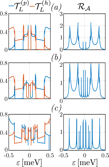
The behavior of the particle and hole transmission functions defined in Eqs. (16) and (17) are illustrated in Fig. 5 for the left reservoir, along with the Andreev reflection for the same parameters. The functions corresponding to the other reservoir exhibit similar features.
Figure 5: Transmisions and Andreev reflection functions for a system with , , , , and: (a) , ; (b) , or (c) , .
We can verify that these functions satisfy:
(22)
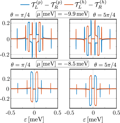
In Fig. 6 we show the difference of the transmission functions associated to the and superconductors.
This combination of transmission functions determine the non-local thermoelectric response and illustrate the
symmetry properties above mentioned.
Figure 6: Difference in transmission functions involved in the calculation of for a system with , , , and .
II.3 Non-local vs local thermoelectric response.
According to what was mentioned, depending on how symmetrical the temperature difference between the superconducting reservoirs is, we have a non-local, local thermoelectric response or a combination of both.
Given the temperatures as defined in Eq. (19), we see that the thermoelectric response is purely nonlocal when the temperature bias at the superconducting wire is perfectly symmetric with respect to the reference temperature of the normal probe, which corresponds to . In the opposite limit, where , the temperature bias is completely asymmetric, since only one of the terminals of the wire is thermally bias with respect to the normal probe, and in this limit, only the local component contributes. Intermediate
situations correspond to and the two components contribute.
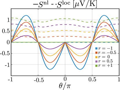
The behavior of the local and non-local components of the Seebeck coefficient defined as
are shown in Fig. 7 as functions of for different values of the factor .
We see the high sensitivity of the non-local thermoelectric effect to the , in contrast with the local one, which depends mildly on this angle.
This Fig. highlights the importance of implementing a symmetric temperature bias (), in order to cleanly observe the non-local thermoelectric effect.
Figure 7: non-local and local Seebeck coefficient as function of , for a sistem with , , , , , , for different values of , the factor that quantifies the asymmetry of temperatures between the superconducting reservoirs L and R. corresponds to the purely non-local case and to the purely local case.
III Calculation of Green’s functions
We present here the Dyson’s equations leading to the calculation of the retarded Green’s functions.
III.1 Retarded/Advanced
The Dyson equation for the
retarded Green’s function reads
(23)
Substituting the first equation in the second one we get
(24)
where we have introduce the definition of the retarded Green’s function of the quantum dot isolated from the rest of the subsystems,
(25)
the self-energies
(26)
as well as
the Green’s function of the wire connected to the two superconducting reservoirs but disconnected from the quantum dot and the normal lead,
evaluated at the connecting site . It reads
(27)
being the Green’s function of the free wire (notice that this is a matrix), while
are the self-energies describing the coupling of the wire to the superconducting leads . These can be also represented as
matrices with non-vanishing submatrices associated to the spacial coordinates
(for ) and (for ), respectively.
The non-vanishing self-energy matrices read
(28)
with is the matrix element representing the contact between the wire and the reservoirs. This contains the hopping as well as
the spin-orbit terms and is the Green’s function for the semi-infinite superconducting wire representing the reservoir. This is calculated by means of a recursive algorithm [41].
The self-energy describing the contact to the normal lead reads ,
being the Green’s function of the normal lead, which is also calculated by a recursive algorithm.
The advanced functions can be calculated from
(29)
III.2 Lesser
The lesser Green’s functions can be calculated from the retarded/advanced ones by recourse to Langreth’s rule.
In particular,
(30)
The different self-energies are
(31)
being
(32)
with and
(35)
We have introduced the Fermi functions
and ,
being the inverse temperature of the reservoir .
Notice that only the normal lead is biased with a voltage .
Substituting we get
(36)
being
(37)
III.3 Identities
The following identity can be shown
(38)
Another important identity can be derived by noticing that the current defined in Eq. (9) should be zero in equilibrium.
This implies
(39)
Substituting the definitions of all these quantities we get
(40)
where is the Fermi-Dirac distribution function corresponding to the equilibrium system. Since this function is a common factor in all the terms,
this identity is zero for any argument of .