EKF–SINDy: Empowering the extended Kalman filter with sparse identification of nonlinear dynamics

Abstract

Observed data from a dynamic system can be assimilated into a predictive model by means of Kalman filters. Nonlinear extensions of the Kalman filter, such as the Extended Kalman Filter (EKF), are required to enable the joint estimation of (possibly nonlinear) system dynamics and of input parameters. To construct the evolution model used in the prediction phase of the EKF, we propose to rely on the Sparse Identification of Nonlinear Dynamics (SINDy). The numerical integration of a SINDy model leads to great computational savings compared to alternate strategies based on, e.g., finite elements. Indeed, SINDy allows for the immediate definition of the Jacobian matrices required by the EKF to identify system dynamics and properties, a derivation that is usually extremely involved with physical models. As a result, combining the EKF with SINDy provides a computationally efficient, easy-to-apply approach for the identification of nonlinear systems, capable of robust operation even outside the range of training of SINDy. To demonstrate the potential of the approach, we address the identification of a linear non-autonomous system consisting of a shear building model excited by real seismograms, and the identification of a partially observed nonlinear system. The challenge arising from applying SINDy when the system state is not accessible has been relieved by means of time-delay embedding. The great accuracy and the small uncertainty associated with the state identification, where the state has been augmented to include system properties, underscores the great potential of the proposed strategy, paving the way for the development of predictive digital twins in different fields.

1 Introduction

Dynamic system identification is crucial to enable the construction of predictive digital twins [1], and to implement control strategies for engineering systems with applications to condition-based maintenance of civil structures [2], or to fuel consumption reduction in air transportation [3]. Despite advances in Machine Learning (ML) and Data Science [4], identifying explainable, reduced dimensional models of dynamic processes from big data is an open field of research [5]. Searching for the physical relations that underlie a certain dynamic process is probably the best way to obtain robust and generalisable models, a characteristic uncommon in most of ML techniques. Consequently, making reliable predictions in scenarios lacking collected data is generally challenging or impossible [6]. This type of uncertainty is commonly referred to as epistemic uncertainty. To address this challenge, we employ the Sparse Identification of Nonlinear Dynamics (SINDy) proposed in [5]. SINDy constructs robust and generalisable models by assuming that only a few important terms govern the dynamics of the considered system. This assumption holds for many physical systems when an appropriate basis is used to describe the space of functions governing their dynamics [5].

To construct a digital twin, the model must evolve over time to reflect potential changes in its physical counterpart. This evolution should be, possibly online, driven by real-world data [7]. In this work, we have exploited an Extended Kalman filters (EKF) to perform data assimilation [8] leveraging a prediction-correction scheme. During the prediction stage, the SINDy model evolves the system state. The procedure can also accommodate potential external forcing rendering the system not autonomous. During the correction stage, acquired data are used to refine previous estimates, update the physical parameters governing the system dynamics, and potentially reduce the associated uncertainties. As a result, a joint estimation of the system is achieved (termed joint because both the state of the system and the physical parameters underlying the dynamics are jointly updated, see [9]). A schematic representation of the EKF-SINDy procedure is reported in Fig. 1. More details on this methodology will be discussed in Sec. 2.

In realistic applications, the observation variables assimilated by the EKF do not necessarily match up with the system state on which SINDy is performed. This mismatch arises in two scenarios: where the observations are fewer than the system state variables, potentially limiting the full description of the system dynamics, and where observations are in excess, potentially overwhelming the EKF-SINDy framework with redundant information. In the former case, we can resort to uplifting techniques such as, e.g., embedding techniques [10, 11] or recurrent decoder networks [12], to recover the hidden state components from the available, observed time-series. To address the latter case, dimensionality reduction techniques, employing proper orthogonal decomposition and/or encoder neural networks, have been coupled with SINDy to simultaneously reduce dimensionality while learning the corresponding governing dynamical system as in [13, 11, 14]. In this work, we deal with the first scenario, focusing on revealing hidden variables when only partial observations are available. The integration in the method of dimensionality reduction techniques to deal with high-dimensional data will be the focus of future work.

Figure 1: EKF-SINDy methodology. In the prediction phase, the dynamical system identified by SINDy advances the augmented state $\boldsymbol{\varkappa}=[\mathbf{x}^{\top},\boldsymbol{\phi}^{\top}]^{\top}$—comprising system state $\mathbf{x}$ and parameters $\boldsymbol{\phi}$—to a prior estimate $\boldsymbol{\varkappa}^{-}$; the correction phase involves the EKF assimilating system observations $\bar{\mathbf{y}}$, resulting in the updated augmented state $\boldsymbol{\varkappa}^{+}$.

In the recent literature, other works employ a ML-based identified model in the prediction phase of the KF. In [15], predictions were made using recurrent Neural Networks (NN), specifically Long Short-Term Memory (LSTM) modules; LSTM modules were also utilised to model the process and observation noise required by the filter. The linear KF was used to estimate only the dynamics of the observed system. In contrast, our work explicitly calibrates the physical parameters affecting the dynamical process, like in [16] where NNs and EKF were combined to perform joint estimation of mechanical systems. This work improved upon previously proposed variational autoencoders-based approaches, such as the deep Markov models [17], by relying on the EKF equation to infer the latent variables governing the system dynamics. Compared to [16], our methodology looks better suited for a physical process whose dynamics is controlled by a few important terms. This is because NNs require large volume of training data, do not easily account for known symmetries and constraints, and struggle to handle epistemic uncertainties [18].

SINDy has previously been coupled with the KF in [19]. In that work, the estimation procedure directly targeted the SINDy coefficients. However, as previously mentioned, relying on the linear KF precludes the possibility of performing joint estimation. At variance with [15], the proposal of [19] focused on identifying the coefficients of dynamic models without correcting the state predictions.

The application of the proposed approach to experimental data appears to be extremely promising. SINDy can be directly identified from preliminary acquired data. In this study, we have tested our methodology using simulated data for two primary reasons: first, to showcase the method potential and its ability to handle non autonomous and partially observed nonlinear systems; moreover, to demonstrate that the proposed methodology may be advantageous even when a physics-based model of the system is available. In the latter case, the model identified by SINDy serves as a surrogate for the physics-based model enabling significant computational time savings compared to the integration of nonlinear models. Relying on fast computational approaches has recently proven crucial in many applications, such as the design optimisation of Micro-Electro Mechanical Systems (MEMS) [20], and inverse analysis in structural health monitoring [21, 22], just to mention two relevant cases dealing with structural dynamics, both at the micro- and the macro-scale. The need of computational efficiency also underlies the use of SINDy in control applications [18, 23]. Alternatively, a recent work proposed to reduce the computational burden of the estimation process by using a rank-reduced version of the KF [24]. Another major advantage of using SINDy is the greatly simplified computation of the Jacobian matrices required by the EKF formulation, compared to the involved derivation typically encountered even for relatively simple mechanical systems [25].

The remainder of the paper is organized as follows. The methodology is presented in Sec. 2: first, KF is introduced; then the rationale behind SINDy is discussed; finally, the application of EKF-SINDy to joint estimation of autonomous and non-autonomous dynamic systems is detailed. Two case studies are presented in Sec. 3. In Sec. 3.1, a first case discusses the identification of a shear building subjected to a seismic event. Real seismograms are used as excitations, demonstrating the capability of our procedure of handling non-autonomous systems. A second case study, presented in Sec. 3.2, focuses on the identification of a partially observed nonlinear resonator. To address the impossibility to observe the whole system state, we precede the training of the SINDy model by applying the time-delay embedding [26]. Final considerations are collected in Sec. 4, along with a discussion of future developments. The source code of the proposed method is made available in the public repository EKF-SINDy [27].

2 Methodology

2.1 Extended Kalman Filtering

Considering a dynamic system of interest, Kalman filters exploit a state–space representation of the type:

$$\dot{\mathbf{x}}(t)=\frac{\text{d}}{\text{d}t}\mathbf{x}(t)=\mathbf{f}(\mathbf{x}(t)),$$ (1)

where: $\mathbf{x}(t)\in\mathbb{R}^{n}$ is the state vector of the system at time $t$; $\mathbf{f}:\mathbb{R}^{n}\rightarrow\mathbb{R}^{n}$ is the function of $\mathbf{x}(t)$ describing the dynamics of the system. Nonlinear versions of the KF, like the EKF, are required if $\mathbf{f}$ is nonlinear. Hereon, we rely on the extended Kalman filter (EKF); the reader may refer, e.g., to [28] for a complete derivation and analysis of the EKF theory.

Dynamic systems can be used to model the response of a building to seismic excitations, or the behavior of MEMS [29]. In general, $\mathbf{f}$ is not exactly known. Thus, it becomes important to assimilate incoming data of the system to update the model and the resulting predictions. For instance, these data can consist of floor acceleration measurements for a building [30], or displacement measurements for capacitive sensors. According to the discrete acquisition of system measurements, data assimilation is performed at discrete $t_{j}$ instants of observation, with $j=1,\ldots,T$. As state variables may not be directly compared against incoming data, the following observation equation:

$$\mathbf{y}(t_{j})=\mathbf{h}(\mathbf{x}(t_{j})),$$ (2)

s usually introduced to encode the state-to-observation map. Specifically: $\mathbf{h}:\mathbb{R}^{n}\rightarrow\mathbb{R}^{o}$ is a possibly nonlinear function; $\mathbf{y}(t_{j})\in\mathbb{R}^{o}$ are the quantities to be compared with the incoming observations $\bar{\mathbf{y}}(t_{j})\in\mathbb{R}^{o}$. According to Eqs. (1) and (2), model predictions are performed employing a continuous time description, while data assimilation is carried out at discrete time steps. For this reason, a hybrid (continuous–discrete) formulation of the KF will be considered in the following.

A prediction–correction scheme is then adopted to perform data assimilation. In the prediction phase, the state of the system is advanced in time through $\mathbf{f}$. This prediction is then corrected online through the comparison with incoming data. Hereon, we will use the superscript “$-$” to refer to quantities not yet updated by the correction stage, and the superscript “$+$” for quantities updated by the correction stage.

To perform the prediction–correction scheme, state variables are treated as random variables. Therefore, Eqs. (1) and (2) are modified as follows:

$$\dot{\mathbf{x}}(t) =\mathbf{f}(\mathbf{x}(t))+\mathbf{q}_{x},$$ (3a)

$$\mathbf{y}(t) =\mathbf{h}(\mathbf{x}(t))+\mathbf{r},$$ (3b)

where: $\mathbf{q}_{x}$ is the process noise vector, assumed to be sampled from a white, zero mean stochastic process $\mathbf{q}_{x}\sim\mathcal{N}(\mathbf{0},\mathbf{Q}_{x})$ with diagonal covariance matrix $\mathbf{Q}_{x}\in\mathbb{R}^{n\times n}$; $\mathbf{r}\in\mathbb{R}^{o}$ is the observation noise vector, assumed to be sampled from a white, zero-mean stochastic process $\mathbf{r}\sim\mathcal{N}(\mathbf{0},\mathbf{R})$ with diagonal covariance matrix $\mathbf{R}\in\mathbb{R}^{o\times o}$. The vector $\mathbf{q}_{x}$ accounts for uncertainties in the mapping $\mathbf{f}$, while $\mathbf{r}_{x}$ accounts for the noise affecting the incoming data. Their trade-off determines how much the filter relies on model predictions with respect to the acquired data [31].

The Kalman filter follows the system evolution by looking at $\hat{\mathbf{x}}$ and $\mathbf{P}$, where: $\hat{\mathbf{x}}=\mathbb{E}[\mathbf{x}]$ is the mean value of $\mathbf{x}$; $\mathbb{E}$ computes the expected value of a quantity; $\mathbf{P}=\mathbb{E}[(\mathbf{x}-\hat{\mathbf{x}})(\mathbf{x}-\hat{\mathbf{x}})^{\top}]$ is the covariance matrix associated to $\mathbf{x}$.

Prediction stage

The values of $\hat{\mathbf{x}}^{-}(t_{j})$ and $\mathbf{P}^{-}(t_{j})$ at $t_{j}$ are predicted starting from $\hat{\mathbf{x}}^{+}(t_{j\!-\!1})$ and $\mathbf{P}^{+}(t_{j\!-\!1})$ at $t_{j\!-\!1}$. These values have been obtained by correcting the previous estimates with data acquired at $t_{j-1}$. The prediction at $t_{j}$ is performed as in the following:

$$\hat{\mathbf{x}}^{-}(t_{j})=\hat{\mathbf{x}}^{+}(t_{j\!-\!1})+\int_{t_{j-1}}^{t_{j}}\mathbf{f}(\hat{\mathbf{x}}^{-}(\tau))\text{d}\tau,$$ (4a)

$$\mathbf{P}^{-}(t_{j})=\mathbf{P}^{+}(t_{j-1})+\int_{t_{j\!-\!1}}^{t_{j}}\mathbf{F}^{-}(\tau)\mathbf{P}^{-}(\tau)+\mathbf{P}^{-}(\tau)\mathbf{F}^{-}(\tau)^{\top}+\mathbf{Q}_{x}\text{ }\text{d}\tau,$$ (4b)

where $\mathbf{F}$ is the Jacobian of $\mathbf{f}(\mathbf{x}(t))$. The matrix $\mathbf{F}^{-}(\tau)$ is evaluated as:

$$\mathbf{F}^{-}(\tau)=\frac{\partial\mathbf{f}}{\partial\mathbf{x}^{\top}}\bigg{|}_{\hat{\mathbf{x}}^{-}(\tau)}.$$ (5)

Different methods can be used to integrate Eq. (4). For its computational efficiency, we have considered the Euler forward method leading to:

$$\hat{\mathbf{x}}^{-}(t_{j})=\hat{\mathbf{x}}^{+}(t_{j\!-\!1})+\Delta t~{}\mathbf{f}(\hat{\mathbf{x}}^{+}(t_{j\!-\!1})),$$ (6a)

$$\mathbf{P}^{-}(t_{j})=\mathbf{P}^{+}(t_{j\!-\!1})+\Delta t\left(\mathbf{F}^{+}(t_{j\!-\!1})\mathbf{P}^{+}(t_{j\!-\!1})+\mathbf{P}^{+}(t_{j\!-\!1})\mathbf{F}^{+^{\top}}(t_{j\!-\!1})+\mathbf{Q}_{x}\right),$$ (6b)

where $\mathbf{F}^{+}_{j-1}$ is evaluated for $\hat{\mathbf{x}}^{+}_{j-1}$ at $t_{j-1}$. In general, $\mathbf{Q}_{x}$ may modify in time; however, we neglect such possibility in this work. Moreover, we assume a constant time sampling $\Delta t=t_{j}-t_{j\!-\!1}$.

The Euler forward method is here a first-order explicit time integration technique, meaning that the local truncation error generated scales linearly with the time step $\Delta t$, provided this latter is chosen to be sufficiently small. More accurate methods can be employed, such as, e.g., higher-order Runge–Kutta methods. However, in the next section we will show that the local truncation error performed by the Euler forward method does not preclude good outcomes for the system estimation, also thanks to the adopted prediction–correction strategy. Similarly, implicit time stepping schemes can also be considered in order not to strongly constrain the choice of the time step, but it implies the solution of a (non)linear system of equations at each time step, in the case of (non)linear dynamic systems.

Correction stage

Once the prediction stage is accomplished, the correction stage is performed by assimilating the incoming data. Specifically, KF performs corrections in order to minimise the trace of $\mathbf{P}$. In the EKF, the following equations are enforced:

$$\mathbf{G}(t_{j})=\mathbf{P}^{-}(t_{j}){\mathbf{H}^{-}(t_{j})}^{\top}(\mathbf{H}^{-}(t_{j})\mathbf{P}^{-}(t_{j}){\mathbf{H}^{-}(t_{j})}^{\top}\!\!+\mathbf{R})^{-1},$$ (7a)

$$\hat{\mathbf{x}}^{+}(t_{j})=\hat{\mathbf{x}}^{-}(t_{j})+\mathbf{G}(t_{j})(\bar{\mathbf{y}}(t_{j})-\mathbf{h}(\hat{\mathbf{x}}^{-}(t_{j}),t_{j})),$$ (7b)

$$\mathbf{P}^{+}\!(t_{j})\!=\!\left(\mathbf{I}\!-\!\mathbf{G}(t_{j})\mathbf{H}^{-}(t_{j})\right)\mathbf{P}^{-}(t_{j})\left(\mathbf{I}\!-\!\mathbf{G}(t_{j})\mathbf{H}^{-}(t_{j})\right)^{\top}\!\!\!+\!\mathbf{G}(t_{j})\mathbf{R}\mathbf{G}(t_{j})^{\top},$$ (7c)

where: $\mathbf{G}(t_{j})$ is the Kalman gain matrix at $t_{j}$; $\mathbf{H}$ is the Jacobian of $\mathbf{h}$. The matrix $\mathbf{H}^{-}(t_{j})$ is evaluated for $\mathbf{x}^{-}(t_{j})$ as in the following:

$$\mathbf{H}^{-}(t_{j})=\frac{\partial\mathbf{h}}{\partial\mathbf{x}^{\top}}\bigg{|}_{\hat{\mathbf{x}}^{-}(t_{j})}.$$ (8)

When the KF is used to predict and correct the estimate of a set of variables describing the system dynamics, it is said that the procedure performs state estimation. The procedure can be extended to perform joint estimation as we will discuss in Sec. 2.3. As noted in the Introduction, the dimensionality of the observations ${\mathbf{y}}\in\mathbb{R}^{o}$ does not necessarily coincide with the dimensionality of the system state $\mathbf{x}\in\mathbb{R}^{n}$, thus potentially leading to $o\neq n$.

2.2 State estimation of autonomous dynamical system

The mapping $\mathbf{f}$ is only sometimes known, but, even if this is the case, the computation of $\mathbf{F}$ can be rather involved, while its numerical calculation can be computationally expensive. These reasons suggest to use SINDy to replace $\mathbf{f}$. Indeed, by expressing $\mathbf{f}$ as the linear combination of a set of predetermined functions collected in a library, as SINDy does, its (partial) derivatives can be simply obtained by combining the (partial) derivatives of the library functions. Analogously, even though $\mathbf{h}$ does not describe a dynamic system, it could be also identified using SINDy, thus greatly simplifying the computation of $\mathbf{H}$. However, in general the function $\mathbf{h}$ is directly set by means of more straightforward techniques. In the first case study proposed in this work, system state and observations represent the same dynamic quantities, and they do not require a distinct identification for $\mathbf{h}$. In the second case study, $\mathbf{h}$ has been determined from the time-delay embedding required by SINDy to (fully) learn $\mathbf{f}$.

For sake of generality, we now consider to use SINDy to model both $\mathbf{f}$ and $\mathbf{h}$. A detailed procedure is reported for $\mathbf{f}$, but the same strategy can also be applied to $\mathbf{h}$. The discussion is related to autonomous systems, i.e., systems without external forcing; in the next section, this assumption will be relaxed to allow for non-autonomous systems.

To apply the SINDy technique, it is first necessary to collect snapshots of the state vector to define the following matrix:

$$\mathbf{X}=\begin{bmatrix}\mathbf{x}^{\top}(t_{1})\\ \mathbf{x}^{\top}(t_{2})\\ \vdots\\ \mathbf{x}^{\top}(t_{T})\end{bmatrix}=\begin{bmatrix}x_{1}(t_{1})&x_{2}(t_{1})&\cdots&x_{n}(t_{1})\\ x_{1}(t_{2})&x_{2}(t_{2})&\cdots&x_{n}(t_{2})\\ \vdots&\vdots&\ddots&\vdots\\ x_{1}(t_{T})&x_{2}(t_{T})&\cdots&x_{n}(t_{T})\end{bmatrix}.$$ (9)

where $x_{i}(t_{j})$ is the i-th entry of $\mathbf{x}$ at the $j$-th time instant.

Similarly, a matrix $\dot{\mathbf{X}}$ is constructed by collecting the time derivatives $\dot{\mathbf{x}}$. We remark that the number of snapshots should not be necessarily equal to $T$. If $\mathbf{f}$ is available, Eq. (1) can be used to generate $\mathbf{X}$ and $\dot{\mathbf{X}}$. Otherwise, $\mathbf{f}$ can be identified from experimental data exploiting noise tolerant versions of SINDy, see, e.g., [32, 33, 34, 35].

A library $\boldsymbol{\Theta}_{f}(\mathbf{x})=\left[\theta_{1}(\mathbf{x}),\ldots,\theta_{p}(\mathbf{x})\right]\in\mathbb{R}^{p}$ of $p$ candidate functions to describe the dynamics of the data is selected, and the matrix $\boldsymbol{\Theta}_{f}(\mathbf{X})\in\mathbb{R}^{T\times p}$ is constructed by applying $\boldsymbol{\Theta}$ to the rows of $\mathbf{X}$, e.g., as in the following:

$$\boldsymbol{\Theta}_{f}(\mathbf{X})=\begin{bmatrix}|&|&|&|&&|&|&\\ 1&\mathbf{X}&\mathbf{X}^{P_{2}}&\mathbf{X}^{P_{3}}&\cdots&\text{sin}(\mathbf{X})&\text{cos}(\mathbf{X})&\cdots\\ |&|&|&|&&|&|&\end{bmatrix}.$$ (10)

It is worth noting that any type of function can be utilised to form the function library. For instance, in Eq. (10) we have employed constant, polynomial and trigonometric functions. Including polynomial functions is effective in identifying dominant dynamic behaviour, owing to the Taylor expansion of the function governing the system dynamics [26]. The way in which the quadratic nonlinearities $\mathbf{X}^{P_{2}}$ are expressed is now explicitly detailed:

$$\mathbf{X}^{P_{2}}=\begin{bmatrix}x^{2}_{1}(t_{1})&x_{1}(t_{1})x_{2}(t_{1})&\cdots&x^{2}_{2}(t_{1})&\cdots&x^{2}_{n}(t_{1})\\ x^{2}_{1}(t_{2})&x_{1}(t_{2})x_{2}(t_{2})&\cdots&x^{2}_{2}(t_{2})&\cdots&x^{2}_{n}(t_{2})\\ \vdots&\vdots&\ddots&\vdots&\ddots&\vdots\\ x^{2}_{1}(t_{T})&x_{1}(t_{T})x_{2}(t_{T})&\cdots&x^{2}_{2}(t_{T})&\cdots&x^{2}_{n}(t_{T})\end{bmatrix},$$ (11)

The definition of higher order nonlinearities can be done similarly.

The function $\mathbf{f}$ can be then expressed as the linear combination of some of these candidate functions. The weighting coefficients of the combination are stored in the matrix $\boldsymbol{\Xi}_{f}=\left[\boldsymbol{\xi}^{f}_{1},\boldsymbol{\xi}^{f}_{2},\ldots,\boldsymbol{\xi}^{f}_{n}\right]$ with $\boldsymbol{\xi}^{f}_{i}\in\mathbb{R}^{p}$ for $i=1,\ldots,n$. In matrix form, such combination can be rewritten as:

$$\dot{\mathbf{X}}=\boldsymbol{\Theta}_{f}(\mathbf{X})\boldsymbol{\Xi}_{f},$$ (12)

where the equality sign holds as $\boldsymbol{\Theta}_{f}$ admits an arbitrary large number of terms, thus allowing – in principle – to perfectly reconstruct the system dynamics. As only few terms of the function library are expected to be able to describe the dynamics of the system of interest, it is assumed that $\mathbf{f}$ admits a sparse representation in $\boldsymbol{\Theta}_{f}$. Consequently, a $L^{1}$ (sparsity promoting) regularisation term is added in the least square regression used to determine the weighting coefficients, according to:

$$\boldsymbol{\xi}^{f}_{i}=\underset{\boldsymbol{\xi}^{\prime}_{i}}{\arg\min}\|\dot{\mathbf{X}}_{i}-\boldsymbol{\Theta}_{f}(\mathbf{X})\boldsymbol{\xi}^{\prime}_{i}\|_{2}+L\|\boldsymbol{\xi}^{\prime}_{i}\|,$$ (13)

where $L$ is a suitable regularisation parameter.

As previously mentioned, SINDy can be used to identify both $\mathbf{f}$ and $\mathbf{h}$, even though $\mathbf{h}$ does not describe a system dynamics. To cope with that, a matrix $\mathbf{Y}$ collecting snapshots of $\mathbf{y}$ is constructed in addition to $\mathbf{X}$. Finally, Eq. (12) is rewritten as:

$$\mathbf{Y}=\boldsymbol{\Theta}_{h}(\mathbf{X})\boldsymbol{\Xi}_{h},$$ (14)

where the employed function library $\boldsymbol{\Theta}_{h}$ can be in general different from $\boldsymbol{\Theta}_{f}$. The weighting coefficient of the combination $\boldsymbol{\xi}^{h}_{i}$, stored in the matrix $\boldsymbol{\Xi}_{h}=\left[\boldsymbol{\xi}^{h}_{1},\boldsymbol{\xi}^{h}_{2},\ldots,\boldsymbol{\xi}^{h}_{o}\right]$, are determined through a least square regression similar to what done in Eq. (13), provided the substitution of $\dot{\mathbf{X}}_{i}$ by $\mathbf{Y}_{i}$, and of $\boldsymbol{\Theta}_{f}$ by $\boldsymbol{\Theta}_{h}$.

Modelling $\mathbf{f}$ and $\mathbf{h}$ with SINDy enables to easily compute the Jacobian matrices $\mathbf{F}$ and $\mathbf{H}$, as it implies to calculate the derivatives of the functions of the library $\boldsymbol{\Theta}_{f}$ and $\boldsymbol{\Theta}_{h}$. Specifically, by combining Eqs. (5) and 8 with Eqs. (12) and (14), $\mathbf{F}$ and $\mathbf{H}$ assume the following forms:

$$\mathbf{F}^{-}(\tau)=\frac{\partial}{\partial\mathbf{x}^{\top}}\left[\boldsymbol{\Xi}_{f}^{\top}\boldsymbol{\Theta}^{\top}_{f}(\mathbf{x})\right]_{\hat{\mathbf{x}}^{-}(\tau)}=\boldsymbol{\Xi}^{\top}_{f}\frac{\partial\boldsymbol{\Theta}^{\top}_{f}(\mathbf{x})}{\partial\mathbf{x}^{\top}}\bigg{|}_{\hat{\mathbf{x}}^{-}(\tau)},$$ (15a)

$$\mathbf{H}^{-}(t_{j})=\frac{\partial}{\partial\mathbf{x}^{\top}}\left[\boldsymbol{\Xi}^{\top}_{h}\boldsymbol{\Theta}^{\top}_{h}(\mathbf{x})\right]_{\hat{\mathbf{x}}^{-}(t_{j})}=\boldsymbol{\Xi}^{\top}_{h}\frac{\partial\boldsymbol{\Theta}^{\top}_{h}(\mathbf{x})}{\partial\mathbf{x}^{\top}}\bigg{|}_{\hat{\mathbf{x}}^{-}(t_{j})},$$ (15b)

marking how much the use of SINDy can simplify the application of the hybrid version of the EKF.

2.3 Joint estimation of non-autonomous dynamic systems

The functions $\mathbf{f}$ and $\mathbf{h}$ do not necessarily depend only on the variables $\mathbf{x}$ describing the system dynamics, but also on a set of parameters $\boldsymbol{\phi}\in\mathbb{R}^{l}$ having a precise physical meaning. For example, the response of a building to an earthquake excitation depends on the stiffness of its structural members whose value may change in time due to long-term degradation of concrete and/or extreme events.

The goal of joint estimation is to simultaneously estimate $\mathbf{x}$ and the parameters $\boldsymbol{\phi}$ [36]. To reach the scope, we increase the number of state variables by augmenting the state vector as $\boldsymbol{\varkappa}=[\mathbf{x}^{\top},\boldsymbol{\phi}^{\top}]^{\top}$. We consider the case in which it is impossible to associate a dynamic description to the evolution of $\boldsymbol{\phi}$. In this setting, the prediction stage of $\boldsymbol{\phi}$ is performed by a random walk driven by a process noise $\mathbf{q}_{\phi}$ as in the following:

$$\dot{\boldsymbol{\phi}}=\mathbf{q}_{\phi},$$ (16)

where $\mathbf{q}_{\phi}$ is assumed to be sampled from a white, zero mean stochastic process $\mathbf{q}_{\phi}\sim\mathcal{N}(\mathbf{0},\mathbf{Q}_{\phi})$ with a diagonal covariance matrix $\mathbf{Q}_{\phi}\in\mathbb{R}^{l\times l}$. Keeping the definition of $\mathbf{q}_{x}$ and $\mathbf{Q}_{x}$, we introduce a unique process noise vector $\mathbf{q}=[\mathbf{q}_{x},\mathbf{q}_{\phi}]^{\top}$ and a unique diagonal covariance matrix $\mathbf{Q}$ collecting the entries of $\mathbf{Q}_{x}$ and $\mathbf{Q}_{\phi}$.

In the correction stage, the mismatch (termed innovation) of the predictions with the incoming data is used to update both $\mathbf{x}$ and $\boldsymbol{\phi}$. The filter equations can be obtained by substituting $\mathbf{x}$ with $\boldsymbol{\varkappa}$.

Also in case of joint estimation, it is possible – and convenient – to rely on SINDy. Specifically, the dependence of $\mathbf{f}$ on $\boldsymbol{\phi}$ can be accounted for by stacking snapshots $\boldsymbol{\varkappa}$ accounting for $I$ different realisations of $\boldsymbol{\phi}$, thereby obtaining a modified version $\mathbf{X}_{\varkappa}$ of the snapshot matrix. Thus, SINDy is employed to reconstruct the functional relation between $\mathbf{X}_{\varkappa}$ and $\dot{\mathbf{X}}$. It is unnecessary to modify the definition of $\dot{\mathbf{X}}$, as we have assumed to drive the dynamics of $\boldsymbol{\phi}$ with a random walk. Specifically, $\dot{\boldsymbol{\varkappa}}=[\dot{\mathbf{x}}^{\top},\mathbf{0}^{\top}]^{\top}$, where $\mathbf{0}\in\mathbb{R}^{l}$ is the null vector. Notably, setting $\dot{\boldsymbol{\phi}}=0$ implies that the parameter values can be updated only in the correction phase of the EKF. When used to model $\mathbf{h}$ for joint estimation, SINDy instead reconstructs the mapping between $\mathbf{X}_{\varkappa}$ and $\mathbf{Y}$. Also the definition of $\mathbf{Y}$ must not be modified as system parameters can not, in general, be observed. We highlight that the procedure can not explicitly handle the dependence on other parameters not included in $\boldsymbol{\phi}$, for which it is impossible to provide a separate estimate. This issue will be addressed in a future extension of the current work.

Up to now, we have considered autonomous system. However, the procedure can be easily extended to deal with non-autonomous systems by allowing for the presence of an external forcing term $\mathbf{b}\in\mathbb{R}^{n}$. Eqs. (1) and (2) modify in the following way:

$$\dot{\mathbf{x}}(t) =\mathbf{f}(\mathbf{x}(t),\mathbf{b}),$$ (17a)

$$\mathbf{y}(t) =\mathbf{h}(\mathbf{x}(t),\mathbf{b}(t)).$$ (17b)

Similar modifications apply to Eqs. (3a) and (3b). The other equations of the filter remain unchanged if we assume to know $\mathbf{b}$ that is in the case of an exogenous input. This is true, for instance, if we consider a seismic excitation thanks to the presence of monitoring networks [37]. If $\mathbf{b}$ was unknown, it would be possible to modify the formulation of the filter to perform input–state–parameter estimation [38, 39, 40, 41]. Also this further extension of the method will be considered in future.

The external forcing term can be handled via SINDy by constructing a snapshot matrix $\mathbf{X}_{\varkappa b}$ assembling different snapshots $[\boldsymbol{\varkappa}(t_{j}),\mathbf{b}(t_{j})]^{T}$ determined for several realisations of $\boldsymbol{\phi}$. As a result, SINDy is employed to reconstruct the functional relation between $\mathbf{X}_{\varkappa b}$ and $\dot{\mathbf{X}}$ (and between $\mathbf{X}_{\varkappa b}$ and $\mathbf{Y}$ when used to model $\mathbf{h}$).

The complete procedure for the joint estimation of non-autonomous dynamic system are reported in Algorithms 1 and 2. In the algorithms, we consider the most general case in which both $\mathbf{f}$ and $\mathbf{h}$ are identified by using SINDy. The training of the SINDy model, and therefore the assembling of the snapshot matrices, must be done in an offline phase a priori with respect to the application of the procedure. Algorithm 1 is devoted to the illustration of this phase assuming to know $\mathbf{f}$ and $\mathbf{h}$. This case is of interest since it will be considered in the results section. As previously remarked, it is also possible to estimate $\mathbf{f}$ and $\mathbf{h}$ using noise tolerant versions of SINDy. During the online phase, the procedure is applied to update the estimates of the system by using incoming data. Algorithm 2 refers to this second part.

Input: libraries of candidate functions $\boldsymbol{\Theta}_{f}([\boldsymbol{\varkappa},\mathbf{b}]^{\top})$ and $\boldsymbol{\Theta}_{h}([\boldsymbol{\varkappa},\mathbf{b}]^{\top})$
      Output: SINDy models $\mathbf{f}\approx\boldsymbol{\Xi}^{\top}_{f}\boldsymbol{\Theta}^{\top}_{f}([\boldsymbol{\varkappa},\mathbf{b}]^{\top})$ and $\mathbf{h}\approx\boldsymbol{\Xi}^{\top}_{h}\boldsymbol{\Theta}^{\top}_{h}([\boldsymbol{\varkappa},\mathbf{b}]^{\top})$

1:for $\iota=1,\ldots,I$ do

2:     Sample $\boldsymbol{\phi}_{\iota}$

3:     for $t_{j}=t_{1},\ldots,t_{T}$ do

4:         Evolve $\dot{\mathbf{x}}\!\!=\!\!\mathbf{f}(\boldsymbol{\varkappa},\mathbf{b})$ from $t_{j\!-\!1}$ to $t_{j}$, with $\boldsymbol{\varkappa}(t_{j})\!\!=\!\![\mathbf{x}(t_{j}),\boldsymbol{\phi}_{\iota}]^{\top}\!\!$ and $\dot{\boldsymbol{\phi}}_{\iota}\!\!=\!0\!$

5:         Collect $[\boldsymbol{\varkappa}(t_{j}),\mathbf{b}(t_{j})]^{\top}$ in $\mathbf{X}_{\varkappa b}$

6:         Collect $\dot{\mathbf{x}}(t_{j})$ in $\dot{\mathbf{X}}$

7:         Compute $\mathbf{y}(t_{j})=\mathbf{h}(\mathbf{x}(t_{j}),\mathbf{b}(t_{j}))$

8:         Collect $\mathbf{y}$ in $\mathbf{Y}$

9:     end for

10:end for

11:Set $\boldsymbol{\Theta}_{f}(\mathbf{X}_{\varkappa b})$ and $\boldsymbol{\Theta}_{h}(\mathbf{X}_{\varkappa b})$

12:Compute $\boldsymbol{\xi}^{f}_{i}=\underset{\boldsymbol{\xi}^{\prime}_{i}}{\arg\min}\|\dot{\mathbf{X}}_{i}-\boldsymbol{\Theta}_{f}(\mathbf{X}_{\varkappa b})\boldsymbol{\xi}^{\prime}_{i}\|_{2}+\lambda\|\boldsymbol{\xi}^{\prime}_{i}\|$ for $i=1,\ldots,n$

13:Compute $\boldsymbol{\xi}^{h}_{i}=\underset{\boldsymbol{\xi}^{\prime}_{i}}{\arg\min}\|{\mathbf{Y}}_{i}-\boldsymbol{\Theta}_{h}(\mathbf{X}_{\varkappa b})\boldsymbol{\xi}^{\prime}_{i}\|_{2}+\lambda\|\boldsymbol{\xi}^{\prime}_{i}\|$ for $i=1,\ldots,o$

14:Assemble $\boldsymbol{\Xi}_{f}=[\boldsymbol{\xi}^{f}_{i}]$ for $i=1,\ldots,n$

15:Assemble $\boldsymbol{\Xi}_{h}=[\boldsymbol{\xi}^{h}_{i}]$ for $i=1,\ldots,o$

Algorithm 1 EKF-SINDy joint estimation ($\mathbf{x}$ and $\boldsymbol{\phi}$) of non autonomous dynamical system: offline phase ($\mathbf{f}$ and $\mathbf{h}$ available).

Input: SINDy models $\mathbf{f}\approx\boldsymbol{\Xi}^{\top}_{f}\boldsymbol{\Theta}^{\top}_{f}([\boldsymbol{\varkappa},\mathbf{b}]^{\top})$ and $\mathbf{h}\approx\boldsymbol{\Xi}^{\top}_{h}\boldsymbol{\Theta}^{\top}_{h}([\boldsymbol{\varkappa},\mathbf{b}]^{\top})$; sequential measurements $\bar{\mathbf{y}}(t_{1}),\ldots,\bar{\mathbf{y}}(t_{T})$
      Output: Estimates of $\hat{\boldsymbol{\varkappa}}^{+}(t_{1}),\ldots,\hat{\boldsymbol{\varkappa}}^{+}(t_{T})$, and $\hat{\mathbf{P}}^{+}(t_{1}),\ldots,\hat{\mathbf{P}}^{+}(t_{T})$ accounting for incoming data

1:Set $\mathbf{Q}$ and $\mathbf{R}$

2:for $j=1,\ldots,T$ do

Predictor phase

3:     $\mathbf{F}^{+}(t_{j\!-\!1})=\boldsymbol{\Xi}^{\top}_{f}\frac{\partial\boldsymbol{\Theta}^{\top}_{f}(\boldsymbol{\varkappa})}{\partial\boldsymbol{\varkappa}^{\top}}\bigg{|}_{\hat{\boldsymbol{\varkappa}}^{+}(t_{j\!-\!1})}$

4:     $\hat{\boldsymbol{\varkappa}}^{-}(t_{j})=\hat{\boldsymbol{\varkappa}}^{+}(t_{j\!-\!1})+\Delta t~{}\mathbf{F}^{+}(t_{j\!-\!1})$

5:     $\mathbf{P}^{-}\!(t_{j})\!=\!\mathbf{P}^{+}\!(t_{j\!-\!1})+\Delta t\left(\mathbf{F}^{+}\!(t_{j\!-\!1})\mathbf{P}^{+}\!(t_{j\!-\!1})\!+\!\mathbf{P}^{+}\!(t_{j\!-\!1})\mathbf{F}^{+^{\top}}\!\!(t_{j\!-\!1})\!+\!\mathbf{Q}\right)$

Corrector phase

6:     $\mathbf{H}^{-}(t_{j})=\boldsymbol{\Xi}^{\top}_{h}\frac{\partial\boldsymbol{\Theta}^{\top}_{h}(\boldsymbol{\varkappa})}{\partial\boldsymbol{\varkappa}^{\top}}\bigg{|}_{\hat{\boldsymbol{\varkappa}}^{-}(t_{j})}$

7:     $\mathbf{G}(t_{j})=\mathbf{P}^{-}(t_{j}){\mathbf{H}^{-}(t_{j})}^{\top}(\mathbf{H}^{-}(t_{j})\mathbf{P}^{-}(t_{j}){\mathbf{H}^{-}(t_{j})}^{\top}\!\!+\mathbf{R})^{-1}$

8:     $\hat{\boldsymbol{\varkappa}}^{+}(t_{j})=\hat{\boldsymbol{\varkappa}}^{-}(t_{j})+\mathbf{G}(t_{j})(\bar{\mathbf{y}}(t_{j})-\boldsymbol{\Xi}^{\top}_{h}\boldsymbol{\Theta}^{\top}_{h}([\hat{\boldsymbol{\varkappa}}^{-}(t_{j}),\mathbf{b}(t_{j})]^{\top}))$

9:     $\mathbf{P}^{+}(t_{j})\!=\!\left(\mathbf{I}-\mathbf{G}(t_{j})\mathbf{H}^{-}\!(t_{j})\right)\mathbf{P}^{-}(t_{j})\left(\mathbf{I}-\mathbf{G}(t_{j})\mathbf{H}^{-}\!(t_{j})\right)^{\top}\!+\mathbf{G}(t_{j})\mathbf{R}\mathbf{G}(t_{j})^{\top}$

10:end for

Algorithm 2 EKF-SINDy Joint estimation ($\boldsymbol{\varkappa}=[\mathbf{x},\boldsymbol{\phi}]^{\top}$) of non autonomous dynamical system: online phase.

3 Numerical Results

3.1 Shear building under seismic excitations

A first numerical case deals with a shear building under seismic excitations. Shear building models are effective in describing the response to lateral excitations, like seismic loads, whenever floors have a sufficiently high out-of-plane stiffness. If this requirement is met, e.g. by way of a minimum slab thickness, the adoption of shear building models in the design phase is allowed by standards such as Eurocode 8 [42]. Here, we have examined the response to seismic excitation of a $2$ storey building assuming regularity in the floor mass and stiffness distribution, such that torsional effects can be neglected and a decoupling of the building response to lateral excitation along the two in-plan directions can be exploited. We thus have employed one degree-of-freedom (dof) per floor to model the response of the building along the horizontal direction. We have assumed the monitoring system to be deployed to record storey displacements $x_{i}(t)$, velocities $\dot{x}_{i}(t)$ and accelerations $\ddot{x}_{i}(t)$, with $i=1,2$, at discrete time steps, obtaining a $6$-dimensional observation vector $\mathbf{y}$. A schematic representation of the shear building model is reported in Fig. 2.

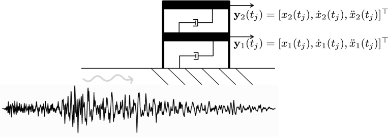
Figure 2: Shear building model. Horizontal displacements, velocities, and accelerations at the two floors are recorded.

The dynamic response of the structure is described by the following equations:

$$m\ddot{x}_{1}(t)+c_{1}\dot{x}_{1}(t)+k(2x_{1}(t)-x_{2}(t))=-mb(t)$$ (18a)

$$m\ddot{x}_{2}(t)+c_{2}\dot{x}_{2}(t)+k(x_{2}(t)-x_{1}(t))=-mb(t)$$ (18b)

where: $m=625$ ton is the mass of each floor; $k$ is the inter-storey stiffness; $b(t)$ is the ground acceleration signal; $c_{1}$ and $c_{2}$ are coefficients set to have $1\%$ damping over the two eigenmodes of the building model.

Seismic signals have been taken from the STEAD database [43]. Each seismogram $b(t)$ features the same time duration $T=60$ s and a sampling time step $\Delta t=0.01$ s. The dynamic system is not autonomous due to the presence of this external forcing term. We assume to know the input thanks to the seismic monitoring networks present in many countries, such as in Italy [44, 37]. On the contrary, we have made the assumption that the storey stiffness is unknown. For instance, when considering reinforced concrete structures, it is challenging to predict how cracking affects the moment of the inertia of column sections, or whether the modelling choices for boundaries have been adequate. Similarly, it is hard to guess how long term degradation effects may have altered the building properties over time. For this reason, we treat the value of the inter-storey stiffness as a stochastic variable featuring a uniform probability density function between $0.5\cdot 10^{6}$ kN$/$m and $2\cdot 10^{6}$ kN$/$m. Hence, the stiffness $k$ is the parameter to be here estimated together with the state vector $\mathbf{x}=[x_{1},x_{2},\dot{x}_{1},\dot{x}_{2}]^{\top}$. The second order Eqs. (18) can be rewritten at first order using these coordinates, and the dynamics of the system is accordingly described by $n=4$ variables corresponding to the lateral storey displacements and velocities.

To perform the joint estimation of this system, we have constructed a SINDy model for the function $\mathbf{f}$ describing at first order the system, as detailed in Algorithm 1, obtaining $\mathbf{f}\approx\boldsymbol{\Xi}^{\top}_{f}\boldsymbol{\Theta}^{\top}_{f}([\boldsymbol{\varkappa},b]^{\top})$, with $\boldsymbol{\varkappa}=[\mathbf{x},k]^{\top}$. Specifically, the snapshot matrix $\mathbf{X}_{\varkappa b}$ has been constructed by collecting in time the values of the augmented state vector $[\mathbf{x},k]^{\top}$ and for $I=20$ different values of $k$. Polynomial terms up to the second order have been employed in the definition of the function library $\boldsymbol{\Theta}_{f}$, as it can be demonstrated that they can describe the system dynamics, see, e.g. [25]. Hence, we have obtained a model for the observation operator $\mathbf{h}$ as in the following

$$\mathbf{y}=\begin{bmatrix}\mathbf{y}^{x}\\ \mathbf{y}^{\dot{x}}\\ \mathbf{y}^{\ddot{x}}\end{bmatrix}=\begin{bmatrix}\mathbf{B}_{x}\mathbf{x}\\ \mathbf{B}_{\dot{x}}\dot{\mathbf{x}}\\ \mathbf{B}_{\ddot{x}}(\boldsymbol{\Xi}^{\top}_{f}\boldsymbol{\Theta}^{\top}_{f}([\boldsymbol{\varkappa}^{\top},b]^{\top}))\end{bmatrix},$$ (19)

where: $\mathbf{B}_{x}$ and $\mathbf{B}_{\dot{x}}$ are the Boolean matrices that relate displacements and velocities to the observations of the system; $\mathbf{B}_{\ddot{x}}$ is the Boolean matrix that relates the accelerations computed by SINDy to the observed accelerations. The computation of the Jacobian matrices $\mathbf{F}$ and $\mathbf{H}$ has been done as described in Eqs. (15a) and 15b taking advantage of the use of polynomial functions in the library $\boldsymbol{\Theta}_{f}$.

The least square regression used to determine the SINDy weighting coefficients, see Eq. (13), is managed through the python open source package PySINDy [45]. The sparsity promoting regularisation term is set to $L=10^{-2}$. As expected, the adopted second-order library is perfectly suitable to model the dynamics of the system, accounting also for the dependence on $k$.

Hence, we have taken advantage of the combination of SINDy with EKF to perform the joint estimation of shear building whose stiffness is unknown. Specifically, we have taken as initial guess $k=1.01$ kN$/$m, overestimating by $20\%$ the target value. As previously mentioned, displacements, velocities and accelerations of both floors have been recorded. Although an identifiability assessment has not been carried out, see e.g. [46], the full observation of the system guarantees the possibility to estimate $k$. In future works, the intention is to explicitly perform an identifiability assessment, for example through the software DAISY [47].

To simulate the outcome of a real monitoring system, signals have been corrupted with white noise featuring a signal to noise ratio equal to $15$. Such level and type of noise is compatible with the use of, e.g., MEMS sensors [48]. Before running the online stage of Algorithm 2, we have initialised the state covariance matrix $\mathbf{P}(0)$, the process noise covariance matrix $\mathbf{Q}$, and the observation noise covariance matrix $\mathbf{R}$ as diagonal matrices. The values of the diagonal entries of these matrices are specified in the Appendix. The tuning of these quantities has been carried out through a trial-and-error procedure; however, automatic tuning procedures based for example on genetic algorithms [49] or on swarm intelligence [50], can be utilised.

The outcome of the estimation procedure is summarised in Fig. 3 for a seismogram randomly picked from the STEAD database. The mean value of the estimated parameter $\hat{k}$ converges to the target $\bar{k}$ in roughly 10 s reducing in the meanwhile the uncertainty of the estimation, measured by the variance $\sigma_{k}$. The system dynamics is precisely tracked as well, as illustrated in Fig. 4 in terms of a close-up of the kinematic quantities. A confidence interval for the acceleration estimates is not provided, because accelerations are not included in the state vector $\mathbf{x}$. Looking at the displacement and velocity of the first storey, it can be noted that the procedure is strongly tolerant to noise, being the filter estimates $\hat{x}_{1}$ and $\hat{\dot{x}}_{1}$ much closer to the noise-free version of the signals $\hat{\bar{y}}^{x}_{1}$ and $\hat{\bar{y}}^{\dot{x}}_{1}$ than the noise corrupted versions $\bar{y}^{x}_{1}$ and $\bar{y}^{\dot{x}}_{1}$, despite that in the first part of the analysis $k$ is not correctly calibrated yet. Clearly, the matching improved even more after the first $10$ s. The greater discrepancy between acquired recordings and EKF estimates of the accelerations has been due the impossibility of correcting the predicted accelerations, as lateral accelerations are not included in the state vector $\mathbf{x}$.

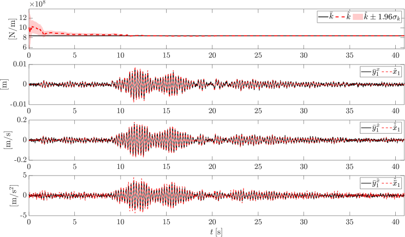
Figure 3: Shear building. In the top left corner, the shear building model is depicted, with the inter-storey stiffness to be calibrated highlighted in red. In the top right corner, the estimated parameter $\hat{k}_{1}$ is plotted in red against the target $\bar{k}_{1}$ in black. The red shaded area represents $95\%$ confidence interval of the estimates, determined using the posterior covariance. In the other graphs, the evolution of the system response tracked by the filter is plotted in red against the real system dynamics in black. For the sake of presentation, the outcomes of the $60$ s analyses are truncated after $40$ s.

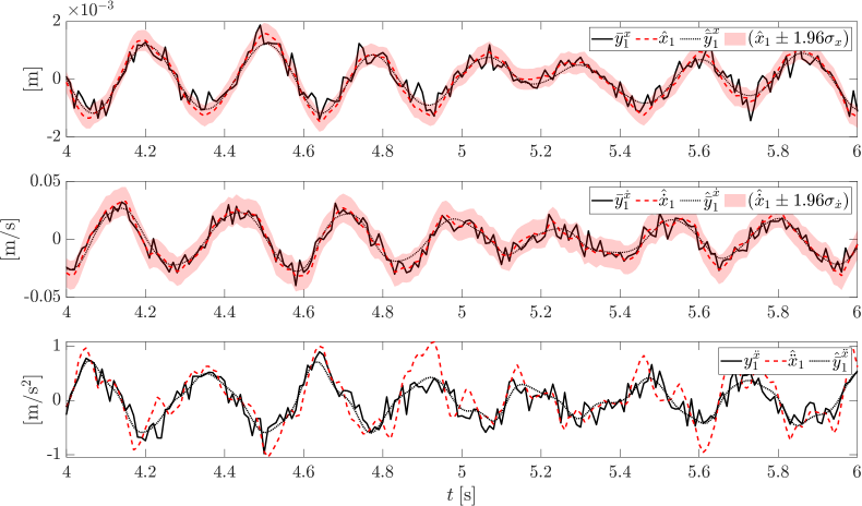
Figure 4: Shear building. Zoom in of Fig. 3: comparison between the evolution in time of the system response tracked by the filter (red dotted lines) and target one (black lines). Red shaded areas represent the $95\%$ confidence intervals determined using the posterior covariance. Black solid lines represent the noise corrupted signals, while black dotted lines their uncorrupted version.

Beyond the excellent estimation capabilities, the most intriguing aspects of the proposed procedure are its ease of use and the short execution time. Specifically, the Jacobian matrices have been straightforwardly determined (the reader may refer to [25] to understand the level of effort required to compute the Jacobian matrices for a simple system like this). Regarding the computational aspects, the execution of the procedure is approximately $40$ times faster than the physical process (lasting $60$ s when run on a workstation equipped with an Intel (R) Core${}^{\text{TM}}$, i7-2600 CPU @ 3.4 GHz with 16 GB RAM), moving towards real time monitoring in civil and mechanical engineering applications.

3.2 Partially observed nonlinear dynamic system

A second test case deals with a partially observed nonlinear dynamic system. The system comprises two coupled oscillators characterised by linear stiffness coefficient $k_{i}$, and linear damping coefficient $c_{i}$, with $i=1,2$. These oscillators are linked via linear and quadratic coupling terms controlled by the coefficients $\alpha$ and $\beta$, respectively. The coefficient $\gamma$ dictates instead the contribution of a cubic nonlinearity to the motion of one oscillator. The equations governing the free vibrations of the system are:

$$m_{1}\ddot{z}_{1}(t)+c_{1}\dot{z}_{1}(t)+k_{1}z_{1}(t)+\alpha z_{2}(t)=0,$$ (20a)

$$m_{2}\ddot{z}_{2}(t)+c_{2}\dot{z}_{2}(t)+k_{2}z_{2}(t)+\gamma z^{3}_{2}(t)+\alpha z_{1}(t)+\beta z^{2}_{1}(t)=0,$$ (20b)

for $t=(0,T]$, where: $m_{1}=1$; $m_{2}=1$; $k_{1}=1.0$; $c_{1}=10^{-2}$; $c_{2}=5\cdot 10^{-3}$; $\alpha=-10^{-1}$; $\beta=2\cdot 10^{-3}$; $\gamma=10^{-3}$; $T=200.0$. The time axis is discretised with a sampling time $\Delta T=10^{-2}$. Both the parameters and the time axis have been made dimensionless. Similarly to what considered in Sec. 3.1, the second order Eqs. (20) have been rewritten at first order with a simple change of coordinate, ı.e. $(\tilde{z}_{1},\tilde{z}_{2},\tilde{z}_{3},\tilde{z}_{4})=(z_{1},\dot{z}_{1},z_{2},\dot{z}_{2})$, so that the dynamics of the system is described by $n=4$ variables corresponding to the displacements and velocities of the two oscillators. It is worth stressing that, although addressing a real system is beyond the scope of this investigation, several microstructures feature nonlinear interactions between two modes, called internal resonances, that can be effectively modelled as in Eq.(20), see e.g. the case of MEMS gyroscope analysed in [51].

We have assumed to be able to observe only $y(t)=z_{1}(t)$. The aim is therefore to reconstruct the entire system dynamics $\mathbf{f}$ through SINDy by using only snapshots of $z_{1}$, thus considering realistic setting in which both $\mathbf{f}$ and $\mathbf{h}$ must be identified starting only from system observations, with the dimension of the observations smaller than the state of the system, ı.e. $o<n$. We make use of this example to show how to determine a SINDy model when the full state of the system can not be observed, and how to use this model to identify the system parameters. Such parameters can be related to unobserved system components, like the linear stiffness $k_{2}$ of the hidden oscillator and the coupling parameters $\alpha$ and $\beta$. Here, we have employed the time delay embedding technique to enrich the partial observation vector and recover the original dimensionality of the system state. After having trained a SINDy model on the new set of embedded-coordinates, we have proceeded with the system identification with EKF-SINDy.

3.2.1 Time-delay embedding

In general, (fully) learning $\mathbf{f}$ directly in its original dimension from lower dimensional measurements $\mathbf{y}$ is not possible. To tackle this issue, time-delay embedding techniques [10] can be adopted to lift the low-dimensional time series into a high-dimensional space where it is possible to recover hidden state components that might be fundamental to describe the dynamics [11]. In our context, we hope to recover features carrying on information about the unobserved oscillator.

Firstly, the time-delay embedding method is applied and the associated Hankel matrix is constructed by stacking time-shifted copies of the observed time series. Secondly, a Singular Value Decomposition (SVD) of this matrix is performed to extract time-delay coordinates approximating the Koopman operator in finite dimension [52], thereby providing a linearised description of the system dominant dynamics [26]. Indeed, the reference system formed by these time-delay coordinates is diffeomorphic to the original attractor of the system dynamics, under the conditions given by the Takens’ embedding theorem [53]. Lastly, this new set of coordinates can be leveraged by SINDy both in the training and prediction phases, to better capture the dynamics and to improve prediction performance [11].

Putting the method into practice, we report the outcome of the time-delay embedding including in the Hankel matrix the dependence on the stiffness $k_{2}$ of the unobserved oscillator, thus setting $\phi=k_{2}$. These embedded coordinates will be exploited to construct the SINDy model. For the $\iota$-th sample $\phi_{\iota}$, with $\iota=1,\ldots,I$, Eqs. (20) are numerically integrated in time for $T\leq T$. It is worth noting that, unlike what has been done here, the procedure does not strictly require to collect snapshots over the whole time axis. By collecting $z_{1}(\phi_{\iota},t_{j})$, for $j=1,\ldots,T$, we assemble the matrix:

$$\mathbf{A}_{\iota}=\begin{bmatrix}z_{1}(\phi_{\iota},t_{1})&z_{1}(\phi_{\iota},t_{2})&\cdots&z_{1}(\phi_{\iota},t_{T-w})\\ z_{1}(\phi_{\iota},t_{2})&z_{1}(\phi_{\iota},t_{3})&\cdots&z_{1}(\phi_{\iota},t_{T-w+1})\\ \vdots&\vdots&\ddots&\vdots\\ z_{1}(\phi_{\iota},t_{w})&z_{1}(\phi_{\iota},t_{w+1})&\cdots&z_{1}(\phi_{\iota},t_{T})\end{bmatrix}.$$ (21)

Thus, we construct the Hankel matrix $\mathbf{A}$ by stacking $\mathbf{A}=[\mathbf{A}_{1},\ldots,\mathbf{A}_{I}]\in\mathbb{R}^{w\times(T-w)I}$, and next we take its SVD:

$$\mathbf{A}=\mathbf{U}\mathbf{S}\mathbf{V}^{\top},$$ (22)

where: $\mathbf{U}\in\mathbb{R}^{w\times w}$ and $\mathbf{V}\in\mathbb{R}^{(T-w)I\times(T-w)}I$ are two orthogonal matrices whose columns are termed left and right singular vectors, respectively; ${\mathbf{S}}\in\mathbb{R}^{w\times(T-w)}I$ is a pseudo-diagonal matrix collecting the associated singular values.

For this case, we have considered $I=16$, $w=200$ and $\zeta=1$, where $w$ and $\zeta$ indicate the number of delay embeddings and the embedding period (ı.e, the number of lags in each successive embedding), respectively. The $I$ values of the parameter $k_{2}$ have been sampled in the range $[1.0,2.0]$ using a stratified sampling [54].

Performing the SVD on the Hankel matrix indicates that only $4$ dominant modes are responsible for the $99.97\%$ of the variance of $\mathbf{A}$, as illustrated by Fig. 5. This outcome aligns with the problem original dimension.In Fig. 5, we have also highlighted that the left singular values (reported in the boxes close to the corresponding singular values) resemble Legendre polynomials, as expected by choosing a small embedding period ($\zeta=1$) [55, 56].

Coming back to the time delay parameters $w$ and $d$, we can argue that our choices guaranteed to unfold the attractor in the embedding space [57] by satisfying the Taken’s embedding theorem condition on the number of delay embeddings $w>2n$. Indeed, this condition guarantees the existence of the diffeomorphism to the original system. A comparison of time-delayed coordinates with respect to the original (unobserved) ones is reported in Fig. 5. The similarity between these coordinates highlights that the time-delay coordinates adopted effectively allow for unfolding the attractor.

According to the singular value decay, we have truncated the SVD matrices to account just for the $n=4$ dominant modes. The selected singular values and the left singular vectors are collected in the matrices $\tilde{\mathbf{S}}\in\mathbb{R}^{n\times n}$ and $\tilde{\mathbf{U}}\in\mathbb{R}^{w\times n}$, respectively.

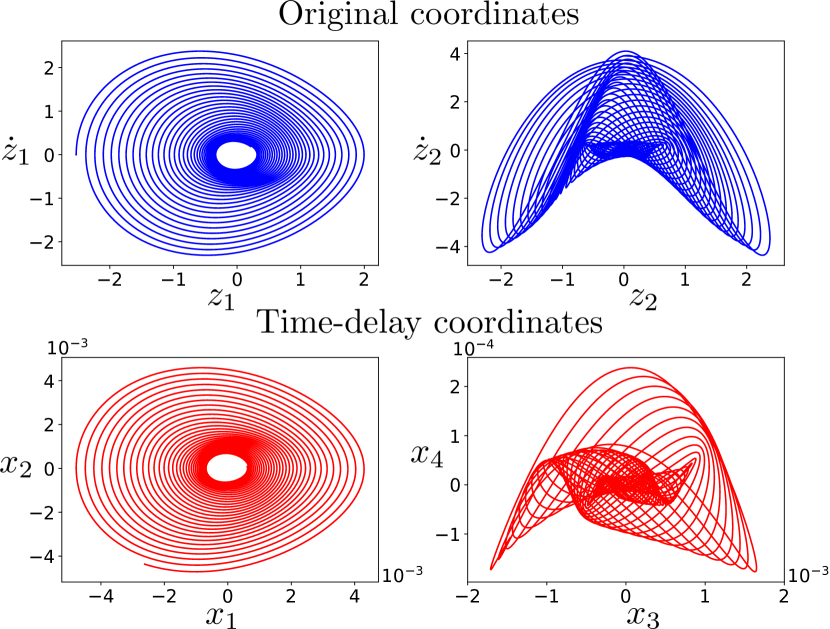
Figure 5: Nonlinear resonator. Dominant singular values and left singular vectors (left) and corresponding time-delay coordinates (right), obtained by performing the SVD on the Hankel matrix constructed by integrating the considered nonlinear dynamic system for $I=16$ values of $k_{2}$ sampled from $[1.0,2.0]$.

3.2.2 EKF-SINDy leveraging embedded coordinates

A SINDy model has then been trained by leveraging on the time-delayed coordinates to evolve the system dynamics. Specifically, the training has been performed after projecting the time series used to construct the Hankel matrix into the space spanned by the columns of $\tilde{\mathbf{U}}$ as in the following:

$$\mathbf{x}(t_{j})=\tilde{\mathbf{S}}^{-1}\tilde{\mathbf{U}}^{\top}\left(\mathbf{A}\mathbf{e}_{j}\right),$$ (23)

where $\mathbf{e}_{j}\in\mathbb{R}^{(T-w)I}$ is the basis vector extracting the $j$-th column of $\mathbf{A}$.

The state vector is then augmented with the corresponding parameter as $\boldsymbol{\varkappa}=\left[\mathbf{x}^{\top},\phi\right]^{\top}$. State data are collected in the matrix $\mathbf{X}_{\varkappa}\in~{}\mathbb{R}^{TI\times(n+1)}$ that is necessary for training the SINDy model. According to Algorithm 1, we use SINDy to build the function $\mathbf{f}\approx\boldsymbol{\Xi}_{f}\boldsymbol{\Theta}_{f}(\boldsymbol{\varkappa})$, describing the dynamics of the delayed coordinates. Polynomial terms up to the third order are included in $\boldsymbol{\Theta}_{f}$, due to the cubic nonlinearities present in the system (20). The sparsity promoting term has been set to $L=10^{-3}$. Interestingly, diminishing this regularisation term to $L=5\cdot 10^{-4}$ including more terms in the description of the dynamics, slightly improves the reconstruction capacity of SINDy but greatly deteriorates the identification capacity of the procedure. This suggests that the extra term included in the description of the system dynamics obtained for $L=5\cdot 10^{-4}$ does not have a physical meaning, but simply helps in fitting the collected time histories [26].

On the other hand, the function $\mathbf{h}$ extracting observations $z_{1}(t_{j})$ from the state variables $\mathbf{x}(t_{j})$ is known. Specifically, $\mathbf{h}$ is linear and it can be determined by inverting Eq. (23) as in the following

$$z_{1}(t_{j})=\mathbf{e}^{\top}_{1}\tilde{\mathbf{U}}\tilde{\mathbf{S}}\mathbf{x}(t_{j}),$$ (24)

where $\mathbf{e}_{1}\in\mathbb{R}^{w}$ is the basis vector extracting the first row of $\tilde{\mathbf{U}}$ or, in other words, the first component of each left singular vector in the vector space $\mathbb{R}^{w}$.

Finally, to apply the EKF-SINDy based joint estimation procedure, it is necessary to compute the Jacobian matrices $\mathbf{F}$ and $\mathbf{H}$. While $\mathbf{F}$ is computed as in Eq. (15a), $\mathbf{H}$ can be immediately derived by Eq. (24).

3.2.3 Estimation of the stiffness $k_{2}$ of the hidden oscillator

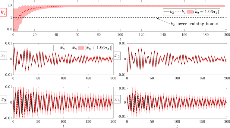
Figure 6: Nonlinear dynamic system, estimation of the resonator stiffness $\bar{k}=1.2$. In the top left corner, the nonlinear resonator model is depicted, with the resonator stiffness to be calibrated highlighted in red. In the top right corner, the estimated parameter $\hat{k}_{2}$ is plotted in red against the target $\bar{k}_{2}$ in black. The red shaded area represents the $95\%$ confidence interval of the estimates, determined using the posterior covariance. In the other graphs, the evolution of the (hidden) system respoonse tracked by the filter is plotted in red against the real system dynamics in black.

We have applied the EKF-SINDy procedure to estimate the stiffness $k_{2}$ of the hidden oscillator. In the offline phase, we have performed time-delay embedding and approximate the dynamic model $\mathbf{f}$ by training SINDy on the time-delayed coordinates. The parameters defining the operated time delay-embedded have been reported in Sec. 3.2.1. As previously specified, $k_{2}$ has been sampled from $[1.0,2.0]$.

We test our method for two instances $\bar{k}_{2}\in\{1.2,2.3\}$, whose results are reported in Fig. 6 and Fig. 8, respectively. The tuning parameters of the filter are reported in the Appendix.

For the test case $\bar{k}_{2}=1.2$, starting from an initial parameter guess outside the training range of SINDy and underestimating $\bar{k}_{2}$ by $25\%$, the EKF-SINDy method progressively increases accuracy and decreases uncertainty until $t=~{}50$, when it converges to the correct value. Similarly, it provides an accurate state estimate with uncertainty bounds that include the (partially observed) state of the system. We recall that data assimilation is limited to the observation of the displacement of the first oscillator, while the other quantities required to describe the system ($z_{2}$, $\dot{z}_{1}$ and $\dot{z}_{2}$) are unobserved. The target $\bar{\mathbf{x}}=[\bar{x}_{1},\bar{x}_{2},\bar{x}_{3},\bar{x}_{4}]^{\top}$ is reconstructed from the real dynamics of the system for sake of comparison with the filter estimates $\hat{\mathbf{x}}_{n}$. After convergence at $t=~{}50$, the predicted mean value of the state closely matches the evolution of the state and demonstrates robustness over the entire time horizon. The reconstructed $\hat{z}_{1}$ is plotted against the acquired measurements $\bar{z}_{1}$ in Fig. 7. demonstrating the noise tolerance of the procedure, with the filter estimate $\hat{z}_{1}$ closely aligning with the noise-free version of the signal $\hat{\bar{z}}_{1}$.

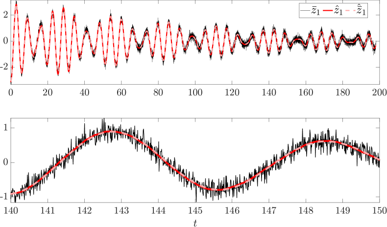
Figure 7: Nonlinear dynamic system, estimation of the resonator stiffness $\bar{k}=1.2$. Comparison between the observed variable $\bar{z}_{1}$ in black and its filter reconstruction $\hat{z}_{1}$ in red. The noise free version $\hat{\bar{z}}_{1}$ of the acquired measurements is depicted with a dotted line in pink.

Starting the identification process from an initial guess for $k_{2}$ outside the limits for which data have been collected in the offline phase, as shown in Algorithm 1, assesses the robustness of procedure. Operating outside such a training range is hardly achievable by other ML techniques like NNs [58, 59], which constitutes a major advantage of the proposed procedure. This advantage stems from the capacity of the retained SINDy library terms to describe the dominant dynamical behaviour of the system. Thus, these terms approximate the physical process that underlies the observed dynamics [5].

To further evaluate the capability of the proposed approach to function beyond the training range of SINDy, a second test case with $\bar{k}_{2}=2.3$ has been conducted. In this case, the initial guess for the stiffness of the second oscillator overestimated the correct value by $20\%$. Unlike the scenario with $\bar{f}_{2}=1.2$, the entire identification procedure was expected to operate outside the training range $[1.0,2.0]$ of SINDy. However, EKF-SINDy successfully performed the estimation of the system properties as illustrated in Fig. 8. In contrast, the estimation of the hidden state components $x_{3}$ and $x_{4}$ shows some degradation.

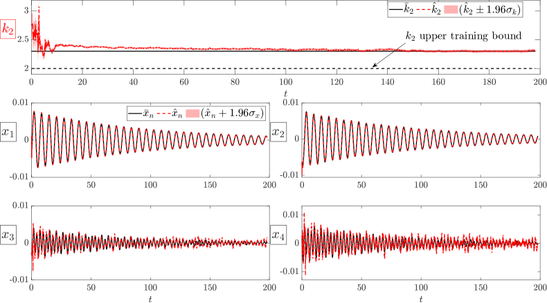
Figure 8: Nonlinear dynamic system, estimation of the resonator stiffness $\bar{k}=2.3$. See caption of Fig. 6 for further details.

3.2.4 Estimation of the parameters $\alpha$ and $\beta$ related to linear and quadratic coupling terms

To demonstrate the procedure capability of identifying more than one system parameter, we have simultaneously addressed the estimation of the linear and quadratic coupling terms $\alpha$ and $\beta$, while setting $k_{2}=1.95f_{1}$. In future work, we will investigating the internal resonances potentially arising for this frequency ratio as done in [51].

We have sampled $I=20$ values of $\alpha$ and $\beta$ to construct the Hankel matrix and to train SINDy on the time-delayed coordinates. Specifically, we have applied the Latin hypercube sampling across the domain $[0.005,0.5]^{2}$ with logarithmic scaling [54]. The logarithmic scaling has been used to put attention to cases featuring, possibly simultaneously, low values of $\alpha$ and $\beta$. Indeed, considering only high values of $\alpha$ and $\beta$ will possibly make the system response dynamics ruled by few dominant dynamic effects, precluding the investigation of potential interaction phenomena. As in previous cases, we have fixed the number $w$ of delay embeddings to $200$, and the embedding period $\zeta$ at $1$. The tuning of the filter is reported in the Appendix.

The outcome of the system identification, illustrated in Fig. 9, highlights the capacity of the EKF-SINDy procedure to simultaneously estimate $\alpha$ and $\beta$. The convergence in the estimation of $\alpha$ and $\beta$ occurs roughly at $t=50$. Before that point, the prediction of the hidden dynamic state components $x_{3}$ and $x_{4}$ is imprecise, as shown in Fig. 10. In contrast, there is no discrepancy observed between predicted and target values for the other hidden coordinates $x_{1}$ and $x_{2}$. These observations lead to conclude that enlarging the coordinates system from the number of observed variable, namely $1$, to the number of variables, namely $4$, is crucial to for correctly describing the dynamics of the system.

Figure 9: Nonlinear dynamic system, estimation of the parameters $\alpha$ and $\beta$ of the linear and quadratic coupling terms. In the top left corner, the nonlinear resonator model is depicted with highlighted the coupling parameters to be calibrated. In the top right corner, the estimated parameter $\hat{\alpha}$ is plotted in red against the target $\bar{\alpha}$ in black. Below, the estimated $\hat{\beta}$ is plotted in blue against the target $\bar{\beta}$ in black. The red and blue shaded area represents $95\%$ confidence interval of the estimates, determined using the posterior covariance. In the bottom right corner, a comparison between the observed variable $\bar{z}_{1}$ in black and its filter reconstruction $\hat{z}_{1}$ in red is reported. The noise free version $\hat{\bar{z}}_{1}$ of the acquired measurements is depicted with a dotted line in pink. A zoom in of this plot is reported on the left.

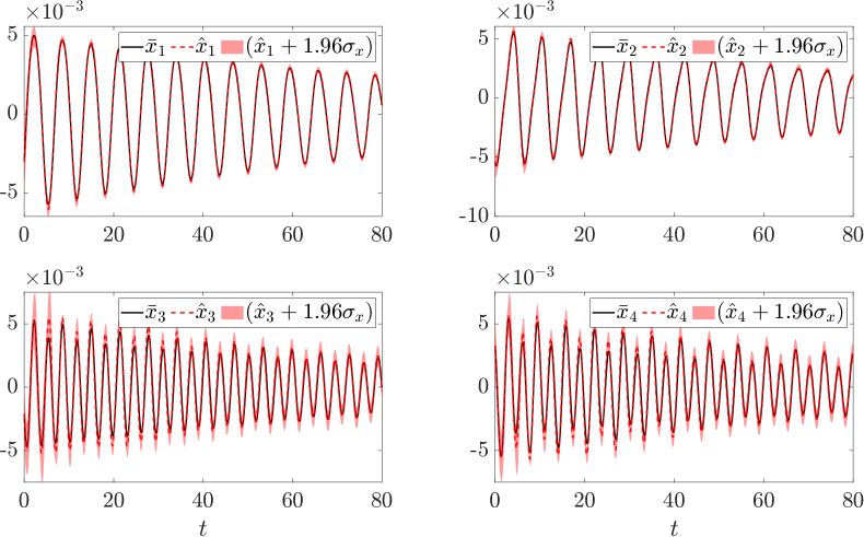
Figure 10: Nonlinear dynamic system, estimation of the parameters $\alpha$ and $\beta$ of the linear and quadratic coupling terms. The evolution of (hidden) system dynamics tracked by the filter is plotted in red against the real dynamics in black. The red shaded area represents $95\%$ confidence interval of the estimates determined using posterior covariance. For the sake of presentation, the outcomes are truncated at $t=80$.

4 Conclusions

In this work, we have proposed to empower the extended Kalman filter with the sparse identification of nonlinear dynamics (SINDy) to provide a robust, easy-to-use, and computationally inexpensive tool to enable the construction and update of digital twins. The procedure has been able to identify the dynamics of the system and their mechanical properties, providing confidence bounds for these quantities, by assimilating noisy and possibly partial observations.

We have demonstrated this capacity by addressing two case studies. First, we addressed a linear non-autonomous system consisting of a shear building model, frequently used in vibration monitoring of civil structures, excited by real seismograms. Last, we faced a partially observed nonlinear system identifying in a first analysis the stiffness of the unobserved resonator, and in a second analysis the linear and quadratic coupling coefficients of the two resonators. Interestingly, we have showed how the procedure yields good outcomes also when the identification was operated outside the training range of SINDy. This demonstrates robustness and superior generalization capabilities of the proposed method with respect to alternative machine learning strategies, which rely on fully black-box, data-driven approaches, as, e.g., neural networks. We have also shown how the time delay embedding can be used to to uplift the dimensionality of the partial observations thus enabling the full description of the system dynamics.

Future and challenging directions involve applying the method to experimental data, which requires extending the approach to handle high-dimensional data. Given that SINDy is sensitive to data dimensionality, the strategy is to integrate the method with suitable dimensionality reduction techniques, such as, e.g., proper orthogonal decomposition and/or autoencoders [13, 11]. This integration aims to employ SINDy within a reduced space while preserving the parametric dependency as in [14]. To further enhance the use of the procedure, we will also consider to employ automatic tuning procedures based on genetic algorithms [49] or on swarm intelligence [50] to perform the automatic tuning of the filter.

Code and data accessibility

The source code of the proposed method is made available from the GitHub repository:
https://github.com/ContiPaolo/EKF-SINDy [27].

APPENDIX A

We now report further information about the tuning of the EKF for the considered cases of study. In all cases, we have initialised the state covariance matrix $\mathbf{P}(0)$, the process noise covariance matrix $\mathbf{Q}$, and the observation noise covariance matrix $\mathbf{R}$ as diagonal matrices. In Tabs. A.1-A.3, the diagonal terms of these matrices are gathered.

Shear building
$x_{1},x_{2},\dot{x}_{1},\dot{x}_{2}$	$10^{-8}$
$k_{1}$	$10^{-2}$
Nonlinear dynamic
system
$\bar{k}_{2}=1.2$
$x_{1},x_{2},x_{3},x_{4}$	$10^{-6}$
$k_{2}$	$10^{-2}$
$\bar{k}_{2}=2.3$
$x_{1}$	$10^{-6}$
$x_{2}$	$10^{-6}$
$x_{3}$	$10^{-6}$
$x_{4}$	$10^{-6}$
$k_{2}$	$2\cdot 10^{-6}$
$\alpha$, $\beta$
$x_{1}$	$10^{-10}$
$x_{2}$	$10^{-10}$
$x_{3}$	$10^{-10}$
$x_{4}$	$10^{-10}$
$\alpha$	$10^{-1}$
$\beta$	$10^{-1}$

Table A. 1: Initial covariance $\mathbf{P}(0)$, diagonal terms. In the left column, we specify the augmented state quantities to which these values are related.

       Shear building $x_{1},x_{2},\dot{x}_{1},\dot{x}_{2}$ $5\cdot 10^{-3}$ $k_{1}$ $10^{-8}$ Nonlinear dynamic system $\bar{k}_{2}=1.2$ $x_{1},x_{2},x_{3},x_{4}$ $10^{-7}$ $k_{2}$ $10^{-7}$ $\bar{k}_{2}=2.3$ $x_{1}$ $10^{-10}$ $x_{2}$ $10^{-10}$ $x_{3}$ $10^{-8}$ $x_{4}$ $10^{-8}$ $k_{2}$ $2\cdot 10^{-6}$ $\alpha$, $\beta$ $x_{1}$ $5\cdot 10^{-10}$ $x_{2}$ $5\cdot 10^{-10}$ $x_{3}$ $2\cdot 10^{-8}$ $x_{4}$ $3\cdot 10^{-8}$ $\alpha$ $3\cdot 10^{-1}$ $\beta$ $3\cdot 10^{-1}$ Table A. 2: Process noise $\mathbf{Q}$, diagonal terms. In the left column, we specify the augmented state quantities to which these values are related.        Shear building $x_{1}$ $10^{-3}$ $x_{2}$ $10^{-3}$ $\dot{x}_{1}$ $10^{-3}$ $\dot{x}_{2}$ $10^{-3}$ $\ddot{x}_{1}$ $10^{3}$ $\ddot{x}_{2}$ $10^{3}$ Nonlinear dynamic system $\bar{k}_{2}=1.2$ $z_{1}$ $10^{-7}$ $\bar{k}_{2}=2.3$ $z_{1}$ $5\cdot 10^{-4}$ $\alpha$, $\beta$ $z_{1}$ $3\cdot 10^{-1}$ Table A. 3: Measurement noise $\mathbf{R}$, diagonal terms. In the left column, we specify the observed quantities to which these values are related.

References

- [1] D. J. Wagg, K. Worden, R. J. Barthorpe, P. Gardner, Digital Twins: State-of-the-Art and Future Directions for Modeling and Simulation in Engineering Dynamics Applications, ASCE-ASME Journal of Risk and Uncertainty in Engineering Systems, Part B: Mechanical Engineering 6 (3) (2020) 030901. doi:10.1115/1.4046739.
- [2] M. Torzoni, M. Tezzele, S. Mariani, A. Manzoni, K. E. Willcox, A digital twin framework for civil engineering structures, Computer Methods in Applied Mechanics and Engineering 418 (2024) 116584. doi:10.1016/j.cma.2023.116584.
- [3] L. Guastoni, J. Rabault, P. Schlatter, H. Azizpour, R. Vinuesa, Deep reinforcement learning for turbulent drag reduction in channel flows, The European Physical Journal E 46 (2023) 27. doi:10.1140/epje/s10189-023-00285-8.
- [4] M. I. Jordan, T. M. Mitchell, Machine learning: Trends, perspectives, and prospects, Science 349 (6245) (2015) 255–260. doi:10.1126/science.aaa8415.
- [5] S. L. Brunton, J. L. Proctor, J. N. Kutz, Discovering governing equations from data by sparse identification of nonlinear dynamical systems, Proceedings of the National Academy of Sciences 113 (15) (2016) 3932–3937. doi:10.1073/pnas.1517384113.
- [6] A. Olivier, M. D. Shields, L. Graham-Brady, Bayesian neural networks for uncertainty quantification in data-driven materials modeling, Computer Methods in Applied Mechanics and Engineering 386 (2021) 114079. doi:10.1016/j.cma.2021.114079.
- [7] D. Wagg, C. Burr, J. Shepherd, Z. X. Conti, M. Enzer, S. Niederer, The philosophical foundations of digital twinning (2024). doi:https://doi.org/10.31224/3500.
- [8] R. E. Kalman, A new approach to linear filtering and prediction problems, Journal of Basic Engineering 82 (1) (1960) 35–45. doi:10.1115/1.3662552.
- [9] E. Wan, R. Van Der Merwe, The unscented Kalman filter for nonlinear estimation, in: Proceedings of the IEEE 2000 Adaptive Systems for Signal Processing, Communications, and Control Symposium (Cat. No.00EX373), 2000, pp. 153–158. doi:10.1109/ASSPCC.2000.882463.
- [10] S. L. Brunton, B. W. Brunton, J. L. Proctor, E. Kaiser, J. N. Kutz, Chaos as an intermittently forced linear system, Nature Communications 8 (1) (2017) 19. doi:10.1038/s41467-017-00030-8.
- [11] J. Bakarji, K. Champion, J. Nathan Kutz, S. L. Brunton, Discovering governing equations from partial measurements with deep delay autoencoders, Proceedings of the Royal Society A 479 (2276) (2023) 20230422.
- [12] J. P. Williams, O. Zahn, J. N. Kutz, Sensing with shallow recurrent decoder networks, arXiv preprint arXiv:2301.12011 (2023).
- [13] K. Champion, B. Lusch, J. N. Kutz, S. L. Brunton, Data-driven discovery of coordinates and governing equations, Proceedings of the National Academy of Sciences 116 (45) (2019) 22445–22451.
- [14] P. Conti, G. Gobat, S. Fresca, A. Manzoni, A. Frangi, Reduced order modeling of parametrized systems through autoencoders and SINDy approach: continuation of periodic solutions, Computer Methods in Applied Mechanics and Engineering 411 (2023) 116072. doi:https://doi.org/10.1016/j.cma.2023.116072.
- [15] H. Coskun, F. Achilles, R. DiPietro, N. Navab, F. Tombari, Long short-term memory Kalman filters: Recurrent neural estimators for pose regularization, in: 2017 IEEE International Conference on Computer Vision (ICCV), October 22-29, Venezia, Italy, 2017, pp. 5525–5533. doi:10.1109/ICCV.2017.589.
- [16] W. Liu, Z. Lai, K. Bacsa, E. Chatzi, Neural extended Kalman filters for learning and predicting dynamics of structural systems, Structural Health Monitoring 23 (2) (2024) 1037–1052. doi:10.1177/14759217231179912.
- [17] R. Krishnan, U. Shalit, D. Sontag, Structured inference networks for nonlinear state space models, in: Proceedings of the Thirty-First AAAI Conference on Artificial Intelligence, February 4-9, San Francisco, California USA, Vol. 31, 2017.
- [18] E. Kaiser, J. N. Kutz, S. L. Brunton, Sparse identification of nonlinear dynamics for model predictive control in the low-data limit, Proceedings of the Royal Society A: Mathematical, Physical and Engineering Sciences 474 (2219) (2018) 20180335. doi:10.1098/rspa.2018.0335.
- [19] J. Wang, J. Moreira, Y. Cao, B. Gopaluni, Time-variant digital twin modeling through the Kalman-generalized sparse identification of nonlinear dynamics, in: 2022 American Control Conference (ACC), June 8-10, Atlanta, Georgia, USA, 2022, pp. 5217–5222. doi:10.23919/ACC53348.2022.9867786.
- [20] A. Vizzaccaro, G. Gobat, A. Frangi, C. Touzé, Direct parametrisation of invariant manifolds for non-autonomous forced systems including superharmonic resonances, Nonlinear Dynamics 112 (2024) 6255–6290. doi:10.1007/s11071-024-09333-0.
- [21] L. Rosafalco, M. Torzoni, A. Manzoni, S. Mariani, A. Corigliano, Online structural health monitoring by model order reduction and deep learning algorithms, Computers & Structures 255 (2021) 106604. doi:10.1016/j.compstruc.2021.106604.
- [22] L. Rosafalco, A. Manzoni, S. Mariani, A. Corigliano, Combined Model Order Reduction Techniques and Artificial Neural Network for Data Assimilation and Damage Detection in Structures, Springer International Publishing, Cham, 2022, pp. 247–259. doi:10.1007/978-3-030-70787-3\_16.
- [23] F. Abdullah, P. D. Christofides, Real-time adaptive sparse-identification-based predictive control of nonlinear processes, Chemical Engineering Research and Design 196 (2023) 750–769. doi:10.1016/j.cherd.2023.07.011.
- [24] N. Schmidt, P. Hennig, J. Nick, F. Tronarp, The rank-reduced Kalman filter: Approximate dynamical-low-rank filtering in high dimensions, in: Advances in Neural Information Processing Systems 36 pre-proceedings (Neurips 2023), December 10-16, New Orleans, Louisiana, USA, 2023.
- [25] L. Rosafalco, S. E. Azam, S. Mariani, A. Corigliano, System identification via unscented Kalman filtering and model class selection, ASCE-ASME Journal of Risk and Uncertainty in Engineering Systems, Part A: Civil Engineering 10 (1) (2024) 04023063. doi:10.1061/AJRUA6.RUENG-1085.
- [26] K. P. Champion, S. L. Brunton, J. N. Kutz, Discovery of nonlinear multiscale systems: Sampling strategies and embeddings, SIAM Journal on Applied Dynamical Systems 18 (1) (2019) 312–333. doi:10.1137/18M1188227.
- [27] L. Rosafalco, P. Conti, EKF-SINDy, https://github.com/ContiPaolo/SINDy-EKF (2024).
- [28] D. Simon, Nonlinear Kalman filtering, John Wiley & Sons, Ltd, 2006, Ch. 5, pp. 121–148. doi:10.1002/0470045345.ch13.
- [29] A. Corigliano, R. Ardito, C. Comi, A. Frangi, A. Ghisi, S. Mariani, Accelerometers, John Wiley & Sons, Ltd, 2018, Ch. 4, pp. 91–108. doi:10.1002/9781119053828.ch4.
- [30] S. W. Doebling, C. Farrar, M. Prime, A summary review of vibration–based damage identification methods, The Shock and Vibration Digest 30 (1998) 91–105. doi:10.1177/058310249803000201.
- [31] D. Simon, The discrete–time Kalman filter, John Wiley & Sons, Ltd, 2006, Ch. 5, pp. 121–148. doi:10.1002/0470045345.ch5.
- [32] D. A. Messenger, D. M. Bortz, Weak SINDy for partial differential equations, Journal of Computational Physics 443 (2021) 110525. doi:10.1016/j.jcp.2021.110525.
- [33] U. Fasel, J. N. Kutz, B. W. Brunton, S. L. Brunton, Ensemble-SINDy: Robust sparse model discovery in the low-data, high-noise limit, with active learning and control, Proceedings of the Royal Society A: Mathematical, Physical and Engineering Sciences 478 (2260) (2022) 20210904. doi:10.1098/rspa.2021.0904.
- [34] S. M. Hirsh, D. A. Barajas-Solano, J. N. Kutz, Sparsifying priors for Bayesian uncertainty quantification in model discovery, Royal Society Open Science 9 (2) (2022) 211823. doi:10.1098/rsos.211823.
- [35] L. M. Gao, U. Fasel, S. L. Brunton, J. N. Kutz, Convergence of uncertainty estimates in ensemble and Bayesian sparse model discovery (2023). arXiv:2301.12649.
- [36] S. Mariani, A. Corigliano, Impact induced composite delamination: state and parameter identification via joint and dual extended Kalman filters, Computer Methods in Applied Mechanics and Engineering 194 (50) (2005) 5242–5272. doi:10.1016/j.cma.2005.01.007.
- [37] A. D’Alessandro, A. Costanzo, C. Ladina, F. Buongiorno, M. Cattaneo, S. Falcone, C. La Piana, S. Marzorati, S. Scudero, G. Vitale, S. Stramondo, C. Doglioni, Urban seismic networks, structural health and cultural heritage monitoring: The national earthquakes observatory (INGV, Italy) experience, Frontiers in Built Environment 5 (2019) 127. doi:10.3389/fbuil.2019.00127.
- [38] S. Eftekhar Azam, E. Chatzi, C. Papadimitriou, A dual Kalman filter approach for state estimation via output-only acceleration measurements, Mechanical Systems and Signal Processing 60-61 (2015) 866–886. doi:10.1016/j.ymssp.2015.02.001.
- [39] V. Dertimanis, E. Chatzi, S. Eftekhar Azam, C. Papadimitriou, Input-state-parameter estimation of structural systems from limited output information, Mechanical Systems and Signal Processing 126 (2019) 711–746. doi:10.1016/j.ymssp.2019.02.040.
- [40] J. Castiglione, R. Astroza, S. Eftekhar Azam, D. Linzell, Auto-regressive model based input and parameter estimation for nonlinear finite element models, Mechanical Systems and Signal Processing 143 (2020) 106779. doi:10.1016/j.ymssp.2020.106779.
- [41] M. Ebrahimzadeh Hassanabadi, Z. Liu, S. Eftekhar Azam, D. Dias-da Costa, A linear Bayesian filter for input and state estimation of structural systems, Computer-Aided Civil and Infrastructure Engineering 38 (13) (2023) 1749–1766. doi:10.1111/mice.12973.
- [42] European commitee for standardization, Eurocode 8: design of structures for earthquake resistance - part 1: general rules, seismic actions and rules for buildings (2003) 66–74.
- [43] S. M. Mousavi, Y. Sheng, W. Zhu, G. C. Beroza, STanford EArthquake Dataset (STEAD): A global data set of seismic signals for AI, IEEE Access 7 (2019) 179464–179476. doi:10.1109/ACCESS.2019.2947848.
- [44] P. Pierleoni, S. Marzorati, C. Ladina, S. Raggiunto, A. Belli, L. Palma, M. Cattaneo, S. Valenti, Performance evaluation of a low-cost sensing unit for seismic applications: Field testing during seismic events of 2016-2017 in central Italy, IEEE Sensors Journal 18 (16) (2018) 6644–6659. doi:10.1109/JSEN.2018.2850065.
- [45] A. Kaptanoglu, B. de Silva, U. Fasel, K. Kaheman, A. Goldschmidt, J. Callaham, C. Delahunt, Z. Nicolaou, K. Champion, J.-C. Loiseau, J. Kutz, S. Brunton, PySINDy: A comprehensive python package for robust sparse system identification, Journal of Open Source Software 7 (69) (2022) 3994. doi:10.21105/joss.03994.
- [46] M. N. Chatzis, E. N. Chatzi, A. W. Smyth, On the observability and identifiability of nonlinear structural and mechanical systems, Structural Control and Health Monitoring 22 (3) (2015) 574–593. doi:10.1002/stc.1690.
- [47] G. Bellu, M. P. Saccomani, S. Audoly, L. D’Angió, DAISY: A new software tool to test global identifiability of biological and physiological systems, Computer Methods and Programs in Biomedicine 88 (1) (2007) 52–61. doi:10.1016/j.cmpb.2007.07.002.
- [48] A. D’Alessandro, G. Vitale, S. Scudero, R. D’Anna, A. Costanza, A. Fagiolini, L. Greco, Characterization of MEMS accelerometer self-noise by means of PSD and Allan variance analysis, in: 2017 7th IEEE International Workshop on Advances in Sensors and Interfaces (IWASI), June 15-16, Vieste, Italy, 2017, pp. 159–164. doi:10.1109/IWASI.2017.7974238.
- [49] K. Rapp, P.-O. Nyman, Optimization of extended Kalman filter for improved thresholding performance, IFAC Proceedings Volumes 36 (18) (2003) 119–124, 2nd IFAC Conference on Control Systems Design (CSD ’03), Bratislava, Slovak Republic, 7-10 September 2003. doi:10.1016/S1474-6670(17)34655-4.
- [50] Y. Laamari, K. Chafaa, B. Athamena, Particle swarm optimisation of an extended Kalman filter for speed and rotor flux estimation of an induction motor drive, Electrical engineering 97 (2015) 129–139. doi:10.1007/s00202-014-0322-1.
- [51] G. Gobat, V. Zega, P. Fedeli, L. Guerinoni, C. Touzé, A. Frangi, Reduced order modelling and experimental validation of a MEMS gyroscope test-structure exhibiting 1:2 internal resonance, Scientific Reports 11 (2021) 16390. doi:10.1038/s41598-021-95793-y.
- [52] D. Dylewsky, E. Kaiser, S. L. Brunton, J. N. Kutz, Principal component trajectories for modeling spectrally continuous dynamics as forced linear systems, Phys. Rev. E 105 (2022) 015312. doi:10.1103/PhysRevE.105.015312.
- [53] F. Takens, Detecting strange attractors in turbulence, in: D. Rand, L.-S. Young (Eds.), Dynamical Systems and Turbulence, Warwick 1980, Springer Berlin Heidelberg, Berlin, Heidelberg, 1981, pp. 366–381.
- [54] A. Saltelli, M. Ratto, T. Andres, F. Campolongo, J. Cariboni, D. Gatelli, M. Saisana, S. Tarantola, Experimental designs, in: Global Sensitivity Analysis. The Primer, John Wiley & Sons, Ltd, 2007, Ch. 2, pp. 53–107. doi:10.1002/9780470725184.ch2.
- [55] R. Vautard, M. Ghil, Singular spectrum analysis in nonlinear dynamics, with applications to paleoclimatic time series, Physica D: Nonlinear Phenomena 35 (3) (1989) 395–424.
- [56] D. S. Broomhead, G. P. King, Extracting qualitative dynamics from experimental data, Physica D: Nonlinear Phenomena 20 (2-3) (1986) 217–236.
- [57] H.-g. Ma, C.-z. Han, Selection of embedding dimension and delay time in phase space reconstruction, Frontiers of Electrical and Electronic Engineering in China 1 (2006) 111–114.
- [58] L. Rosafalco, M. Torzoni, A. Manzoni, S. Mariani, A. Corigliano, A Self-adaptive Hybrid Model/data-Driven Approach to SHM Based on Model Order Reduction and Deep Learning, Springer International Publishing, Cham, 2022, pp. 165–184. doi:10.1007/978-3-030-81716-9\_8.
- [59] M. Torzoni, L. Rosafalco, A. Manzoni, S. Mariani, A. Corigliano, SHM under varying environmental conditions: an approach based on model order reduction and deep learning, Computers & Structures 266 (2022) 106790. doi:10.1016/j.compstruc.2022.106790.