Geometric Observability of Hypergraphs

Joshua Pickarda, Cooper Stansburya, Amit Suranab,
Indika Rajapakseac, and Anthony Blochc
aDepartment of Computational Medicine and Bioinformatics, University of Michigan, Ann Arbor MI, USA
bRTX Technology Research Center, East Hartford, CT USA
cDepartment of Mathematics, University of Michigan, Ann Arbor MI, USA

Abstract

In this paper we consider aspects of geometric observability for hypergraphs, extending our earlier work from the uniform to the nonuniform case. Hypergraphs, a generalization of graphs, allow hyperedges to connect multiple nodes and unambiguously represent multi-way relationships which are ubiquitous in many real-world networks including those that arise in biology. We consider polynomial dynamical systems with linear outputs defined according to hypergraph structure, and we propose methods to evaluate local, weak observability.

Key words: Obervability, networks, hypergraphs.

1 INTRODUCTION

We consider here geometric aspects of observability with applications to hypergraphs motivated by biological networks. In particular, we consider nonuniform hypergraphs in which hyperedges can contain arbitrary finite number of nodes. This extends our work in Pickard, Surana, et al. (2023) which was restricted to observability analysis of uniform hypergraphs.

Hypergraphs extend classical graph theory by allowing hyperedges to have more than two vertices. This is important because may complex systems cannot be described by pairwise interactions only. Examples include social networks as well as complex physical and biological networks such as polymers and proteins. In Chen et al. (2021) we consider a mouse neuron model as well as interaction in the human genome which can be captured by hypergraph models. Allowing hypergraphs to be nonuniform allows one to capture the dynamics of complex asymmetrical systems.

Two fundamental questions arise when considering nonuniform hypergraph observability:

  • (Q1) Is a set of sensor nodes sufficient to render a network observable?

  • (Q2) How do higher order interactions contribute to observability?

Observability of networks has been considered from an array of perspectives; see A. N. Montanari and Aguirre (2020) and references therein. To address Q1, structural observability utilizes network topology Lin (1974); dynamic observability applies classical matrix properties, particle filtering A. Montanari and Aguirre (2019), or the observability Gramian Summers and Lygeros (2014); and topological observability explores the relationship between observability and graph topologies, Liu et al. (2013); Su et al. (2017). Despite the array of approaches, hypergraph observability and Q2 remain relatively unexplored.

To investigate Q2, this paper makes the following contributions:

  • We propose a multitensor representation of the adjacency structure and dynamics of nonuniform hypergraphs.

  • We develop a nonlinear observability test for nonuniform hypergraphs and demonstrate it on several canonical hypergraph topologies.

We focus on the concept of weak local observability for polynomial systems, and to overcome the limitations of local observability, our computations leverage symbolic calculations to offer a global observability test.

We begin with necessary background on nonlinear observability (Section 2) and uniform hypergraphs (Section 3). We extend these results to non-uniform hypergraphs, where we develop our calculations for the observability of nonuniform hypergraphs (Section 4).

2 NONLINEAR OBSERVABILITY BACKGROUND

Nonlinear controllability and observability were introduced in the seminal work Hermann and Krener (1977); see the work of Baillieul (1981) for polynomial dynamics. In contrast to linear systems, nonlinear observability, which is based similarly on the distinguishability of system states, has multiple varieties, such as local, weak, and global observability, Hermann and Krener (1977); Sontag (1984); Gerbet and Röbenack (2020). Unfortunately, unlike the linear case where the Kalman rank condition or Popov-Belevitch-Hautus test simply determine observability, no easy criteria exist for nonlinear systems.

Consider the affine control system $\Sigma$,

$$\Sigma\begin{cases}\dot{\mathbf{x}}=\mathbf{f}(\mathbf{x},\mathbf{u})=\mathbf{h}_{0}(\mathbf{x})+\sum_{i=1}^{k}\mathbf{h}_{i}(\mathbf{x})u_{i}\\ \mathbf{y}=\mathbf{g}(\mathbf{x})\end{cases}$$

where, $\mathbf{u}=(u_{1},\dots,u_{k})^{\prime}\in\mathbb{R}^{k}$ denotes the input vector, $\mathbf{x}\in M\subset\mathbb{R}^{n}$ is the state vector and $\mathbf{y}\in\mathbb{R}^{m}$ is the output/measurement vector. We assume that $\Sigma$ is analytic, i.e., the functions $\mathbf{h}_{i}:M\rightarrow M,i=0,\dots,k$ and $g_{i}:M\rightarrow\mathbb{R},i=1,\dots,m$ where $\mathbf{g}=(g_{1},\dots,g_{m})^{\prime}$ are assumed to be analytic functions defined on $M$. We also have to assume $\Sigma$ is complete, that is, for every bounded measurable input $\mathbf{u}(t)$ and every $\mathbf{x}_{0}\in M$ there exists a solution $\mathbf{x}(t)$ of $\Sigma$ such that $\mathbf{x}(0)=\mathbf{x}_{0}$ and $\mathbf{x}(t)\in M$ for all $t\in\mathbb{R}$. We review different notions of observability from Anguelova (2004) which are equivalent to those introduced in Hermann and Krener (1977), but use a slightly different terminology.

Definition 1

Let $U$ be an open subset of $M$. A pair of points $\mathbf{x}_{0}$ and $\mathbf{x}_{1}$ in $M$ are called $U$-distinguishable if there exists a measurable input $\mathbf{u}(t)$ defined on the interval $[0,T]$ that generates solutions $\mathbf{x}_{0}(t)$ and $\mathbf{x}_{1}(t)$ of system $\Sigma$ satisfying $\mathbf{x}_{i}(0)=\mathbf{x}_{i},i=0,1$ such that $\mathbf{x}_{i}(t)\in U$ for $t\in[0,T]$ and $\mathbf{g}(\mathbf{x}_{0}(t))\neq\mathbf{g}(\mathbf{x}_{1}(t))$ for some $t\in[0,T]$. We denote by $I(\mathbf{x}_{0},U)$ all points $\mathbf{x}_{1}\in U$ that are not $U$–distinguishable from $\mathbf{x}_{0}$

Definition 2

The system $\Sigma$ is observable at $\mathbf{x}_{0}\in M$ if $I(\mathbf{x}_{0},M)=\mathbf{x}_{0}$.

Definition 3

The system $\Sigma$ is locally observable at $\mathbf{x}_{0}\in M$ if for every open neighbourhood $U$ of $\mathbf{x}_{0}$, $I(\mathbf{x}_{0},U)=\mathbf{x}_{0}$

Local observability implies observability. On the other hand, since $U$ can be chosen arbitrarily small, local observability implies that we can distinguish between neighboring points instantaneously. Both the definitions above ensure that a point $\mathbf{x}_{0}\in M$ can be distinguished from every other point in $M$. It is often sufficient to distinguish between neighbours in $M$, which leads to the following two notions of observability.

Definition 4

The system $\Sigma$ is weakly observable at $\mathbf{x}_{0}\in M$ if $\mathbf{x}_{0}$ has an open neighbourhood $U$ such that $I(\mathbf{x}_{0},M)\bigcap U=\mathbf{x}_{0}$.

Definition 5

The system $\Sigma$ is locally weakly observable at $\mathbf{x}_{0}\in M$ if $\mathbf{x}_{0}$ has an open neighbourhood $U$ such that for every open neighbourhood $V$ of $\mathbf{x}_{0}$ contained in $U$, $I(\mathbf{x}_{0},V)=\mathbf{x}_{0}$.

As we can set $U=M$, local observability implies local weak observability. The local weakly observability lends itself to a simple algebraic test. Let $\mathcal{H}$ be the observation space,

$\displaystyle\mathcal{H}$ $\displaystyle=$ $\displaystyle\{L_{\mathbf{h}_{i_{1}}}L_{\mathbf{h}_{i_{2}}}\cdots L_{\mathbf{h}_{i_{r}}}(g_{i}):r\geq 0,i_{j}=0,\cdots,k,$
$\displaystyle i=1,\cdots,m\}$

where $L_{f}$ denotes the Lie derivative w.r.t. vector field $f$, and let

$$d\mathcal{H}=\mbox{span}_{\mathbb{R}_{x}}\{d\phi:\phi\in\mathcal{H}\}$$

be the space spanned by the gradients of the elements of $\mathcal{H}$, where $\mathbb{R}_{x}$ is the space of meromorphic functions on $M$. The following result was proved in Hermann and Krener (1977), see Theorems $3.1$ and $3.11$.

Theorem 1

The analytic system $\Sigma$ is locally weakly observable for all $\mathbf{x}$ in an open dense set of $M$ if and only if $dim_{\mathbb{R}_{x}}(d\mathcal{H})=n$.

Remark 1

Here $\mbox{dim}_{\mathbb{R}_{x}}(d\mathcal{H})$ is the generic or maximal rank of $d\mathcal{H}$, that is, $\mbox{dim}_{\mathbb{R}_{x}}(d\mathcal{H})=\max_{\mathbf{x}\in M}(dim_{\mathbb{R}}d\mathcal{H}(\mathbf{x}))$.

For system $\Sigma$ with no control inputs, i.e. $\mathbf{h}_{i}\equiv 0,i=1,\cdots,k$ the condition for local weak observability simplifies to checking,

$$\mbox{rank}(\mathcal{O}(\mathbf{x}))=n,$$ (1)

where $\mathcal{O}(\mathbf{x})$ is the nonlinear observability matrix (NOM),

$$\mathcal{O}(\mathbf{x})=\nabla_{\mathbf{x}}\begin{pmatrix}L^{0}_{\mathbf{h}_{0}}\mathbf{g}(\mathbf{x})\\ L^{1}_{\mathbf{h}_{0}}\mathbf{g}(\mathbf{x})\\ \vdots\\ L^{r}_{\mathbf{h}_{0}}\mathbf{g}(\mathbf{x})\end{pmatrix},$$ (2)

for some $r\in\mathbb{Z}$. One can use symbolic computation to check the generic rank condition (1) as performed by Sedoglavic’s algorithm, Sedoglavic (2001).

Remark 2

In general the value of $r$ to use in (2) is not known apriori. For an analytic system $\Sigma$, $r$ can be set to the state dimension $n$, see Theorem $4.1$ in Anguelova (2004).

Remark 3

For a polynomial system $\Sigma$, observability has also been studied from the perspective of algebraic geometry, see Gerbet and Röbenack (2020) and references therein.

We adopt the use of local weak observability as the notion of nonlinear observability throughout the remainder of this paper.

3 UNIFORM HYPERGRAPHS

A undirected hypergraph is given by $\mathcal{G}=\{\mathcal{V},\mathcal{E}\}$ where $\mathcal{V}$ is a finite set and $\mathcal{E}\subseteq\mathcal{P}(\mathcal{V})\setminus\{\emptyset\}$, the power set of $\mathcal{V}$ (i.e. the set of all subsets of $\mathcal{V}$). The elements of $\mathcal{V}$ are called the nodes, and the elements of $\mathcal{E}$ are called the hyperedges. Cardinality $|e|$ of a hyperedge $e\in\mathcal{E}$ is number of nodes contained in it. We will consider hypergraphs with no self-loops, so that all hyperedges have $|e|\geq 2$. A hypergraph is $k$-uniform if all hyperedges contain exactly $k$ vertices.

3.1 Uniform Hypergraph Structure

Definition 6

Let $\mathcal{G}=\{\mathcal{V},\mathcal{E}\}$ be a $k$-uniform hypergraph with $n=|\mathcal{V}|$ nodes. The adjacency tensor $\textsf{A}\in\mathbb{R}^{n\times n\times\dots\times n}$ of $\mathcal{G}$ is a $k$-th order, $n$-dimensional, supersymmetric tensor, which is defined as

$$\textsf{A}_{j_{1}j_{2}\dots j_{k}}=\begin{cases}\frac{1}{(k-1)!}&\text{if $\{j_{1},j_{2},\dots,j_{k}\}\in\mathcal{E}$}\\ 0&\text{otherwise}\end{cases}.$$ (3)

We recall definitions of uniform hypergraph chain, ring, star and complete hypergraphs following Chen et al. (2021).

Definition 7

A $k$-uniform hyperchain is a sequence of $n$ nodes such that every $k$ consecutive nodes are adjacent, i.e., nodes $j,j+1,\dots,j+k-1$ are contained in one hyperedge for $j=1,2,\dots,n-k+1$.

Definition 8

A $k$-uniform hyperring is a sequence of $n$ nodes such that every $k$ consecutive nodes are adjacent, i.e., nodes $\sigma_{n}(j),\sigma_{n}(j+1),\dots,\sigma_{n}(j+k-1)$ are contained in one hyperedge for $j=1,2,\dots,n$, where $\sigma_{n}(j)=j$ for $j\leq n$ and $\sigma_{n}(j)=j-n$ for $j>n$.

Definition 9

A $k$-uniform hyperstar is a collection of $k-1$ internal nodes that are contained in all the hyperedges, and $n-k+1$ leaf nodes such that every leaf node is contained in one hyperedge with the internal nodes.

Definition 10

A $k-$uniform complete hypergraph is a set of $n$ vertices with all $\binom{n}{k}$ possible hyperedges.

Note that when $k=2$, definitions 7 - 10 are reduced to standard chains, rings, stars and complete graphs.

3.2 Uniform Hypergraph Dynamics with Linear Outputs

We consider the homogeneous polynomial/multilinear time-invariant dynamics on a $k$-uniform hypergraph with linear system outputs as introduced in Pickard, Surana, et al. (2023).

Definition 11

Given a $k$-uniform undirected hypergraph $\mathcal{G}$ with $n$ nodes, the dynamics of $\mathcal{G}$ with outputs $\mathbf{y}\in\mathbb{R}^{m}$ is defined as

$$\mathcal{G}\begin{cases}\dot{\mathbf{x}}&=\mathbf{f}(\mathbf{x})=\textsf{A}\mathbf{x}^{k-1}\\ \mathbf{y}&=\mathbf{g}(\mathbf{x})=\mathbf{C}\mathbf{x},\end{cases}$$ (4)

where $\textsf{A}\in\mathbb{R}^{n\times n\times\dots\times n}$ is the adjacency tensor of $\mathcal{G}$, $\mathbf{C}\in\mathbb{R}^{m\times n}$ is the output matrix, and $\textsf{A}\mathbf{x}^{k-1}$ is

$$\textsf{A}\mathbf{x}^{k-1}=\textsf{A}\times_{2}\mathbf{x}\times_{3}\mathbf{x}\cdots\times_{k}\mathbf{x},$$

with $\times$ being the Tucker product, see Pickard, Surana, et al. (2023) for details.

The matrix tensor multiplication $\textsf{X}\times_{n}\textbf{A}$ along mode $n$ for a matrix $\textbf{A}\in\mathbb{R}^{I\times J_{n}}$ is defined by $(\textsf{X}\times_{n}\textbf{A})_{j_{1}j_{2}\dots j_{n-1}ij_{n+1}\dots j_{N}}=\sum_{j_{n}=1}^{J_{n}}\textsf{X}_{j_{1}j_{2}\dots j_{n}\dots j_{N}}\textbf{A}_{ij_{n}}.$ This product can be generalized to what is known as the Tucker product, for $\textbf{A}_{n}\in\mathbb{R}^{I_{n}\times J_{n}}$,

$\displaystyle\textsf{X}\times_{1}\textbf{A}_{1}\times_{2}\textbf{A}_{2}\times_{3}\dots\times_{N}\textbf{A}_{N}$
$\displaystyle=\textsf{X}\times\{\textbf{A}_{1},\textbf{A}_{2},\dots,\textbf{A}_{N}\}\in\mathbb{R}^{I_{1}\times I_{2}\times\dots\times I_{N}}.$

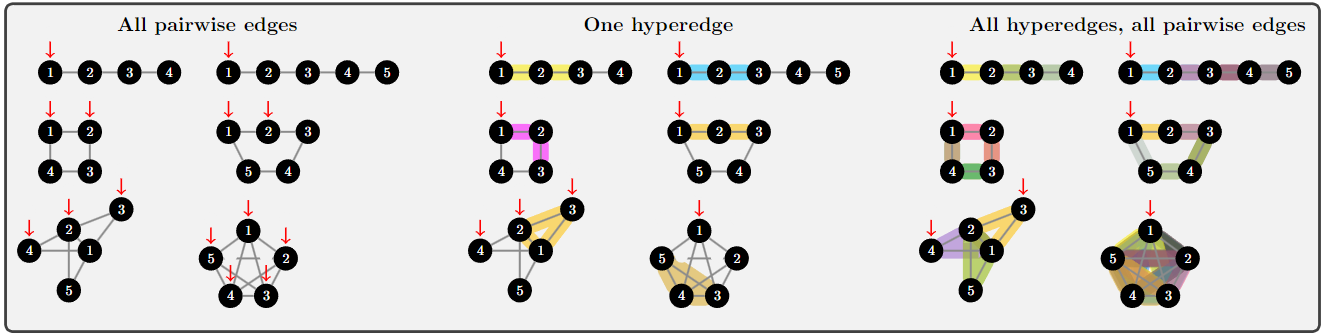
See Fig. 1 for an example of uniform hypergraph and associated dynamics. All the interactions are characterized using multiplications instead of the additions that are typically used in a standard graph based representation. For detailed discussion on relationship between graph vs. hypergraph dynamic representation, see Chen et al. (2021); Pickard, Chen, et al. (2023).

123$\dot{\textbf{x}}$=Ax$\Large\begin{cases}\dot{x}_{1}=x_{2}+x_{3}\\ \dot{x}_{2}=x_{1}+x_{3}\\ \dot{x}_{3}=x_{1}+x_{2}\end{cases}$A123$\dot{\textbf{x}}$=$\textsf{A}\textbf{x}^{2}$ $\Large\begin{cases}\dot{x}_{1}=x_{2}x_{3}\\ \dot{x}_{2}=x_{1}x_{3}\\ \dot{x}_{3}=x_{1}x_{2}\end{cases}$B
Figure 1: Graphs versus uniform hypergraphs. (A) Standard graph with three nodes and edges $e_{1}=\{1,2\}$, $e_{2}=\{2,3\}$ and $e_{3}=\{1,3\}$, and its corresponding linear dynamics. (B) 3-uniform hypergraph with three nodes and a hyperedge $e_{1}=\{1,2,3\}$, and its corresponding nonlinear dynamics.

4 NON-UNIFORM HYPERGRAPHS

In this section, we recast the homogeneous polynomial/multilinear hypergraph dynamical system in terms of the Kronecker product and derive a construction of the corresponding nonlinear observability matrix.

4.1 Non-Uniform Hypergraph

A nonuniform hypergraph allows hyperedges to contain any number of vertices, relaxing the constraint of hyperedge uniformity. The adjacency structure for nonuniform hypergraphs can be represented as a series of adjacency tensors for each set of uniformly sized hyperedges.

Definition 12

Let $\mathcal{G}=\{\mathcal{V},\mathcal{E}\}$ be a non-uniform hypergraph with $n=|\mathcal{V}|$ nodes and maximum edge cardinality $K$. For each edge cardinality $k=2,\cdots,K$ we can associate an adjacency tensor

$$\textsf{A}_{k}\in\mathbb{R}^{n\times n\times\dots\times n},$$

which is a $k$-th order, $n$-dimensional, supersymmetric tensor which captures all $k$-th order hyperedge interactions. Then $\mathcal{G}$ can be described by a collection of adjacency tensors $\{\textsf{A}_{k}\}_{k=2}^{K}$.

4.2 Nonuniform Hypergraph Dynamics with Outputs

Definition 13

Given a $K$-nonuniform undirected hypergraph $\mathcal{G}$ with $n$ nodes, the dynamics of $\mathcal{G}$ with outputs $\mathbf{y}\in\mathbb{R}^{m}$ is defined as

$$\Sigma\begin{cases}\dot{\mathbf{x}}&=\mathbf{f}(\mathbf{x})=\sum_{k=2}^{K}\textsf{A}_{k}\mathbf{x}^{k-1},\\ \mathbf{y}&=\mathbf{g}(\mathbf{x})=\mathbf{C}\mathbf{x},\end{cases}$$ (5)

where $\textsf{A}_{k}\in\mathbb{R}^{n\times n\times\dots\times n}$ is the adjacency tensors of $\mathcal{G}$, and $\mathbf{C}\in\mathbb{R}^{m\times n}$ is the output matrix.

The nonuniform hypergraph dynamics (5) can be expressed equivalently as the unfolded tensor A contracted with the Kronecker exponentiation of the state vector:

$$\Sigma\begin{cases}\dot{\mathbf{x}}&=\mathbf{f}(\mathbf{x})=\sum_{k=2}^{K}\mathbf{A}_{k}\mathbf{x}^{[k-1]},\\ \mathbf{y}&=\mathbf{g}(\mathbf{x})=\mathbf{C}\mathbf{x},\end{cases}$$ (6)

where, $\mathbf{A}_{k}=\textsf{A}_{k(p)}\in\mathbb{R}^{n\times n^{k-1}}$ is the $p$-th mode unfolding of $\textsf{A}_{k}$, and $\mathbf{x}^{[k]}=\mathbf{x}\otimes\mathbf{x}\cdots\otimes\mathbf{x}$ with $\otimes$ being the Kronecker product. Since $\textsf{A}_{k}$ is a super-symmetric tensor, all $p$-th mode unfoldings give rise to the same matrix.

Tensor unfoldings: Tensor unfolding is a fundamental operation in tensor computations Kolda and Bader (2009). In order to unfold a tensor $\textsf{T}\in\mathbb{R}^{n_{1}\times\cdots\times n_{k}}$ into a vector or a matrix, we use an index mapping function $ivec(\cdot,\mathcal{N}):\mathbb{Z}\times\mathbb{Z}\times\stackrel{{\scriptstyle\scriptscriptstyle k}}{{\cdots}}\times\mathbb{Z}\rightarrow\mathbb{Z}$, which is defined as

$$ivec(\mathcal{J},\mathcal{N})=j_{1}+\sum_{i=2}^{k}(j_{i}-1)\prod_{l=1}^{i-1}n_{l},$$

where $\mathcal{J}=\{j_{1},j_{2},\cdots,j_{k}\}$ and $\mathcal{N}=\{n_{1},\cdots,n_{k}\}$ are the sets of indices and mode sizes of T, respectively. The function $ivec$ is an injective map from the set of the tensor indices $\{j_{1},j_{2},\cdots,j_{k}\}$ to a unique vector index and is used to unfold or matricize tensors.

Tensor $p$-mode unfolding Kolda and Bader (2009): Given a $k$th-order tensor $\textsf{T}\in\mathbb{R}^{n_{1}\times\dots\times n_{k}}$, the $p$-mode unfolding of T, denoted by $\textsf{T}_{(p)}\in\mathbb{R}^{n_{p}\times(n_{1}\cdots n_{p-1}n_{p+1}\cdots n_{k})}$, is defined as

$$(\textsf{T}_{(p)})_{ij}=\textsf{T}_{j_{1}\cdots j_{p-1}ij_{p+1}\cdots j_{k}},$$

where $j=ivec(\tilde{\mathcal{J}},\tilde{\mathcal{N})}$ with $\tilde{\mathcal{J}}=\mathcal{J}\backslash\{j_{p}\}$ and $\tilde{\mathcal{N}}=\mathcal{N}\backslash\{n_{p}\}$.

4.3 Observability Criterion

To determine the nonlinear observabilty matrix (2) for the systems (5) and (6), we compute the Lie derivatives of the system output along the flow $\mathbf{f}$ of the system state, which can be decomposed as:

$$\mathbf{f}(\mathbf{x})=\sum_{k=2}^{K}\mathbf{f}_{k}(\mathbf{x}),$$

where, $\mathbf{f}_{k}=\mathbf{A}_{k}\mathbf{x}^{[k-1]}$. Also note that

$$L_{\mathbf{f}}\mathbf{g}(\mathbf{x})=L_{\sum_{k_{1}=2}^{K}\mathbf{f}_{k_{1}}}\mathbf{g}(\mathbf{x})=\sum_{k_{1}=2}^{K}L_{\mathbf{f}_{k_{1}}}\mathbf{g}(\mathbf{x}).$$

and

$$L^{2}_{\mathbf{f}}\mathbf{g}(\mathbf{x})=\sum_{k_{1}=2}^{K}\sum_{k_{2}=2}^{K}L_{\mathbf{f}_{k_{2}}}(L_{\mathbf{f}_{k_{1}}}\mathbf{g}(\mathbf{x})),$$

and, hence,

$$L^{n}_{\mathbf{f}}\mathbf{g}(\mathbf{x})=\sum_{k_{1}=2}^{K}\sum_{k_{2}=2}^{K}\cdots\sum_{k_{n}=2}^{K}L_{\mathbf{f}_{k_{n}}}\cdots L_{\mathbf{f}_{k_{2}}}L_{\mathbf{f}_{k_{1}}}\mathbf{g}(\mathbf{x}).$$

For each $\mathbf{f}_{k}$ one can show (time derivatives here are along the appropriate vector fields),

$\displaystyle L_{\mathbf{f}_{k}}^{0}\mathbf{g}(\mathbf{x})$ $\displaystyle=$ $\displaystyle\mathbf{C}\mathbf{x},$
$\displaystyle L_{\mathbf{f}_{k}}^{1}\mathbf{g}(\mathbf{x})$ $\displaystyle=$ $\displaystyle\frac{d}{dt}\mathbf{C}\mathbf{x}=\mathbf{C}\mathbf{A}_{k}\mathbf{x}^{[k-1]},$
$\displaystyle L_{\mathbf{f}_{k}}^{2}\mathbf{g}(\mathbf{x})$ $\displaystyle=$ $\displaystyle\frac{d}{dt}\mathbf{C}\mathbf{A}_{k}\mathbf{x}^{[k-1]}$
$\displaystyle=$ $\displaystyle\mathbf{C}\mathbf{A}_{k}\overline{\mathbf{B}}_{k2}\mathbf{x}^{2k-3},$
$\displaystyle\vdots$
$\displaystyle L_{\mathbf{f}_{k}}^{n}\mathbf{g}(\mathbf{x})$ $\displaystyle=$ $\displaystyle\mathbf{C}\mathbf{A}_{k}\overline{\mathbf{B}}_{k2}\dots\overline{\mathbf{B}}_{kn}\mathbf{x}^{[nk-(2n-1)]}\quad\forall n>2,$

where $\overline{\mathbf{B}}_{kp}$ is given by

$$\overline{\mathbf{B}}_{kp}=\sum_{i=1}^{(p-1)k-(2p-3)}\overbrace{\mathbf{I}\otimes\dots\otimes\overbrace{\mathbf{A}_{k}}^{i\text{-th pos.}}\otimes\dots\otimes\mathbf{I}}^{(p-1)k-(2p-3)\text{times}}.$$ (7)

On the other hand, for mixed terms,

$\displaystyle L_{\mathbf{f}_{k_{2}}}L_{\mathbf{f}_{k_{1}}}\mathbf{g}(\mathbf{x})$ $\displaystyle=$ $\displaystyle\frac{d}{dt}\mathbf{C}\mathbf{A}_{k_{1}}\mathbf{x}^{[{k_{1}}-1]}$
$\displaystyle=$ $\displaystyle\mathbf{C}\mathbf{A}_{k_{1}}\frac{d}{dt}\bigg{(}\overbrace{\mathbf{x}\otimes\mathbf{x}\dots\otimes\mathbf{x}}^{\text{$k_{1}-1$ times}}\bigg{)}$
$\displaystyle=$ $\displaystyle\mathbf{C}\mathbf{A}_{k_{1}}\bigg{(}\dot{\mathbf{x}}\otimes\dots\otimes\mathbf{x}+\cdots+\mathbf{x}\otimes\dots\otimes\dot{\mathbf{x}}\bigg{)}$
$\displaystyle=$ $\displaystyle\mathbf{C}\mathbf{A}_{k_{1}}\bigg{(}\sum\mathbf{x}\otimes\dots\otimes\mathbf{A}_{k_{2}}\mathbf{x}^{[k_{2}-1]}\otimes\dots\otimes\mathbf{x}\bigg{)}$
$\displaystyle=$ $\displaystyle\mathbf{C}\mathbf{A}_{k_{1}}\bigg{[}\bigg{(}\sum\mathbf{I}\otimes\dots\mathbf{A}_{k_{2}}\otimes\dots\mathbf{I}\bigg{)}\mathbf{x}^{[k_{2}+k_{1}-3]}\bigg{]}$
$\displaystyle=$ $\displaystyle\mathbf{C}\mathbf{A}_{k_{1}}\mathbf{B}_{k_{2}k_{1}}\mathbf{x}^{[k_{1}+k_{2}-3]},$

where,

$$\mathbf{B}_{k_{2}k_{1}}=\sum_{i=1}^{k_{1}-1}\overbrace{\mathbf{I}\otimes\dots\otimes\overbrace{\mathbf{A}_{k_{2}}}^{i\text{-th pos.}}\otimes\dots\otimes\mathbf{I}}^{k_{1}-1\text{times}}.$$ (8)

Similarly,

$\displaystyle L_{\mathbf{f}_{k_{3}}}L_{\mathbf{f}_{k_{2}}}L_{\mathbf{f}_{k_{1}}}\mathbf{g}(\mathbf{x})$ $\displaystyle=$ $\displaystyle\mathbf{C}\mathbf{A}_{k_{1}}\mathbf{B}_{k_{2}k_{1}}\mathbf{B}_{k_{3}k_{2}k_{1}}\mathbf{x}^{[k_{1}+k_{2}+k_{3}-5]},$

where,

$$\mathbf{B}_{k_{3}k_{2}k_{1}}=\sum_{i=1}^{k_{1}+k_{2}-3}\overbrace{\mathbf{I}\otimes\dots\otimes\overbrace{\mathbf{A}_{k_{3}}}^{i\text{-th pos.}}\otimes\dots\otimes\mathbf{I}}^{k_{1}+k_{2}-3\text{times}}.$$ (9)

Thus, in general,

$\displaystyle L_{\mathbf{f}_{k_{n}}}\cdots L_{\mathbf{f}_{k_{3}}}L_{\mathbf{f}_{k_{2}}}L_{\mathbf{f}_{k_{1}}}\mathbf{g}(\mathbf{x})$
$\displaystyle=$ $\displaystyle\mathbf{C}\mathbf{A}_{k_{1}}\mathbf{B}_{k_{2}k_{1}}\mathbf{B}_{k_{3}k_{2}k_{1}}\cdots\mathbf{B}_{k_{n}\cdots k_{3}k_{2}k_{1}}\mathbf{x}^{[\sum_{i=1}^{n}k_{i}-(2n-1)]},$

with,

$$\mathbf{B}_{k_{n}\cdots k_{3}k_{2}k_{1}}=\sum_{i=1}^{\sum_{i=1}^{n-1}k_{i}-(2n-3)}\overbrace{\mathbf{I}\otimes\dots\otimes\overbrace{\mathbf{A}_{k_{n}}}^{i\text{-th pos.}}\otimes\dots\otimes\mathbf{I}}^{\sum_{i=1}^{n-1}k_{i}-(2n-3)\text{times}}.$$

Note that if $n=p$ and $k_{1}=k_{2}=\cdots k_{p}=k$, i.e., the uniform hypergraph case, then

$\displaystyle\mathbf{B}_{\underbrace{k\cdots kkk}_{p-\text{times}}}$ $\displaystyle=$ $\displaystyle\sum_{i=1}^{\sum_{i=1}^{p-1}k-(2p-3)}\overbrace{\mathbf{I}\otimes\dots\otimes\overbrace{\mathbf{A}_{k}}^{i\text{-th pos.}}\otimes\dots\otimes\mathbf{I}}^{\sum_{i=1}^{p-1}k-(2p-3)\text{times}}$
$\displaystyle=$ $\displaystyle\sum_{i=1}^{(p-1)k-(2p-3)}\overbrace{\mathbf{I}\otimes\dots\otimes\overbrace{\mathbf{A}_{k}}^{i\text{-th pos.}}\otimes\dots\otimes\mathbf{I}}^{(p-1)k-(2p-3)\text{times}},$

reduces to the matrix (see Pickard, Surana, et al. (2023)) which arise in calculating NOM for uniform hypergraph case as expected.

Finally,

$\displaystyle L^{n}_{\mathbf{f}}\mathbf{g}(\mathbf{x})=\sum_{k_{1}=2}^{K}\sum_{k_{2}=2}^{K}\cdots\sum_{k_{n}=2}^{K}\mathbf{C}\mathbf{A}_{k_{1}}$
$\displaystyle\mathbf{B}_{k_{2}k_{1}}\mathbf{B}_{k_{3}k_{2}k_{1}}\cdots\mathbf{B}_{k_{n}\cdots k_{3}k_{2}k_{1}}\mathbf{x}^{[\sum_{i=1}^{n}k_{i}-(2n-1)]},$

and we can express the NOM as,

$$\mathcal{O}(\mathbf{x})=\nabla_{\mathbf{x}}\begin{pmatrix}\mathbf{C}\mathbf{x}\\ \sum_{k_{1}=2}^{K}\mathbf{C}\mathbf{A}_{k_{1}}\mathbf{x}^{k_{1}-1}\\ \sum_{k_{1}=2}^{K}\sum_{k_{2}=2}^{K}\mathbf{C}\mathbf{A}_{k_{1}}\mathbf{B}_{k_{2}k_{1}}\mathbf{x}^{[k_{1}+k_{2}-3]}\\ \\ \vdots\\ L^{n}_{\mathbf{f}}\mathbf{g}\end{pmatrix},$$ (10)

where, we have used $r=n$ as per the Remark 2. From Theorem 1, when $\mbox{rank}(\mathcal{O}(\mathbf{x}))=\dim(\mathbf{x}),$ systems (5) and equivalently (6) are observable.

Refer to caption
Figure 2: (Left) Hypergraphs containing only pairwise edges are shown. Red arrows indicate a MON (minimum observable note) set to render each structure localy weakly observable. The top row contains two hyperchains, the middle row is two hyperrings, the bottom row contains the clique expansion of a uniform hyperstar and a complete hypergraph. (Middle) A single 3-way hyperedge has been added to each of the 2-uniform hypergraphs on the left, improving the observability of all hypergraphs. (Right) All 3-way hyperedges have been added to the hyperchain, hyperring, hyperstar and complete hypergraphs while still including the pairwise structure. c.f Pickard, Surana, et al. (2023) for the MON on similar 3-uniform hypergraphs.
Property 1

Given a nonuniform hypergraph $\mathcal{G}$ with a maximum hyperedge cardinality of $k,$ if $\mathcal{G}$ is locally weakly observable when all hyperedges with cardinality less than $k$ are removed, then $\mathcal{G}$ is locally weakly observable.

Proof. Consider a $k$-uniform hypergraph $\mathcal{G}$ that is locally weakly observable such that the symbolic NOM $\mathcal{O}(\mathbf{x})$ is of full rank. The inclusion of a hyperedge with cardinality less than $k$ in $\mathcal{G}$ will introduce polynomial terms of $\mathbf{x}$ into the symbolic NOM; however, the highest order polynomial terms in the NOM are generated by hyperedges of maximum cardinality, such that lower order polynomial terms cannot decrease the symbolic rank. Since hyperedges of lower cardinality introduce lower order polynomial terms into $\mathcal{O}(\mathbf{x}),$ the inclusion of hyperedges with fewer than $k$ vertices cannot decrease the symbolic rank of the hypergraph with only $k$-way hyperedges. $\blacksquare$

In Fig. 2, several hypergraph topologies are drawn with the minimum observable nodes (MON) required to make the hypergraphs observable. The number of 2-uniform hyperedges is fixed, and the number of 3-uniform hyperedges varies. We utilized the greedy selection procedure of Pickard, Surana, et al. (2023), where only 3-uniform hypergraphs were considered, to draw Fig 2. Consistent with Proposition 15, the increase in hyperedges uniformly decreases the size of the MON, which further motivates the investigation of higher order observability.

5 Conclusion

We have analyzed observability for non-uniform hypergraphs, applying the theory developed earlier for the uniform case, and illustrated the work on several low-dimensional examples. Future work will include applying these ideas to large data sets, particularly those arising from biological applications.

Acknowledgement: We would like to thank the reviewers for very helpful comments regarding the exposition.

References

  • \NAT@swatrue
  • Anguelova (2004) Anguelova, M.  (2004). Nonlinear observability and identi ability: General theory and a case study of a kinetic model for s. cerevisiae. Chalmers Tekniska Hogskola (Sweden). \NAT@swatrue
  • Baillieul (1981) Baillieul, J.  (1981). Controllability and observability of polynomial dynamical systems. Nonlinear Analysis: Theory, Methods & Applications, 5(5), 543–552. \NAT@swatrue
  • Chen et al. (2021) Chen, C., Surana, A., Bloch, A., and Rajapakse, I.  (2021). Controllability of hypergraphs. IEEE Transactions on Network Science and Engineering. \NAT@swatrue
  • Gerbet and Röbenack (2020) Gerbet, D., and Röbenack, K.  (2020). On global and local observability of nonlinear polynomial systems: A decidable criterion. at-Automatisierungstechnik, 68(6), 395–409. \NAT@swatrue
  • Hermann and Krener (1977) Hermann, R., and Krener, A.  (1977). Nonlinear controllability and observability. IEEE Transactions on automatic control, 22(5), 728–740. \NAT@swatrue
  • Kolda and Bader (2009) Kolda, T. G., and Bader, B. W.  (2009). Tensor decompositions and applications. SIAM review, 51(3), 455–500. \NAT@swatrue
  • Lin (1974) Lin, C.-T.  (1974). Structural controllability. IEEE Transactions on Automatic Control, 19(3), 201–208. \NAT@swatrue
  • Liu et al. (2013) Liu, Y.-Y., Slotine, J.-J., and Barabási, A.-L.  (2013). Observability of complex systems. Proceedings of the National Academy of Sciences, 110(7), 2460–2465. \NAT@swatrue
  • A. Montanari and Aguirre (2019) Montanari, A., and Aguirre, L. A.  (2019). Particle filtering of dynamical networks: Highlighting observability issues. Chaos: An Interdisciplinary Journal of Nonlinear Science, 29(3), 033118. \NAT@swatrue
  • A. N. Montanari and Aguirre (2020) Montanari, A. N., and Aguirre, L. A.  (2020). Observability of network systems: A critical review of recent results. Journal of Control, Automation and Electrical Systems, 31, 1348–1374. \NAT@swatrue
  • Pickard, Chen, et al. (2023) Pickard, J., Chen, C., Stansbury, C., Surana, A., Bloch, A., and Rajapakse, I.  (2023). Kronecker product of tensors and hypergraphs: structure and dynamics. arXiv preprint arXiv:2305.03875. \NAT@swatrue
  • Pickard, Surana, et al. (2023) Pickard, J., Surana, A., Bloch, A., and Rajapakse, I.  (2023). Observability of hypergraphs. Proceedings of the 2023 CDC. \NAT@swatrue
  • Sedoglavic (2001) Sedoglavic, A.  (2001). A probabilistic algorithm to test local algebraic observability in polynomial time. In Proceedings of the 2001 international symposium on symbolic and algebraic computation (pp. 309–317). \NAT@swatrue
  • Sontag (1984) Sontag, E. D.  (1984). A concept of local observability. Systems & Control Letters, 5(1), 41–47. \NAT@swatrue
  • Su et al. (2017) Su, F., Wang, J., Li, H., Deng, B., Yu, H., and Liu, C.  (2017). Analysis and application of neuronal network controllability and observability. Chaos: An Interdisciplinary Journal of Nonlinear Science, 27(2), 023103. \NAT@swatrue
  • Summers and Lygeros (2014) Summers, T. H., and Lygeros, J.  (2014). Optimal sensor and actuator placement in complex dynamical networks. IFAC Proceedings Volumes, 47(3), 3784–3789.