Cramér-Rao Bounds for Near-Field Sensing: A Generic Modular Architecture

Abstract

A generic modular array architecture is proposed, featuring uniform/non-uniform subarray layouts that allows for flexible deployment. The bistatic near-field sensing system is considered, where the target is located in the near-field of the whole modular array and the far-field of each subarray. Then, the closed-form expressions of Cramér-Rao bounds (CRBs) for range and angle estimations are derived based on the hybrid spherical and planar wave model (HSPM). Simulation results validate the accuracy of the derived closed-form CRBs and demonstrate that: i) The HSPM with varying angles of arrival (AoAs) between subarrays can reduce the CRB for range estimation compared to the traditional HSPM with shared AoA; and ii) The proposed generic modular architecture with subarrays positioned closer to the edges can significantly reduce the CRBs compared to the traditional modular architecture with uniform subarray layout, when the array aperture is fixed.

I Introduction

In the sixth generation wireless systems, the extremely large-scale (XL) antenna arrays and millimeter wave (mmWave)/terahertz (THz) are considered key technologies to significantly enhance the spectrum efficiency and spatial resolution, which is essential to meet the demands for high-capacity communications and high-resolution sensing of emerging applications such as smart manufacturing and smart home[1, 2]. Nevertheless, the larger array apertures and higher frequency bands will result in communication users or sensing targets being located in the near-field region, rendering the traditional far-field channel model based on planar electromagnetic wavefront invalid[3]. Therefore, it is necessary to consider more general spherical wavefront characteristics for both near-field communications and sensing.

Recently, the modular XL-array has been regarded as a promosing architecture utilized for the mmWave/THz frequency bands, which is comprised of multiple identical subarrays with uniform array antennas and relatively large intervals between adjacent subarrays[3, 4, 5]. The modular XL-array with a larger array aperture enables an extended near-field range, improved spatial resolution, and flexible deployment[6]. Therefore, [7] investigated the potential of modular XL-arrays in near-field sensing and conducted a detailed analysis of the range and angle Cramér-Rao Bound (CRB)s. However, the studies mentioned above considered the modular XL-array with uniformly arranged subarrays, which can result in unignorable grating lobes[5]. In [8], a novel approach is proposed based on a non-uniform subarray layout to suppress the sidelobes of the modular XL-array and enable ambiguity-free angle of arrival (AoA) estimation. The aurthors in [9] derived CRBs based on spherical-wave model (SWM) with antenna arrays of arbitrary geometry. However, in a modular architecture, due to the smaller subarray aperture compared to the entire array aperture, the target is more likely to be located in the near-field of the entire array and the far-field of each subarray[4]. Therefore, employing the hybrid spherical and planar wave model (HSPM) is more suitable due to its advantages in low modeling and computational complexity over the SWM.

In this letter, we propose a novel generic modular array architecture with uniform/non-uniform subarray arrangement and investigate its potential in near-field sensing. We consider a bistatic near-field sensing system operating in the phased-array radar mode. Additionally, we derive closed-form expressions of the range and angle CRBs based on the HSPM model, considering varying subarray AoAs. Simulation results demonstrate that: 1) The HSPM with distinct AoAs yields significantly lower range CRB compared to the commonly used HSPM with shared AoA, and closely approximates the SWM in terms of the range and angle CRBs. 2) In a centro-symmetric modular array with a fixed aperture, a non-uniform arrangement of subarrays near the edges achieves lower range and angle CRBs than a traditional uniform subarray arrangement. This validates the effectiveness of the proposed generic modular array architecture in near-field sensing.

II System Model

We consider a bistatic near-field sensing system as illustrated in Fig. 1, with application scenarios including unmanned aerial vehicles surveillance and assisted driving in intelligent transportation systems[10, 11]. The transmitter (Tx) is equipped with a uniform XL-array comprising $N_{t}$ antennas. The receiver (Rx) is equipped with a generic modular XL-array incorporating $N_{r}=KM$ antennas, where $K$ is the number of subarrays and $M$ is the number of antenna elements within each subarray. The distance between the centers of Tx and Rx is $R$. The inter-antenna spacing of Tx/Rx is denoted as $d=\frac{\lambda}{2}$, where $\lambda$ denotes the wavelength. For notational convinience, we assume that $N_{t}$, $K$, and $M$ are odd numbers, so that the $n$-th antenna at Tx, the $k$-th subarray at Rx, and $m$-th antenna of each subarray belong to the integer sets $\mathcal{N}={\left\{0,\pm 1,\cdots,\pm\frac{N_{t}-1}{2}\right\}}$, $\mathcal{K}={\left\{0,\pm 1,\cdots,\pm\frac{K-1}{2}\right\}}$, and $\mathcal{M}={\left\{0,\pm 1,\cdots,\pm\frac{M-1}{2}\right\}}$, respectively.

Without loss of generality, we assume that the generic modular XL-array of Rx is placed along the $x$-axis, while the Tx array is oriented at an angle $\delta$ with respect to the Rx array. For each subarray, we select its center element as the reference antenna. The distance between the k-th subarray and its adjacent subarray closer to the origin is $\Gamma_{k}d$, where $\Gamma_{k}\geq 1$ is an integer determined by the practical deployment conditions. Therefore, the coordinate of the $m$-th element of the $k$-th subarray can be represented as $\mathbf{l}_{k,m}=(x_{k,m},0)$, where $x_{k,m}=(\sum\nolimits_{i=0}^{k}{{{\Gamma}_{i}}}+k(M-1)+m)d$ for $k>0$, and $x_{k,m}=(-\sum\nolimits_{i=0}^{k}{{{\Gamma}_{i}}}+k(M-1)+m)d$ for $k\leq 0$.

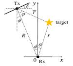
Figure 1: Illustration of the bistatic near-field sensing system.

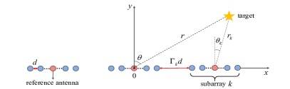
Figure 2: The generic modular array with $K$ subarrays and $M$ antennas in each subarray.

The radar target is located at $\mathbf{l}_{q}=(r\sin\theta,r\cos\theta)$, where $r$ is its distance from the origin, and $\theta\in\left[-\frac{\pi}{2},\frac{\pi}{2}\right]$ is its angle with respect to the positive $y$-axis. Let $\varphi$, $\phi$, and $\bar{r}$ denote the AoA, the relative angle, and distance between the target and the center of Tx array, respectively. With prior knowledge about the relative positions of Tx and Rx, specifically the known parameters $R$, $\phi$, and $\delta$, distance $\bar{r}$ and angle $\varphi$ at Tx can be expressed in terms of the parameters $r$ and $\theta$ at Rx, namely,

$$\bar{r}(r,\theta)=\sqrt{{{R}^{2}}+{{r}^{2}}-2Rr\cos(\theta+\phi)},$$ (1)

$$\varphi(r,\theta)=\arcsin\left\{\frac{r\sin\theta+R\sin\phi}{\sqrt{{{R}^{2}}+{{r}^{2}}-2Rr\cos(\theta+\phi)}}\right\}.$$

In cases where $\bar{r}\leq\frac{2[(N_{t}-1)d]^{2}}{\lambda}$, the transmit array response vector based on SWM is given by ${\mathbf{g}_{t}}(r,\theta)={{[e{{}^{-j\frac{2\pi}{\lambda}\bar{r}_{n}}}]}_{\forall n\in\mathcal{N}}}$, with $\bar{r}_{n}=\sqrt{{\bar{r}}^{2}-2\bar{r}nd\sin(\varphi-\delta)+(nd)^{2}}$.

Note that the large inter-subarray spacing of Rx, i.e., $\Gamma_{k}d$, results in an expanded array aperture, which is given by $S=(\sum\nolimits_{k\in\mathcal{K}}{{{\Gamma}_{i}}}+K(M-1))d$. When $\frac{2[(M-1)d]^{2}}{\lambda}\leq r\leq\frac{2S^{2}}{\lambda}$, the target is located in the near-field of the entire array and the far-field of individual subarrays. Then, the HSPM becomes applicable by combining spherical wave propagation between subarrays and planar wave propagation for each subarray[4, 12]. Specifically, the distance between the target and the reference antenna of the $k$-th subarray in Rx can be expressed as

$$r_{k}=\left\|\mathbf{l}_{q}-\mathbf{l}_{k,0}\right\|=\sqrt{r^{2}-2rx_{k}\sin\theta+(x_{k})^{2}},$$ (2)

where $x_{k}\triangleq x_{k,0}$ denotes the abscissa cooridnate of the $k$-th subarray’s reference antenna. By utilizing the HSPM with distinct AoAs[5], the Rx array response vectors can be obtained as

$${{\mathbf{g}}_{r}}=\left(\text{diag}\left({{\bm{\nu}}}\right)\otimes{{\mathbf{I}}_{M}}\right){{{\mathbf{\tilde{a}}}}},$$ (3)

where ${{\bm{\nu}}}={{[e{{}^{-j\frac{2\pi}{\lambda}r_{k}}}]}_{\forall k\in\mathcal{K}}}$ represents the inter-subarray response vector under the uniform spherical-wave assumption, ${{\mathbf{\tilde{a}}}}={{[{{(\mathbf{a}_{1})}^{T}},\ldots,{{(\mathbf{a}_{K})}^{T}}]}^{T}}\in\mathbb{C}^{KM\times 1}$ with ${{\mathbf{a}}_{k}}={{[{{e}^{j\frac{2\pi}{\lambda}\frac{(M-1)}{2}d\sin{{\theta}_{k}}}},\ldots,{{e}^{-j\frac{2\pi}{\lambda}\frac{(M-1)}{2}d\sin{{\theta}_{k}}}}]}^{T}},\forall k\in\mathcal{K}$ denotes the intra-subarray response vectors under the uniform planar-wave assumption. The angle of target observed from the $k$-th subarray’s reference antenna is denoted as ${\theta}_{k}$, which can be obtained as

$$\sin\theta_{k}=\frac{r\sin\theta-{{x}_{k}}}{\sqrt{r^{2}-2rx_{k}\sin\theta+(x_{k})^{2}}}.$$ (4)

In order to track the target at a specific position, the Tx operates in a phased-array radar mode, generating the transmit beam towards the specific distance $r^{\prime}$ and angle ${\theta}^{\prime}$. Within the coherent processing interval, the target is assumed to be stationary. Consequently, the narrow-band transmitted signal is given by

$$\mathbf{x}\left(t\right)=\mathbf{w}_{t}s\left(t\right),$$ (5)

where $\mathbf{w}_{t}=\mathbf{g}_{t}^{*}(\bar{r},\phi-\delta)\in\mathbb{C}^{N_{t}\times 1}$ is the transmit beamfocusing vector towards the target at the position $(\bar{r},\phi-\delta)$ in the Tx-centric coordinate system, which corresponds to the target position $(r^{\prime},\theta^{\prime})$ in the Rx-centric coordinate system, and $s(t)$ represents the transmitted waveform. The Rx employs fast-time sampling within each pulse to obtain the received signal. Therefore, the received signal for bistatic near-field sensing is

$$\mathbf{r}\left(t\right)=\beta{{\mathbf{g}}_{r}}\mathbf{g}_{t}^{T}\mathbf{x}\left(t-\tau\right)+\mathbf{n}\left(t\right),$$ (6)

where $\beta$ is the complex reflection coefficient proportional to the radar cross section (RCS) of the target, $\tau=\frac{\bar{r}+r}{c}$ is the round-trip time delay from the transmitter to the target and back to the center antenna of Rx, $c$ is the speed of light, and $\mathbf{n}(t)$ denotes the additive white Gaussian noise (AWGN), with each element being independent and identically distributed (i.i.d.) circularly symmetric complex Gaussian noise with power spectral density $\sigma_{s}^{2}$. Subsequently, by substituting (5) into (6) and performing matched filtering, we can obtain

$$\mathbf{y} =\frac{1}{T}\int_{T}{\mathbf{r}}(t){{s}^{*}}(t-\zeta)dt$$ (7)

$$=\beta{{\mathbf{g}}_{r}}\mathbf{g}_{t}^{T}(r,\theta)\mathbf{g}_{t}^{*}\left({r}^{\prime},{\theta}^{\prime}\right)R\left(\zeta-\tau\right)+\mathbf{\tilde{n}},$$

where $R\left(\zeta-\tau\right)=\frac{1}{T}\int_{T}{s(t-\tau){{s}^{*}}(t-\zeta)}dt$ is the autocorrelation function, and $\mathbf{\tilde{n}}$ is the noise vector obtained after matched filtering, with zero mean and variance $\sigma_{s}^{2}$. When the parameters of both the matched filter and the transmit beamforming align with the true values of the target parameters, i.e., $r^{\prime}=r$, ${\theta}^{\prime}=\theta$, $\zeta=\tau$, the transmit beam can be focused towards the target, thereby achieving maximized signal-to-interference-plus-noise ratio (SINR) at Rx[13]. Therefore, the output of the received signal after matched filtering is given by

$$\mathbf{y}=\alpha\mathbf{g}_{r}+\mathbf{\tilde{n}},$$ (8)

where $\alpha\triangleq\beta N_{t}$ denotes the constant coefficient gain.

III Performance Analysis of Cramér-Rao Bound

Let $\bm{\eta}={{\left[r,\theta,{{\beta}_{r}},{{\beta}_{i}}\right]}^{T}}$ represent the vector that incorporates all unknown target-related parameters, with ${{\beta}_{r}}$ and ${{\beta}_{i}}$ denoting the real and imaginary parts of $\beta$, respectively. Since the spherical wavefront curvature contains two-dimensional angle and distance information, a direct positioning estimation method can be employed to extract the target’s position information from the received signal[14, 15]. In this letter, we use CRB to evaluate the performance of the target position estimation.

Following, we derive the closed-form CRBs of the generic modular XL-array under four different wavefront assumptions, namely: 1) HSPM with distinct AoAs, 2) HSPM with shared AoA, 3) planar-wave model (PWM) , and 4) SWM.

Theorem 1

The CRBs based on HSPM with distinct AoAs for estimating range and angle can be expressed as follows, respectively,

$$\text{CRB}_{r}^{\text{HSPM-Dist}}$$

$$=\frac{\frac{6\sigma_{s}^{2}K}{{{\left|\alpha\right|}^{2}}M}{{\left(\frac{\lambda}{2\pi}\right)}^{2}}}{K\!\left(\!{{M}^{2}}\!-\!1\!\right){{d}^{2}}z\!+\!12Kq\!-\!12{{p}^{2}}\!-\!\frac{{{\left[K\left({{M}^{2}}-1\right){{d}^{2}}\hat{z}+12K\hat{q}-12p\tilde{p}\right]}^{2}}}{K\left({{M}^{2}}-1\right){{d}^{2}}\tilde{z}+12K\tilde{q}-12{{{\tilde{p}}}^{2}}}},$$ (9a)

$$\text{CRB}_{\theta}^{\text{HSPM-Dist}}$$

$$=\frac{\frac{6\sigma_{s}^{2}K}{{{\left|\alpha\right|}^{2}}M}{{\left(\frac{\lambda}{2\pi}\right)}^{2}}}{K\!\left(\!{{M}^{2}}\!-\!1\!\right){{d}^{2}}\tilde{z}\!+\!12K\tilde{q}\!-\!12{{{\tilde{p}}}^{2}}\!-\!\frac{{{\left[K\left({{M}^{2}}-1\right){{d}^{2}}\hat{z}+12K\hat{q}-12p\tilde{p}\right]}^{2}}}{K\left({{M}^{2}}-1\right){{d}^{2}}z+12Kq-12{{p}^{2}}}},$$ (9b)

where $p\triangleq\sum\nolimits_{k\in\mathcal{K}}{\frac{\partial{{r}_{k}}}{\partial r}}$, $\tilde{p}\triangleq\sum\nolimits_{k\in\mathcal{K}}{\frac{\partial{{r}_{k}}}{\partial\theta}}$, $q\triangleq{{\sum\nolimits_{k\in\mathcal{K}}{\left(\frac{\partial{{r}_{k}}}{\partial r}\right)}}^{2}}$, $\tilde{q}\triangleq\sum\nolimits_{k\in\mathcal{K}}{{{\left(\frac{\partial{{r}_{k}}}{\partial\theta}\right)}^{2}}}$, $\hat{q}\triangleq\sum\nolimits_{k\in\mathcal{K}}{\left(\frac{\partial{{r}_{k}}}{\partial r}\right)\left(\frac{\partial{{r}_{k}}}{\partial\theta}\right)}$, $z\triangleq\sum\nolimits_{k\in\mathcal{K}}{{{\left(\frac{\partial\sin{{\theta}_{k}}}{\partial r}\right)}^{2}}}$, $\tilde{z}\triangleq\sum\nolimits_{k\in\mathcal{K}}{{{\left(\frac{\partial\sin{{\theta}_{k}}}{\partial\theta}\right)}^{2}}}$, and$\hat{z}\triangleq\sum\nolimits_{k\in\mathcal{K}}{\left(\frac{\partial\sin{{\theta}_{k}}}{\partial r}\right)\left(\frac{\partial\sin{{\theta}_{k}}}{\partial\theta}\right)}$. The corresponding derivatives in the above expressions are given by

$$\frac{\partial{{r}_{k}}}{\partial r}\!\!=\!\!\frac{r-{{x}_{k}}\sin\theta}{\sqrt{{{r}^{2}}\!-\!2r{{x}_{k}}\sin\theta\!+\!{x}_{k}^{2}}},\frac{\partial\sin\!{\theta}_{k}}{\partial r}\!\!=\!\!\frac{r{{x}_{k}}{{\cos}^{2}}\theta}{{\left({{r}^{2}}\!-\!2r{{x}_{k}}\sin\theta\!+\!{x}_{k}^{2}\right)}^{\frac{3}{2}}},$$ (10)

$$\frac{\partial{{r}_{k}}}{\partial\theta}\!\!=\!\!\frac{-r{{x}_{k}}\cos\theta}{\sqrt{{{r}^{2}}\!-\!2r{{x}_{k}}\sin\theta\!+\!{x}_{k}^{2}}},\frac{\partial\sin\!{{\theta}_{k}}}{\partial\theta}\!\!=\!\!\frac{{{r}^{2}}\cos\theta\left(r\!-\!\sin\theta{{x}_{k}}\right)}{{\left({{r}^{2}}\!-\!2r{{x}_{k}}\sin\theta\!+\!{x}_{k}^{2}\right)}^{\frac{3}{2}}}.$$

Proof:

Please refer to Appendix A. ∎

From (9), we observe that the impact of different AoAs for each subarray on the CRBs manifests in $z$, $\tilde{z}$, and $\hat{z}$. It is also noted that both range and angle CRB expressions contain distance-angle coupling terms, which are characterized by the intermediate variables $\hat{z}$, $\hat{q}$, and $p\tilde{p}$. These coupling terms originate from the off-diagonal elements of the Fisher information matrix, indicating the correlation between the estimation of distance and angle parameters.

In contrast, for HSPM with shared AoA, the AoAs of different subarrays are considered approximately equal, i.e., $\sin\theta_{k}=\sin\theta,\forall k$, thus we have $z=0$, $\tilde{z}=K\cos^{2}\theta$, and $\hat{z}=0$. Consequently, we can readily derive the closed-form CRBs under the HSPM with shared AoA from Theorem 1, as follows.

Proposition 1

The CRBs based on HSPM with shared AoA for estimating range and angle can be derived as a degeneration of (9), which are expressed as follows, respectively,

$${\text{CRB}}_{r}^{\text{HSPM-Shared}}$$

$$=\frac{\frac{6\sigma_{s}^{2}K}{{{\left|\alpha\right|}^{2}}M}{{\left(\frac{\lambda}{2\pi}\right)}^{2}}}{\!12Kq\!-\!12{{p}^{2}}\!-\!\frac{{{\left[12K\hat{q}-12p\tilde{p}\right]}^{2}}}{K^{2}\left({{M}^{2}}-1\right){{d}^{2}}{(\cos\theta)}^{2}+12K\tilde{q}-12{{{\tilde{p}}}^{2}}}},$$ (11a)

$${\text{CRB}}_{\theta}^{\text{HSPM-Shared}}$$

$$=\!\!\frac{\frac{6\sigma_{s}^{2}K}{{{\left|\alpha\right|}^{2}}M}{{\left(\frac{\lambda}{2\pi}\right)}^{2}}}{K^{2}\!\left(\!{{M}^{2}}\!\!-\!\!1\!\right){{d}^{2}}{(\cos\theta)}^{2}\!\!+\!\!12K\tilde{q}\!\!-\!\!12{{{\tilde{p}}}^{2}}\!\!-\!\!\frac{{{\left[12K\hat{q}-12p\tilde{p}\right]}^{2}}}{12Kq-12{{p}^{2}}}}.$$ (11b)

From (11), we can observe that the coupling terms only consist of $\hat{q}$ and $p\tilde{p}$, indicating a weaker distance-angle coupling compared to the HSPM with distinct AoAs.

Subsequently, we can similarly obtain the CRBs of range and angle under the PWM as presented in the following proposition.

Proposition 2

The CRBs based on PWM for estimating range and angle can be expressed as follows, respectively,

$$\text{CRB}_{r}^{\text{PWM}} \rightarrow+\infty,$$ (12)

$$\text{CRB}_{\theta}^{\textit{PWM}} \!=\!\frac{\frac{6\sigma_{s}^{2}K}{{{\left|\alpha\right|}^{2}}{{\cos}^{2}}\theta}{{\left(\frac{\lambda}{2\pi}\right)}^{2}}}{12KM\!\sum\limits_{k\in\mathcal{K}}\!{x_{k}^{2}}\!+\!{{K}^{2}}M\left({{M}^{2}}\!-\!1\right){{d}^{2}}\!-\!12M{{(\sum\limits_{k\in\mathcal{K}}{{{x}_{k}}})}^{2}}}.$$

It is observed that the CRB of range in (12) tends towards infinity, as the antenna array is incapable of spatially discerning ranges under PWM assumption. Furthermore, the absence of distance-angle coupling terms in the angle CRB implies that the angle estimation performance is independent of $r$.

Then, building upon [16], we derive the CRBs based on the SWM which precisely captures the signal phase variations across all array elements.

Proposition 3

The CRBs based on SWM for estimating range and angle can be expressed as follows, respectively,

$$\text{CRB}_{r}^{\text{SWM}}=\frac{\frac{\sigma_{s}^{2}KM}{2{{\left|\alpha\right|}^{2}}}{{\left(\frac{\lambda}{2\pi}\right)}^{2}}}{KM{{\varpi}_{rr}}-{{\left({{\varpi}_{r}}\right)}^{2}}-\frac{{{\left(KM{{\varpi}_{r\theta}}-{{\varpi}_{r}}{{\varpi}_{\theta}}\right)}^{2}}}{KM{{\varpi}_{\theta\theta}}-{{\left({{\varpi}_{\theta}}\right)}^{2}}}},$$ (13a)

$$\text{CRB}_{\theta}^{\text{SWM}}=\frac{\frac{\sigma_{s}^{2}KM}{2{{\left|\alpha\right|}^{2}}}{{\left(\frac{\lambda}{2\pi}\right)}^{2}}}{KM{{\varpi}_{\theta\theta}}-{{\left({{\varpi}_{\theta}}\right)}^{2}}-\frac{{{\left(KM{{\varpi}_{r\theta}}-{{\varpi}_{r}}{{\varpi}_{\theta}}\right)}^{2}}}{KM{{\varpi}_{rr}}-{{\left({{\varpi}_{r}}\right)}^{2}}}},$$ (13b)

where ${{\varpi}_{r}}\!\triangleq\!\sum\limits_{k,m}{\frac{\partial{{r}_{k,m}}}{\partial r}}$, ${{\varpi}_{\theta}}\triangleq\sum\limits_{k,m}{}\frac{\partial{{r}_{k,m}}}{\partial\theta}$, ${{\varpi}_{rr}}\triangleq\sum\limits_{k,m}{}{{\left(\frac{\partial{{r}_{k,m}}}{\partial r}\right)}^{2}}$, ${{\varpi}_{r\theta}}\triangleq\sum\limits_{k,m}{\left(\frac{\partial{{r}_{k,m}}}{\partial r}\right)\left(\frac{\partial{{r}_{k,m}}}{\partial\theta}\right)}$, ${{\varpi}_{\theta\theta}}\triangleq\sum\limits_{k,m}{{{\left(\frac{\partial{{r}_{k,m}}}{\partial\theta}\right)}^{2}}}$.

Under the SWM assumption, the coupling terms present in both range and angle CRBs are characterized by ${\varpi}_{r\theta}$ and ${\varpi}r{\varpi}{\theta}$. Compared to the HSPM for distinct AoAs, the SWM exhibits stronger distance-angle coupling since it considers the unique distance of each antenna element, which inherently contains information about the distance and angle parameters.

In traditional estimation theory, coupling between parameters may degrade accuracy due to error propagation[17]. However, in near-field sensing, coupling terms determined by the target’s location and wavefront assumption can provide additional information for parameter estimation, thereby facilitating the joint estimation of range and angle[18].

To gain more intuitive insights, we consider a centro-symmetric array and the special case of $\theta=0$, i.e., the target is located on the y-axis. This eliminates the complex distance-angle coupling terms, yielding simplified CRB expressions, as elucidated in the following corollaries.

Corollary 1

When $\theta=0$, the CRBs in Theorem 1 reduce to

$$\text{CRB}_{r}^{\text{HSPM-Dist}}\!\!=\!\!\frac{\frac{6\sigma_{s}^{2}K}{{{\left|\alpha\right|}^{2}}M}{{\left(\frac{\lambda}{2\pi}\right)}^{2}}}{K\left({{M}^{2}}-1\right){{d}^{2}}{z}^{\prime}+12K{q}^{\prime}-12{{\left({{p}^{\prime}}\right)}^{2}}},$$ (14a)

$$\text{CRB}_{\theta}^{\text{HSPM-Dist}}\!\!=\!\!\frac{\frac{6\sigma_{s}^{2}}{{{\left|\alpha\right|}^{2}}}{{\left(\frac{\lambda}{2\pi}\right)}^{2}}}{M\left({{M}^{2}}-1\right){{d}^{2}}{\tilde{z}}^{\prime}+12M{\tilde{q}}^{\prime}},$$ (14b)

where ${p}^{\prime}\triangleq\sum\nolimits_{k\in\mathcal{K}}\frac{r}{r_{k}}$, ${q}^{\prime}\triangleq\sum\nolimits_{k\in\mathcal{K}}\frac{{{r}^{2}}}{{{r}_{k}^{2}}}$, ${z}^{\prime}\triangleq\sum\nolimits_{k\in\mathcal{K}}\frac{{{r}^{2}{x_{k}^{2}}}}{{{r}_{k}^{6}}}$, $\tilde{q}^{\prime}\triangleq\sum\nolimits_{k\in\mathcal{K}}\frac{{{r}^{2}{x_{k}^{2}}}}{{{r}_{k}^{2}}}$, $\tilde{z}^{\prime}\triangleq\sum\nolimits_{k\in\mathcal{K}}\frac{r^{6}}{{{r}_{k}^{6}}}$, with ${{r}_{k}}=\sqrt{{{r}^{2}}+{{x}_{k}^{2}}},\forall k\in\mathcal{K}$.

Proof:

Please refer to Appendix B. ∎

It can be easily observed from Corollary 1 that as $r$ increases, both $\tilde{z}^{\prime}$ and $\tilde{q}^{\prime}$ increase, leading to a decrease in the angle CRB. Moreover, for a fixed number of subarrays $K$, both the range and angle CRBs decrease as the number of antennas within each subarray $M$ increases.

Then, we consider the case where the array aperture is much smaller than the target range, i.e., $\frac{S}{r}\ll 1$, leading to $\frac{x_{k}}{r}\ll 1$. Therefore, $r_{k}$ can be approximated using the second-order Taylor expansion, i.e., $r_{k}=\sqrt{{{r}^{2}}+{{x}_{k}^{2}}}\approx r+\frac{{{x}_{k}^{2}}}{2r},\forall k$. Substituting the approximation of $r_{k}$ into Corollary 1 yields the following result:

Corollary 2

When $\theta=0$ and $\frac{S}{r}\ll 1$, the CRBs for estimating range and angle in (14a) and (14b) can be reduced to

$$\text{CRB}_{r}^{\text{HSPM-Dist}}\approx\frac{\frac{6\sigma_{s}^{2}K}{{{\left|\alpha\right|}^{2}}M}{{\left(\frac{\lambda}{2\pi}\right)}^{2}}{{r}^{4}}}{K\left({{M}^{2}}-1\right){{d}^{2}}\mathcal{S}_{x}-3{{\left(\mathcal{S}_{x}\right)}^{2}}},$$ (15a)

$$\text{CRB}_{\theta}^{\text{HSPM-Dist}}\approx\frac{\frac{6\sigma_{s}^{2}}{{{\left|\alpha\right|}^{2}}M}{{\left(\frac{\lambda}{2\pi}\right)}^{2}}}{{{K}}\left({{M}^{2}}-1\right){{d}^{2}}+12\mathcal{S}_{x}-\frac{1}{{{r}^{2}}}\Omega\!\left({{x}_{k}}\right)},$$ (15b)

where $\mathcal{S}_{x}\triangleq\sum\nolimits_{k\in\mathcal{K}}{x_{k}^{2}}$, and $\Omega\left({{x}_{k}}\right)\triangleq\left({{M}^{2}}-1\right){{d}^{2}}\mathcal{S}_{x}+12\sum\nolimits_{k\in\mathcal{K}}{x_{k}^{4}}$.

It is noted that for the range CRB in (15a), it increases with $r^{4}$, indicating a rapid deterioration of range estimation accuracy as the target distance increases. Moreover, the denominator term is a quadratic function of $\mathcal{S}_{x}$, suggesting that as $\mathcal{S}_{x}$ increases, the range CRB first decreases and then increases , attaining its minimum value at point $\mathcal{S}_{x}={K\left({{M}^{2}}-1\right){{d}^{2}}}/{6}$. For the angle CRB in (15b), when $r$ is relatively large, the first two terms in the denominator dominate. Consequently, for a fixed array aperture $S$, positioning the subarrays closer to the edges leads to a larger $\mathcal{S}_{x}$, and thus the lower angle CRB.

IV Numerical Results

In this section, we validate the theoretical results of range and angle CRBs based on HSPM with distinct AoAs as derived in Section III, and investigate the impact of various factors on the CRBs. Unless otherwise specified, the general parameter settings of the system are described as follows: the total number of receive antennas is $N=375$, the carrier frequency is $f=60$ GHz, $d={c}/(2f)=0.0025$m[5]. The set $\mathcal{I}=\{\Gamma_{k}\}_{k\in\mathcal{K}}$ controls the inter-subarray spacing.

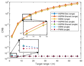
Figure 3: The CRBs of range and angle under different wavefront assumptions versus range $r$.

Fig.  3 illustrates the CRBs for range and angle estimations versus range $r$ for various wavefront assumptions. In this case, we set $r\in[1,56]$m, $\theta=\pi/3$, $K=3$ and $\Gamma_{k}=90$ for all $k\neq 0$. The SINR $\gamma=\frac{|\alpha|^{2}}{\sigma_{s}^{2}}$ is set to $0$ dB[7]. The legends “HSPM-Dist”, “HSPM-Shared”, “SWM” and “PWM” denote the CRBs for estimating range (solid lines) and angle (dashed lines) calculated as (9), (11), (12) and (13), respectively. As $r$ increases, the range CRB increases for all wavefront assumptions, whereas the angle CRB exhibits the opposite trend. Specifically, the range CRBs of HSPM-Dist and SWM nearly coincide, while HSPM-Shared exhibits a noticeable discrepancy, indicating that HSPM-Dist closely approaches the accuracy of SWM compared to HSPM-Shared. The improved performance of HSPM-Dist can be attributed to the sine function of each subarray’s unique AoA containing additional range information, as demonstrated by (4). Additionally, noticeable differences are shown among the angle CRBs under SWM, HSPM-Dist, HSPM-Shared, and PWM, indicating notable errors in the near-field region for PWM. By contrast, the angle CRBs under HSPM-Dist, HSPM-Shared, and PWM overlap closely within the interval of changing $r$. These observations indicate that the HSPM with distinct AoAs exhibits superior CRB performance compared to HSPM with shared AoA and PWM while maintaining lower complexity than SWM. Moreover, in the generic modular XL-array with non-uniformly distributed subarrays, HSPM-Shared’s assumption of identical AoAs for all subarrays becomes unreasonable. Consequently, HSPM-Dist strikes a balance between accuracy and complexity, making it the most suitable model for the generic modular XL-array architecture.

Next, we investigate the impact of different subarray layouts on the range and angle CRBs under various wavefront assumptions. According to [19], employing a centro-symmetric linear arrays can improve the near-field angle and range estimation capabilities. Therefore, we consider the centro-symmetric modular XL-array structure with subarrays arranged in a non-uniform layout symmetric about the origin. We fix the positions of subarrays at both ends of the XL-array to ensure a constant array aperture. Two subarray configurations, referred to as C1 and C2, are evaluated, with the same total number of antennas but different array apertures. For both configurations, we set $K=5$ and $M=75$. By manipulating the position parameters of the two subarrays near the origin, denoted by $\Gamma$, we can control the spacing between subarrays. Specifically, corresponding sets of inter-subarray spacings are defined as $\mathcal{I}_{1}=(100-\Gamma,\Gamma,0,\Gamma,100-\Gamma)$ and $\mathcal{I}_{2}=(150-\Gamma,\Gamma,0,\Gamma,150-\Gamma)$ for C1 and C2, respectively.

Fig. 4 illustrates the changes in range and angle CRBs as $\Gamma$ varies form $1$ to $95$. The target distance is $r=30$ m and its angle is $\theta=\pi/3$. It can be observed that the angle CRBs under both C1 and C2 configurations monotonically decrease as $\Gamma$ increases. However, the range CRBs monotonically decrease in C1 configuration , while those under C2 configuration first increase then decrease in as $\Gamma$ varies. When $\Gamma$ is set to $50$ and $75$, the subarrays in both C1 and C2 are uniformly arranged, respectively. Notably, for both C1 and C2, the range and angle CRBs of the non-uniform subarray arrangements are lower than those of the uniformly arranged subarrays when $\Gamma$ is greater than 50 and 75, respectively. This implies that the modular architecture with uniform subarray layouts is not always the most favorable configuration for near-field sensing. In order to achieve lower range and angle CRBs, subarrays of centro-symmetric modular architecture should be distributed close to the array edges.

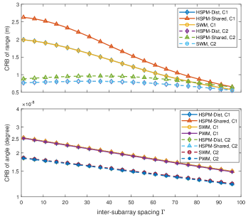
Figure 4: The CRBs of range and angle under different wavefront assumptions with different array appertures and subarray layouts.

V Conclusion

In this letter, we proposed a generic modular array architecture and derived the closed-form expressions of range and angle CRBs based on the HSPM with distinct AoAs. Numerical results were presented for validating the derived CRBs and provided the useful insights. Firstly, the HSPM with distinct AoAs demonstrates the capability to achieve lower range CRB compared to the HSPM with shared AoA, striking a good balance between modeling accuracy and complexity. This makes the HSPM with distinct AoAs more suitable for application in the generic modular array architecture. Additionally, the effectiveness of a non-uniform subarray arrangement was validated, as it could achieve lower range and angle CRB values compared to a traditional uniform subarray arrangement. This highlights the potential of the generic modular arrays in near-field sensing. For future research, subarray configurations of the generic modular array architecture should be designed considering practical installation scenarios and joint optimization of communication and sensing capabilities.

Appendix A Proof of Theorem 1

According to [20], we can obtain the CRBs for range and angle estimations, which can be given as

$$\text{CRB}_{r}\!=\!\frac{\frac{\sigma_{s}^{2}}{2}\!\left(\!\!{{\left\|{{{\mathbf{\dot{g}}}}_{\theta}}\right\|}^{2}}\!\!-\!\frac{{{\left|\mathbf{\dot{g}}_{\theta}^{H}\mathbf{g}\right|}^{2}}}{{{\left\|\mathbf{g}\right\|}^{2}}}\!\right)}{{{\left|\alpha\right|}^{2}}\det\left(\mathbf{Q}^{\prime}\right)},\ \text{CRB}_{\theta}\!=\!\frac{\frac{\sigma_{s}^{2}}{2}\!\left(\!\!{{\left\|{{{\mathbf{\dot{g}}}}_{r}}\right\|}^{2}}\!\!-\!\frac{{{\left|\mathbf{\dot{g}}_{r}^{H}\mathbf{g}\right|}^{2}}}{{{\left\|\mathbf{g}\right\|}^{2}}}\!\right)}{{{\left|\alpha\right|}^{2}}\det\left(\mathbf{Q}^{\prime}\right)},$$ (16)

where $\mathbf{g}_{\theta}=\frac{\partial\mathbf{g}}{\partial\theta}$ and $\mathbf{g}_{r}=\frac{\partial\mathbf{g}}{\partial r}$, and

$$\det\left({\mathbf{{Q}^{\prime}}}\right)=\frac{1}{{{K}^{2}}{{M}^{2}}}\left[\left(KM{{\left\|{{{\mathbf{\dot{g}}}}_{r}}\right\|}^{2}}-{{\left|\mathbf{\dot{g}}_{r}^{H}\mathbf{g}\right|}^{2}}\right)\right.\times$$ (17)

$$\left.\left(\!KM{{\left\|{{{\mathbf{\dot{g}}}}_{\theta}}\right\|}^{2}}\!\!-\!{{\left|\mathbf{\dot{g}}_{\theta}^{H}\mathbf{g}\right|}^{2}}\!\right)\!-\!\Re{{\left(\!KM\mathbf{\dot{g}}_{r}^{H}{{{\mathbf{\dot{g}}}}_{\theta}}\!-\!\mathbf{\dot{g}}_{\theta}^{H}\mathbf{g}{{\mathbf{g}}^{H}}{{{\mathbf{\dot{g}}}}_{r}}\!\right)}^{2}}\!\right].$$

According to the the rule for the derivative of the matrix multiplication with respect to the scalar, i.e.,

$$\frac{\partial\left(\mathbf{AB}\right)}{\partial x}=\frac{\partial\mathbf{A}}{\partial x}\mathbf{B}+\mathbf{A}\frac{\partial\mathbf{B}}{\partial x},$$ (18)

we have ${{\mathbf{\dot{g}}}_{u}}=\left(\text{diag}({{\dot{\bm{\nu}}}_{u}})\otimes{{\mathbf{I}}_{M}}\right)\mathbf{\tilde{a}}+\left(\text{diag}\left(\bm{\nu}\right)\otimes{{\mathbf{I}}_{M}}\right)({{\mathbf{\dot{\tilde{a}}}}_{u}}),u\in\left\{r,\theta\right\}$. By denoting ${{\dot{\bm{\nu}}}_{u}}\triangleq\frac{\partial\bm{\nu}}{\partial u}$ and ${{\mathbf{\dot{\tilde{a}}}}_{u}}\triangleq\frac{\partial\mathbf{\tilde{a}}}{\partial u}$ for all $u\in\left\{r,\theta\right\}$, we can derive the following results:

$${{{\mathbf{\dot{g}}}}_{v}}^{H}{{{\mathbf{\dot{g}}}}_{u}}$$ (19)

$$\overset{\left(a\right)}{=}\!{{{\mathbf{\tilde{a}}}}^{H}}\!\!\left(\!\text{diag}\!\left(\!{{\dot{{\bm{\nu}}}}}_{v}^{H}\!\right)\!\text{diag}\!\left(\!{{{\dot{{\bm{\nu}}}}}_{u}}\!\right)\!\otimes\!{{\mathbf{I}}_{M}}\!\right)\mathbf{\tilde{a}}\!+\!{{{\mathbf{\tilde{a}}}}^{H}}\!\left(\!\text{diag}\!\left(\!{\dot{{\bm{\nu}}}}_{v}^{H}\!\right)\!\text{diag}\!\left(\!{\bm{\nu}}\!\right)\!\otimes\!{{\mathbf{I}}_{M}}\!\right)\!{{{\mathbf{\dot{\tilde{a}}}}}_{u}}$$

$$+\mathbf{\dot{\tilde{a}}}_{v}^{H}\!\!\left(\!\text{diag}\!\left(\!{{{\bm{\nu}}}^{H}}\!\right)\!\text{diag}\!\left(\!{{{\dot{{\bm{\nu}}}}}_{u}}\!\right)\!\otimes\!{{\mathbf{I}}_{M}}\!\right)\!\mathbf{\tilde{a}}\!+\!\mathbf{\dot{\tilde{a}}}_{v}^{H}\!\!\left(\!\text{diag}\!\left({{{\bm{\nu}}}^{H}}\!\right)\!\text{diag}\!\left({\bm{\nu}}\right)\!\otimes\!{{\mathbf{I}}_{M}}\!\right)\!{{{\mathbf{\dot{\tilde{a}}}}}_{u}},$$

where $vu\in\left\{rr,r\theta,\theta\theta\right\}$, and the derivation of $(a)$ is based on the property of the Kronecker product $\left(\mathbf{A}\otimes\mathbf{B}\right)\left(\mathbf{C}\otimes\mathbf{D}\right)=\left(\mathbf{AC}\otimes\mathbf{BD}\right)$. Similarly, we can obtain that

$${{{\mathbf{\dot{g}}}}_{u}}^{H}\mathbf{g}\!=\!{\mathbf{\tilde{a}}^{H}}\!\!\left(\!\text{diag}\!\left(\!{{{\dot{\bm{\nu}}}}_{u}}^{H}\!\right)\!\text{diag}\!\left(\!\bm{\nu}\!\right)\!\otimes\!{{\mathbf{I}}_{M}}\!\right)\!\mathbf{\tilde{a}}\!+\!{{{\mathbf{\dot{\tilde{a}}}}}_{u}^{H}}\!\!\left(\!\text{diag}\!\left(\!{{\bm{\nu}}^{H}}\!\right)\!\text{diag}\!\left(\!\bm{\nu}\!\right)\!\otimes\!{{\mathbf{I}}_{M}}\!\right)\!\mathbf{\tilde{a}},$$ (20)

where $u\in\left\{r,\theta\right\}$. Furthermore, we can obtain that

$${{\mathbf{\dot{\tilde{a}}}}_{u}}=\frac{\partial{{[{{({{\mathbf{a}}_{1}})}^{T}},\ldots,{{({{\mathbf{a}}_{K}})}^{T}}]}^{T}}}{\partial u}={{\left[\frac{\partial\mathbf{a}_{1}^{T}}{\partial u},\ldots,\frac{\partial\mathbf{a}_{K}^{T}}{\partial u}\right]}^{T}},$$ (21a)

$${{\left[\frac{\partial\mathbf{a}_{k}^{T}}{\partial u}\right]}_{m}}\!\!\!=\!-j\frac{2\pi md}{\lambda}\frac{\partial\!\sin\!{{\theta}_{k}}}{\partial u}{{e}^{-j\!\frac{2\pi}{\lambda}\!md\!\sin\!{{\theta}_{k}}}},$$ (21b)

$${{\left[{{{\dot{\bm{\nu}}}}_{u}}\right]}_{k}}=-j\frac{2\pi}{\lambda}\frac{\partial{{r}_{k}}}{\partial u}{{e}^{-j\frac{2\pi}{\lambda}{{r}_{k}}}},$$ (21c)

where ${{\left[\frac{\partial\mathbf{a}_{k}^{T}}{\partial u}\right]}_{m}}$ is the $m$-th element of $\frac{\partial\mathbf{a}_{k}^{T}}{\partial u}$, and ${{\left[{{{\dot{\bm{\nu}}}}_{u}}\right]}_{k}}$ is the $k$-th element of ${{{\dot{\bm{\nu}}}}_{u}}$.

Based on (21) and (10), we can derive the expressions constituting the terms of ${{{\mathbf{\dot{g}}}}_{v}}^{H}{{{\mathbf{\dot{g}}}}_{u}}$, $vu\in\left\{rr,\theta\theta,r\theta\right\}$, which can be given by

$${{{\mathbf{\tilde{a}}}}^{H}}\left(\text{diag}\left({{{\dot{\bm{\nu}}}}_{v}}^{H}\right)\text{diag}\left({{{\dot{\bm{\nu}}}}_{u}}\right)\otimes{{\mathbf{I}}_{M}}\right)\mathbf{\tilde{a}}=M\sum\limits_{k\in\mathcal{K}}{\left[{{{\dot{\bm{\nu}}}}_{v}}\right]_{k}^{*}{{\left[{{{\dot{\bm{\nu}}}}_{u}}\right]}_{k}}}$$ (22)

$$=\!M\!{{\left(\!\frac{2\pi}{\lambda}\!\right)}^{2}}\!\!\!\sum\limits_{k\in\mathcal{K}}{\!\!\left(\!\frac{\partial{{r}_{k}}}{\partial v}\!\right)\!\!\left(\!\frac{\partial{{r}_{k}}}{\partial u}\!\right)}\!=\!M\!{{\left(\!\frac{2\pi}{\lambda}\!\right)}^{2}}\!\!\Upsilon,\Upsilon\!\!=\!\!\left\{\!\!\begin{array}[]{*{35}{l}}q,&vu=rr\\ \tilde{q},&vu=\theta\theta\\ \hat{q},&vu=r\theta\\ \end{array},\right.$$

$${{{{{\mathbf{\dot{\tilde{a}}}}}_{v}^{H}}}}\left(\text{diag}\left({{\bm{\nu}}^{H}}\right)\text{diag}\left({{{\dot{\bm{\nu}}}}_{u}}\right)\otimes{{\mathbf{I}}_{M}}\right)\mathbf{\tilde{a}}$$ (23)

$$=\!\sum\limits_{k\in\mathcal{K}}{\!\left[\bm{\nu}\right]_{k}^{*}{{\left[{{{\dot{\bm{\nu}}}}_{u}}\right]}_{k}}}\!\sum\limits_{m\in\mathcal{M}}\!{\!\left[\frac{\partial{{\mathbf{a}}_{k}}}{\partial v}\right]_{m}^{\text{*}}}\!{{\!\left[{{\mathbf{a}}_{k}}\right]}_{m}}$$

$$=\sum\limits_{k\in\mathcal{K}}{\left(-j\frac{2\pi}{\lambda}\right)\left(\frac{\partial{{r}_{k}}}{\partial u}\right)}\sum\nolimits_{m=-\frac{M-1}{2}}^{\frac{M-1}{2}}{\left(j\frac{2\pi}{\lambda}md\frac{\partial\sin{{\theta}_{k}}}{\partial v}\right)}$$

$$=\!d{{\left(\!\frac{2\pi}{\lambda}\!\right)}^{2}}\!\!\sum\limits_{k\in\mathcal{K}}\!\!{\left(\!\frac{\partial{{r}_{k}}}{\partial u}\!\right)}\!\!\left(\frac{\partial\sin{{\theta}_{k}}}{\partial v}\right)\sum\nolimits_{m=-\frac{M-1}{2}}^{\frac{M-1}{2}}{m}=0,$$

$$\mathbf{\dot{\tilde{a}}}_{v}^{H}\left(\text{diag}\left({{\bm{\nu}}^{H}}\right)\text{diag}\left(\bm{\nu}\right)\otimes{{\mathbf{I}}_{M}}\right){{{\mathbf{\dot{\tilde{a}}}}}_{u}}$$ (24)

$$={{\left(\frac{2\pi d}{\lambda}\right)}^{2}}\sum\limits_{k\in\mathcal{K}}{\left(\frac{\partial\sin{{\theta}_{k}}}{\partial v}\right)\left(\frac{\partial\sin{{\theta}_{k}}}{\partial u}\right)\sum\limits_{m=-\frac{M-1}{2}}^{\frac{M-1}{2}}{{{m}^{2}}}}$$

$$=\frac{{{M}^{3}}-M}{12}{{\left(\frac{2\pi d}{\lambda}\right)}^{2}}\sum\limits_{k\in\mathcal{K}}{\left(\frac{\partial\sin{{\theta}_{k}}}{\partial v}\right)\left(\frac{\partial\sin{{\theta}_{k}}}{\partial u}\right)}$$

$$\overset{\left(a\right)}{=}\frac{{{M}^{3}}-M}{12}{{\left(\frac{2\pi d}{\lambda}\right)}^{2}}\Xi,\Xi=\left\{\begin{array}[]{*{35}{l}}z,&vu=rr\\ \tilde{z},&vu=\theta\theta\\ \hat{z},&vu=r\theta\\ \end{array},\right.$$

where the derivation of $(a)$ is based on the fact that $\sum\nolimits_{m=-\frac{M-1}{2}}^{\frac{M-1}{2}}{{{m}^{2}}}=\frac{{{M}^{3}}-M}{12}$. Similarly, we can deduce the expressions constituting the terms of ${{{\mathbf{\dot{g}}}}_{u}}^{H}\mathbf{g}$, $u\in\left\{r,\theta\right\}$ as

$${{{\mathbf{\tilde{a}}}}^{H}}\left(\text{diag}\left({{{\dot{\bm{\nu}}}}_{u}}^{H}\right)\text{diag}\left(\bm{\nu}\right)\otimes{{\mathbf{I}}_{M}}\right)\mathbf{\tilde{a}}=j\frac{2\pi M}{\lambda}\Omega,\Omega=\!\left\{\!\begin{array}[]{*{35}{l}}p,&u=r\\ \tilde{p},&u=\theta\\ \end{array},\right.$$ (25)

$${{{{{\mathbf{\dot{\tilde{a}}}}}_{u}^{H}}}}\left(\text{diag}\left({{\bm{\nu}}^{H}}\right)\text{diag}\left(\bm{\nu}\right)\otimes{{\mathbf{I}}_{M}}\right)\mathbf{\tilde{a}}=0.$$

By substituting (22), (23), (24) and (25) into (19) and (20), we can obtain the expressions for the relevant terms as follows:

$${{{\mathbf{\dot{g}}}}_{v}}^{H}{{{\mathbf{\dot{g}}}}_{u}} ={{\left(\frac{2\pi}{\lambda}\right)}^{2}}\frac{\left({{M}^{3}}-M\right){{d}^{2}}\Xi+12M\Upsilon}{12},$$ (26)

$$\left\{\begin{array}[]{*{35}{l}}\Upsilon=q,\Xi=z,&\textit{if}\ vu=rr\\ \Upsilon=\tilde{q},\Xi=\tilde{z},&\textit{if}\ vu=\theta\theta\\ \Upsilon=\hat{q},\Xi=\hat{z},&\textit{if}\ vu=r\theta\\ \end{array},\right.$$

$${{{\mathbf{\dot{g}}}}_{u}}^{H}\mathbf{g} =j\frac{2\pi M}{\lambda}\Omega,\Omega=\left\{\begin{array}[]{*{35}{l}}p,&u=r\\ \tilde{p},&u=\theta\\ \end{array}.\right.$$

By substituting (26) into (16), we can obtain the closed-form of range/angle CRB in (9), which completes the proof.

Appendix B Proof of Corollary 1

When $\theta=0$, we have $\sin\theta_{k}=\frac{-x_{k}}{r_{k}}$, $\cos\theta_{k}=\frac{r}{r_{k}}$, and $r_{k}=\sqrt{r^{2}+x_{k}^{2}}$. Substituting these expressions into the intermediate variables in Theorem 1, we can obtain the expression of $p^{\prime}$, $q^{\prime}$, $z^{\prime}$, $\tilde{q}^{\prime}$, $\tilde{z}^{\prime}$. According to the geometric properties of centro-symmetric arrays, it can be inferred that

$$\tilde{p}\!=\!\!\sum_{k\in\mathcal{K}}\frac{-rx_{k}}{r^{2}+s_{k}^{2}}\!=\!0,\hat{q}\!=\!\!\sum_{k\in\mathcal{K}}\frac{-r^{2}x_{k}}{r^{2}+x_{k}^{2}}\!=\!0,\hat{z}\!=\!\!\sum_{k\in\mathcal{K}}\frac{r^{4}x_{k}}{r^{2}+x_{k}^{2}}\!=\!0.$$ (27)

By substituting these simplified expressions into (9) and (9), we arrive at the simplified CRB expressions in (14a) and (14b).

References

• [1] Y. Liu, Z. Wang, J. Xu, C. Ouyang, X. Mu, and R. Schober, “Near-field communications: A tutorial review,” IEEE Open J. Commun. Soc., vol. 4, pp. 1999–2049, Aug. 2023.
• [2] Z. Wang, X. Mu, and Y. Liu, “Near-field integrated sensing and communications,” IEEE Commun. Lett., vol. 27, no. 8, pp. 2048–2052, Aug. 2023.
• [3] H. Lu, Y. Zeng, C. You, Y. Han, J. Zhang, Z. Wang, Z. Dong, S. Jin, C.-X. Wang, T. Jiang, X. You, and R. Zhang, “A tutorial on near-field XL-MIMO communications towards 6G,” arXiv preprint arXiv:2310.11044, Oct. 2023.
• [4] L. Yan, Y. Chen, C. Han, and J. Yuan, “Joint inter-path and intra-path multiplexing for terahertz widely-spaced multi-subarray hybrid beamforming systems,” IEEE Trans. Commun., vol. 70, no. 2, pp. 1391–1406, Dec. 2022.
• [5] X. Li, Z. Dong, Y. Zeng, S. Jin, and R. Zhang, “Multi-user modular XL-MIMO communications: Near-field and beam focusing pattern and user grouping,” arXiv preprint arXiv:2308.11289, Aug. 2023.
• [6] X. Li, H. Lu, Y. Zeng, S. Jin, and R. Zhang, “Near-field modeling and performance analysis of modular extremely large-scale array communications,” IEEE Commun. Lett., vol. 26, no. 7, pp. 1529–1533, May 2022.
• [7] S. Yang, X. Chen, Y. Xiu, W. Lyu, Z. Zhang, and C. Yuen, “Performance bounds for near-field localization with widely-spaced multi-subarray mmWave/THz MIMO,” IEEE Trans. Wirel. Commun., pp. 1–1, 2024.
• [8] W.-C. Kao, J.-Y. Wu, S.-H. Tsai, and T.-Y. Wang, “Fast ambiguity-free subspace-based multiple AoAestimation for hybrid linear arrays,” in 2023 IEEE 34th Annual International Symposium on Personal, Indoor and Mobile Radio Communications (PIMRC), Oct. 2023, pp. 1–5.
• [9] L. Khamidullina, I. Podkurkov, and M. Haardt, “Conditional and unconditional cramér-rao bounds for near-field localization in bistatic MIMO radar systems,” IEEE Trans. Signal Process., vol. 69, pp. 3220–3234, May 2021.
• [10] Y. Zhang, H. Shan, H. Chen, D. Mi, and Z. Shi, “Perceptive mobile networks for unmanned aerial vehicle surveillance: From the perspective of cooperative sensing,” IEEE Veh. Technol. Mag., pp. 2–11, Mar. 2024.
• [11] X. Cheng, D. Duan, S. Gao, and L. Yang, “Integrated sensing and communications (ISAC) for vehicular communication networks (VCN),” IEEE Internet Things J., vol. 9, no. 23, pp. 23 441–23 451, Jul. 2022.
• [12] Y. Chen, L. Yan, and C. Han, “Hybrid spherical- and planar-wave modeling and DCNN-powered estimation of terahertz ultra-massive MIMO channels,” IEEE Trans. Commun., vol. 69, no. 10, pp. 7063–7076, July 2021.
• [13] H. Wang and Y. Zeng, “SNR scaling laws for radio sensing with extremely large-scale MIMO,” in 2022 IEEE International Conference on Communications Workshops (ICC Workshops), May 2022, pp. 121–126.
• [14] Z. Lu, Y. Han, S. Jin, M. Matthaiou, and T. Q. S. Quek, “Near-field channel reconstruction and user localization for ELAA systems,” in 2022 International Symposium on Wireless Communication Systems (ISWCS), Nov. 2022, pp. 1–6.
• [15] H. Hua, J. Xu, and Y. C. Eldar, “Near-field 3D localization via MIMO radar: Cramér-rao bound analysis and estimator design,” arXiv preprint arXiv:2308.16130, Aug. 2023.
• [16] H. Wang, Z. Xiao, and Y. Zeng, “Cramér-rao bounds for near-field sensing with extremely large-scale MIMO,” arXiv preprint arXiv:2303.05736, Mar. 2023.
• [17] H. L. V. Trees and K. L. Bell, Bayesian bounds for parameter estimation and nonlinear filtering/tracking.   Wiley-IEEE press, 2007.
• [18] Y.-D. Huang and M. Barkat, “Near-field multiple source localization by passive sensor array,” IEEE Trans. Antennas Propag., vol. 39, no. 7, pp. 968–975, Jul. 1991.
• [19] H. Gazzah and J. P. Delmas, “CRB-based design of linear antenna arrays for near-field source localization,” IEEE Trans. Antennas Propag., vol. 62, no. 4, pp. 1965–1974, Apr. 2014.
• [20] R. Boyer, “Performance bounds and angular resolution limit for the moving colocated MIMO radar,” IEEE Trans. Signal Process., vol. 59, no. 4, pp. 1539–1552, Dec. 2011.