Leveraging Domain-Unlabeled Data in Offline Reinforcement Learning across Two Domains

Abstract

In this paper, we investigate an offline reinforcement learning (RL) problem where datasets are collected from two domains. In this scenario, having datasets with domain labels facilitates efficient policy training. However, in practice, the task of assigning domain labels can be resource-intensive or infeasible at a large scale, leading to a prevalence of domain-unlabeled data. To formalize this challenge, we introduce a novel offline RL problem setting named Positive-Unlabeled Offline RL (PUORL), which incorporates domain-unlabeled data. To address PUORL, we develop an offline RL algorithm utilizing positive-unlabeled learning to predict the domain labels of domain-unlabeled data, enabling the integration of this data into policy training. Our experiments show the effectiveness of our method in accurately identifying domains and learning policies that outperform baselines in the PUORL setting, highlighting its capability to leverage domain-unlabeled data effectively.

1 Introduction

In offline reinforcement learning (RL) ²⁴, we train policies from pre-collected data without online interaction with the environment. Offline RL has been applied to real-world problems where the interaction is either cost-prohibitive or impractical, such as robotics ¹⁶, ¹⁷ and healthcare ¹³, ¹⁸. In this work, we consider offline RL problems where data is generated in two “domains” ²⁶. In such a scenario, it is crucial to identify the data’s domain and train a policy adapted to it. Previous studies often assume knowledge of domain labels and use them to train policies efficiently ²⁵, ²⁶, ³⁸. In practice, however, assigning domain labels is often costly and laborious, or sometimes infeasible. For instance, in a medical treatment scenario, the existence of a specific gene can affect the efficacy of a medication. However, as testing can be costly, few patients are tested for the gene, resulting in a small amount of labeled data and a large amount of domain-unlabeled data. In this case, the existence of the gene corresponds to a domain label. Given that the volume of data plays a pivotal role in the success of offline RL ¹⁷, ²⁸, only training on the labeled data can result in poorly performant policy. We thus need to devise a way to effectively utilize the plenty of domain-unlabeled data.

To formalize this challenge, we propose a novel offline RL problem setting called Positive-Unlabeled Offline RL (PUORL), designed for scenarios with two distinct domains where only a subset of data from one domain is labeled (Sec. 3.1). To the best of our knowledge, this is the first investigation of domain-unlabeled data in offline RL. We propose an algorithmic framework for PUORL that leverages positive-unlabeled (PU) learning ⁴, ³⁴ to train a domain identifier and utilize the identifier in the following offline RL phase (Sec. 3.2). Experiments with D4RL ⁹ with a significantly small ratio of domain-labeled data (3%) demonstrate that our method can accurately identify the domain of data and train better agents than baselines, showcasing the ability to leverage the large amount of domain-unlabeled data (Sec. 4).

2 Preliminaries

Reinforcement learning (RL).

RL ³⁵ is characterized by a Markov decision process (MDP) ³⁰, defined by 6-tuple: $(\mathcal{S},\mathcal{A},P,p_{0},r,\gamma)$. Here, $\mathcal{S}$ and $\mathcal{A}$ denote the continuous state and action spaces, respectively. $P$ defines the transition density $P:\mathcal{S}\times\mathcal{A}\times\mathcal{S}\rightarrow[0,1]$, $p_{0}$ denotes the initial state distribution $p_{0}:\mathcal{S}\rightarrow[0,1]$, $r$ specifies the reward function $r:\mathcal{S}\times\mathcal{A}\rightarrow\mathbb{R}$ and $\gamma\in[0,1)$ represents the discount factor. In RL, the primary objective is to learn a policy $\pi:\mathcal{S}\times\mathcal{A}\rightarrow[0,1]$, maximizing the expected cumulative discounted reward $\mathbb{E}_{\pi,P}\left[{\sum_{t=1}^{\infty}\gamma^{t}r(s_{t},a_{t})}\right]$, where $\mathbb{E}_{\pi,P}\left[{\cdot}\right]$ denotes the expectation over the sequence of states and actions $(s_{1},a_{1},\dots)$ generated by the policy $\pi$ and the transition density $P$.

Offline RL.

To address the limitations on direct agent-environment interactions, offline RL ²⁴ employs a fixed dataset $\mathcal{D}$ of transitions, $\mathcal{D}=\{(s_{i},a_{i},r_{i},s^{\prime}_{i})\}_{i=1}^{N}$, collected by a behavioral policy $\pi_{\beta}$. The dataset $\mathcal{D}$ is assumed to be generated independently and identically distributed ($\mathrm{i.i.d.}$) from a stationary distribution induced by the behavioral policy $\pi_{\beta}$ and $P$.

Positive-unlabeled (PU) learning.

PU learning is a method that trains a binary classifier using positive and unlabeled data ³, ³⁴. Let $X\in\mathbb{R}^{d}$ and $Y\in\{-1,+1\}$ be the random variables of the input and label in a binary classification problem. We denote the data-generating joint density over $(X,Y)$ by $p(x,y)$. Let $p_{\mathrm{p}}(x):=p(x|Y=+1)$ and $p_{\mathrm{n}}(x):=p(x|Y=-1)$ be the densities of $x$ conditioned on the positive and negative labels respectively and $p(x):=\alpha_{\mathrm{p}}p_{\mathrm{p}}(x)+\alpha_{\mathrm{n}}p_{\mathrm{n}}(x)$ be the marginal density of the unlabeled data. $\alpha_{\mathrm{p}}:=p(Y=+1)$ denotes the class prior probability (mixture proportion) for the positive label and $\alpha_{\mathrm{n}}:=p(Y=-1)=1-\alpha_{\mathrm{p}}$ for the negative label. In PU learning, we assume that we have two types of data: positively labeled data $\mathcal{X}_{\mathrm{p}}:=\{x^{\mathrm{p}}_{i}\}_{i=1}^{n_{\mathrm{p}}}\stackrel{{\scriptstyle\mathrm{i.i.d.}}}{{\sim}}p_{\mathrm{p}}(x)$ and unlabeled data $\mathcal{X}_{\mathrm{u}}:=\{x^{\mathrm{u}}_{i}\}_{i=1}^{n_{\mathrm{u}}}\stackrel{{\scriptstyle\mathrm{i.i.d.}}}{{\sim}}p(x)$. The task of PU learning is to train a binary classifier $f:X\rightarrow\{-1,+1\}$ from positive data $\mathcal{X}_{\mathrm{p}}$ and unlabeled data $\mathcal{X}_{\mathrm{u}}$. Generally, PU learning methods require information on the mixture proportion ($\alpha_{p}$) and there are a bunch of mixture proportion estimation (MPE) methods ⁷, ³², ⁸, ¹². Among the methods of PU learning, certain approaches, notably nnPU ²¹ and $(\mathrm{TED})^{\mathrm{n}}$ ¹², demonstrate particular compatibility with neural networks.

3 Method

In this section, we introduce a novel offline RL problem setting designed to leverage domain-unlabeled data with two specific objectives. Then, we propose a general algorithmic framework using PU learning for the defined problem.

3.1 Problem Formulation

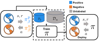
Figure 1: Diagram of Positive-Unlabeled Offline RL (PUORL). PUORL has two domains: the positive and negative. We are given two types of data: positive data, and unlabeled data—a mixture of samples from the positive and negative domains. Here, we train a domain classifier with PU learning and use the classifier in the following policy training.

We introduce positive-unlabeled offline RL (PUORL) where the dataset is generated within two distinct MDPs, with some data from one domain labeled and the rest provided as domain-unlabeled (Figure 1). Below, we proceed to define the problem setting.

Definition 1 (Positive-unlabeled offline RL (PUORL)).

In PUORL, we have two distinct MDPs, a positive MDP $\mathcal{M}_{\mathrm{p}}:=(\mathcal{S},\mathcal{A},P^{\mathrm{p}},p^{\mathrm{p}}_{0},r,\gamma)$ and a negative MDP $\mathcal{M}_{\mathrm{n}}:=(\mathcal{S},\mathcal{A},P^{\mathrm{n}},p^{\mathrm{n}}_{0},r,\gamma)$, which share the same state and action spaces and reward function. For each MDP, there exist fixed behavioral policies for each MDP $\pi^{\mathrm{p}}_{\beta}$ and $\pi^{\mathrm{n}}_{\beta}$ and they induce the stationary distributions over the state-action pair denoted as $\mu^{\mathrm{p}}(s,a)$ and $\mu^{\mathrm{n}}(s,a)$. We are given two datasets: positive data $\mathcal{D}_{\mathrm{p}}:=\{(s_{i},a_{i},r_{i},s^{\prime}_{i},+1)\}_{i=1}^{n_{\mathrm{p}}}$ and unlabeled data $\mathcal{D}_{\mathrm{u}}:=\{(s_{i},a_{i},r_{i},s^{\prime}_{i})\}_{i=1}^{n_{\mathrm{u}}}$. The positive data is sampled $\mathrm{i.i.d.}$ from $\mu^{\mathrm{p}}(s,a)$ and the domain-unlabeled data is sampled $\mathrm{i.i.d.}$ from $\mu(s,a):=\alpha_{\mathrm{p}}\mu^{\mathrm{p}}(s,a)+(1-\alpha_{\mathrm{p}})\mu^{\mathrm{n}}(s,a)$, where $\alpha_{\mathrm{p}}\in[0,1]$ is the mixture proportion. In PUORL, at the time of evaluation, we have access to the true domain labels.

Henceforth, domain-unlabeled data will be referred to as unlabeled data when it is clear from the context. The availability of true domain labels for evaluation mirrors our focus on developing methods of exploiting unlabeled data $\mathcal{D}_{\mathrm{u}}$ in the policy training phase. Although PUORL focuses on the difference in dynamics, it is straightforward to generalize the problem setting to encompass variations in the reward function as well. PUORL makes assumptions about data presentation but does not define the agents’ objectives. Among potential objectives, we consider two distinct problem settings within PUORL: single-domain and multi-domain.

Single-domain.

Here, the objective is to train an agent to achieve high performance in a domain of our interest (positive domain) despite having limited labeled data $\mathcal{D}_{\mathrm{p}}$. Meanwhile, we have a large volume of unlabeled data $\mathcal{D}_{\mathrm{u}}$, a mixture of data from the domain of our interest and a different domain (negative domain). The objective is defined as

$$\pi^{*}(a|s):=\operatornamewithlimits{argmax}_{\pi}\mathbb{E}_{\pi,P^{\mathrm{p}}}\left[{\sum_{t=1}^{\infty}\gamma^{t}r(s_{t},a_{t})}\right].$$ (1)

The most straightforward approach in this setup involves applying conventional offline RL methods on only a small amount of positive data $\mathcal{D}_{\mathrm{p}}$. However, using a small dataset increases the risk of encountering out-of-distribution state-action pairs due to the limited coverage of the dataset ²⁴. Conversely, utilizing all available data $\mathcal{D}_{\mathrm{p}}\cup\mathcal{D}_{\mathrm{u}}$ to increase the dataset size can hinder the agent’s performance due to the different dynamics ²⁶.

Multi-domain.

Contrary to the single-domain scenario, the multi-domain setting focuses on optimizing the agent’s performance in both domains. The objective is defined as

$$\forall y\in\{-1,+1\},\quad\pi^{*}(a|s,y):=\operatornamewithlimits{argmax}_{\pi}\mathbb{E}_{\pi,P_{y}}\left[{\sum_{t=1}^{\infty}\gamma^{t}r(s_{t},a_{t})}\right],$$ (2)

where $P_{+1}=P^{\mathrm{p}}$ and $P_{-1}=P^{\mathrm{n}}$. Although the problem settings are different, the fundamental challenge is analogous to that of single-domain: leveraging domain-unlabeled data while minimizing the effect of the dynamics shift.

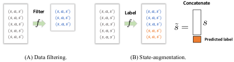
Figure 2: Diagram of our method. (A) Data filtering is a method mainly for a single domain setting, where we extract the positively predicted data from unlabeled data. (B) State augmentation is a method for a multi-domain setting, where we concatenate the state vector and predicted label.

3.2 Proposed Method

Here, we first provide a generic algorithmic framework to handle PUORL, then propose concrete algorithmic instances for the problems: single-domain and multi-domain.

General Framework.

The core concept of our approach to PUORL involves identifying the domain for each unlabeled data sample for use in offline RL. From Definition 1, we can see that PU learning, incorporating mixture proportion estimation (MPE) ¹², ³⁴, is applicable to train a classifier between two domains in PUORL. To differentiate between domains based on their dynamics, for each transition in $\mathcal{D}_{\mathrm{p}}\cup\mathcal{D}_{\mathrm{u}}$, we use $(s_{i},a_{i},s^{\prime}_{i})$ as inputs in PU learning. Building upon this formulation, we use a two-stage methodology. The first stage involves training a domain classifier through PU learning. In the second stage, we utilize the classifier in policy training with off-the-shelf offline RL algorithms. Having domain-label information removes the uncertainty in dynamics, facilitating the use of standard offline RL methods for a single MDP. This framework exhibits considerable generality, accommodating a wide range of PU learning methodologies ²¹, ¹² and offline RL approaches tailored for transition-based input ²³, ²², ¹⁰, ¹¹. Between the single-domain and multi-domain, the first step is the same and the difference is the way to use the trained classifier in the offline RL phase.

Single-domain.

In the single domain setting, to augment the positive domain data, we apply classifier $f$ to the domain-unlabeled dataset to identify instances predicted as positive, denoted by $\mathcal{D}^{f}_{\mathrm{p}}:=\{(s,a,r,s^{\prime})\in\mathcal{D}_{\mathrm{u}}:f(s,a,s^{\prime})=+1\}$, combining it with the positive data as $\tilde{\mathcal{D}}_{\mathrm{p}}:=\mathcal{D}_{\mathrm{p}}\cup\mathcal{D}^{f}_{\mathrm{p}}$. We call this process data filtering (Figure 2). Then, we train the policy using off-the-shelf offline RL methods with $\tilde{\mathcal{D}}_{\mathrm{p}}$. The details of the methodology are outlined in App. A.1. An accurate classifier is necessary for the filter approach to work well. Conversely, less accurate classifiers result in the inclusion of negative-domain data in the filtered data $\mathcal{D}^{f}_{\mathrm{p}}$, potentially leading to a performance decline due to the different dynamics.

Multi-domain.

In the multi-domain setting, we augment the state and next state for each transition by concatenating the predicted labels from the trained classifier $f$ as $s_{\mathrm{AUG}}:=(s,f(s,a,s^{\prime}))$ and $s^{\prime}_{\mathrm{AUG}}:=(s^{\prime},f(s,a,s^{\prime}))$ (Figure 1). Subsequently, an off-the-shelf offline RL algorithm is executed on the augmented data. App. A.2 explains the details of the state augmentation method. Concatenation of states and learned environment representations is commonly used in representation learning-based method in meta-RL literature ³¹, ⁵, ⁴⁰. As another way of using a classifier in multi-domain, we can conduct the data filtering twice for positive and negative domains. We experiment on the comparison in App. D.2.

4 Experiment

In this section, we first explain the general setup of our experiments and subsequently, report the results for both single-domain and multi-domain settings.

4.1 Experimental Setup

Dataset.

We utilized the widely-used D4RL benchmark ⁹ for our experiments, focusing on three control tasks: Halfcheetah, Hopper, and Walker2d. D4RL provides four different data qualities for each task: medium-expert (ME), medium-replay (MR), medium (M), and random (R). To examine the impact of dynamics shift on performance, we considered two types of dynamics shifts between positive and negative domains: body mass shift and entire body shift. In both scenarios, we maintained a positive-to-negative ratio of 3:7, resulting in a dataset of 1 million samples, with only 3% of the data labeled as positive, reflecting an unlabeled ratio of 0.97. For the body mass shift, the mass of specific body parts in the negative domain was modified, with datasets provided by ²⁶. In the entire body shift, Halfcheetah and Walker2d were paired as positive and negative domains, due to their entirely different body structures. To explore the effect of data quality on performance, we examined various combinations of data qualities, using abbreviations separated by a slash to denote pairs of positive and negative data with varying qualities, e.g., ME/ME for medium-expert quality in both domains.

Offline RL algorithms and PU learning methods.

We selected TD3+BC ¹⁰ and IQL ²² as our offline RL methods due to their widespread use and computational efficiency. The main results presented below pertain to TD3+BC. The results for IQL are reported in App. D.1. In TD3+BC, a 4-layer MLP with ReLU activation was employed for both the policy and value functions ²⁷. Layer normalization ² was applied to the value network to enhance training stability ⁴². For PU learning, $\mathrm{TED}^{\mathrm{n}}$ ¹² was chosen owing to its effectiveness with neural networks (App. B.1). To assess statistical significance, we first verified normality with the Shapiro-Wilk test. For normally distributed data, we applied Welch’s t-test; otherwise, we used the Mann-Whitney U test. For additional details about the training and evaluation, refer to App. B.

Table 1: The results of the PU classifier in the body mass shift. For each setting, we reported the average and standard deviation of the true positive rate (TPR) and accuracy (ACC) over 5 different randomly generated test datasets.

Env	Metric	ME/ME	ME/R	M/M	M/R
Hopper	TPR	$98.81\pm 0.03$	$98.08\pm 0.02$	$98.89\pm 0.03$	$95.05\pm 0.1$
	ACC	$96.30\pm 0.05$	$98.28\pm 0.03$	$96.56\pm 0.04$	$96.43\pm 0.07$
Halfcheetah	TPR	$99.13\pm 0.03$	$98.99\pm 0.02$	$98.93\pm 0.02$	$98.42\pm 0.05$
	ACC	$99.13\pm 0.02$	$99.24\pm 0.01$	$99.05\pm 0.02$	$98.89\pm 0.04$
Walker2d	TPR	$99.00\pm 0.03$	$98.43\pm 0.04$	$98.36\pm 0.02$	$98.98\pm 0.06$
	ACC	$98.64\pm 0.02$	$98.84\pm 0.03$	$98.41\pm 0.06$	$98.96\pm 0.05$

Table 2: The results in the single-domain setting with TD3+BC. We reported the average normalized score and 95% confidence interval calculated by the results from 5 different seeds. Of feasible methods (OLP, Using-All, DA, ours), we marked the best average score by blue and marked the scores having no statistical significance to the best score by bold. Separated by the double vertical line, we reported the score of the Oracle as a reference.

Body mass shift
Env	Quality	OLP	Using-All	DA	Ours	Oracle
Hopper	ME/ME	$79.3\pm 14.75$	$56.22\pm 6.58$	$69.41\pm 25.49$	$\mathbf{105.17\pm 8.61}$	$87.55\pm 18.61$
	ME/R	$79.3\pm 14.75$	$73.72\pm 36.4$	$56.95\pm 44.73$	$\mathbf{108.31\pm 6.82}$	$87.55\pm 18.61$
	M/M	$\mathbf{56.57\pm 11.38}$	$\mathbf{58.96\pm 9.61}$	$\mathbf{64.8\pm 6.44}$	$\mathbf{61.99\pm 5.32}$	$60.47\pm 6.96$
	M/R	$\mathbf{56.57\pm 11.38}$	$\mathbf{35.57\pm 26.33}$	$34.55\pm 22.48$	$\mathbf{57.94\pm 4.09}$	$60.47\pm 6.96$
Halfcheetah	ME/ME	$26.59\pm 5.27$	$82.74\pm 3.36$	$\mathbf{86.28\pm 5.24}$	$\mathbf{90.81\pm 4.45}$	$85.1\pm 10.84$
	ME/R	$26.59\pm 5.27$	$74.94\pm 12.16$	$73.63\pm 12.98$	$\mathbf{89.28\pm 7.69}$	$85.1\pm 10.84$
	M/M	$45.12\pm 0.58$	$41.21\pm 1.66$	$42.76+-1.43$	$\mathbf{48.72\pm 0.43}$	$48.58\pm 0.55$
	M/R	$\mathbf{45.12\pm 0.58}$	$\mathbf{44.82\pm 5.29}$	$\mathbf{42.76\pm 1.43}$	$\mathbf{44.92\pm 10.99}$	$48.58\pm 0.55$
Walker2d	ME/ME	$\mathbf{98.35\pm 14.19}$	$\mathbf{89.66\pm 0.85}$	$\mathbf{96.75\pm 11.89}$	$\mathbf{53.08\pm 62.69}$	$95.11\pm 42.07$
	ME/R	$\mathbf{98.35\pm 14.19}$	$\mathbf{74.19\pm 54.14}$	$\mathbf{73.33\pm 58.07}$	$\mathbf{84.42\pm 25.14}$	$95.11\pm 42.07$
	M/M	$56.96\pm 11.08$	$\mathbf{82.24\pm 0.48}$	$\mathbf{82.73\pm 0.73}$	$\mathbf{81.86\pm 5.2}$	$84.15\pm 2.68$
	M/R	$56.96\pm 11.08$	$\mathbf{59.53\pm 42.19}$	$\mathbf{77.84\pm 7.49}$	$\mathbf{69.99\pm 25.74}$	$84.15\pm 2.68$
Entire body shift
Halfcheetah	ME/ME	$26.59\pm 5.27$	$32.61\pm 10.86$	$38.92\pm 10.99$	$\mathbf{89.68\pm 6.98}$	$85.1\pm 10.84$
	ME/R	$26.59\pm 5.27$	$41.78\pm 17.19$	$41.68\pm 10.94$	$\mathbf{90.25\pm 6.78}$	$85.1\pm 10.84$

4.2 Single-Domain

Here, we conduct experiments under various settings to investigate the following four questions: (1) Can the PU learning method accurately classify the domain from PU-formatted data? (2) Can our method improve performance in the positive domain by augmenting positive data? (3) Does the magnitude of dynamics shift affect performance? (4) How does the different quality of the policy in the negative domain affect the performance?

Baselines.

To evaluate our method’s efficacy, we established four baselines for comparison: Only-Labeled-Positive (OLP), Using-All, Domain-Adaptation (DA) and Oracle. The OLP baseline, running offline RL algorithms with exclusively labeled positive data (only 3% of the entire dataset), avoided dynamics shifts’ issues at the expense of using a significantly reduced dataset size. This comparison assessed the benefit of augmenting data volume through our data filtering method. The Using-All baseline employed both positive and unlabeled data without preprocessing for offline RL, offering broader data coverage but posing the risk of performance degradation due to dynamics shifts. This comparison aimed to explore the impact of dynamics shifts and how our filtering technique can mitigate these effects. For the DA baseline, we implemented Dynamics-Aware Reward Augmentation (DARA) ²⁶, treating labeled positive data as the target domain data and unlabeled data as the source domain data. This baseline investigates the utility of leveraging unlabeled data without PU learning. Since ²⁶ also used the same control tasks in D4RL as our experiment, we utilized the same hyperparameter. For more details, refer to App. C.1. Lastly, the Oracle baseline, training policy with positively labeled data and all positive data within the unlabeled data, provides the ideal performance our method strives to achieve.

Can the PU learning method accurately classify the domain from the PU-formatted data?

As observed in Table 1, the true positive rates surpassed 95% across all configurations, suggesting the accurate data filtering in our method. More results on the classifier performance are in App. D.3.

Can our method improve performance in the positive domain by augmenting positive data?

In the single domain setting, our method outperformed the OLP, Using-All, and DA baselines in more than half of the configurations (8 out of 14), achieving statistically significant improvements in certain Hopper and Halfcheetah settings, as detailed in Table 2. In scenarios where our method did not lead, it still performed competitively, showing no significant statistical inferiority to the top-performing baselines. Across all configurations, our method’s performance was at least on par with the Oracle baseline, benefiting from access to accurate labels. The superiority of our method over the OLP and Using-All baselines illustrates its efficacy in augmenting data volume and preventing performance degradation from dynamics shifts via precise data filtering. Achieving higher performance than the DA baseline, attempting to leverage domain-unlabeled data, highlights the significant advantages of employing PU learning in PUORL.

Does the magnitude of dynamics shift affect performance?

The performances of the Using-All and DA baselines, as depicted in Table 2, saw significant deterioration when the unlabeled data included negative samples exhibiting large dynamics shifts, specifically in the Halfcheetah ME/ME and ME/R settings. Here, the entire body shift resulted in a substantial decrease in performance in comparison with a body mass shift. Conversely, our method exhibited stable performance across both types of dynamics shifts, highlighting its resilience against domain dynamics variations.

How does the different quality of negative domain data affect the performance?

As Table 2 illustrates, the Using-All and DA baselines, which utilized the unlabeled data in their training processes, experienced significant declines in performance when trained on lower quality negative data. Conversely, the performance of our method remained stable across various qualities of negative data, highlighting its resilience to variations in the quality of negative data.

Table 3: The results in the multi-domain setting with TD3+BC. We marked the best average normalized score by blue and marked the scores having no statistical significance to the best score by bold. We abbreviated positive, negative, and state augmentation as pos, neg, and s-aug.

Body mass shift
Env	Quality	Unsupervised	Ours (s-aug)	Oracle (s-aug)
Hopper	ME/ME (pos)	$0.74\pm 0.24$	$\mathbf{105.89\pm 8.17}$	$87.14\pm 16.25$
	ME/ME (neg)	$0.74\pm 0.24$	$\mathbf{47.52\pm 5.7}$	$\mathbf{41.7\pm 8.53}$
	M/M (pos)	$1.3\pm 0.43$	$\mathbf{57.83\pm 5.59}$	$\mathbf{56.67\pm 8.13}$
	M/M (neg)	$1.29\pm 0.43$	$\mathbf{29.94\pm 11.95}$	$\mathbf{31.6\pm 12.83}$
Halfcheetah	ME/ME (pos)	$0.03\pm 1.04$	$75.97\pm 9.15$	$\mathbf{87.34\pm 2.56}$
	ME/ME (neg)	$0.01\pm 1.14$	$\mathbf{66.08\pm 2.36}$	$\mathbf{66.36\pm 2.78}$
	M/M (pos)	$6.11\pm 13.12$	$\mathbf{47.5\pm 0.25}$	$\mathbf{47.34\pm 0.49}$
	M/M (neg)	$5.82\pm 13.14$	$\mathbf{40.49\pm 0.31}$	$\mathbf{40.56\pm 0.35}$
Walker2d	ME/ME (pos)	$-0.21\pm 0.3$	$96.37\pm 26.62$	$\mathbf{110.64\pm 0.68}$
	ME/ME (neg)	$-0.21\pm 0.3$	$-0.72\pm 0.25$	$\mathbf{89.41\pm 1.08}$
	M/M (pos)	$-0.2\pm 0.16$	$\mathbf{74.17\pm 10.49}$	$\mathbf{69.81\pm 30.89}$
	M/M (neg)	$-0.2\pm 0.16$	$0.27\pm 2.49$	$\mathbf{82.95\pm 1.17}$
Entire body shift
Halfcheetah	ME/ME (pos)	$-1.39\pm 1.18$	$60.18\pm 11.63$	$\mathbf{72.76\pm 9.3}$
	ME/ME (neg)	$-0.4\pm 0.03$	$\mathbf{64.77\pm 21.17}$	$\mathbf{53.41\pm 20.67}$

4.3 Multi-Domain

Here, we explain experiments evaluating our method in the multi-domain setting.

Baselines.

To examine the impact of domain representation variations under different domain information assumptions on performance, we compared our method with two baselines. The first is Oracle, with access to true domain labels, concatenating the states with the true domain labels in the dataset and offline RL algorithms with that. The second is Unsupervised, for scenarios with hidden domain labels, employing state-action-next-state $(s,a,s^{\prime})$ pairs for context encoding. Following existing methods ⁵, ¹, we utilized VAE (Variational Auto-Encoder) ¹⁹ to learn domain representations. For more detailed methodology, refer to App. C.2. Since we assume the accessibility to the true domain labels in evaluation, we provided state vectors concatenated with true domain labels for both our method and the Oracle baseline during the evaluation phase, while the Unsupervised baseline augmented the state by concatenating the state vector with the learned representation.

Results.

Table 3 shows that our method outperformed the Unsupervised baseline in 12 out of 14 scenarios, demonstrating its clear superiority over unsupervised context-encoding methods. A Hypothesis is that the Unsupervised baseline’s performance was hampered by the lack of ordering information, particularly regarding the initial step and short history length in the dataset. For a more detailed explanation of the hypothesis, refer to App. C.2. Additionally, our method achieved results that were comparable to the Oracle in 9 scenarios, with better average or no statistically significant difference. Overall, our results highlight the benefits of using representations from PU learning over entirely unsupervised methods, nearly matching the performance achievable with true domain labels. We further explored the comparison between the state augmentation method and the data filtering method in App. D.2.

5 Related Work

RL with multiple MDPs.

Contextual MDPs (CMDPs) formalize the RL problem with multiple environments as MDPs controlled by a variable known as a “context” ¹⁴. Different types of contexts are used to define different types of problems ²⁰. We focus on the case where the context is a binary task ID that determines the dynamics. Thanks to its generality, the CMDP can encapsulate a wide range of RL problems, such as multi-task RL ⁴³, ²⁵, ³³ and meta-RL ⁴⁴, ⁵. Depending on the observability of the context, the solution to the RL problem within CMDPs differs. If the context is observable, we can utilize the information in policy training. For example, acquiring a representation of the environment using self-supervised learning ³³, ¹⁵, ¹, ²⁵ is common in addressing this objective. In offline RL, MBML (Multi-task Batch RL with Metric Learning) employed metric learning to acquire a robust representation of discrete contexts in an offline setting ²⁵. Unlike these approaches, our method considers settings where only a subset of the data has observable contexts.

CMDPs with unobservable contexts are also known as Hidden-Parameter (HiP)-MDPs ⁶, ²⁹. In HiP-MDPs, previous works typically focused on training an inference model for the context from histories of multiple time steps ³¹, ⁴⁴, ⁴⁰, ⁵. Since we consider transition-based datasets without trajectory information, such methods are not applicable in our setting.

Unlabeled data in RL.

In previous work, “unlabeled data” refers to two settings: reward-unlabeled data and data with the quality of the behavioral policy unknown. In the first case, the unlabeled data consist of transitions without rewards ³⁷, ⁴⁵, ⁴¹. Several studies have attempted to learn the reward function from reward-unlabeled data using the PU learning technique and then utilize this learned reward function in subsequent RL routines ³⁷, ⁴⁵. In the offline multi-task RL literature, ⁴¹ explored using reward-unlabeled data in a conservative way, i.e., setting the reward of the unlabeled transitions to zero. In our study, the label corresponds to a specific domain while they regard the reward as a label. In the second case, the unlabeled data is a mixture of transitions from policies of unknown quality. In offline RL, previous works attempted to extract high-quality data from unlabeled data using PU learning ³⁶, ³⁹. In our setting, labels correspond to specific domains, not the quality of the behavioral policy.

6 Limitations and Future Work

PUORL considers two domains, and we exploit the assumption to leverage domain-unlabeled data through PU learning. The inability to address data from more than two domains is the main limitation, and overcoming this limitation is a promising direction. Indeed, PU learning is a subset of weakly supervised learning (WSL) ³⁴, a paradigm where models are trained under less informative supervision than traditional fully supervised approaches. By extending the problem setting to other WSL problems, we expect to broaden the applicability of offline RL in more practical scenarios, including a setting where data is collected in more than two domains.

Our approach primarily focuses on identifying the domain and trains a policy exclusively with the data from the domain of our interest. Thus, developing an efficient method to share data from another domain to improve performance in the domain of interest is a potential future direction.

7 Conclusion

In this study, we proposed a novel offline RL problem setting, termed positive-unlabeled offline RL (PUORL), which incorporates domain-unlabeled data. In PUORL, we explored two distinct problem settings: single-domain and multi-domain. Subsequently, we introduced a generic algorithmic framework for PUORL, utilizing PU learning and provided concrete instances for both single-domain and multi-domain settings. Our experimental validation, conducted on the D4RL benchmark against diverse baselines, demonstrated that our approach with PU learning trains policies that achieve strong performance by leveraging significant amounts of domain-unlabeled data in both settings.

Appendix A Detailed Explanation of Our Algorithms

In this section, we provide a detailed explanation of our method, covering both single-domain and multi-domain settings. The explanation primarily utilizes pseudo-code to illustrate our method.

A.1 Single-Domain

Here, we provide a pseudo code for the data filtering method in Algo. 1.

Algorithm 1 Data filtering for the positive domain

1:Initialize classifier parameters $\psi$ of classifier $f$

2:Initialize policy parameters $\theta$ and value function parameters $\phi$

3:Initialize experience replay buffer $\mathcal{D}_{\mathrm{p}}$ and $\mathcal{D}_{\mathrm{u}}$

4:Specify epochs $K_{\mathrm{PU}}$, $K_{\mathrm{RL}}$

5:for iteration $k\in[0,\dots,K_{\mathrm{PU}}]$ do $\triangleright$ PU learning routine

6:     Update $\psi$ on $\mathcal{D}_{\mathrm{p}}$ and $\mathcal{D}_{\mathrm{u}}$ by PU learning method

7:end for

8:$\tilde{\mathcal{D}}_{\mathrm{p}}\leftarrow\mathcal{D}_{\mathrm{p}}\cup\{(s,a,r,s^{\prime})\in\mathcal{D}_{\mathrm{u}}:f_{\psi}(s,a,s^{\prime})=+1\}$ $\triangleright$ Augment positive data

9:for iteration $k\in[0,\dots,K_{\mathrm{RL}}]$ do $\triangleright$ Offline RL routine

10:     Update $\theta$ and $\phi$ on $\tilde{\mathcal{D}}_{\mathrm{p}}$ by Offline RL method

11:end for

12:Output $\theta$ and $\phi$

A.2 Multi-Domain

Here, we offer a detailed explanation of the state augmentation method for a multi-domain scenario, as outlined in Algo. 3. In the evaluation phase, given that PUORL assumes access to the true label, we augment the state with the true label and feed it to the trained agent.

Algorithm 2 State augmentation

1:Trained classifier $f$ and offline RL dataset $\mathcal{D}$

2:Initialize augment data $\mathcal{D}_{\mathrm{AUG}}$.

3:for iteration $(s,a,r,s^{\prime})\in\mathcal{D}$ do

4:     Concatenate state $s$ and next state $s^{\prime}$ by prediction label into $s_{\mathrm{AUG}}$ and $s^{\prime}_{\mathrm{AUG}}$

5:     $\mathcal{D}_{\mathrm{AUG}}\leftarrow\mathcal{D}_{\mathrm{AUG}}\cup(s_{\mathrm{AUG}},a,s^{\prime}_{\mathrm{AUG}},r)$

6:end for

Algorithm 3 Multi-domain state augmentation

1:Initialize classifier parameters $\psi$ of classifier $f$

2:Initialize policy parameters $\theta$ and value function parameters $\phi$

3:Initialize experience replay buffer $\mathcal{D}_{\mathrm{p}}$ and $\mathcal{D}_{\mathrm{u}}$

4:Specify epochs $K_{\mathrm{PU}}$, $K_{\mathrm{RL}}$

5:for iteration $k\in[0,\dots,K_{\mathrm{PU}}]$ do $\triangleright$ PU learning routine

6:     Update $\psi$ on $\mathcal{D}_{\mathrm{p}}$ and $\mathcal{D}_{\mathrm{u}}$ by PU learning method

7:end for

8:Generate $\tilde{\mathcal{D}}_{\mathrm{AUG}}$ $\triangleright$ State augmentation

9:for iteration $k\in[0,\dots,K_{\mathrm{RL}}]$ do $\triangleright$ Offline RL routine

10:     Update $\theta$ and $\phi$ on $\tilde{\mathcal{D}}_{\mathrm{AUG}}$ by Offline RL method

11:end for

TD3+BC
Critic Learning Rate	$3\times 10^{-4}$
Actor Learning Rate	$3\times 10^{-4}$
Discount Factor	0.99
Target Update Rate	$5\times 10^{-3}$
Policy Noise	0.2
Policy Noise Clipping	(-0.5, 0.5)
Policy Update Frequency	Variable
TD3+BC Hyperparameter $\alpha$	2.5
Actor Hidden Dims	(256, 256)
Critic Hidden Dims	(256, 256)
IQL
Critic Learning Rate	$3\times 10^{-4}$
Actor Learning Rate	$3\times 10^{-4}$
Discount Factor	0.99
Expectile	0.7
Temperature	3.0
Target Update Rate	$5\times 10^{-3}$
Actor Hidden Dims	(256, 256)
Critic Hidden Dims	(256, 256)

Table 4: Hyperparameters for TD3+BC and IQL.

Appendix B Details of Experimental Setup

B.1 PU Learning

Explanation of $\mathrm{TED}^{\mathrm{n}}$ ¹².

Here, we briefly explain the $\mathrm{TED}^{\mathrm{n}}$ ¹² we used in our experiments. $\mathrm{TED}^{\mathrm{n}}$ consists of two subroutines for the mixture proportion estimation, Best Bin Estimation (BBE), and for PU learning, Conditional Value Ignoring Risk (CVIR). They iterate these subroutines. Given the estimated mixture proportion $\hat{\alpha}$ by BBE, CVIR first discards $\hat{\alpha}$ samples from unlabeled data based on the output probability of being positive from the current classifier $f$. The discarded samples are seemingly positive data. Then, the classifier is trained using the labeled positive data and the remaining unlabeled data. On the other hand, in BBE, we estimate the mixture proportion using the output of the classifier $f$ with the samples in the validation dataset as inputs.

Training and evaluation.

The PU learning method $\mathrm{TED}^{\mathrm{n}}$ involved two phases: warm-up and main training. We assigned 3 epochs for the warm-up step and 20 epochs for the main training step. For the classifier’s network architecture, we utilized a 3-layer MLP with ReLU. In our method, the trained classifier was then frozen and shared across different random seeds of offline RL training with identical data generation configurations, such as the positive-to-negative and unlabeled ratios. To ensure the classifier’s accuracy and stability amidst random variations in dataset generation, we generated five random test datasets for each configuration. We then evaluated the frozen classifier’s accuracy with these datasets and reported the average and standard deviation. We reported the average and standard deviation of the true positive rate and accuracy.

B.2 Offline RL

For offline RL, we learned a policy with 1 million update steps. For both TD3+BC and IQL, we used the same hyperparameters for all baselines and settings (Table 4). We evaluated the offline RL agent using the normalized score provided by D4RL ⁹. To evaluate the algorithmic stability of the offline RL routine, we conducted training with 5 different random seeds. For each seed, we calculated the average normalized score over 10 episodes. We reported the overall mean and 95% confidence interval from these averaged scores. We first tested whether both data followed the normal distribution by the Shapiro-Wilk test. If both followed normal, we used Welch’s t test, if not, we used the Mann–Whitney U test. We reported the statistical significance with a $p$-value of $0.05$.

Algorithm 4 DARA

1:Target offline data $\mathcal{D}_{\mathrm{t}}$ and source offline data $\mathcal{D}_{\mathrm{s}}$ and $\eta$.

2:Learn classifier $q_{\mathrm{sas}}:\mathcal{S}\times\mathcal{A}\times\mathcal{S}\rightarrow[0,1]$ and $q_{\mathrm{sa}}:\mathcal{S}\times\mathcal{A}\rightarrow[0,1]$ from $\mathcal{D}_{\mathrm{t}}$ and $\mathcal{D}_{\mathrm{s}}$.

3:For all $(s,a,r,s^{\prime})$ in $\mathcal{D}_{\mathrm{s}}$:

$$\Delta r(s,a,s^{\prime})=\log\frac{q_{\mathrm{sas}}(\mathrm{source}|s,a,s^{\prime})}{q_{\mathrm{sas}}(\mathrm{target}|s,a,s^{\prime})}+\log\frac{q_{\mathrm{sa}}(\mathrm{source}|s,a)}{q_{\mathrm{sa}}(\mathrm{target}|s,a)}$$ (3)

$$r\leftarrow r-\eta\Delta r$$ (4)

4:Learn policy with $\mathcal{D}_{\mathrm{t}}\cup\mathcal{D}_{\mathrm{s}}$.

Appendix C Baselines

Here, we provide a detailed explanation of the Domain-Adaptation baseline and Unsupervised baseline.

C.1 Domain-Adaptation baseline

Here, we explain the Domain-Adaptation (DA) baseline used in Section 4.2. For domain adaptation in offline RL, we utilized the Dynamics-Aware Reward Augmentation (DARA) ²⁶. In domain adaptation in offline RL, we focus on the performance in a target domain $\mathcal{M}_{\mathrm{t}}$ with a limited amount of target domain data $\mathcal{D}_{\mathrm{t}}$. To address this scarcity, domain adaptation uses data $\mathcal{D}_{s}$ from the source domain $\mathcal{M}_{\mathrm{s}}$. DARA modifies the source domain data’s reward using a trained domain classifier and then utilizes this data with the modified reward for offline RL. Lacking full domain labels in PUORL, we treated the positive data $\mathcal{D}_{\mathrm{p}}$ as target domain data, and the domain-unlabeled data $\mathcal{D}_{\mathrm{u}}$ as source domain data, training the classifier with 20 epochs accordingly. We set $\eta=0.1$ following original paper ²⁶.

Algorithm 5 Training of context encoder model

1:Offline RL dataset $\mathcal{D}$ (batched).

2:Initialize encoder parameter $\psi_{\mathrm{enc}}$ and decoder parameter $\psi_{\mathrm{dec}}$

3:for iteration $(s,a,r,s^{\prime})\in\mathcal{D}$ do

4:     Set context as $c=(s,a,s^{\prime})$

5:     Obtain mean $\mu$ and the variance $\sigma$ of the latent distribution from the encoder $f_{\psi_{\mathrm{enc}}}$ by feeding $c$

6:     Sample a latent vector $z\sim\mathcal{N}(\mu,\mathrm{diag}(\sigma))$

7:     Predict $s^{\prime}$ from $s,a$ and $z$ as $\tilde{s}^{\prime}=g_{\psi_{\mathrm{dec}}}(s,a,z)$

8:     Calculate loss VAE loss and update $\psi_{\mathrm{enc}}$ and $\psi_{\mathrm{dec}}$

9:end for

10:Output $f_{\psi_{\mathrm{enc}}}$

Algorithm 6 Training of TD3+BC with VAE

1:Initialize TD3+BC policy parameter $\theta$ and value function $\phi$

2:Initialize augmented dataset $\mathcal{D}_{\mathrm{AUG}}$

3:Train VAE and obtain encoder $f_{\psi_{\mathrm{enc}}}$ using Algo. 5.

4:for iteration $(s,a,r,s^{\prime})\in\mathcal{D}$ do

5:     Concatenate state and next state with the mean of context embedding $\mu$ from the encoder $f_{\psi_{\mathrm{enc}}}(c)$, where $c=(s,a,s^{\prime})$

$$\bar{s}_{\mathrm{AUG}}:=(s,\mu)$$

$$\bar{s}^{\prime}_{\mathrm{AUG}}:=(s^{\prime},\mu)$$

6:     $\mathcal{D}_{\mathrm{AUG}}\leftarrow\mathcal{D}_{\mathrm{AUG}}\cup\{(\bar{s}_{\mathrm{AUG}},a,r,\bar{s}^{\prime}_{\mathrm{AUG}})\}$

7:end for

8:Update $\theta$ and $\phi$ using TD3+BC.

9:Output $\theta$ and $\phi$.

Algorithm 7 Evaluation step of trained policy with encoder

1:MDP $(\mathcal{S},\mathcal{A},P,p_{0},r,\gamma)$ in which we evaluate a policy.

2:Trained policy $\pi$ and context encoder $f$.

3:Obtain initial state $s_{0}$ from initial distribution $p_{0}$.

4:Initialize $t=0$

5:while Not terminated do

6:     if t=0 then

7:         $\mu_{t}=\mathbf{0}$ $\triangleright$ The prior mean of latent vector

8:     else

9:         $\mu_{t}=f(a_{t-1},s_{t-1},s_{t})$ $\triangleright$ Obtain the mean latent vector from context encoder

10:     end if

11:     $s^{\mathrm{AUG}}_{t}=(s_{t},\mu_{t})$ $\triangleright$ Concatenate the latent vector and the current state

12:     Policy selects action $a=\pi(s^{\mathrm{AUG}}_{t})$.

13:     Transit to next state $s_{t+1}$ following $P(\cdot|s,a)$ and receive reward $r_{t}=r(s_{t},a_{t})$

14:     $t\leftarrow t+1$

15:end while

C.2 Unsupervised baseline

Here, we provide a detailed explanation of the Unsupervised baseline for the multi-domain used in Section 4.3. The overall training process follows the BOReL ⁵, an offline meta-RL algorithm that employs VAE ¹⁹ to learn task representations from trajectory inputs. Since the longest sequence of state actions from the same episode in our setting is a transition, $(s,a,s^{\prime})$, we train VAE using the transitions as inputs. The encoder outputs the mean $\mu\in\mathbb{R}^{d}$ and variance $\sigma\in\mathbb{R}^{d}$ of the normal distribution $\mathcal{N}(\mu,\mathrm{diag}(\sigma))$, where the latent representation of the domain sampled from $z\sim\mathcal{N}(\mu,\mathrm{diag}(\sigma))$ ($\mathrm{diag}(\sigma)$ denotes the diagonal matrix with its diagonal elements $\sigma$). We set $d$ as 16 in this experiment.

In BOReL, the decoder is divided into a reward decoder and a next-state decoder. However, focusing on the dynamics shift, we exclusively train the next state decoder $g:\mathcal{S}\times\mathcal{A}\times\mathbb{R}^{d}\rightarrow\mathcal{S}$. Both the encoder and the next state decoder are represented by 3-layer MLPs with ReLU. The VAE objective is the summation of reconstruction loss of the next state decoder and Kullback–Leibler (KL) divergence between the latent distribution and prior, standard normal distribution over $\mathbb{R}^{d}$. We offered the detailed procedure in Algo. 5. For the offline RL training combined with VAE training, please refer to Algo. 6. As for the evaluation, in each time step $t>0$, the context encoder predicts the mean of the latent vector $\mu_{t}$ from the current context $(a_{t-1},s_{t-1},s_{t})$ and policy outputs action based on the augmented state $(s_{t},\mu_{t})$. For the initial step $t=0$, since we do not have the context, we substitute the mean of the latent distribution for that of prior $\mathbf{0}\in\mathbb{R}^{d}$. For more details, please refer to Algo. 7.

Hypotheses on the difficulty in PUORL.

Here, we explain some hypotheses on why the Unsupervised baseline performed poorly in PUORL: the lack of ordering information and the short history length, both stemming from the fact that our dataset is transition-based. At evaluation, we augment the initial state with the prior mean (a 0 vector). However, since we lack information about which transition originates from the initial state, we cannot effectively train a policy for states augmented by the prior mean, potentially causing extremely poor performance in the initial state. Secondly, the longest sequence in our dataset is a transition $(s,a,s^{\prime},r)$, whereas, in BOReL, the history length for the VAE input exceeds 100 for control tasks in D4RL. We speculate that the short history length may result in inadequate domain representation, leading to low performance.

Table 5: The results with IQL in the single domain setting. We reported the average normalized score and 95% confidence interval calculated by the results from 5 different seeds. We marked the best average score by blue and marked the scores having no statistical significance to the best score by bold.

Body mass shift
Env	Quality	ours	Oracle
Hopper	ME/ME	$\mathbf{49.69\pm 11.61}$	$\mathbf{46.15\pm 13.59}$
	ME/R	$12.23\pm 9.01$	$\mathbf{46.15\pm 13.59}$
	M/M	$\mathbf{43.33\pm 22.6}$	$\mathbf{48.68\pm 6.35}$
	M/R	$14.37\pm 13.84$	$\mathbf{48.68\pm 6.35}$
Halfcheetah	ME/ME	$\mathbf{59.17\pm 8.01}$	$\mathbf{62.54\pm 11.85}$
	ME/R	$\mathbf{63.29\pm 4.8}3$	$\mathbf{62.54\pm 11.85}$
	M/M	$41.16\pm 2.02$	$\mathbf{42.35\pm 0.48}$
	M/R	$\mathbf{42.11\pm 1.13}$	$\mathbf{42.35\pm 0.48}$
Walker2d	ME/ME	$48.55\pm 30.78$	$\mathbf{104.13\pm 7.52}$
	ME/R	$37.21\pm 26.87$	$\mathbf{104.13\pm 7.52}$
	M/M	$\mathbf{48.82\pm 36.3}$	$\mathbf{68.93\pm 3.04}$
	M/R	$40.77\pm 36.38$	$\mathbf{68.93\pm 3.04}$
Entire body shift
Halfcheetah	ME/ME	$\mathbf{62.92\pm 9.66}$	$\mathbf{61.12\pm 11.69}$
	ME/R	$\mathbf{59.15\pm 6.91}$	$\mathbf{62.97\pm 21.7}$

Table 6: The results with IQL in multi-domain setting. We marked the best average normalized score by blue and marked the scores having no statistical significance to the best score by bold. In the table, we abbreviated positive, negative, and state augmentation as pos, neg, and s-aug.

Body mass shift
Env	Quality	Ours (s-aug)	Oracle (s-aug)
Hopper	ME/ME (pos)	$\mathbf{50.82\pm 15.08}$	$\mathbf{61.87\pm 14.7}$
	ME/ME (neg)	$15.83\pm 4.89$	$\mathbf{33.04\pm 9.01}$
	M/M (pos)	$\mathbf{50.65\pm 3.74}$	$\mathbf{51.13\pm 4.76}$
	M/M (neg)	$\mathbf{16.77\pm 1.54}$	$\mathbf{17.95\pm 4.5}$
Halfcheetah	ME/ME (pos)	$\mathbf{44.36\pm 6.86}$	$\mathbf{47.9\pm 2.95}$
	ME/ME (neg)	$\mathbf{37.16\pm 0.76}$	$\mathbf{37.41\pm 0.3}$
	M/M (pos)	$\mathbf{41.6\pm 1.67}$	$\mathbf{41.81\pm 1.92}$
	M/M (neg)	$\mathbf{37.34\pm 0.29}$	$\mathbf{37.22\pm 0.21}$
Walker2d	ME/ME (pos)	$74.52\pm 5.52$	$\mathbf{107.29\pm 1.68}$
	ME/ME (neg)	$\mathbf{19.41\pm 47.74}$	$\mathbf{86.76\pm 0.95}$
	M/M (pos)	$\mathbf{71.75\pm 5.07}$	$\mathrm{70.18\pm 6.03}$
	M/M (neg)	$10.84\pm 25.53$	$\mathbf{75.79\pm 7.33}$
Entire body shift
Halfcheetah	ME/ME (pos)	$\mathbf{43.41\pm 4.56}$	$\mathbf{43.51\pm 6.54}$
	ME/ME (neg)	$\mathbf{103.95\pm 5.03}$	$\mathbf{97.78\pm 17.78}$

Appendix D Supplemental result

In this section, we present the supplementary results and discussion to provide additional insights into the main findings.

D.1 Results with IQL

Here, we provide the experimental results with IQL ²². We used our own implementation of IQL in the experiments. For both the single-domain and multi-domain settings, we compared our method with the Oracle baseline. For single-domain settings, Table 5 demonstrates that in 8 out of 14 cases for both single-domain, our method showed no statistical significance when compared to the Oracle baseline. Furthermore, Table 6 shows that in 11 out of 14 settings in multi-domain, our method was not statistically inferior to the oracle.

D.2 State Augmentation V.S. Data Filtering in Multi-Domain

Table 7: The comparison of the state augmentation method and data filtering method for ours and the Oracle baseline in the multi-domain setting. The offline RL algorithm was TD3+BC. We reported the average normalized score and 95% confidence interval calculated by the results from 5 different seeds. For both our method and the Oracle baseline, if one of the two versions was superior to the other with statistical significance, we marked the better one with blue.

Body mass shift
Env	Quality	ours (s-aug)	ours (filter)	oracle (s-aug)	oracle (filter)
Hopper	ME/ME (pos)	$105.89\pm 8.17$	$105.17\pm 8.61$	$87.14\pm 16.25$	$87.55\pm 18.61$
	ME/ME (neg)	$47.52\pm 5.7$	$45.89\pm 6.84$	$41.7\pm 8.53$	$40.74\pm 8.48$
	M/M (pos)	$57.83\pm 5.59$	$61.99\pm 5.32$	$56.67\pm 8.13$	$60.47\pm 6.96$
	M/M (neg)	$29.94\pm 11.95$	$29.35\pm 13.32$	$31.76\pm 14.28$	$31.76\pm 14.28$
Halfcheetah	ME/ME (pos)	$75.97\pm 9.15$	$\mathbf{90.81\pm 4.45}$	$87.34\pm 2.56$	$85.1\pm 10.84$
	ME/ME (neg)	$66.08\pm 2.36$	$68.04\pm 1.34$	$66.36\pm 2.78$	$66.02\pm 2.19$
	M/M (pos)	$47.5\pm 0.25$	$\mathbf{48.72\pm 0.43}$	$47.34\pm 0.49$	$\mathbf{48.58\pm 0.55}$
	M/M (neg)	$40.49\pm 0.31$	$\mathbf{41.13\pm 0.34}$	$40.56\pm 0.35$	$\mathbf{41.18\pm 0.11}$
Walker2d	ME/ME (pos)	$96.37\pm 26.62$	$53.08\pm 62.69$	$110.64\pm 0.68$	$95.11\pm 42.07$
	ME/ME (neg)	$-0.72\pm 0.25$	$-0.49\pm 0.41$	$89.41\pm 1.08$	$89.26\pm 0.87$
	M/M (pos)	$74.17\pm 10.49$	$\mathbf{81.86\pm 5.2}$	$69.81\pm 30.89$	$\mathbf{84.15}\pm 2.68$
	M/M (neg)	$0.27\pm 2.49$	$-0.61\pm 0.15$	$82.95\pm 1.17$	$82.16\pm 1.18$
Entire body shift
Halfcheetah	ME/ME (pos)	$60.18\pm 11.63$	$\mathbf{89.68\pm 6.98}$	$72.76\pm 9.3$	$\mathbf{85.1\pm 10.84}$
	ME/ME (neg)	$64.77\pm 21.17$	$\mathbf{109.5\pm 0.89}$	$53.41\pm 20.67$	$\mathbf{89.26\pm 0.87}$

Here, we compare state augmentation and data filtering for both our method and the Oracle baseline. As shown in Table 7. For body mass shifts, no significant performance difference was observed in 17 of 24 settings. Specifically, our method showed no statistical advantage in 8 of 12 settings, and the Oracle in 9 of 12 settings. Conversely, in the entire body shifts, data filtering proved superior with statistical significance in all settings.

Table 8: The average and standard deviation of true positive rate and accuracy of the PU classifier in the entire body shift. The report protocol is the same as table 1.

	True Positive Rate (%)		Accuracy (%)
Env	ME/ME	ME/R	ME/ME	ME/R
Halfcheetah	$99.65\pm 0.02$	$99.47\pm 0.04$	$99.76\pm 0.01$	$99.64\pm 0.03$

D.3 Classifier Performance

Here, we review the performance of the classifier under the entire body shift. First, we re-mention the dataset. The ratio of positive and negative data is 3:7, and the total amount of the samples is 1 million. The unlabeled ratio is 97%, making only 3% of positively labeled data. As Table 8 illustrates, the trained classifier achieved higher than 99% true positive rate and accuracy, demonstrating the efficacy of PU learning under entire body shift.

References

- Achiam et al. [2018] Joshua Achiam, Harrison Edwards, Dario Amodei, and P. Abbeel. Variational Option Discovery Algorithms. arXiv preprint arXiv:1807.10299, 2018.
- Ba et al. [2016] Jimmy Lei Ba, Jamie Ryan Kiros, and Geoffrey E Hinton. Layer normalization. arXiv preprint arXiv:1607.06450, 2016.
- Bekker & Davis [2018] Jessa Bekker and Jesse Davis. Estimating the class prior in positive and unlabeled data through decision tree induction. In Proceedings of the Thirty-Second AAAI Conference on Artificial Intelligence and Thirtieth Innovative Applications of Artificial Intelligence Conference and Eighth AAAI Symposium on Educational Advances in Artificial Intelligence, AAAI’18/IAAI’18/EAAI’18. AAAI Press, 2018. ISBN 978-1-57735-800-8.
- Bekker & Davis [2020] Jessa Bekker and Jesse Davis. Learning from positive and unlabeled data: a survey. Machine Learning, 109(4):719–760, April 2020. ISSN 1573-0565. doi: 10.1007/s10994-020-05877-5.
- Dorfman et al. [2021] Ron Dorfman, Idan Shenfeld, and Aviv Tamar. Offline Meta Reinforcement Learning – Identifiability Challenges and Effective Data Collection Strategies. In M. Ranzato, A. Beygelzimer, Y. Dauphin, P.S. Liang, and J. Wortman Vaughan (eds.), Advances in Neural Information Processing Systems, volume 34, pp. 4607–4618. Curran Associates, Inc., 2021.
- Doshi-Velez & Konidaris [2016] Finale Doshi-Velez and George Konidaris. Hidden parameter markov decision processes: a semiparametric regression approach for discovering latent task parametrizations. In Proceedings of the Twenty-Fifth International Joint Conference on Artificial Intelligence, IJCAI’16, pp. 1432–1440. AAAI Press, 2016. ISBN 9781577357704.
- du Plessis & Sugiyama [2014] M. C. du Plessis and M. Sugiyama. Class prior estimation from positive and unlabeled data. IEICE Transactions on Information and Systems, E97-D(5):1358–1362, 2014.
- du Plessis et al. [2017] M. C. du Plessis, G. Niu, and M. Sugiyama. Class-prior estimation for learning from positive and unlabeled data. Machine Learning, 106(4):463–492, 2017.
- Fu et al. [2020] Justin Fu, Aviral Kumar, Ofir Nachum, George Tucker, and Sergey Levine. D4RL: Datasets for Deep Data-Driven Reinforcement Learning. arXiv preprint arXiv:2004.07219, 2020.
- Fujimoto & Gu [2021] Scott Fujimoto and Shixiang (Shane) Gu. A Minimalist Approach to Offline Reinforcement Learning. In M. Ranzato, A. Beygelzimer, Y. Dauphin, P.S. Liang, and J. Wortman Vaughan (eds.), Advances in Neural Information Processing Systems, volume 34, pp. 20132–20145. Curran Associates, Inc., 2021.
- Fujimoto et al. [2023] Scott Fujimoto, Wei-Di Chang, Edward J. Smith, Shixiang Shane Gu, Doina Precup, and David Meger. For SALE: State-Action Representation Learning for Deep Reinforcement Learning. 2023.
- Garg et al. [2021] Saurabh Garg, Yifan Wu, Alexander J Smola, Sivaraman Balakrishnan, and Zachary Lipton. Mixture Proportion Estimation and PU Learning:A Modern Approach. In M. Ranzato, A. Beygelzimer, Y. Dauphin, P.S. Liang, and J. Wortman Vaughan (eds.), Advances in Neural Information Processing Systems, volume 34, pp. 8532–8544. Curran Associates, Inc., 2021.
- Guez et al. [2008] Arthur Guez, Robert D. Vincent, Massimo Avoli, and Joelle Pineau. Adaptive Treatment of Epilepsy via Batch-mode Reinforcement Learning. In AAAI Conference on Artificial Intelligence, 2008.
- Hallak et al. [2015] Assaf Hallak, Dotan Di Castro, and Shie Mannor. Contextual Markov Decision Processes. arXiv preprint arXiv:1502.02259, 2015.
- Humplik et al. [2019] Jan Humplik, Alexandre Galashov, Leonard Hasenclever, Pedro A. Ortega, Yee Whye Teh, and Nicolas Heess. Meta reinforcement learning as task inference. arXiv preprint arXiv:1905.06424, 2019.
- Kalashnikov et al. [2018] Dmitry Kalashnikov, Alex Irpan, Peter Pastor, Julian Ibarz, Alexander Herzog, Eric Jang, Deirdre Quillen, Ethan Holly, Mrinal Kalakrishnan, Vincent Vanhoucke, and Sergey Levine. Scalable Deep Reinforcement Learning for Vision-Based Robotic Manipulation. In Aude Billard, Anca Dragan, Jan Peters, and Jun Morimoto (eds.), Proceedings of The 2nd Conference on Robot Learning, volume 87 of Proceedings of Machine Learning Research, pp. 651–673. PMLR, 29–31 Oct 2018.
- Kalashnikov et al. [2021] Dmitry Kalashnikov, Jacob Varley, Yevgen Chebotar, Benjamin Swanson, Rico Jonschkowski, Chelsea Finn, Sergey Levine, and Karol Hausman. MT-Opt: Continuous Multi-Task Robotic Reinforcement Learning at Scale. arXiv preprint arXiv:2104.08212, 2021.
- Killian et al. [2020] Taylor W. Killian, Haoran Zhang, Jayakumar Subramanian, Mehdi Fatemi, and Marzyeh Ghassemi. An Empirical Study of Representation Learning for Reinforcement Learning in Healthcare. 2020.
- Kingma & Welling [2013] Diederik P Kingma and Max Welling. Auto-encoding variational bayes. arXiv preprint arXiv:1312.6114, 2013.
- Kirk et al. [2023] Robert Kirk, Amy Zhang, Edward Grefenstette, and Tim Rocktäschel. A Survey of Zero-shot Generalisation in Deep Reinforcement Learning. Journal of Artificial Intelligence Research, 76:201–264, January 2023. ISSN 1076-9757. doi: 10.1613/jair.1.14174.
- Kiryo et al. [2017] Ryuichi Kiryo, Gang Niu, Marthinus C du Plessis, and Masashi Sugiyama. Positive-Unlabeled Learning with Non-Negative Risk Estimator. In I. Guyon, U. Von Luxburg, S. Bengio, H. Wallach, R. Fergus, S. Vishwanathan, and R. Garnett (eds.), Advances in Neural Information Processing Systems, volume 30. Curran Associates, Inc., 2017.
- Kostrikov et al. [2022] Ilya Kostrikov, Ashvin Nair, and Sergey Levine. Offline Reinforcement Learning with Implicit Q-Learning. In The Tenth International Conference on Learning Representations, ICLR 2022, Virtual Event, April 25-29, 2022. OpenReview.net, 2022.
- Kumar et al. [2020] Aviral Kumar, Aurick Zhou, George Tucker, and Sergey Levine. Conservative Q-Learning for Offline Reinforcement Learning. In H. Larochelle, M. Ranzato, R. Hadsell, M.F. Balcan, and H. Lin (eds.), Advances in Neural Information Processing Systems, volume 33, pp. 1179–1191. Curran Associates, Inc., 2020.
- Levine et al. [2020] Sergey Levine, Aviral Kumar, G. Tucker, and Justin Fu. Offline Reinforcement Learning: Tutorial, Review, and Perspectives on Open Problems. arXiv preprint arXiv:2005.01643, 2020.
- Li et al. [2020] Jiachen Li, Quan Vuong, Shuang Liu, Minghua Liu, Kamil Ciosek, Henrik Christensen, and Hao Su. Multi-task Batch Reinforcement Learning with Metric Learning. In H. Larochelle, M. Ranzato, R. Hadsell, M.F. Balcan, and H. Lin (eds.), Advances in Neural Information Processing Systems, volume 33, pp. 6197–6210. Curran Associates, Inc., 2020.
- Liu et al. [2022] Jinxin Liu, Hongyin Zhang, and Donglin Wang. DARA: Dynamics-Aware Reward Augmentation in Offline Reinforcement Learning. In The Tenth International Conference on Learning Representations, ICLR 2022, Virtual Event, April 25-29, 2022. OpenReview.net, 2022.
- Nair & Hinton [2010] Vinod Nair and Geoffrey E Hinton. Rectified linear units improve restricted boltzmann machines. In Proceedings of the 27th international conference on machine learning (ICML-10), pp. 807–814, 2010.
- Padalkar et al. [2023] Abhishek Padalkar, Acorn Pooley, Ajinkya Jain, Alex Bewley, Alex Herzog, Alex Irpan, Alexander Khazatsky, Anant Rai, Anikait Singh, Anthony Brohan, et al. Open x-embodiment: Robotic learning datasets and rt-x models. arXiv preprint arXiv:2310.08864, 2023.
- Perez et al. [2020] Christian F. Perez, Felipe Petroski Such, and Theofanis Karaletsos. Generalized Hidden Parameter MDPs: Transferable Model-Based RL in a Handful of Trials. In The Thirty-Fourth AAAI Conference on Artificial Intelligence, AAAI 2020, The Thirty-Second Innovative Applications of Artificial Intelligence Conference, IAAI 2020, pp. 5403–5411. AAAI Press, 2020. doi: 10.1609/AAAI.V34I04.5989.
- Puterman [2014] Martin L. Puterman. Markov Decision Processes: Discrete Stochastic Dynamic Programming. John Wiley & Sons, August 2014. ISBN 978-1-118-62587-3. Google-Books-ID: VvBjBAAAQBAJ.
- Rakelly et al. [2019] Kate Rakelly, Aurick Zhou, Chelsea Finn, Sergey Levine, and Deirdre Quillen. Efficient Off-Policy Meta-Reinforcement Learning via Probabilistic Context Variables. In Kamalika Chaudhuri and Ruslan Salakhutdinov (eds.), Proceedings of the 36th International Conference on Machine Learning, volume 97 of Proceedings of Machine Learning Research, pp. 5331–5340. PMLR, 09–15 Jun 2019.
- Scott [2015] Clayton Scott. A Rate of Convergence for Mixture Proportion Estimation, with Application to Learning from Noisy Labels. In Guy Lebanon and S. V. N. Vishwanathan (eds.), Proceedings of the Eighteenth International Conference on Artificial Intelligence and Statistics, volume 38 of Proceedings of Machine Learning Research, pp. 838–846, San Diego, California, USA, 09–12 May 2015. PMLR.
- Sodhani et al. [2021] Shagun Sodhani, Amy Zhang, and Joelle Pineau. Multi-Task Reinforcement Learning with Context-based Representations. In Marina Meila and Tong Zhang (eds.), Proceedings of the 38th International Conference on Machine Learning, volume 139 of Proceedings of Machine Learning Research, pp. 9767–9779. PMLR, 18–24 Jul 2021.
- Sugiyama et al. [2022] Masashi Sugiyama, Han Bao, Takashi Ishida, Nan Lu, and Tomoya Sakai. Machine learning from weak supervision: An empirical risk minimization approach. MIT Press, 2022.
- Sutton & Barto [2018] Richard S. Sutton and Andrew G. Barto. Reinforcement Learning, second edition: An Introduction. MIT Press, November 2018. ISBN 978-0-262-35270-3. Google-Books-ID: uWV0DwAAQBAJ.
- Wang et al. [2023] Qiang Wang, Robert McCarthy, David Cordova Bulens, Kevin McGuinness, Noel E. O’Connor, Francisco Roldan Sanchez, Nico Gürtler, Felix Widmaier, and Stephen J. Redmond. Improving Behavioural Cloning with Positive Unlabeled Learning. In 7th Annual Conference on Robot Learning, 2023.
- Xu & Denil [2021] Danfei Xu and Misha Denil. Positive-Unlabeled Reward Learning. In Jens Kober, Fabio Ramos, and Claire Tomlin (eds.), Proceedings of the 2020 Conference on Robot Learning, volume 155 of Proceedings of Machine Learning Research, pp. 205–219. PMLR, 16–18 Nov 2021.
- Xue et al. [2023] Zhenghai Xue, Qingpeng Cai, Shuchang Liu, Dong Zheng, Peng Jiang, Kun Gai, and Bo An. State Regularized Policy Optimization on Data with Dynamics Shift. In Thirty-seventh Conference on Neural Information Processing Systems, 2023.
- Yan et al. [2023] Kai Yan, Alexander G. Schwing, and Yu-Xiong Wang. A Simple Solution for Offline Imitation from Observations and Examples with Possibly Incomplete Trajectories, 2023.
- Yoo et al. [2022] Minjong Yoo, Sangwoo Cho, and Honguk Woo. Skills Regularized Task Decomposition for Multi-task Offline Reinforcement Learning. In Sanmi Koyejo, S. Mohamed, A. Agarwal, Danielle Belgrave, K. Cho, and A. Oh (eds.), Advances in Neural Information Processing Systems 35: Annual Conference on Neural Information Processing Systems 2022, NeurIPS 2022, New Orleans, LA, USA, November 28 - December 9, 2022, 2022.
- Yu et al. [2022] Tianhe Yu, Aviral Kumar, Yevgen Chebotar, Karol Hausman, Chelsea Finn, and Sergey Levine. How to Leverage Unlabeled Data in Offline Reinforcement Learning. In Kamalika Chaudhuri, Stefanie Jegelka, Le Song, Csaba Szepesvari, Gang Niu, and Sivan Sabato (eds.), Proceedings of the 39th International Conference on Machine Learning, volume 162 of Proceedings of Machine Learning Research, pp. 25611–25635. PMLR, 17–23 Jul 2022.
- Yue et al. [2023] Yang Yue, Rui Lu, Bingyi Kang, Shiji Song, and Gao Huang. Understanding, Predicting and Better Resolving Q-Value Divergence in Offline-RL. arXiv preprint arXiv:2310.04411, 2023.
- Zhang et al. [2020] Amy Zhang, Shagun Sodhani, Khimya Khetarpal, and Joelle Pineau. Multi-Task Reinforcement Learning as a Hidden-Parameter Block MDP. arXiv preprint arXiv:2007.07206, 2020.
- Zintgraf et al. [2021] Luisa Zintgraf, Sebastian Schulze, Cong Lu, Leo Feng, Maximilian Igl, Kyriacos Shiarlis, Yarin Gal, Katja Hofmann, and Shimon Whiteson. VariBAD: Variational Bayes-Adaptive Deep RL via Meta-Learning. Journal of Machine Learning Research, 22(289):1–39, 2021.
- Zolna et al. [2020] Konrad Zolna, Alexander Novikov, Ksenia Konyushkova, Caglar Gulcehre, Ziyun Wang, Yusuf Aytar, Misha Denil, Nando de Freitas, and Scott E. Reed. Offline Learning from Demonstrations and Unlabeled Experience. arXiv preprint arXiv:2011.13885, 2020.