Representation Learning of Tangled Key-Value Sequence Data for Early Classification

Abstract

Key-value sequence data has become ubiquitous and naturally appears in a variety of real-world applications, ranging from the user-product purchasing sequences in e-commerce, to network packet sequences forwarded by routers in networking. Classifying these key-value sequences is important in many scenarios such as user profiling and malicious applications identification. In many time-sensitive scenarios, besides the requirement of classifying a key-value sequence accurately, it is also desired to classify a key-value sequence early, in order to respond fast. However, these two goals are conflicting in nature, and it is challenging to achieve them simultaneously. In this work, we formulate a novel tangled key-value sequence early classification problem, where a tangled key-value sequence is a mixture of several concurrent key-value sequences with different keys. The goal is to classify each individual key-value sequence sharing a same key both accurately and early. To address this problem, we propose a novel method, i.e., Key-Value sequence Early Co-classification (KVEC), which leverages both inner- and inter-correlations of items in a tangled key-value sequence through key correlation and value correlation to learn a better sequence representation. Meanwhile, a time-aware halting policy decides when to stop the ongoing key-value sequence and classify it based on current sequence representation. Experiments on both real-world and synthetic datasets demonstrate that our method outperforms the state-of-the-art baselines significantly. KVEC improves the prediction accuracy by up to $4.7-17.5\%$ under the same prediction earliness condition, and improves the harmonic mean of accuracy and earliness by up to $3.7-14.0\%$.

I Introduction

The key-value sequence data has become ubiquitous in the big data era and such kind of data naturally appears in a wide variety of real-world applications. For instance, in e-commerce, the customers’ product purchasing history data is often organized as a user-product sequence, where each item in the sequence represents a user (i.e., the key) purchasing a particular product (i.e., the value). In network traffic analysis, the network packets forwarded by a network device (such as a router or a switch) can be abstracted as a packet sequence, and the packet sequence is further separated into network flows [1], where the five-tuple in the packet header, i.e., source/destination IP, source/destination port, and protocol, can be viewed as the key, while the other fields in the packet header and the payload can be viewed as the value.

A key-value sequence may consist of items having different keys. While in many applications, it is very helpful to accurately infer the labels for each key-value sequence sharing the same key. For example, in e-commerce, to provide personalized product recommendation services, it is required to accurately infer a customer’s interests, demographics, etc, based on the customer’s purchasing records, aka user profiling [2]. In networking management, to detect malicious network traffic and improve the Quality-of-Service (QoS) of networking, it is important to accurately infer the application type of each network flow (e.g., a video flow or an audio flow), aka traffic classification [3, 4]. In the following discussions, we commonly refer to these tasks as the key-value sequence classification task, as illustrated in Fig. 1.

Figure 1: Tangled key-value sequence early classification. Items of different shapes represent different network packets. Packets of the same color mean that they have the same five-tuple and belong to the same network flow. We want to classify each network flow both accurately and early.

In practice, besides the requirement of classifying a key-value sequence accurately, it is often better to correctly classify a key-value sequence early than late. For example, if we are able to accurately obtain a customer’s profile just based on her first few purchasing records, we can quickly learn the interests of a new customer and recommend proper products to her, which is crucial to attract new customers and improve the customer retention rate of the platform. In networking management, if we are able to correctly infer the application type of a network flow just based on its first few packets, then the router can perform routing operations timely and better network QoS may be achieved. However, classifying a key-value sequence both early and accurately are two conflicting goals in nature. If we want to classify a key-value sequence accurately, we have to wait to observe more items in the sequence until enough discriminative features have been collected, which, however, will violate the goal of early classification, and vice versa. It is thus a highly challenging task to classify a key-value sequence both early and accurately.

In the literature, there have been several efforts aiming to classify a time series early and accurately, e.g., electrocardiogram (ECG) time series early classification [5, 6], smart phone sensor data early classification [7], etc. We emphasize that due to two major differences between the time series data considered in previous works and the key-value sequence data considered in our work, these existing methods are not applicable in our case.

Firstly, time series data consists of consecutive numerical points, where the data points at consecutive time steps signify the trend of the series. In the task of time series early classification, the representation model captures this trend information within each time series to assign labels. For example, heart disease can be detected by identifying abnormal trends in ECG time series. In contrast, within a key-value sequence, each item contains both a key field, serving as an affiliation indicator, and a value field that ensembles the semantic information of the item. In this case, the representation model is required to acquire the latent semantic information embedded within the key-value sequence. For example, this involves tasks such as identifying a user’s interests from a user-product sequence or detecting abnormal interaction patterns in client-server communication through a packet sequence. Consequently, the representation learning paradigm proposed in previous time series early classification methods is not suitable for key-value sequence data. This motivates us to find new methods.

Secondly, in all previous settings of time series early classification [5, 6, 8, 7], each individual time series is considered to be independent with each other. For example, one patient’s ECG time series is indeed independent with another patient’s. While in our setting, the collected key-value sequence data is actually a mixture of items with different keys. Importantly, there may be rich correlations among items both within a key-value sequence sharing the same key and in key-value sequences with different keys, and we therefore call it the tangled key-value sequence (cf. Fig. 1). Items within an individual key-value sequence sharing the same key are inherently correlated because they come from a congenetic key. Moreover, items from different sequences in a tangled key-value sequence may also exhibit correlations, particularly when there is local similarity among them. For example, customers with similar purchasing records may share similar shopping preferences, and network flows with similar packets may result from the same attack behavior. These correlations play a vital role in purifying and enriching the sequence representation, especially in the early classification setting. Our goal is to explore these correlations among items in a tangled key-value sequence to classify each individual key-value sequence sharing the same key both early and accurately.

In this work, we formulate the tangled key-value sequence early classification problem, and propose a novel solution, namely Key-Value sequence Early Co-classification (KVEC), to address this problem. The main idea of KVEC is to leverage the correlations among items in a tangled key-value sequence to learn better sequence representations and hence improve both prediction accuracy and earliness. To understand our idea in a high level, consider the e-commerce user profiling example. For a new user with few purchasing records, we can leverage similar purchasing behaviors or popular product combinations from existing users in the platform to build the new user’s profile (which is actually a well-known idea in the literature of recommendation systems). While in network traffic analysis, similar packet sequence patterns often imply similar network functionalities (e.g., similar application type and similar network anomalies), and these correlations are therefore helpful to identify a network traffic flow based on its first few packets.

Our proposed solution KVEC mainly consists of two modules, i.e., the key-value sequence representation learning (KVRL) module and the early co-classification timing learning (ECTL) module. First, the KVRL module learns semantically enhanced sequence representations by leveraging the correlations of items in a tangled key-value sequence. Then, the ECTL module adaptively decides whether to continue requesting more items from the ongoing sequence, or just stop and start performing classification via a classification neural network. During model training, these modules are jointly optimized to encourage them to collaborate with each other and achieve the goal of accurate and early key-value sequence classification.

Our main contributions can be summarized below:

• To the best of our knowledge, we are the first to study the general tangled key-value sequence early classification problem — a problem naturally arises in many real-world applications, ranging from e-commerce user profiling, to network traffic classification (Section III).

• We propose a novel solution KVEC to classify the key-value sequences in a tangled key-value sequence both early and accurately. The key idea of KVEC is to leverage both the key correlation and value correlation among items in a tangled key-value sequence to learn expressive sequence representations (Section IV).

• We conduct extensive experiments on a variety of datasets (four real-word datasets and a synthetic dataset) to validate the effectiveness of KVEC. The results show that KVEC improves the prediction accuracy by up to $4.7-17.5\%$ under the same prediction earliness condition, and improves the harmonic mean of accuracy and earliness by up to $3.7-14.0\%$ (Section V).

II Related Work

Our work is most related to studies on key-value sequence data mining and time series early classification, which we summarize as follows.

Key-Value Sequence Data Mining. The key-value sequence data is composed of a series of items in chronological order, where each item is a timestamped key-value pair. Key-value sequence data mining technologies have wide applications in recommendation systems and network traffic engineering [9]. For example, in e-commerce, analyzing user-product purchasing sequence data can help build accurate user profiles [10, 2], which is important to provide accurate personalized recommendation services [11, 12]. In network traffic analysis, classifying network packet key-value sequences is important in identifying application types [13, 14, 3], detecting malicious network intrusions [15, 16], understanding user behaviors [17, 18], fingerprinting IoT devices [19, 20], etc.

Nevertheless, existing key-value sequence data mining methods all rely on the complete key-value sequences, and they are sluggish to scenarios where earliness is critical. This motivates us to propose this novel problem, i.e., the tangled key-value sequence early classification problem, where the goal is to achieve both early and accurate classification of each individual key-value sequence.

Time Series Early Classification. The time series data refers to a series of numerical points or vectors arranged chronologically, representing observations of a single or multiple variables within a specific time range. The time series early classification (TSEC) problem focuses on rapidly assigning the correct label to a time series without the necessity to wait for the complete series to be observed [21]. The TSEC problem finds applications in various domains, including medical diagnostics [8, 5, 6, 22] and human activity recognition [7, 23, 22]. According to the strategies for achieving early classification, existing solutions to the TSEC problem can be categorized into three groups, i.e., feature based approaches, prefix based approaches, and model based approaches.

Feature based approaches utilize pre-extracted discriminative subseries as indicators for early classification [24, 25, 26]. Once these indicators are detected in a testing instance, the classifier immediately performs classification without waiting for further data points to be observed [27, 28, 29, 30, 31]. In contrast, prefix based approaches utilize a set of probabilistic classifiers stopped at each time step, following a predefined stopping rule to strike a balance between classification accuracy and earliness [32, 33]. The classifier performs classification only when the current earliness-accuracy trade-off aligns with the stopping rule. Due to the absence of joint learning between feature extraction and early classification, both feature based approaches and prefix based approaches exhibit poor performance on real-world time series data.

Model-based approaches utilize end-to-end trainable neural networks, typically combining a time series representation model and a learnable stopping policy, to address the TSEC problem. In this framework, the representation of the time series is iteratively learned in a streaming manner, and a stopping policy then is used to determine the appropriate early classification position based on the current representation [34, 23, 35, 36]. For instance, in [37], a Long Short-Term Memory (LSTM) network is employed as a feature extractor to capture temporal data point dependencies and represent them as hidden vectors. Subsequently, a Convolutional Neural Network (CNN) functions as the stopping policy to predict the appropriate early classification position based on these hidden vectors. Furthermore, in works such as [38, 39, 8, 5], researchers formulate the TSEC problem as the Partially Observable Markov Decision Process (POMDP), and solve it by introducing a novel halting policy based on reinforcement learning. These approaches regard the correctness and time delay of early classification as rewards and feed them back to the halting policy, promoting collaboration between the feature extractor and the halting policy, resulting in state-of-the-art performance in tackling the TSEC problem [22, 5, 6].

However, as described in Introduction, due to the substantial difference between time series data and key-value sequence data, existing TSEC methods are not suitable for the tangled key-value sequence early classification problem. Motivated by these challenges, we propose a novel method (i.e., KVEC) to address this problem. The core idea of KVEC is a novel representation learning approach that comprehensively explores correlations within tangled key-value sequences to obtain semantically enhanced sequence representations, resulting in superior early classification performance.

III Notations and Problem Formulation

In general, we denote a tangled key-value sequence by $\mathcal{S}\triangleq\left(\langle{k,\mathbf{v}}\rangle\colon k\in\mathcal{K},\mathbf{v}\in\mathcal{V}_{1}\times\cdots\times\mathcal{V}_{l}\right)$, where each item $\langle{k,\mathbf{v}}\rangle$ consists of two fields, i.e., the key field $k$, and the value field $\mathbf{v}$. Here, the key space $\mathcal{K}$ is a finite set, representing all keys in the sequence, and the value $\mathbf{v}$ is an $l$-dimensional vector where the $i$-th dimension is from space $\mathcal{V}_{i}$ for $1\leq i\leq l$. We assume items in the sequence arrive sequentially, one at a time. For the ease of presentation, we will use $e\in\mathcal{S}$ to denote an item, and use $e.k$ and $e.\mathbf{v}$ to refer to its key and value, respectively.

As mentioned in Introduction, the tangled key-value sequence data can model a wide range of real-world applications. For example, in a user-product purchasing sequence, the key may be the user ID, and the value may be the attribute vector of the product purchased by the user. In a network packet sequence, the key of a network packet may be the five-tuple extracted from the packet header, and the value may be the extracted feature vector (either from the header or payload), e.g., protocol, port number, TTL, payload size, etc.

Furthermore, let $\mathcal{S}_{k}\triangleq\left(\langle{k,\mathbf{v}}\rangle\colon\langle{k,\mathbf{v}}\rangle\in\mathcal{S}\right)$ denote a key-value sequence sharing a same key $k\in\mathcal{K}$ in $\mathcal{S}$. The relation between a tangled key-value sequence $\mathcal{S}$ and each key-value sequence $\mathcal{S}_{k}\subseteq\mathcal{S}$ is illustrated in Fig. 1. For convenience, we will use $|\mathcal{S}_{k}|$ to denote the length of sequence $\mathcal{S}_{k}$.

In many applications, we are interested in assigning a label (or multiple labels) to $\mathcal{S}_{k}$. For example, in e-commerce, $\mathcal{S}_{k}$ may represent the purchasing records of a specific user $k$, and the user profiling task can be formulated as inferring the labels of user $k$ based on his key-value sequence $\mathcal{S}_{k}$. In networking management, $\mathcal{S}_{k}$ may represent a network flow consisting of packets sharing a same five-tuple $k$, and in many cases, we need to assign an application type to $\mathcal{S}_{k}$ in order to detect malicious traffic, optimize packets routing, etc.

As we mentioned earlier, besides classifying a key-value sequence $\mathcal{S}_{k}$ accurately, it is also desired to classify each key-value sequence $\mathcal{S}_{k}$ as early as possible, which could greatly benefit the recommendation system and improve network QoS. As items in the tangled key-value sequence keep arriving, our goal in this work is to classify each individual key-value sequence $\mathcal{S}_{k}$ both early and accurately, based on currently observed items in $\mathcal{S}$. We refer to this problem as the tangled key-value sequence early classification problem, or just the early classification problem if no confusion arises.

IV Key-Value Sequence Early Co-Classification

To achieve early classification, a straightforward approach is that we just collect a few number of items for each key-value sequence for classification, say, the first $n$ items of each key-value sequence. There are several drawbacks about this naive approach. First, it is difficult to find a proper universal $n$ for each key-value sequence, and we have to costly enumerate every possible $n$ to find the optimal one. Second, even though $n$ can be determined, a universal $n$ for each key-value sequence may be not appropriate. Because some sequences may be “easy” to classify, and we just need to collect a fewer number of items than the fixed universal $n$; while some sequences may be “hard” to classify, and we have to collect more items than the fixed universal $n$. Obviously, a fixed universal $n$ will harm earliness (accuracy) for easy (hard) sequences. To address the issues of this naive approach, we present a better solution in this section, namely Key-Value sequence Early Co-classification (KVEC).

IV-A Overview of KVEC

Instead, we propose that each key-value sequence should be collected for a different number of items for observation and investigation. Let $n_{k}$ be the least number of items that should be collected from sequence $\mathcal{S}_{k}$. Hence, the number of observations $n_{k}$ plays a crucial role in balancing the prediction earliness and accuracy for sequence $\mathcal{S}_{k}$. On the one hand, we want the number of observations for a sequence to be small enough so that we can predict the sequence’s labels early. On the other hand, the number of observations should be large enough so that we can collect enough items from the sequence and predict the sequence’s labels accurately. Therefore, the tangled key-value sequence early classification problem boils down to how to adaptively determine the number of observations $n_{k}$ for each key-value sequence $\mathcal{S}_{k}$.

We propose KVEC to resolve this conflict of adaptively determining the number of observations $n_{k}$ for each key-value sequence $\mathcal{S}_{k}$. KVEC is armed with two modules, i.e., the Key-Value sequence Representation Learning (KVRL) module, and the Early Co-classification Timing Learning (ECTL) module, as illustrated in Fig. 2. The KVRL module is designed to learn an informative representation of the partially observed key-value sequence by exploiting rich item correlations in the tangled key-value sequence. A good sequence representation is the key to improve both prediction earliness and accuracy. The ECTL module is designed to adaptively learn to determine a proper number of observations for each key-value sequence and balance the prediction earliness and accuracy.

In what follows, we elaborate on each module in proposed KVEC.

Figure 2: Overview of the KVEC framework.

IV-B Key-Value Sequence Representation Learning (KVRL)

The goal of the KVRL module is to learn an informative representation for each key-value sequence, and it is the core of KVEC because a good sequence representation is the key to achieve both early and accurate prediction. The challenge is that, to achieve early classification, we must collect as few items as possible for each key-value sequence, which, however, will definitely harm the sequence representation learning due to data scarcity.

We propose KVRL to address this challenge. KVRL consists of three major operations to learn a semantic representation of each key-value sequence, i.e., input embedding, attention mechanism, and embedding fusion.

Input Embedding. The purpose of input embedding is to represent each item $\langle{k,v}\rangle\in\mathcal{S}$ as a preliminary hidden vector, we consider the semantics embedded in the key field and value field, respectively.

The value field contains the core semantics of an item. For example, in the user-product purchasing sequence, the product field provides the majority of information to understand the $\langle{\text{user},\text{product}}\rangle$ item. Thus, we assign to each item a learned value embedding corresponding to the value field, which could be initialized by a pre-trained model and then fine-tuned later, or completely learned from the provided training data. As illustrated in the left part of Fig. 2, $e_{1}$ and $e_{3}$ represent two items having the same value field (indicated by the same shape), thus their value embeddings are both represented by a value embedding vector $E_{a}$.

The key field mainly tells which key-value sequence the item belongs to, and the position of this item in the corresponding key-value sequence. Thus, we add a learned membership embedding to every item indicating its affiliation relationship with a key-value sequence. For example, in the left part of Fig. 2, because items $e_{3}$ and $e_{4}$ belong to the same key-value sequence (indicated by the same color), their membership embeddings are both represented by a membership embedding vector $E_{i}$. We also add a learned relative position embedding to every item to indicate its relative position in a key-value sequence. For example, in the left part of Fig. 2, because $e_{3}$ and $e_{4}$ are the first and second items in the same key-value sequence, their relative position embeddings are denoted by $E_{1}$ and $E_{2}$, respectively.

In addition, in order to make use of the time (or order) information, we also add a learned time embedding to every item indicating its arrival time (or order).

Finally, the input embedding of each item is the sum of its value embedding, membership embedding, relative position embedding, and time embedding. Putting all embeddings together, we obtain a dynamic embedding matrix $\mathbf{E}_{0}^{(t)}\in\mathbb{R}^{d\times t}$, as illustrated in the left part of Fig. 2. The $i$-th column of the dynamic embedding matrix $\mathbf{E}_{0}^{(t)}$ is the $d$-dimensional embedding vector of the $i$-th item in $\mathcal{S}$. As items keep arriving, more columns will be appended to $\mathbf{E}_{0}^{(t)}$.

Attention Mechanism. In the previous step, each item in a key-value sequence is treated independently. In practice, items are often correlated, and this correlation can be used to obtain better item representations especially when only a few items in a key-value sequence are collected. In what follows, we consider two types of item correlations in a tangled key-value sequence, i.e., key correlation and value correlation.

The key correlation captures the relation of items that are in a key-value sequence sharing the same key. Intuitively, items belonging to a same key-value sequence are more likely to be related with each other. For example, a person’s interests is usually consistent in a short time period and hence the person will watch movies of similar genres. In other words, movies watched by a same person are likely to be related. Therefore, previous items can guide the representation learning of the current item in the same key-value sequence. Formally, we say that two items $e$ and $e^{\prime}$ are correlated through key correlation if $e.k=e^{\prime}.k$, denoted by $e\stackrel{{\scriptstyle\text{\tiny key}}}{{\sim}}e^{\prime}$.

The value correlation captures the relation of items due to the correlation of their value fields. Intuitively, a set of consecutive and time-adjacent items in a key-value sequence are likely to be correlated. For example, people often buy combinations of correlated products in a shopping transaction, which is a well known phenomenon in market basket analysis [40, 41]. In network traffic engineering, it is observed that a set of consecutive and time-adjacent network packets form a burst [42, 20], and network packets in a burst are often related to a fine-grained action such as logging into an APP and sending a message. Motivated by these observations, we can build relations among items through their value fields.

Formally, we define a set of consecutive and time-adjacent items in a key-value sequence as a session. Items in a session have the same value in a specific subspace $\mathcal{V}_{i}$ of the value field $\mathbf{v}$ (e.g., the transmission direction of packet in a packet sequence, the category of product in a user-product sequence), and are uninterrupted in time, as illustrated in the middle part of Fig. 2.

We say that two items $e$ and $e^{\prime}$ are correlated through value correlation if their exists a key $k\in\mathcal{K}$ such that items $\langle{k,e.\mathbf{v}}\rangle$ and $\langle{k,e^{\prime}.\mathbf{v}}\rangle$ are in the same session of $\mathcal{S}_{k}$, denoted by $e\stackrel{{\scriptstyle\text{\tiny value}}}{{\sim}}e^{\prime}$. For example, in Fig. 2, we have $e_{t}\stackrel{{\scriptstyle\text{\tiny value}}}{{\sim}}e_{3}$, because if we change $e_{t}.k$ to $e_{3}.k$, then they belong to a same session in sequence $\mathcal{S}_{i}$.

To incorporate key correlation and value correlation in the key-value sequence representation learning, we design a novel attention mechanism. First, we define a dynamic mask matrix to indicate whether there is a correlation between two items in the tangled key-value sequence, denoted by $\mathbf{M}^{(t)}\in\{0,-\infty\}^{t\times t}$. The $ij$-th element of $\mathbf{M}^{(t)}$ is given by

$$\mathbf{M}_{ij}^{(t)}\triangleq\begin{cases}0,&i=j,\\ 0,&(e_{i}\stackrel{{\scriptstyle\text{\tiny key}}}{{\sim}}e_{j}\text{ or }e_{i}\stackrel{{\scriptstyle\text{\tiny value}}}{{\sim}}e_{j})\text{ and }j\leq i,\\ -\infty,&\text{otherwise}.\end{cases}$$

Here, $\mathbf{M}_{ij}^{(t)}=0$ indicates that items $e_{i}$ and $e_{j}$ are correlated, either through a key or value correlation. The additional condition $j\leq i$ ensures that $e_{i}$ can only have correlations with $e_{j}$ arrived earlier, thereby guaranteeing their causality. $\mathbf{M}_{ij}^{(t)}=-\infty$ indicates that items $e_{i}$ and $e_{j}$ are not correlated. Equivalently, we say that item $e_{j}$ is visible to item $e_{i}$ if $\mathbf{M}_{ij}^{(t)}=0$; otherwise, $e_{j}$ is invisible to $e_{i}$. An example of the dynamic mask matrix is illustrated in the middle part of Fig. 2.

Next, we linearly project the dynamic embedding matrix $\mathbf{E}_{0}^{(t)}$ to the query, key, and value matrices, i.e., $\mathbf{Q},\mathbf{K},\mathbf{V}\in\mathbb{R}^{d\times t}$, through learnable projection matrices $\mathbf{W}_{q},\mathbf{W}_{k},\mathbf{W}_{v}\in\mathbb{R}^{d\times d}$, respectively, i.e.,

$$\mathbf{Q}=\mathbf{W}_{q}\mathbf{E}_{0}^{(t)},\quad\mathbf{K}=\mathbf{W}_{k}\mathbf{E}_{0}^{(t)},\quad\mathbf{V}=\mathbf{W}_{v}\mathbf{E}_{0}^{(t)}.$$

We modify the original self-attention mechanism [43] by adding the dynamic mask matrix $\mathbf{M}^{(t)}$ to make use of the key and value correlations in the tangled key-value sequence and output a refined embedding matrix $\bar{\mathbf{E}}^{(t)}\in\mathbb{R}^{d\times t}$, i.e.,

$$\bar{\mathbf{E}}^{(t)}=\mathrm{Attention}(\mathbf{Q},\mathbf{K},\mathbf{V})=\mathrm{Softmax}(\frac{\mathbf{Q}^{\top}\mathbf{K}+\mathbf{M}^{(t)}}{\sqrt{d}})\mathbf{V}^{\top}.$$

Finally, we employ a two-layer fully connected feed forward network to introduce non-linearity in items’ embeddings, and denote the output embedding matrix by $\mathbf{E}^{(t)}\in\mathbb{R}^{d\times t}$, i.e.,

$$\mathbf{E}^{(t)}_{e}=\mathrm{FFN}(\bar{\mathbf{E}}^{(t)}_{e})=\mathbf{W}_{2}\cdot\mathrm{ReLu}(\mathbf{W}_{1}\bar{\mathbf{E}}^{(t)}_{e}+\mathbf{b}_{1})+\mathbf{b}_{2}$$

for $e\in\mathcal{S}$. Here, $\mathbf{W}_{1}\in\mathbb{R}^{d\times d^{\prime}}$, $\mathbf{W}_{2}\in\mathbb{R}^{d^{\prime}\times d}$, $\mathbf{b}_{1}\in\mathbb{R}^{d^{\prime}}$, $\mathbf{b}_{2}\in\mathbb{R}^{d}$ are learnable parameters. $\mathbf{E}^{(t)}_{e}$ and $\bar{\mathbf{E}}^{(t)}_{e}$ denote the vectors corresponding to item $e$ in the matrices $\mathbf{E}^{(t)}$ and $\bar{\mathbf{E}}^{(t)}$, respectively.

Embedding Fusion. Up till now, for each key-value sequence $\mathcal{S}_{k}$ sharing the key $k$, we have obtained the item embedding $\mathbf{E}^{(t)}_{e}$ for every $e\in\mathcal{S}_{k}$. We still need to fuse these item embeddings to obtain the final representation vector for sequence $\mathcal{S}_{k}$, denoted by $\mathbf{s}_{k}^{(t)}$. To this end, we propose the embedding fusion operation.

A straightforward way for embedding fusion is that we can simply combine item embeddings using addition, concatenation, or averaging operations. However, we find that these parameter-free operations often result in poor prediction results due to noise aggregation when handling the key-value sequence data. Instead, we propose a learning method for embedding fusion inspired by the success of LSTM [44] for handling sequence data. We employ a multiple gating mechanism as in LSTM to selectively filter noise information, fuse item embeddings, and generate the sequence representation, as illustrated in the top-right part of Fig. 2.

Formally, at time $t$, the current sequence representation $\mathbf{s}_{k}^{(t)}$ is a function of the previous sequence representation $\mathbf{s}_{k}^{(t-1)}$ and the current item representation $\mathbf{E}^{(t)}_{e}$, i.e.,

$$\mathbf{s}_{k}^{(t)}=\mathrm{Fusion}(\mathbf{s}_{k}^{(t-1)},\mathbf{E}^{(t)}_{e}).$$

Here, the $\mathrm{Fusion}$ operation is implemented in a way similar to LSTM but dedicatedly adapted to our case. We first define three gates, i.e.,

$$f_{t} =\sigma(\mathbf{W}_{f}[\mathbf{s}_{k}^{(t-1)};\mathbf{E}^{(t)}_{e}]+\mathbf{b}_{f}),$$

$$i_{t} =\sigma(\mathbf{W}_{i}[\mathbf{s}_{k}^{(t-1)};\mathbf{E}^{(t)}_{e}]+\mathbf{b}_{i}),$$

$$o_{t} =\sigma(\mathbf{W}_{o}[\mathbf{s}_{k}^{(t-1)};\mathbf{E}^{(t)}_{e}]+\mathbf{b}_{o}),$$

where $f_{t}$, $i_{t}$, and $o_{t}$ denote the forget gate, input gate, and output gate, respectively; $\mathbf{W}_{f}$, $\mathbf{W}_{i}$, $\mathbf{W}_{o}$, $\mathbf{b}_{f}$, $\mathbf{b}_{i}$, and $\mathbf{b}_{o}$ are learnable weight matrices and bias vectors; $\sigma$ denotes the sigmoid function; $[;]$ denotes vector concatenation. The forget gate $f_{t}$ determines which irrelevant information should be removed from the cell memory, and the input gate $i_{t}$ controls the addition of new item representation to the cell memory, i.e.,

$$C_{t}=f_{t}\odot C_{t-1}+i_{t}\odot\eta(\mathbf{W}_{c}[\mathbf{s}_{k}^{(t-1)};\mathbf{E}^{(t)}_{e}]+\mathbf{b}_{c})$$

where $C_{t}$ denotes the cell memory at time $t$; $\mathbf{W}_{c}$ and $\mathbf{b}_{c}$ are learnable weight matrix and bias vector; $\odot$ is the Hadamard product; $\eta(\cdot)$ denotes the hyperbolic tangent function. Finally, the sequence representation $\mathbf{s}_{k}^{(t)}\in\mathbb{R}^{d}$ is computed by applying the output gate to the non-linear transformation of cell memory $C_{t}$, i.e.,

$$\mathbf{s}_{k}^{(t)}=o_{t}\odot\eta(C_{t}).$$

IV-C Early Co-classification Timing Learning (ECTL)

Given the current representation vector $\mathbf{s}_{k}^{(t)}$ of key-value sequence $\mathcal{S}_{k}$, the ECTL module then adaptively decides whether enough items in $\mathcal{S}_{k}$ have been collected and the sequence is ready for classification, or more items in $\mathcal{S}_{k}$ need to be collected to keep updating $\mathbf{s}_{k}^{(t)}$. Therefore, the ECTL module is the key decision component to control the workflow in our KVEC framework. We adopt the reinforcement learning technique to implement ECTL.

At each time step, the ECTL module takes the sequence representation $\mathbf{s}_{k}^{(t)}$ as the environment state, chooses an action according to a learned policy network, and a reward is gained according to the chosen action. We train the policy network in ECTL to achieve the maximum accumulated reward over time. The structure of ECTL is illustrated in the bottom-right part of Fig. 2.

State. In reinforcement learning, states represent the current environment, and the agent takes actions according to current state. In our case, we choose the key-value sequence representation vector $\mathbf{s}_{k}^{(t)}$ at time step $t$ as the state.

Policy. The agent leverages a policy to decide the next action according to the current environment state. Let $\pi\colon\mathbb{R}^{d}\mapsto[0,1]$ be the policy function that takes a state as the input and outputs a probability which will be used to decide the next action. Following existing works [8, 39], we use a neural network to approximate the policy function $\pi$, i.e.,

$$\pi(\mathbf{s}_{k}^{(t)})=\sigma(\mathbf{w}_{\pi}\cdot\mathbf{s}_{k}^{(t)}+b_{\pi})$$

where $\mathbf{w}_{\pi}\in\mathbb{R}^{d}$ and $b_{\pi}\in\mathbb{R}$ are learned parameters.

Action. The agent chooses an action $a_{k}^{(t)}$ for $\mathcal{S}_{k}$ from an action space $\mathcal{A}\triangleq\{\mathit{Halt},\mathit{Wait}\}$ according to the policy defined previously, and

$$P(a_{k}^{(t)}=\mathit{Halt}) =\pi(\mathbf{s}_{k}^{(t)}),$$

$$P(a_{k}^{(t)}=\mathit{Wait}) =1-\pi(\mathbf{s}_{k}^{(t)}).$$

If action $a_{k}^{(t)}=\mathit{Halt}$, the current sequence $\mathcal{S}_{k}$ is halted, which means that enough items from $\mathcal{S}_{k}$ have been collected and $\mathbf{s}_{k}^{(t)}$ is ready to be delivered to the classification module for sequence classification; otherwise, the action $\mathit{Wait}$ means that we need to keep collecting more items in $\mathcal{S}_{k}$ to update its representation $\mathbf{s}_{k}^{(t)}$.

Reward. In order to steer the agent to optimize towards the expected direction, the classifier returns the correctness of predictions as rewards to evaluate the performance of policy. When the classifier assigns a correct label for the sequence representation $\mathbf{s}_{k}^{(t)}$, the ECTL module receives a positive reward $r_{k}^{(t)}=1$; otherwise, it receives a negative reward $r_{k}^{(t)}=-1$.

IV-D Classification Network

Once the ECTL module chooses an action $\mathit{Halt}$ for key-value sequence $\mathcal{S}_{k}$, the classifier needs to determine the sequence label according to the sequence’s current representation $\mathbf{s}_{k}^{(t)}$. Note that because we need to classify different key-value sequences sequentially, this classification problem is slightly different from the traditional multi-class classification problem that treats each example independently.

We implement the classifier by a neural network consisting of a fully-connected layer followed by a softmax layer. When $\mathcal{S}_{k}$ is halted, the classification network takes its representation $\mathbf{s}_{k}^{(t)}$ as the input, and outputs a probability distribution $\mathbf{p}_{k}\in\mathbb{R}^{C}$ over $C$ labels. Formally,

$$\mathbf{p}_{k}=\mathrm{Softmax}(\mathbf{W}_{c}\mathbf{s}_{k}^{(t)}+\mathbf{b}_{c})$$

where $\mathbf{W}_{c}\in\mathbb{R}^{C\times d}$ and $\mathbf{b}_{c}\in\mathbb{R}^{C}$ are learned parameters. Finally, the sequence label for $\mathcal{S}_{k}$ is indicated by the dimension with the maximum value in $\mathbf{p}_{k}$, i.e., $\hat{y}_{k}=\arg\max_{i}\mathbf{p}_{k,i}$.

IV-E Model Training

In model training, our goal is to jointly minimize the prediction error of the classification network, maximize the accumulate reward gained by the policy network in ECTL, and also encourage early classification in ECTL.

The first part of the optimization goal is focused on the sequence representation learning, i.e., the KVRL module, as well as the classification network. Let $\boldsymbol{\theta}_{1}$ denote the parameters related to these two modules. We use the cross entropy to evaluate the loss of prediction error, i.e.,

$$l_{1}(\boldsymbol{\theta}_{1})\triangleq-\sum_{k=1}^{K}\sum_{c=1}^{C}\mathbf{1}(y_{k}=c)\log\mathbf{p}_{k,c}(\boldsymbol{\theta}_{1})$$

where $K$ is the number of key-value sequences in a tangled key-value sequence $\mathcal{S}$, $y_{k}\in\{1,\ldots,C\}$ is the ground-truth label of $\mathcal{S}_{k}$, and $\mathbf{1}(\cdot)$ denotes the indicator function.

The second part of the goal is focused on the ECTL module. Let $\boldsymbol{\theta}_{\pi}$ denote the parameters of the halting policy network in ECTL. Our goal is to maximize the expected cumulative reward $\mathbb{E}_{\pi}\big{(}\sum_{i=1}^{n_{k}}r_{k}^{(i)}\big{)}$ for each sequence $\mathcal{S}_{k}$. However, due to the non-differentiable nature of action sampling in ECTL, directly optimizing the policy network using gradient descent is difficult. Instead, following the classic REINFORCE with Baseline method [45] we transform the original target to a surrogate loss function, i.e.,

$$l_{2}(\boldsymbol{\theta}_{2})\triangleq-\sum_{k=1}^{K}\sum_{i=1}^{n_{k}}\big{(}R_{k}^{(i)}-b_{k}^{(i)}(\boldsymbol{\theta}_{b})\big{)}\log P(a_{k}^{(i)}|\mathbf{s}_{k}^{(i)};\boldsymbol{\theta}_{\pi}),$$

where $R_{k}^{(i)}\triangleq\sum_{s=i+1}^{n_{k}}r_{k}^{(s)}$ is the cumulative reward obtained from the execution of action $a_{k}^{(i)}$ until the end of an episode of sequence $\mathcal{S}_{k}$, $b_{k}^{(i)}(\boldsymbol{\theta}_{b})$ denotes a baseline state-value function of current state $\mathbf{s}_{k}^{(i)}$ with parameters $\boldsymbol{\theta}_{b}$, and $\boldsymbol{\theta}_{2}\triangleq(\boldsymbol{\theta}_{\pi},\boldsymbol{\theta}_{b})$ are the parameters. The purpose of maximizing the cumulative reward with respect to a baseline instead of only maximizing the cumulative reward has the advantage of reducing the variance and hence speeding the convergence of learning (cf. [45] for more details). We implement the baseline by a shallow feed-forward neural network.

The third part of the optimization goal is also related to the ECTL module, and it is used to penalize late classification. We notice that, without this penalty, ECTL will tend to take the correctness of predictions as a core objective, and delay the $\mathrm{Halt}$ action to ensure prediction correctness. As a result, prediction earliness is not guaranteed. Therefore, to encourage early prediction, we introduce the following third loss, i.e.,

$$l_{3}(\boldsymbol{\theta}_{3})\triangleq-\sum_{k=1}^{K}\sum_{i=1}^{n_{k}}\log P(a_{k}^{(i)}=\mathrm{Halt}|\mathbf{s}_{k}^{(i)};\boldsymbol{\theta}_{\pi}),$$

where $\boldsymbol{\theta}_{3}=\boldsymbol{\theta}_{\pi}$. This loss enforces the halting policy to learn a larger halting probability $P(a_{k}^{(i)}=\mathrm{Halt}|\mathbf{s}_{k}^{(i)})$ and hence make a prediction early.

The ideal approach for model training is to update the parameters of KVRL and ECTL independently using their respective supervisory signals (i.e., predicted labels for KVRL and rewards for halting policy). However, a challenging issue in early classification is the absence of labeled exact halting positions, making it difficult to accurately measure the correctness of actions taken by the halting policy. In KVEC, the correctness of actions is assessed using the predicted labels from the classification network. If the key-value sequence is correctly classified, all actions taken by the halting policy, including Wait and Halt, are deemed correct and return positive rewards, and vice versa. This coupling of KVRL and ECTL necessitates considering their parameters as a whole and optimizing them synchronously. Therefore, combining above three losses, we obtain the total training loss, i.e.,

$$l(\boldsymbol{\theta}_{1},\boldsymbol{\theta}_{2},\boldsymbol{\theta}_{3})\triangleq l_{1}(\boldsymbol{\theta}_{1})+\alpha l_{2}(\boldsymbol{\theta}_{2})+\beta l_{3}(\boldsymbol{\theta}_{3}),$$

where $\alpha$ and $\beta$ are hyperparameters controlling whether the optimization goal is biased towards prediction accuracy or earliness. The pseudo-code of the training procedure is shown in Algorithm 1.

1Initialize learning rates $\gamma_{\boldsymbol{\theta}}$ and $\gamma_{\boldsymbol{\theta}_{b}}$;

2 Randomly initialize model parameters $\boldsymbol{\theta}\triangleq(\boldsymbol{\theta}_{1},\boldsymbol{\theta}_{\pi})$ and $\boldsymbol{\theta}_{b}$;

3 for every tangled key-value sequence $\mathcal{S}$ in the training dataset do

4       $n_{k}\leftarrow 0$ for all $k\in\mathcal{S}$;

       // Generate episodes.

5       for each time step $t$ in the range from $1$ to $|\mathcal{S}|$ do

6             $e\leftarrow$ item $\langle{k,\mathbf{v}}\rangle$ at time step $t$;

7             $k\leftarrow e.k$;

8             if sequence $\mathcal{S}_{k}$ is already halted then continue;

9             $n_{k}\leftarrow n_{k}+1$;

10             $\mathbf{s}_{k}^{(t)}\leftarrow$ update the representation of sequence $\mathcal{S}_{k}$;

11             Sample an action $a_{k}^{(t)}\sim\pi(\mathbf{s}_{k}^{(t)})$;

12             if $a_{k}^{(t)}=\mathrm{Halt}$ then

13                   $\hat{y}_{k}\leftarrow$ classifier predicts the label of $\mathcal{S}_{k}$ based on current $\mathbf{s}_{k}^{(t)}$;

14                   if $\hat{y}_{k}=y_{k}$ then

15                        $r_{k}^{(i)}\leftarrow+1$ for $1\leq i\leq n_{k}$;

16                        

17                   else

18                        $r_{k}^{(i)}\leftarrow-1$ for $1\leq i\leq n_{k}$;

19                  

20            

      // Update parameters based on episodes.

21       $\boldsymbol{\theta}\leftarrow\boldsymbol{\theta}-\gamma_{\boldsymbol{\theta}}\nabla_{\boldsymbol{\theta}}l$;

22       $\boldsymbol{\theta}_{b}\leftarrow\boldsymbol{\theta}_{b}-\gamma_{\boldsymbol{\theta}_{b}}\nabla_{\boldsymbol{\theta}_{b}}\mathrm{MSE}(b,R)$;

23      

Algorithm 1 Model training of KVEC

Our training dataset consists of a number of tangled key-value sequences. The training process consists of two stages. First, we generate episodes for each tangled key-value sequence following a halting policy $\pi$ (Lines 1 to 1). Then, we update parameters based on these episodes using different learning rates (Lines 1 to 1). Note that $\boldsymbol{\theta}_{b}$ is updated independently via a regression aiming to minimize the mean squared error (MSE) between accumulated reward $R$ of the episode and state-value function.

V Experiments

In this section, we conduct experiments on four real-world key-value sequence datasets and a synthetic dataset to evaluate the performance of our proposed KVEC framework.

V-A Experimental Setup

V-A1 Datasets

Our datasets include two common publicly available datasets, two self-collected datasets, and a synthetic dataset, which are described below.

USTC-TFC2016 [46] is a collection of network traffic traces for malware and intrusion detection. We discard short network flows with less than ten packets, and finally retain four benign application types and five malicious application types. We represent the dataset as a tangled key-value sequence as follows. Each item in the sequence represents a packet. The key of an item is the five-tuple of packets, and the value of an item is a two-dimensional vector, i.e., packet size and packet direction (from client to server or from server to client). Items are then mixed chronologically to form a tangled key-value sequence.

MovieLens-1M [47] is a movie rating dataset containing one million rating records, generated by $6,040$ users rating on $3,900$ movies. Each user in the dataset has a profile, including his gender, age, and occupation. We convert this data to a tangled key-value sequence as follows. Each item in the sequence represents a user-movie rating record. The key of an item is the user ID, and the value of an item is a three-dimensional vector, i.e., movie ID, movie genre, and rating. Each user’s gender is the label that we want to predict. Items are organized in chronological order to form a tangled key-value sequence.

Traffic-FG is a network traffic dataset collected from our campus backbone network in 2020. The dataset contains fine-grained encrypted traffic data with twelve categories of service-level TCP network flows. The processing of this dataset is same to the USTC-TFC2016 dataset.

Traffic-App is another self-collected network traffic dataset containing application-level encrypted traffic data with ten application types, where six of them are TCP applications and four of them are UDP applications. The processing of this dataset is same to the USTC-TFC2016 dataset.

Synthetic-Traffic is a synthetic network traffic dataset generated in ours controllable setting. As precise halting positions are typically unlabeled in real-world datasets, we constructed this dataset to assess the performance of the halting policy in KVEC. It consists of both an early-stop subdataset and a late-stop subdataset. The true stop signal is positioned at the start (or end) of the packet sequence in the early-stop (or late-stop) subdataset. This design is informed by the observation that the first few packets in a network flow carry crucial information for identifying it [48]. We randomly select two classes of concurrent network flows from the Traffic-App dataset, intercepting the first ten packets of each flow as the stop signal and combining them with empty packets to generate this synthetic traffic dataset.

In the data processing, we define a session in the traffic datasets as a continuous packet subsequence that maintains the same transmission direction within a network flow (which aligns with the established concept of burst in traffic analysis). In the MovieLens-1M dataset, we define a session as a subsequence of movies with the same genre that a user continuously watched. The detailed statistics of these five datasets are provided in Table I.

Table I: Detailed statistics of each dataset.

dataset	#keys	avg $|\mathcal{S}_{k}|$	avg session length	#classes
USTC-TFC2016	$3,200$	$31.2$	$8.3$	$9$
MovieLens-1M	$6,040$	$163.5$	$1.7$	$2$
Traffic-FG	$60,000$	$50.7$	$2.4$	$12$
Traffic-App	$50,000$	$57.5$	$2.7$	$10$
Synthetic-Traffic	$10,000$	$100.0$	$2.1$	$2$

V-A2 Baseline Methods

Since key-value sequence data is a special time series data, we consider using the state-of-the-art time series early classification methods as our baselines. Besides, we construct baselines that use the Transformer [43] to learn a representation for each key-value sequence independently without considering the item correlations between sequences. We refer to such baselines as sequence representation networks (SRN), and will also construct its several variants.

• EARLIEST [8] is the state-of-the-art time series early classification method. It uses the LSTM recurrent neural network to model multivariate time series data, and uses a reinforcement learning based halting policy network to decide whether to stop and classify current time series, or wait for more data.

• SRN-EARLIEST. We replace the LSTM module in EARLIEST by Transformer [43] as Transformer is reported to be better than LSTM in many recent studies. We denote this modified EARLIEST algorithm by SRN-EARLIEST.

• SRN-Fixed. Inspired by work [49], the simplest halting policy for early classification is to stop at a fixed time point. We combine this simple halting policy with SRN, and denote this baseline by SRN-Fixed. Here, the fixed time point will be considered as a hyperparameter that controls prediction earliness.

• SRN-Confidence. Inspired by work [50], we propose a confidence based halting policy. In this method, the input sequence is halted when the classifier’s confidence score for the prediction exceeds a predetermined confidence threshold $\mu$. We combine this halting policy with SRN, and denote this baseline by SRN-Confidence. Here, threshold $\mu$ will be considered as a hyperparameter that controls prediction earliness.

All above early classification baselines have some hyperparameters, which are summarized in Table II, and their main function is balancing the prediction accuracy and earliness.

Table II: Hyperparamets of different early classification methods.

method	hyperparameters	description
KVEC	$\alpha,\beta$	earliness-accuracy trade off
EARLIEST	$\lambda$	earliness-accuracy trade off
SRN-EARLIEST	$\lambda$	earliness-accuracy trade off
SRN-Fixed	$\tau\geq 1$	halting time threshold
SRN-Confidence	$\mu\in[0,1]$	halting confidence threshold

V-A3 Performance Metrics

In order to conduct a comprehensive comparison study, we will also evaluate different methods using the following metrics.

Earliness. The earliness measures how quickly a method can correctly classify a sequence. It is defined as follows:

$$\mathrm{Earliness}\triangleq\frac{1}{K}\sum_{k=1}^{K}\frac{n_{k}}{|\mathcal{S}_{k}|}$$

where $K$ is the total number of key-value sequences, and $n_{k}$ is the number of observed items in key-value sequence $\mathcal{S}_{k}$.

Classification Performance Metrics. Classical classification performance metrics including accuracy, precision, recall, and F1 score are also used, which are defined below.

$$\mathrm{Accuracy} \triangleq\frac{1}{K}\sum_{k=1}^{K}\mathbf{1}(y_{k}=\hat{y}_{k}),$$

$$\mathrm{Precision} \triangleq\frac{\text{TP}}{\text{TP}+\text{FP}},$$

$$\mathrm{Recall} \triangleq\frac{\text{TP}}{\text{TP}+\text{FN}},$$

F1 score $$\triangleq\frac{2\times(\mathrm{Precision}\times\mathrm{Recall})}{\mathrm{Precision}+\mathrm{Recall}}.$$

Here, $y_{k}$ and $\hat{y}_{k}$ are the ground truth label and predicted label for sequence $\mathcal{S}_{k}$, respectively. TP, FP, and FN denote the number of true positives, false positives, and false negatives, respectively.

Harmonic Mean of Accuracy and Earliness (HM). Inspired by the definition of F1 score, we use the harmonic mean of accuracy and earliness to measure the multi-objective balancing ability of different methods, defined by

$$\mathrm{HM}\triangleq\frac{2\times(1-\mathrm{Earliness})\times\mathrm{Accuracy}}{1-\mathrm{Earliness}+\mathrm{Accuracy}}.$$

Note that HM is a score between $0$ and $1$. The larger HM is, the better an method performs.

V-A4 Settings

We split each dataset into training, validation, and test subdatasets with proportion $8:1:1$ based on the key field of items. To prevent information leakage from test samples during training, there is no intersection between keys in different subdatasets. We conduct five-fold cross-validation on each dataset and report the average performance.

In the KVRL module, $6$ (or $2$) stacked attention blocks are employed to learn $128$-dimensional (or $64$-dimensional) item embeddings on the network traffic (or MovieLens-1M) datasets. Each attention block includes an Attention Mechanism layer and a Feed-Forward layer with ReLU nonlinear activation function and $0.1$ dropout probability. Subsequently, a single LSTM layer with $256$ cells is utilized to learn the sequence embedding in embedding fusion block. During the training phase, the learning rate is set to $10^{-4}$ for the network traffic datasets and $10^{-3}$ for the MovieLens-1M dataset. Each method is run for $100$ epochs with a batch size of $64$, using the Adam optimizer. All datasets and model implementations are publicly available at https://github.com/tduan-xjtu/kvec_project.

V-B Results

It is worth noting that the early classification problem is a multi-objective optimization task. One method may have good accuracy but large delay, and the other method may have poor accuracy but small delay. To conduct a fair comparison, in experiments, we tune the hyperparameters of each method in Table II to obtain the performance-earliness curve, and then compare the performance of different methods under the same earliness level.

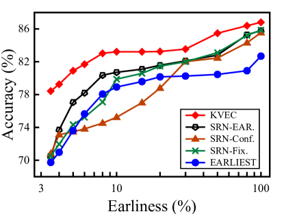
((a)) USTC-TFC2016

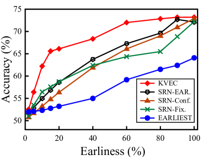
((b)) MovieLens-1M

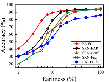
((c)) Traffic-FG

((d)) Traffic-App

Figure 3: Accuracy comparison

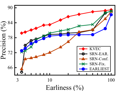
((a)) USTC-TFC2016

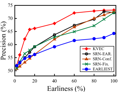
((b)) MovieLens-1M

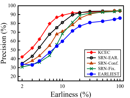
((c)) Traffic-FG

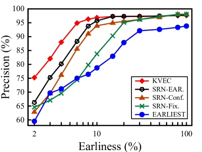
((d)) Traffic-App

Figure 4: Precision comparison

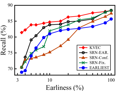
((a)) USTC-TFC2016

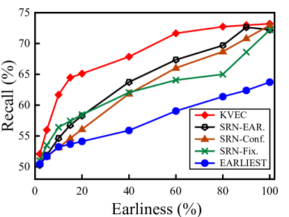
((b)) MovieLens-1M

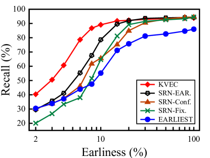
((c)) Traffic-FG

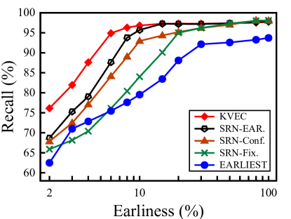
((d)) Traffic-App

Figure 5: Recall comparison

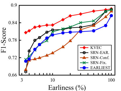
((a)) USTC-TFC2016

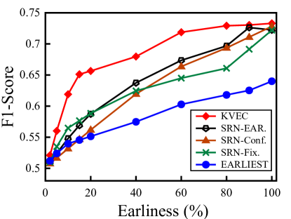
((b)) MovieLens-1M

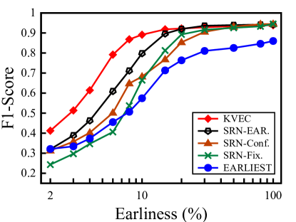
((c)) Traffic-FG

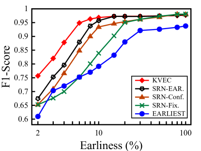
((d)) Traffic-App

Figure 6: F1-score comparison

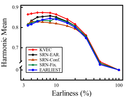
((a)) USTC-TFC2016

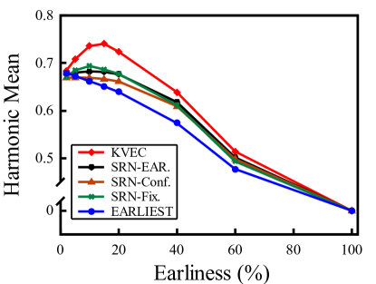
((b)) MovieLens-1M

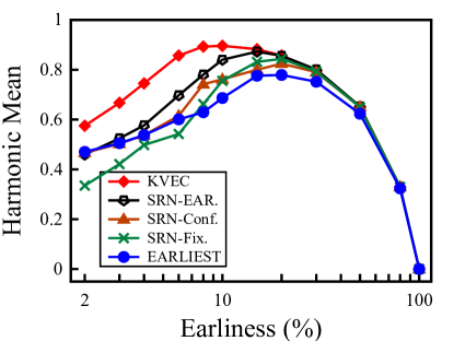
((c)) Traffic-FG

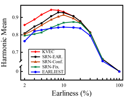
((d)) Traffic-App

Figure 7: HM comparison

Figures 3 to 6 depict the curves of classification performance vs. earliness of each early classification method on the four real-world datasets. We observe that the metrics increase as the earliness becomes large. This observation is consistent with our intuition, as more items are observed in a key-value sequence, we are more confident about its class label and hence achieve better classification performance. Comparing KVEC with other methods, we observe that, on all of real-world datasets, KVEC consistently achieves the highest accuracy than the others. This improvement is particularly notable in the early period, i.e., earliness is small. Specifically, when earliness is in the range of $2-8\%$, KVEC achieves accuracy improvements of $4.7\%$, $17.5\%$, and $6.4\%$ on the three traffic datasets, respectively, in comparison with the most competitive baseline SRN-EARLIEST; and achieves an average accuracy improvement of $7.8\%$ on the MovieLens-1M dataset than SRN-EARLIEST when the earliness is in the range of $10-40\%$. Similar performance improvements are observed for precision, recall, and F1 score. This observation demonstrates that our KVEC has a better classification performance than the other methods, especially when prediction earliness is crucial.

Furthermore, we observed that EARLIEST, despite being considered the state-of-the-art TSEC method, exhibits nearly the poorest performance on key-value sequence datasets. Even when the entire sequence is observed (i.e., earliness equals $100\%$), the accuracy of EARLIEST remains significantly lower than other methods. This disparity stems from the inherent differences between time series data and key-value sequence data, affirming our assertion that existing TSEC methods are not well-suited for key-value sequence data.

Figure 7 illustrates the relation between harmonic mean and earliness of each early classification method. On the four real-world datasets, we observe that the curves first increase and then drop as earliness increases. This is due to the property of harmonic mean in its definition. Similar to the observations in Fig. 3, on the four real-world datasets, KVEC generally performs better than the other methods, and the average improvements on the four datasets are about $2.9\%,5.3\%,14.0\%$, and $3.7\%$, respectively, with respect to the best among other baselines. This indicates that KVEC achieves a better balance between earliness and accuracy, compared to other baselines.

V-C Hyperparameter Sensitivity

Next, we study the sensitivity of the hyperparameters in KVEC, i.e., $\alpha$ and $\beta$, which regulate the weight of halting policy and time penalty to the overall loss function, respectively. We illustrate the hyperparameters’ effects on prediction accuracy and earliness on the Traffic-FG dataset in Fig. 8.

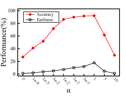
((a)) Effect of $\alpha$ on performance

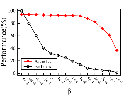
((b)) Effect of $\beta$ on performance

Figure 8: Hyperparameter sensitivity analysis.

In Fig. 8(a), we maintain $\beta$ at $10^{-4}$ and tune $\alpha$ within the range of $[0,10]$ to control the update weight of the halting policy. Instead, in Fig. 8(b), we set $\alpha$ to $0.1$ and tune $\beta$ within the range of $[-0.05,5]$ to control the intensity of the time delay penalty. We observe that $\alpha$ significantly impacts accuracy but has little effect on earliness; while $\beta$ primarily serves to balance prediction accuracy and earliness by penalizing halting time delay. According to this observation, in the experiments, we freeze $\alpha$ at $0.1$ and tune $\beta$ within the range of $[-0.05,5]$ to obtain the complete performance curve of KVEC.

V-D Ablation Study

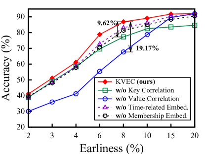
((a)) Effect on Accuracy

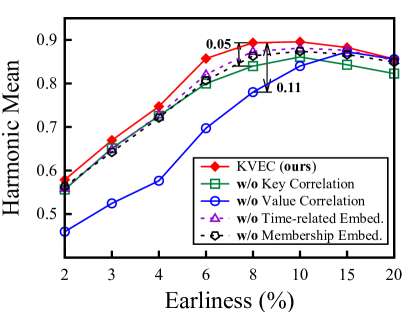
((b)) Effect on Harmonic Mean

Figure 9: Ablation study

We perform an ablation study to investigate the function of each component in KVEC. The experiments are conducted on the Traffic-FG dataset, and the results are shown in Fig. 9.

In the figure, “w/o Key Correlation” means that we remove the key correlation, only the value correlation is preserved in KVEC; “w/o Value Correlation” means that we completely remove the value correlation in KVEC, and treat each key-value sequence independently; “w/o Time-related Embed.” means that all time-related embeddings including relative position embedding and time embedding in the input embedding are completely removed; “w/o Membership Embed.” means that the membership embedding in input embedding is removed.

We have the following observations. First, the performance of the KVEC has the most significant slump after removing the value correlation. This confirms that the powerful performance of KVEC is mainly due to value correlations in a tangled key-value sequence. Meanwhile, removing the key correlation also harms the performance of KVEC. Second, the performance of KVEC without relative position embedding and time embedding performances drops slightly, which indicates that time-related information indeed can improve the quality of sequence representation learning and timing learning. Third, the performance of KVEC without the membership embedding also drops slightly, which indicates that distinguishing correlation information from different sequences is essential for learning a better sequence representation.

V-E Discussions

In this section, to better understand the proposed KVEC framework, we conduct a comprehensive qualitative analysis to answer the following research questions:

• RQ1: How does the KVRL module actually work, and does its attention mechanism indeed benefit early classification?

• RQ2: How does the halting policy work, and does the KVRL module effectively facilitates early halting?

• RQ3: What are the reliability and limitations of KVEC in practical application scenarios?

Attention mechanism in KVEC (RQ1). In the KVRL module, a pivotal design is a novel attention mechanism that leverages item correlations from both intra-sequence and inter-sequence. To answer RQ1, we quantify the attention distribution of KVRL module under various halting positions. In this experiment, we specifically employ the internal attention score and external attention score to represent the cumulative attention weights derived from key correlations and value correlations, respectively. We conduct this experiment using the Traffic-FG dataset and compare the attention scores and accuracy at various earliness, as depicted in Fig. 10.

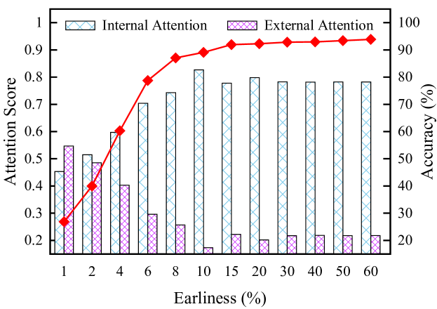
Figure 10: Distribution of attention score in various halting positions.

We observe that, the external attention score in the early time period (i.e., earliness is less than $10\%$) is higher than in the later time period. When more items in the sequence are observed, the external attention score generally decreases, and internal attention score progressively assumes dominance. This indicates that in early classification tasks, since intra-sequence data is insufficient, KVEC prioritizes exploring inter-sequence correlations to enhance sequence representations, thereby improving the earliness. In contrast, when sufficient data is observed, KVEC tends to focus on exploiting intra-sequence correlations to achieve higher accuracy.

Halting policy in KVEC (RQ2). In KVEC, a reinforcement learning-based halting policy is employed to control the timing of early classification. To answer RQ2, we compare the disparity between the halting positions predicted by the halting policy in KVEC and its variant (i.e., KVEC without value correlation) and the true halting positions within the Synthetic-Traffic dataset. The results are depicted in Fig. 11.

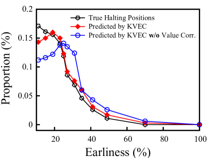
((a)) Early-stop subdataset

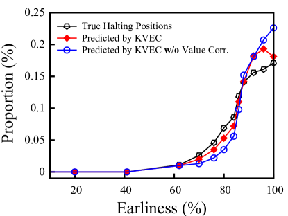
((b)) Late-stop subdataset

Figure 11: Distribution of halting positions predicted by different methods.

We observe that the distribution of halting positions in both early-stop data and late-stop data predicted by KVEC are closest to the distribution of true halting positions. This indicates that the halting policy within KVEC can accurately capture dynamic stopping signals, and proposed representation learning method (i.e., KVRL) indeed facilitates this ability.

Performance in practical applications (RQ3). In KVEC, multiple concurrent key-value sequences within a tangled key-value sequence are jointly modeled. In practical applications, the number of concurrent sequences in various scenarios is a primary factor affecting KVEC’s performance. To answer question RQ3, we conduct experiments on the Traffic-FG dataset, selecting diverse testing scenarios with varying numbers of concurrent key-value sequences $K$. The results are depicted in Fig. 12.

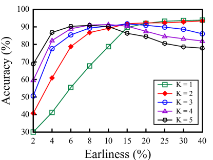
((a)) Accuracy vs. earliness

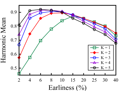
((b)) Harmonic mean vs. earliness

Figure 12: Effects of $K$ to performance of KVEC.

Our observations reveal that, in various testing scenarios, KVEC exhibits higher early classification accuracy at the early time period (i.e., earliness is less than $10\%$) when $K$ becomes larger. However, while at the later time period, KVEC performs worse when $K$ becomes larger. This demonstrates that in a more complex scenario, i.e., with a larger $K$, KVEC can exploit more inter-sequence correlations to enrich the sequence representation, but these inter-sequence correlations also inevitably introduce more noise information and lead to unstable performance. This phenomenon inspires us to find a more intelligent approach to leverage inter-sequence correlations in future work.

VI Conclusion

In this work, we formulate a novel tangled key-value sequence early classification problem, which has a wide range of applications in real world. We propose the KVEC framework to solve this problem. KVEC mainly consists of two steps, i.e., the key-value sequence representation learning, and the joint optimization of prediction accuracy and prediction earliness. The core idea behind KVEC is to leverage the rich intra- and inter-sequence correlations within the tangled key-value sequence to obtain an informative sequence representation. Through combining representation learning with timing learning, KVEC dynamically determines the optimal timing for early classification. Extensive experiments conducted on both real-world and synthetic datasets demonstrate that KVEC outperforms all alternative methods.

References

- [1] Wikipedia, “NetFlow,” https://en.wikipedia.org/wiki/NetFlow, 2022.
- [2] S. Yan, X. Chen, R. Huo, X. Zhang, and L. Lin, “Learning to build user-tag profile in recommendation system,” in ACM CIKM, 2020.
- [3] W. Zheng, C. Gou, L. Yan, and S. Mo, “Learning to classify: A flow-based relation network for encrypted traffic classification,” in WWW, 2020.
- [4] S. Rezaei and X. Liu, “Multitask learning for network traffic classification,” in ICCCN, 2020.
- [5] Y. Huang, G. G. Yen, and V. S. Tseng, “Snippet policy network for multi-class varied-length ECG early classification,” IEEE Transactions on Knowledge and Data Engineering (TKDE), vol. 35, pp. 1–14, 2022.
- [6] Y. Huang, G. G. Yen, and V. S. Tseng, “Snippet policy network V2: Knee-guided neuroevolution for multi-lead ECG early classification,” IEEE Transactions on Neural Networks and Learning Systems (TNNLS), pp. 1–15, 2022.
- [7] T. Hartvigsen, C. Sen, X. Kong, and E. Rundensteiner, “Recurrent halting chain for early multi-label classification,” in SIGKDD, 2020.
- [8] T. Hartvigsen, C. Sen, X. Kong, and E. Rundensteiner, “Adaptive-halting policy network for early classification,” in SIGKDD, 2019.
- [9] Wikipedia, “Internet traffic engineering,” https://en.wikipedia.org/wiki/Internet_traffic_engineering, 2022.
- [10] Z. Xu, M. Zhao, L. Liu, L. Xiao, X. Zhang, and B. Zhang, “Mixture of virtual-kernel experts for multi-objective user profile modeling,” in SIGKDD, 2022.
- [11] H. Fang, D. Zhang, Y. Shu, and G. Guo, “Deep learning for sequential recommendation: Algorithms, influential factors, and evaluations,” ACM Transactions on Information Systems (TOIS), vol. 39, pp. 1–42, 2020.
- [12] F. Lv, T. Jin, C. Yu, F. Sun, Q. Lin, K. Yang, and W. Ng, “SDM: Sequential deep matching model for online large-scale recommender system,” in ACM CIKM, 2019.
- [13] C. Liu, L. He, G. Xiong, Z. Cao, and Z. Li, “FS-Net: A flow sequence network for encrypted traffic classification,” in INFOCOM, 2019, pp. 1171–1179.
- [14] P. Sirinam, N. Mathews, M. S. Rahman, and M. Wright, “Triplet fingerprinting: More practical and portable website fingerprinting with n-shot learning,” in CCS, 2019, pp. 1131–1148.
- [15] J. Hayes and G. Danezis, “k-fingerprinting: A robust scalable website fingerprinting technique,” in 25th USENIX Security Symposium (USENIX Security), 2016, pp. 1187–1203.
- [16] C. Xu, J. Shen, and X. Du, “A method of few-shot network intrusion detection based on meta-learning framework,” IEEE Transactions on Information Forensics and Security (TIFS), vol. 15, pp. 3540–3552, 2020.
- [17] Y. Fu, H. Xiong, X. Lu, J. Yang, and C. Chen, “Service usage classification with encrypted internet traffic in mobile messaging apps,” IEEE Transactions on Mobile Computing (TMC), vol. 15, pp. 2851–2864, 2016.
- [18] J. Liu, Y. Fu, J. Ming, Y. Ren, L. Sun, and H. Xiong, “Effective and real-time in-app activity analysis in encrypted internet traffic streams,” in SIGKDD, 2017.
- [19] X. Ma, J. Qu, J. Li, J. C. Lui, Z. Li, and X. Guan, “Pinpointing hidden iot devices via spatial-temporal traffic fingerprinting,” in INFOCOM, 2020, pp. 894–903.
- [20] X. Ma, J. Qu, J. Li, J. C. Lui, Z. Li, W. Liu, and X. Guan, “Inferring hidden iot devices and user interactions via spatial-temporal traffic fingerprinting,” IEEE/ACM Transactions on Networking (TON), vol. 30, pp. 394–408, 2021.
- [21] A. Gupta, H. P. Gupta, B. Biswas, and T. Dutta, “Approaches and applications of early classification of time series: A review,” IEEE Transactions on Artificial Intelligence, vol. 1, pp. 47–61, 2020.
- [22] T. Hartvigsen, W. Gerych, J. Thadajarassiri, X. Kong, and E. Rundensteiner, “Stop&Hop: Early classification of irregular time series,” in ACM CIKM, 2022.
- [23] A. Gupta, H. P. Gupta, B. Biswas, and T. Dutta, “A fault-tolerant early classification approach for human activities using multivariate time series,” IEEE Transactions on Mobile Computing (TMC), vol. 20, pp. 1747–1760, 2020.
- [24] L. Ye and E. Keogh, “Time series shapelets: a new primitive for data mining,” in SIGKDD, 2009.
- [25] M. F. Ghalwash and Z. Obradovic, “Early classification of multivariate temporal observations by extraction of interpretable shapelets,” BMC bioinformatics, vol. 13, pp. 1–12, 2012.
- [26] M. F. Ghalwash, V. Radosavljevic, and Z. Obradovic, “Extraction of interpretable multivariate patterns for early diagnostics,” in ICDM, 2013, pp. 201–210.
- [27] Z. Xing, J. Pei, and P. S. Yu, “Early prediction on time series: A nearest neighbor approach,” in IJCAI, 2009, pp. 1297–1302.
- [28] Z. Xing, J. Pei, P. S. Yu, and K. Wang, “Extracting interpretable features for early classification on time series,” in SDM, 2011, pp. 247–258.
- [29] Z. Xing, J. Pei, and P. S. Yu, “Early classification on time series,” Knowledge and information systems, vol. 31, pp. 105–127, 2012.
- [30] G. He, Y. Duan, R. Peng, X. Jing, T. Qian, and L. Wang, “Early classification on multivariate time series,” Neurocomputing, vol. 149, pp. 777–787, 2015.
- [31] P. Schäfer and U. Leser, “Teaser: early and accurate time series classification,” Data mining and knowledge discovery (DMKD), vol. 34, pp. 1336–1362, 2020.
- [32] U. Mori, A. Mendiburu, E. Keogh, and J. A. Lozano, “Reliable early classification of time series based on discriminating the classes over time,” Data mining and knowledge discovery (DMKD), vol. 31, pp. 233–263, 2016.
- [33] U. Mori, A. Mendiburu, S. Dasgupta, and J. A. Lozano, “Early classification of time series by simultaneously optimizing the accuracy and earliness,” IEEE Transactions on Neural Networks and Learning Systems (TNNLS), vol. 29, pp. 4569–4578, 2017.
- [34] H.-S. Huang, C.-L. Liu, and V. S. Tseng, “Multivariate time series early classification using multi-domain deep neural network,” in DSAA, 2018.
- [35] M. Rußwurm, N. Courty, R. Emonet, S. Lefèvre, D. Tuia, and R. Tavenard, “End-to-end learned early classification of time series for in-season crop type mapping,” ISPRS Journal of Photogrammetry and Remote Sensing, vol. 196, pp. 445–456, 2023.
- [36] A. F. Ebihara, T. Miyagawa, K. Sakurai, and H. Imaoka, “Sequential density ratio estimation for simultaneous optimization of speed and accuracy,” in ICLR, 2020.
- [37] M. Rußwurm, S. Lefevre, N. Courty, R. Emonet, M. Körner, and R. Tavenard, “End-to-end learning for early classification of time series,” Journal of Photogrammetry and Remote Sensing, vol. 196, pp. 445–456, 2019.
- [38] C. Martinez, G. Perrin, E. Ramasso, and M. Rombaut, “A deep reinforcement learning approach for early classification of time series,” in EUSIPCO, 2018, pp. 2030–2034.
- [39] C. Martinez, E. Ramasso, G. Perrin, and M. Rombaut, “Adaptive early classification of temporal sequences using deep reinforcement learning,” Knowledge-Based Systems (KBS), vol. 190, p. 105290, 2020.
- [40] L. Guo, H. Yin, Q. Wang, T. Chen, A. Zhou, and N. Q. V. Hung, “Streaming session-based recommendation,” in SIGKDD, 2019.
- [41] M. Choi, J. Kim, J. Lee, H. Shim, and J. Lee, “Session-aware linear item-item models for session-based recommendation,” in WWW, 2021, pp. 2186–2197.
- [42] M. Shen, J. Zhang, L. Zhu, K. Xu, and X. Du, “Accurate decentralized application identification via encrypted traffic analysis using graph neural networks,” IEEE Transactions on Information Forensics and Security (TIFS), vol. 16, pp. 2367–2380, 2021.
- [43] A. Vaswani, N. Shazeer, N. Parmar, J. Uszkoreit, L. Jones, A. N. Gomez, L. Kaiser, and I. Polosukhin, “Attention is all you need,” in Advances in neural information processing systems (NIPS), 2017.
- [44] S. Hochreiter and J. Schmidhuber, “Long short-term memory,” Supervised sequence labelling with recurrent neural networks, vol. 9, p. 1735–1780, 1997.
- [45] R. S. Sutton and A. G. Barto, Reinforcement Learning: An Introduction. Richard S. Sutton and Andrew G. Barto, 2020, ch. Policy Gradient Methods, pp. 321–337.
- [46] W. Wang, M. Zhu, X. Zeng, X. Ye, and Y. Sheng, “Malware traffic classification using convolutional neural network for representation learning,” in ICoIN, 2017.
- [47] MovieLens, “Movielens 1M dataset,” https://grouplens.org/datasets/movielens/1m/, 2003.
- [48] S. Rezaei and X. Liu, “Deep learning for encrypted traffic classification: An overview,” IEEE communications magazine, vol. 57, pp. 76–81, 2019.
- [49] S. Ma, L. Sigal, and S. Sclaroff, “Learning activity progression in LSTMs for activity detection and early detection,” in CVPR, 2016, pp. 1942–1950.
- [50] N. Parrish, H. S. Anderson, M. R. Gupta, and D. Y. Hsiao, “Classifying with confidence from incomplete information,” The Journal of Machine Learning Research, vol. 14, pp. 3561–3589, 2013.