SNSeg: An R Package for Time Series Segmentation via Self-Normalization

Abstract

Time series segmentation aims to identify potential change-points in a sequence of temporally dependent data, so that the original sequence can be partitioned into several homogeneous subsequences. It is useful for modeling and predicting non-stationary time series and is widely applied in natural and social sciences. Existing segmentation methods primarily focus on only one type of parameter changes such as mean and variance, and they typically depend on laborious tuning or smoothing parameters, which can be challenging to choose in practice. The self-normalization based change-point estimation framework SNCP by Zhao et al. (2022), however, offers users more flexibility and convenience as it allows for change-point estimation of different types of parameters (e.g. mean, variance, quantile and autocovariance) in a unified fashion, and requires effortless tuning. In this paper, the R package SNSeg is introduced to implement SNCP for segmentation of univariate and multivariate time series. An extension of SNCP, named SNHD, is also designed and implemented for change-point estimation in the mean vector of high-dimensional time series. The estimated change-points as well as segmented time series are available with graphical tools. Detailed examples of SNSeg are given in simulations of multivariate autoregressive processes with change-points.

1  Introduction

Time series segmentation, also known as change-point estimation in time series, has become increasingly popular in various fields such as statistics, bioinformatics, climate science, economics, finance, signal processing, epidemiology, among many others. As a result, numerous methods have been proposed to address different types of change-point estimation problems under various settings. This in turn leads to the development of many R packages for their implementation.

Here, we list some commonly used and influential packages for change-point analysis in the R programming language. The package strucchange (Zeileis et al., 2002) employs algorithms proposed by Zeileis et al. (2003) to identify structural changes in linear regression models. The package changepoint (Killick and Eckley, 2014) provides numerous methods for estimating change-points in a univariate time series, containing the Binary Segmentation (BS) and the pruned exact linear time (PELT) algorithm as described in Killick et al. (2012), and the segment neighbourhoods algorithm in Auger and Lawrence (1989). The package mosum (Meier et al., 2021) executes the moving sum (MOSUM) procedure introduced by Eichinger and Kirch (2018) for univariate time series. It can implement MOSUM with a single bandwidth parameter and also allows multiple bandwidths via either bottom-up merging or localized pruning. The package cpss (Wang and Zou, 2023) focuses on change-point estimation in various generalized linear models utilizing the sample-split strategy proposed by Zou et al. (2020). We note that there are also packages targeting nonparametric distributional changes, e.g. the package ecp (James and Matteson, 2014) and cpm (Ross, 2015).

However, the aforementioned methods, as well as their implementation packages, are subject to certain limitations when applied to change-point estimation in multivariate time series. First, most packages only provide functions to detect specific types of changes (e.g. mean or variance). Although it may be possible to modify these functions to cover other types of changes (e.g. quantiles), such a generalization is usually not easy and requires non-trivial effort. This means that for the same dataset, different methods or substantial modifications to the existing codes may be required for estimating different types of changes, which may incur inconvenience of implementation for practitioners. Second, many packages implement methods that assume temporal independence among data, which may not be realistic in practice, and thus may suffer from issues such as false positive detections.

Recently, Zhao et al. (2022) have developed a new framework called self-normalization based change-point estimation (SNCP) to overcome the above limitations. The most appealing feature of SNCP is its versatility as it allows for change-point estimation in a broad class of parameters (such as mean, variance, correlation, quantile and their combinations) in a unified fashion. The basic idea of SNCP is to augment the conventional cumulative sum (CUSUM) statistics with the technique called self-normalization (SN). SN is originally introduced by Shao (2010) for confidence interval construction of a general parameter in the stationarity time series setting, and is later extended to change-point testing by Shao and Zhang (2010). It can bypass the issue of bandwidth selection in the consistent long-run variance estimation. See Shao (2015) for a review. SNCP is fully nonparametric, robust to temporal dependence and applicable universally for various parameters of interest for a multivariate time series. Furthermore, based on a series of carefully designed nested local-windows, SNCP can isolate each true change-point adaptively and achieves the goal of multiple change-point estimation with respectable detection power and estimation accuracy.

In this paper, we introduce the R package SNSeg (Sun et al., 2023), which implements the SNCP framework in Zhao et al. (2022) for univariate and multivariate time series segmentation. This is achieved by the functions SNSeg_Uni() and SNSeg_Multi(), respectively. Another contribution of this paper is to extend the SNCP framework to change-point estimation in the mean vector of a high-dimensional time series. Since SNCP is only applicable to fixed-dimensional time series, a new procedure based on U-statistics (Wang et al., 2022), termed as SNHD, is proposed by modifying the original SNCP in Zhao et al. (2022). The implementation of SNHD is available through the function SNSeg_HD(). Graphical options are also allowed for plotting the estimated change-points and associated test statistics.

The rest of the paper is organized as follows. We first provide the background of SN based statistics and the SNCP/SNHD procedures for change-point estimation in Section 2. In Section 3, we demonstrate the core functions of the package SNSeg by various examples of change-point estimation problems. Additional simulation results and comparison with existing packages are provided in Section 4. Section 5 concludes.

2  SNCP Framework

This section gives necessary statistical backgrounds of SNCP in change-point estimation problems. We first demonstrate how an SN based CUSUM test statistic works for estimating a single change-point, and then introduce the nested local-window based SNCP algorithm for multiple change-point estimation. The extension of SNCP to change-point estimation in high-dimensional mean problem is also provided and we term the related algorithm as SNHD. The issue of how to choose tuning parameters is also discussed.

2.1  Single Change-Point Estimation

Let $\{Y_{t}\}^{n}_{t=1}$ be a sequence of multivariate time series of dimension $p$, which is assumed to be fixed for now. We aim to detect whether there is a change-point in the quantities $\{\theta_{t}\}^{n}_{t=1}$ defined by $\theta_{t}=\theta(F_{t})\in\mathbb{R}^{d}$, where $F_{t}$ denotes the distribution function of $Y_{t}$, and $\theta(\cdot)$ is a general functional such as mean, variance, auto-covariance, quantiles, etc. More specifically, if there is no change-point, then

$$\theta_{1}=\cdots=\theta_{n}.$$ (1)

Otherwise, we assume there is an unknown change-point $k^{*}\in\{1,\cdots,n-1\}$ defined by

$$\theta_{1}=\cdots=\theta_{k^{*}}\neq\theta_{k^{*}+1}=\cdots=\theta_{n},$$ (2)

and our interest is to recover the location $k^{*}$.

The above setting allows for at most one change-point in $\{\theta_{t}\}^{n}_{t=1}$. A commonly used statistic for testing the existence of change-points is based on the CUSUM process, defined by

$$D_{n}(k)=\frac{k(n-k)}{n^{3/2}}\left(\hat{\theta}_{1,k}-\hat{\theta}_{k+1,n}\right),~{}~{}k\in\{1,2,\cdots,n-1\},$$ (3)

where for any $1\leq a<b\leq n$, $\hat{\theta}_{a,b}=\theta(\hat{F}_{a,b})$ estimates the model parameter with $\hat{F}_{a,b}$ being the empirical distribution of $\{Y_{t}\}_{t=a}^{b}$. For example, when $\theta(\cdot)$ is the mean functional, it can be shown that

$$D_{n}(k)=\frac{1}{\sqrt{n}}\sum_{t=1}^{k}(Y_{t}-\bar{Y}),\quad\bar{Y}=n^{-1}\sum_{t=1}^{n}Y_{t}.$$

The CUSUM process in (3) sequentially compares the estimates before and after a time point $k$, and its norm is expected to attain the maximum when $k=k^{*}$. Intuitively, if (1) holds, then $D_{n}(k)$ should fluctuate around zero; otherwise if (2) holds, then $\hat{\theta}_{1,k}$ and $\hat{\theta}_{k+1,n}$ are consistent estimators for $\theta_{1}$ and $\theta_{n}$, respectively at $k=k^{*}$, and the resulting contrast $\|D_{n}(k^{*})\|$ would be most informative about the change signal $\Delta_{n}=\theta_{k^{*}+1}-\theta_{k^{*}}$. Therefore, it is natural to estimate the change-point location via

$$\tilde{k}=\arg\max_{k=1,\cdots,n-1}\|D_{n}(k)\|^{2}.$$ (4)

However, analyzing the asymptotic distribution of CUSUM process $\{D_{n}(\lfloor nr\rfloor)\}_{r\in[0,1]}$ for time series data is difficult, as it typically depends on a nuisance parameter called long-run variance (Newey and West, 1987; Andrews, 1991). As mentioned before, the estimation of long-run variance is quite challenging even in a stationary time series, let alone the scenario when a change-point is present.

To bypass this issue, Zhao et al. (2022) propose to estimate the change-point via the self-normalized version of (4), i.e.

$$\hat{k}=\arg\max_{k=1,\cdots,n-1}T_{n}(k),\quad T_{n}(k)=D_{n}(k)^{\prime}V^{-1}_{n}(k)D_{n}(k),$$ (5)

where

$$V_{n}(k)=\sum_{i=1}^{k}\frac{i^{2}(k-i)^{2}}{n^{2}k^{2}}(\hat{\theta}_{1,i}-\hat{\theta}_{i+1,k})^{\otimes 2}+\sum_{i=k+1}^{n}\frac{(n-i+1)^{2}(i-k-1)^{2}}{n^{2}(n-k)^{2}}(\hat{\theta}_{i,n}-\hat{\theta}_{k+1,i-1})^{\otimes 2},$$ (6)

is defined as the self-normalizer of $D_{n}(k)$ with $a^{\otimes 2}=aa^{\top}$ for a vector $a.$ The self-normalizer $V_{n}(k)$ is proportional to long run variance, which gets canceled out in the limiting null distribution of $T_{n}(k)$. Thus, the testing/estimation of a single change-point is completely free of tuning parameters.

In practice, we may not know whether the series $\{\theta_{t}\}_{t=1}^{n}$ contains a change-point or not, so a testing step is called for prior to the estimation step. Formally speaking, given a pre-specified threshold $K_{n}$, we declare the existence of a change-point when

$$SN_{n}:=\max_{k=1,\cdots,n-1}T_{n}(k)>K_{n},$$

and then estimate the single change-point via (5). Otherwise, if $SN_{n}$ is below the threshold $K_{n}$, we declare no change-points.

2.2  Multiple Change-Point Estimation

Section 2.1 introduces how SNCP works in the single change-point setting. In this section, we further discuss its implementation for multiple change-point estimation. Compared with the single change-point setting, the main difficulty of multiple change-point estimation lies in how to isolate one change-point from another. In SNCP, this is achieved by a nested local-window approach.

We first introduce some notations. Assume there are $m_{0}\geq 0$ unknown number of change-points with $k_{0}=0<k_{1}<\cdots<k_{m_{0}}<n=k_{m_{0}+1}$ that partition $Y_{t}$ into $m_{0}+1$ stationary segments with constant quantity of interest $\theta^{(i)}$ in the $i$th segment, for $i=1,\cdots,m_{0}+1$. In other words,

$$\theta_{t}=\theta^{(i)},~{}~{}k_{i-1}+1\leq t\leq k_{i},~{}\text{for}~{}i=1,\cdots,m_{0}+1.$$

Similar to the single change-point estimation framework, for $1\leq t_{1}<k<t_{2}\leq n$, we define an SN based test statistic

$$T_{n}(t_{1},k,t_{2})=D_{n}(t_{1},k,t_{2})^{\prime}V_{n}^{-1}(t_{1},k,t_{2})D_{n}(t_{1},k,t_{2}),$$ (7)

where $D_{n}(t_{1},k,t_{2})=\frac{(k-t_{1}+1)(t_{2}-k)}{(t_{2}-t_{1}+1)^{3/2}}(\hat{\theta}_{t_{1},k}-\hat{\theta}_{k+1,t_{2}})$, $V_{n}(t_{1},k,t_{2})=L_{n}(t_{1},k,t_{2})+R_{n}(t_{1},k,t_{2})$ and

$$L_{n}(t_{1},k,t_{2})=\sum_{i=t_{1}}^{k}\frac{(i-t_{1}+1)^{2}(k-i)^{2}}{(t_{2}-t_{1}+1)^{2}(k-t_{1}+1)^{2}}(\hat{\theta}_{t_{1},i}-\hat{\theta}_{i+1,k})^{\otimes 2},$$

$$R_{n}(t_{1},k,t_{2})=\sum_{i=k+1}^{t_{2}}\frac{(t_{2}-i+1)^{2}(i-1-k)^{2}}{(t_{2}-t_{1}+1)^{2}(t_{2}-k)^{2}}(\hat{\theta}_{i,t_{2}}-\hat{\theta}_{k+1,i-1})^{\otimes 2}.$$

Here $T_{n}(t_{1},k,t_{2})$ plays the same role as $T_{n}(k)$ in (5), except for the fact that it is defined on the subsample $\{Y_{t}\}_{t=t_{1}}^{t_{2}}$. In other words, $T_{n}(t_{1},k,t_{2})=T_{n}(k)$ if $t_{1}=1$ and $t_{2}=n$.

We now combine the SN framework with a nested local-window segmentation algorithm in Zhao et al. (2022) for multiple change-point estimation. For each $k$, instead of using the global statistic $T_{n}(1,k,n)$ which is computed with all observations, we compute a maximal SNCP test statistic based on a collection of nested windows covering $k$. Specifically, we fix a small trimming parameter $\epsilon\in(0,1/2)$ and define the window size $h=\lfloor{n\epsilon}\rfloor$. For each $k=h,\cdots,n-h$, we define the nested local-window set $H_{1:n}(k)$ as

$$H_{1:n}(k)=\{(t_{1},t_{2})|t_{1}=k-j_{1}h+1,j_{1}=1,\cdots,\lfloor{k/h}\rfloor;t_{2}=k+j_{2}h,j_{2}=1,\cdots,\lfloor{(n-k)/h}\rfloor.\}$$ (8)

Note that for $k<h$ and $k>n-h$, we have $H_{1:n}(k)=\emptyset$. In Figure 1, we plot a graphical illustration of the nested local-windows in $H_{1:n}(k)$, where local windows are constructed by combining every pair of the red left bracket ${\color[rgb]{1,0,0}[}$ and the blue right bracket ${]}$.

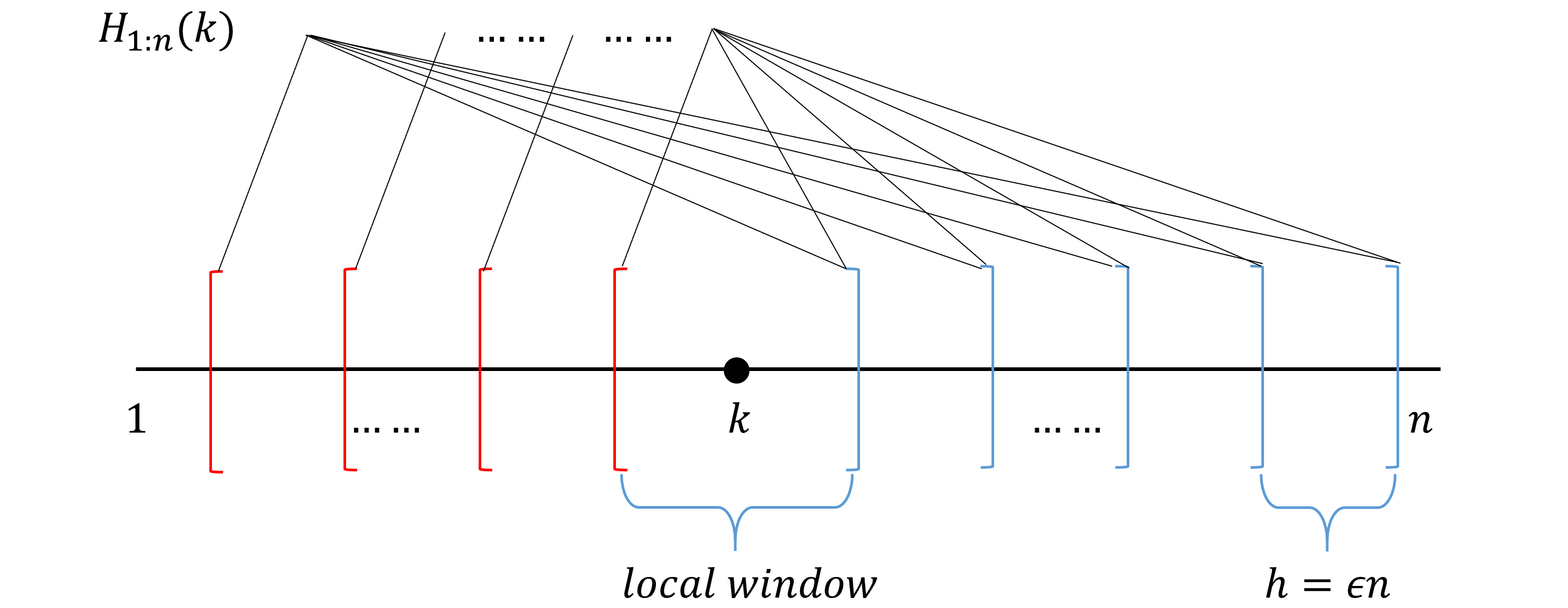
Figure 1: Graphical illustration of the nested local-windows in $H_{1:n}(k)$. Each pair of the red left bracket ${\color[rgb]{1,0,0}[}$ and the blue right bracket ${]}$ represents a local-window in $H_{1:n}(k)$.

For each $k=1,\cdots,n-1$, based on its nested local-window set $H_{1:n}(k)$, we define a maximal SN test statistic such that

$$T_{1,n}(k)=\max_{(t_{1},t_{2})\in H_{1:n}(k)}T_{n}(t_{1},k,t_{2}),$$ (9)

where we set $\max_{(t_{1},t_{2})\in\emptyset}T_{n}(t_{1},k,t_{2})=0$.

Intuitively, with a sufficiently small trimming $\epsilon$, the nested local-window framework ensures that for a true change-point location, say $k^{*}$, there exists some local window set denoted by $(t_{1}^{*},t_{2}^{*})$ containing $k^{*}$ as the only change-point. In other words, $k^{*}$ is isolated by the interval $(t_{1}^{*},t_{2}^{*})$ so that the procedure in the single change-point scenario as Section 2.1 can be applied. This suggests that for at least one pair of $(t_{1},t_{2})$ in $H_{1:n}(k)$, $T_{n}(t_{1},k^{*},t_{2})$ is large. The detection power is further enhanced by taking the maximum of these test statistics.

Based on the maximal test statistic $T_{1,n}(k)$ and a pre-specified threshold $K_{n}$, SNCP proceeds as follows. Starting with the full sample $\{Y_{t}\}_{t=1}^{n}$, we calculate $T_{1,n}(k),k=1,\cdots,n.$ Given that $\max_{k=1,\ldots,n}T_{n}(k)\leq K_{n}$, SNCP declares no change-point. Otherwise, SNCP sets $\widehat{k}=\arg\max_{k=1,\ldots,n}T_{1,n}(k)$ and we recursively perform SNCP on the subsample $\{Y_{t}\}_{t=1}^{\widehat{k}}$ and $\{Y_{t}\}_{t=\widehat{k}+1}^{n}$ until no change-point is declared. Denote $W_{s,e}=\bigl{\{}(t_{1},t_{2})\big{|}s\leq t_{1}<t_{2}\leq e\bigl{\}}$ and $H_{s:e}(k)=H_{1:n}(k)\bigcap W_{s,e}$, which is the nested window set of $k$ on the subsample $\{Y_{t}\}_{t=s}^{e}$. Define the subsample maximal SN test statistic as $T_{s,e}(k)=\max\limits_{(t_{1},t_{2})\in H_{s:e}(k)}T_{n}(t_{1},k,t_{2}).$ Algorithm 1 states the formal description of SNCP in multiple change-points estimation.

We note that SNCP shares some similarity with binary segmentation (BS) in the sense that both algorithms search for change-points in a sequential fashion. However, they are also quite different. In particular, the SN test statistic in SNCP is computed over a set of nested local-windows instead of over a single interval. In contrast, in the classical change-point literature, BS is usually coupled with a global CUSUM statistic computed over the entire dataset $[1,n]$. As is documented in the literature (Shao, 2010), the main drawback of BS is its power loss under non-monotonic change, which is caused by the use of the global CUSUM statistic coupled with the sequential search. However, due to the use of the nested local-window based SN test statistic, SNCP does not suffer from this power loss phenomenon as long as $\epsilon$ is chosen to be smaller than the minimum spacing between two change-points. On the other hand, due to the sequential search nature, both SNCP and BS may encounter the multiple testing problem. In addition, their power may be lesser compared to a global search algorithm, such as dynamic programming or PELT, which is again due to the sequential nature of the search algorithm.

Input: Time series $\{Y_{t}\}_{t=1}^{n}$, threshold $K_{n}$, window size $h=\lfloor n\epsilon\rfloor$

Output: Estimated change-points $\widehat{\mathbf{k}}=(\hat{k}_{1},\cdots,\hat{k}_{\hat{m}})$

Initialization: SNCP($1,n,K_{n},h$), $\widehat{\mathbf{k}}=\emptyset$

Procedure: SNCP($s,e,K_{n},h$)

if $e-s+1<2h$ then

       stop

else

       $\hat{k}^{*}=\arg\max_{k=s,\cdots,e}T_{s,e}(k)$;

      if $T_{s,e}(\hat{k}^{\ast})\leq K_{n}$ then

             stop

      else

             $\widehat{\mathbf{k}}=\widehat{\mathbf{k}}\cup\hat{k}^{\ast}$;

            run SNCP($s,\hat{k}^{\ast},K_{n},h$) and SNCP($\hat{k}^{\ast}+1,e,K_{n},h$);

       end if

      

end if

Algorithm 1 SNCP procedures for multiple change-point estimation

2.3  Multiple Change-Point Estimation for High-Dimensional Mean

In this section, we modify the SNCP framework in Section 2.2 to design a new algorithm called SNHD for multiple change-point estimation in the mean vector of a high-dimensional time series.

Different from the subsample test statistic $T_{n}(t_{1},k,t_{2})$ used in SNCP for a low-dimensional time series, SNHD is designed based on the high-dimensional U-statistic proposed by Wang et al. (2022). Given a $p$-dimensional time series $\{Y_{t}\}_{t=1}^{n}$, we define the subsample contrast statistic as

$$D_{n}^{U}(t_{1},k,t_{2})=\sum_{\begin{subarray}{c}t_{1}\leq j_{1},j_{3}\leq k\\ j_{1}\neq j_{3}\end{subarray}}\sum_{\begin{subarray}{c}k+1\leq j_{2},j_{4}\leq t_{2}\\ j_{2}\neq j_{4}\end{subarray}}(Y_{j_{1}}-Y_{j_{2}})^{\top}(Y_{j_{3}}-Y_{j_{4}}).$$ (10)

Note that $D_{n}^{U}(t_{1},k,t_{2})$ is a two-sample U-statistic estimating the squared $L_{2}$-norm of the difference between the means of $\{Y_{t}\}_{t=t_{1}}^{k}$ and $\{Y_{t}\}_{t=k+1}^{t_{2}}$ (up to some normalizing constant), and therefore targets dense changes in high-dimensional mean. The statistic in (10) is only applicable to high-dimensional time series with temporal independence, and in the presence of temporal dependence, a trimming parameter needs to be introduced to alleviate the bias due to serial dependence; see Wang et al. (2022). Define the self-normalizer as

$$V_{n}^{U}(t_{1},k,t_{2})=\frac{1}{n}\Big{[}\sum_{t=t_{1}+1}^{k-2}D_{n}^{U}(t_{1},t,k)^{2}+\sum_{t=k+2}^{t_{2}-2}D_{n}^{U}(k+1,t,t_{2})^{2}\Big{]}.$$ (11)

The subsample SNHD test statistic at time point $k$, in the same spirit as (9), is defined as

$$T_{1,n}^{U}(k)=\max_{(t_{1},t_{2})\in H_{1:n}(k)}T_{n}^{U}(t_{1},k,t_{2}),\quad T_{n}^{U}(t_{1},k,t_{2})=D_{n}^{U}(t_{1},k,t_{2})^{2}/V_{n}^{U}(t_{1},k,t_{2}),$$ (12)

where $H_{1:n}(k)$ is the nested local-window set defined in (8). With a pre-specified threshold $K_{n}^{U}$, a change-point is detected at $\hat{k}=\arg\max_{k=1,\cdots,n}T_{1,n}^{U}(k)$ if $\max_{k=1,\cdots,n}T_{1,n}^{U}(k)$ is above $K_{n}^{U}$. For multiple change-point estimation, SNHD proceeds similarly as SNCP in Algorithm 1.

2.4  Choice of Trimming Parameter $\epsilon$ and Threshold $K_{n}$

For practical implementation of SNCP and SNHD, there are still two tuning parameters that one has to choose, namely the trimming parameter $\epsilon$ and the change-point detection threshold $K_{n}$. The choice of $\epsilon$ reflects one’s belief of the minimum (relative) spacing between two consecutive change-points. This is usually set to be a small constant such as 0.05, 0.10, 0.15. The theoretical validity of our approach requires the minimum spacing between change-points to be of order $O(n)$, and opting for an overly small value of $\epsilon$ may result in sub-optimal performance in finite sample as the nested local-window may not contain sufficient observations. On the other hand, an overly large value of $\epsilon$ may increase the potential risk of under-estimating change-points if $\epsilon$ is larger than the minimum spacing between two true change-points. In practice, we recommend using 0.05 as a default value when no prior knowledge of minimum spacing between change-points is available.

A nice feature of using SN is that the limiting distributions for SNCP or SNHD under the no change-point scenario are pivotal and furthermore reflect the impact of the choice of $\epsilon$, see Theorem 3.1 in Zhao et al. (2022), and Section S.2.9 in Zhao et al. (2021), respectively. Since $K_{n}$ and $K_{n}^{U}$ are used to balance one’s tolerance of type-I and type-II errors, this implies that we can choose $K_{n}$ and $K_{n}^{U}$ as the $q\times 100\%$ quantiles (i.e. the critical value) of the limiting null distribution with $q$ typically set as 0.9, 0.95, 0.99. The threshold value $K_{n}$ also increases with the dimension of the quantity $\theta$, and we refer to Table 1 in Zhao et al. (2022) for details. In the SNSeg package, we offer users a wide range of $\epsilon$ and $q$ to choose from. Details are given in the following section.

In Section 4.1, we further conduct a sensitivity analysis, which suggests that the performance of SNCP in general is robust w.r.t. the choice of $(\epsilon,K_{n})$.

3  The SNSeg Package

In this section, we introduce the functions within the SNSeg package for multiple change-point estimation. In particular, SNSeg_Uni() in Section 3.1 implements the SNCP procedure of change-point estimation for a univariate time series with changes in a single or multiple parameters, such as mean, variance, auto-correlations, quantiles or even their combinations. It can also be implemented for detecting change-points in other quantities, with a user-defined function as input. The function SNSeg_Multi() in Section 3.2 utilizes the SNCP algorithm for change-point estimation in mean or covariance matrix of a multivariate time series. In Section 3.3, the function SNSeg_HD() estimates change-points in mean of a high-dimensional time series using the SNHD procedure. In addition to these major functions for change-point estimation, we further introduce max_SNsweep() in Section 3.4, which helps obtain the SN test statistics and create a segmentation plot based on the output of the above functions. Followed by the graphical options, the function SNSeg_estimate() generates parameter estimates within each segment separated by the estimated change-points.

3.1  SNCP for Univariate Time Series

For a univariate time series, change-point estimation in a single or multiple functionals can be implemented through the function SNSeg_Uni(). This function is also capable of detecting change-points associated with the change in correlation between bivariate time series. The R code is given as:

SNSeg_Uni(ts, paras_to_test, confidence = 0.9, grid_size_scale = 0.05,grid_size = NULL, plot_SN = TRUE, est_cp_loc = TRUE)It takes the following input arguments.

• ts: Input time series $\{Y_{t}\}_{t=1}^{n}$, i.e., a univariate time series expressed as a numeric vector with length $n$. However, when the argument paras_to_test is specified as bivcor, which stands for the correlation between bivariate time series, the input ts must be an $n\times 2$ matrix.

• paras_to_test: The parameters that SNCP aims to examine, which are presented as a string, a number, a combination of both, or a user-defined function that defines a specific functional. Available options of paras_to_test include:

  • "mean": The function performs change-point estimation on the mean of the time series.

  • "variance": The function performs change-point estimation on the variance.

  • "acf": The function performs change-point estimation on the autocorrelation of order 1.

  • "bivcor": The function performs change-point estimation on the bivariate correlation.

  • A numeric quantile value within the range (0,1): The function performs change-point estimation on the quantile level specified by the numeric value.

  • A vector containing characters "mean", "variance", "acf", and one or more numerical quantile levels. Therefore, SNSeg_Uni() is capable of estimating change-points in either a single parameter or a combination of multiple parameters.

  • A user-defined R function that returns a numeric value. Existing functions in R such as $\texttt{mean}()$ and $\texttt{var}()$ can also be used. This option provides additional flexibility for the users to define a specific functional that they are interested in and is not covered by our built-in options. The input argument paras_to_test should possess the form of function(...){}.

• confidence: A numeric value that specifies the confidence level of the SN test. Available choices of confidence levels contain 0.9, 0.95, 0.99, 0.995 and 0.999. It automatically obtains the threshold ($K_{n}$, the critical value) corresponding to the input confidence level. The default value of confidence is set at 0.9.

• grid_size_scale: A numeric value that specifies the trimming parameter $\epsilon$ and only in use if grid_size = NULL. Available choices include 0.05, 0.06, 0.07, 0.08, 0.09, 0.1, 0.11, 0.12, 0.13, 0.14, 0.15, 0.2, 0.25, 0.3, 0.35, 0.4, 0.45 and 0.5. The default value of grid_size_scale is 0.05.

  • In the function, any input less than 0.05 will be set to exactly 0.05 and similarly, any input greater than 0.5 will be set to 0.5. In such case, a warning that "Detected the grid_size_scale is greater than 0.5" or "less than 0.05" will be generated.

• grid_size: A numeric value that specifies the local window size $h$. It should be noted that $h=\lfloor n\times\epsilon\rfloor$, i.e., grid_size$=\lfloor n\times\texttt{grid\_size\_scale}\rfloor$. By default, the value of grid_size is set to NULL, and the function computes the critical value $K_{n}$ using the argument grid_size_scale. However, users have the option to set the grid_size manually, in which case the function computes the corresponding grid_size_scale via dividing grid_size by $n$, and then determines the critical value using this computed grid_size_scale value.

• plot_SN: A Boolean value that specifies whether to plot the time series or not. The default setting is TRUE.

• est_cp_loc: A Boolean value that specifies whether to plot a red vertical line for each estimated change-point. The default setting is TRUE.

The function SNSeg_Uni() provides users with flexibility by allowing them to select parameter types that they want to target at. Additionally, users can specify the window size or choose an appropriate value for $\epsilon$ to achieve the desired theoretical critical value. However, if $\epsilon$ happens to be larger than the true minimum spacing between change-points, the function carries the risk of missing some of them. This limitation also applies to the functions SNSeg_Multi() and SNSeg_HD(). In practice, we suggest $\epsilon=0.05$ with no prior knowledge. If the calculated trimming parameter $\epsilon$ by any of the two arguments falls within the range [0.05, 0.5], but is not in the pre-specified set of available values for grid_size_scale, the function performs a linear interpolation by identifying two nearest grid_size_scale that are below and above the calculated $\epsilon$ and then computes the weighted average of the corresponding critical values $K_{n}$. The resulting interpolated value is used as the final critical value for the SN test.

When called, SNSeg_Uni() returns an S3 object of class SNSeg_Uni containing the following entries.

• ts: The input time series ts.

• paras_to_test: The parameter(s) examined in change-point estimation.

• grid_size: A numeric value of the local window size $h$.

• SN_sweep_result: A list of $n$ matrices where the $k$th matrix stores the SN test statistic $T_{n}(t_{1},k,t_{2})$ computed for all $(t_{1},t_{2})\in H_{1:n}(k)$ as in (9). In particular, the $k$th matrix consists of four columns: 1. the SN test statistic $T_{n}(t_{1},k,t_{2})$ computed via (7); 2. the location $k$; 3. the left endpoint $t_{1}$; and 4. the right endpoint $t_{2}$.

• est_cp: A numeric vector containing the locations of the estimated change-points.

• confidence: The confidence level of the SN test.

• critical_value: The critical value of the SN test given $\epsilon$ and the confidence level.

It is worth noting that the output of the function SNSeg_Uni() can serve as an input of the function max_SNsweep() (to be described in Section 3.4) to generate a segmentation plot for SN test statistics, and the same also holds for functions SNSeg_Multi() and SNSeg_HD(). Additionally, S3 objects of class SNSeg_Uni are supported by print(), summary() and plot() functions. The S3 function print() can be used to display the estimated change-points, summary() presents information such as change-point locations and other details listed in the output of SNSeg_Uni(), and plot() facilitates the generation of time series segmentation plots, providing an alternative option to the argument plot_SN = TRUE for users. These functions can also be applied to outputs of functions SNSeg_Multi() and SNSeg_HD(), which will be introduced below.

To illustrate, in the following, we present examples demonstrating multiple change-point estimation in both single and multiple parameters.

Example 1: variance change in univariate time series

We start with the example of the change-point model (V1) in Section S.2.5 in the supplement of Zhao et al. (2022), where two variance changes occur at $k=400$ and 750, respectively. Specifically,

$$(\mathrm{V}1):\quad Y_{t}=\begin{cases}0.5Y_{t-1}+\epsilon_{t},&t\in[1,400],\\ 0.5Y_{t-1}+2\epsilon_{t},&t\in[401,750],\\ 0.5Y_{t-1}+\epsilon_{t},&t\in[751,1024],\end{cases}$$

where $\epsilon_{t}$ is a sequence of i.i.d. $N(0,1)$ random variables.

We set grid_size_scale at $\epsilon=0.05$, which corresponds to a grid_size of $\lfloor 0.05*1024\rfloor=51$, and set confidence at $90\%$. Subsequently, we visualize the input time series by setting plot_SN as TRUE, and generate an SN test statistics segmentation plot using the max_SNsweep() function (to be introduced in Section 3.4).

# Generate model (V1)set.seed(7)ts <- MAR_Variance(reptime = 1, type = "V1") # generate model (V1)par(mfcol = c(2, 1), mar = c(4, 2.5, 2.5, 0.5))# SNCP in the change of varianceresult1 <- SNSeg_Uni(ts, paras_to_test = "variance", confidence = 0.9,grid_size_scale = 0.05, grid_size = NULL, plot_SN = TRUE,est_cp_loc = TRUE)# Segmentation plot for SN-based test statisticsSNstat1 <- max_SNsweep(result1, plot_SN = TRUE, est_cp_loc = TRUE, critical_loc = TRUE)The estimated locations of the change-points $\widehat{\mathbf{k}}$, the local window size $h$, and the critical value $K_{n}$ used can be accessed using the following commands:

result1$est_cp[1] 411 748result1$grid_size[1] 51result1$critical_value[1] 141.8941

The estimated change-point locations are $\hat{k}=411$ and 748 with a local window size of $h=51$ and critical value of $K_{n}=141.8941$ when setting the trimming parameter to $\epsilon=0.05$ and the confidence level to $90\%$. It is clear that the estimated change-points align closely with the true change-points, which demonstrates the accuracy of the SNCP procedure. The above outputs can also be obtained via the S3 methods summary() and print(), and are shown in the following commands:

# S3 method: printprint(result1)#> The detected change-point location(s) are 411,748# S3 method: summarysummary(result1)#> There are 2 change-points detected at 90th confidence level based on the change in#> the single variance parameter.#>#> The critical value of SN-based test is 141.8941189#>#> The detected change-point location(s) are 411,748 with a grid_size of 51

Figure 2 displays segmentation plots for the input time series and the SN test statistics regarding the changes in univariate variance. It reveals that the SN statistics associated with the detected change-points surpass the critical value, and can be deemed as plausible changes. The upper plot (SN segmentation plot of the time series) can also be achieved through the command plot(result1).

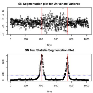
Figure 2: An example of simulated time series of model (V1). The upper panel illustrates the detection of change-points for the input time series, and the lower panel displays the segmentation of the SN test statistics using the estimated change-points. The detected change-point locations are indicated by a red vertical line and the critical value is represented by a blue horizontal line.

In addition to the summary statistics and SN based segmentation plots, the function SNSeg_estimate() provides parameter estimates within each segment that is separated by the estimated change-points. To illustrate this, we apply the following command to the same example.

SNSeg_estimate(SN_result = result1)# output$variance[1] 1.438164 5.065029 1.341965attr(,"class")[1] "SNSeg_estimate"

We can also manually specify the value of grid_size to calculate the critical value $K_{n}$ and estimate change-points. The function SNSeg_Uni() is applied to the same time series, with the only difference being that the window size $h$ is set to 102, which corresponds to grid_size_scale=0.1, instead of NULL. We further set confidence at 90%. The estimated change-points and the critical value $K_{n}$ can be obtained using the following commands:

# SNCP in the change of variance with a different grid_size and confidence levelresult2 <- SNSeg_Uni(ts, paras_to_test = "variance", confidence = 0.9,grid_size_scale = 0.05, grid_size = 102, plot_SN = FALSE,est_cp_loc = FALSE)result2$est_cp[1] 411 744result2$grid_size[1] 102result2$critical_value[1] 111.1472

Note that since grid_size is not NULL, the argument grid_size_scale = 0.05 will be ignored by the function SNSeg_Uni(). Interestingly, though we use quite different window size $h=102$, the estimated change-points are almost the same as before, which suggests the robustness of SNCP. The critical value differs from the previous example, due to the variation in the window size $h$ (or equivalently $\epsilon$). In other words,the threshold $K_{n}$ used in SNCP reflects the influence of the chosen window size $h$ (or $\epsilon$), which makes the change-point detection more robust and accurate.

Example 2: second moment change in univariate time series with a user-defined function

In addition to the built-in parameter choices, the function SNSeg_Uni() allows users to customize the input parameter using their own function. For instance, if users are interested in examining changes in the second moment, they can create a function that yields the mean square as a numeric value and designate this function to the input argument for paras_to_test. To illustrate, we consider the model (V1) from Example 1. The function SNSeg_Uni() is utilized with the default input configuration, except that we now assess the change in the second moment of the data. The specified paras_to_test, along with the execution time and the resultant estimated change-points, can be acquired using the following commands:

# define a function for paras_to_test# change in 2nd momentsecond_moment <- function(ts){result <- mean(ts^2)return(result)}start.time <- Sys.time()result.general <- SNSeg_Uni(ts, paras_to_test = second_moment, confidence = 0.9,grid_size_scale = 0.05, grid_size = NULL,plot_SN = FALSE, est_cp_loc = TRUE)end.time <- Sys.time()as.numeric(difftime(end.time,start.time)) # execution time (in minutes)result.general$est_cp # change-point estimates# Output> as.numeric(difftime(end.time,start.time)) # execution time (in minutes)[1] 22.0148> result.general$est_cp # change-point estimates[1] 412 749

As evident from the above results, SNCP detected two change-points at $\hat{k}=412,749$ when examining changes in the second moment. The estimated change-points are close to the locations of the true change-point locations, 400 and 750, respectively.

To illustrate the computational efficiency of the built-in choices of paras_to_test (i.e., "mean", "variance", etc.) another example is given to detect changes in variance but using the user-defined functional var(), which is then compared with the built-in option paras_to_test = "variance" in terms of the execution time. The comparison result can be accessed using the following commands:

start.time <- Sys.time()result1 <- SNSeg_Uni(ts, paras_to_test = "variance", confidence = 0.9,grid_size_scale = 0.05, grid_size = NULL, plot_SN = TRUE,est_cp_loc = TRUE)end.time <- Sys.time()difftime(end.time,start.time)) # built-in parameter time# user defined varianceparas_to_test <- function(ts){var(ts)}start.time <- Sys.time()result.general <- SNSeg_Uni(ts, paras_to_test = paras_to_test, confidence = 0.9,grid_size_scale = 0.05, grid_size = NULL,plot_SN = FALSE, est_cp_loc = TRUE)end.time <- Sys.time()difftime(end.time,start.time) # general functional parameter timec(result1$est_cp,result.general$est_cp)# output> difftime(end.time,start.time) # built-in parameter timeTime difference of 4.702668 secs> difftime(end.time,start.time) # general functional parameter timeTime difference of 13.39276 mins> result1$est_cp # built-in parameter estimate[1] 411 748> result.general$est_cp # general functional estimate[1] 411 748

Both methods can accurately estimate change-points, but utilizing the built-in parameter significantly reduces computation time compared to using user-defined function. The former method optimizes efficiency by leveraging the linear structure of variance calculation and is implemented via dynamic programming with the cumsum() function. In contrast, the latter method, employing a user-defined function, does not utilize the linear structure of variance (since it takes a general functional as an input which may not have a specific structure) and instead recursively calculates all subsample variances, leading to redundant calculations and increased computational time.

Example 3: multiple-parameter change in univariate time series

In addition to identifying changes in a single parameter, SNSeg_Uni() also allows for estimating change-points by simultaneously combining information across multiple parameters. This can be done by modifying the paras_to_test argument. For example, users can specify paras_to_test = c("mean", "acf", 0.6, 0.9) to simultaneously detect changes in mean, autocorrelation, 60% and 90% quantile of the input time series.

We consider the simulated univariate time series of model (MP1) in Section 4.4 of Zhao et al. (2022), where the true change-points are located at $k=333$ and 667. In particular,

$$(\mathrm{MP}1):Y_{t}=\begin{cases}X_{t},&t\in[1,333]\\ F^{-1}\left(\Phi\left(X_{t}\right)\right),&t\in[334,667]\\ X_{t},&t\in[668,1000],\end{cases}$$

where $\{X_{t}\}_{t=1}^{n}$ follows an AR(1) process with $X_{t}=0.2X_{t-1}+\sqrt{1-\rho^{2}}\epsilon_{t}$, $\epsilon_{t}$ is a sequence of i.i.d. $N(0,1)$ random variables, $\Phi(\cdot)$ denotes the CDF of $N(0,1)$, and $F(\cdot)$ denotes a mixture of a truncated normal and a generalized Pareto distribution (GPD). In particular, $F(x)=0.5F_{1}(x)+0.5F_{2}(x)$, where $F_{1}(x)=2\Phi(x),x\leq 0$ is a standard normal distribution truncated at 0 and $F_{2}(x)=1-(1+\xi(x-\mu)/\sigma)_{+}^{-1/\xi}$ is a GPD distribution with the location parameter $\mu=0$, scale parameter $\sigma=2$ and tail index $\xi=0.125$. Note that $F^{-1}(q)=\Phi^{-1}(q)$ for $q\leq 0.5$ and $F^{-1}(q)\neq\Phi^{-1}(q)$ for $q>0.5.$

To showcase the versatility of SNCP, we first detect change-points based on the 90% quantiles, where we set the grid_size_scale at $0.1$ and confidence at 0.9.

set.seed(7)require(truncnorm)require(evd)mix_GauGPD <- function(u, p, trunc_r, gpd_scale, gpd_shape) {# function for generating a mixture of truncated normal + GPDindicator <- (u < p)rv <- rep(0, length(u))rv[indicator > 0] <- qtruncnorm(u[indicator > 0] / p, a = -Inf, b = trunc_r)rv[indicator <= 0] <- qgpd((u[indicator <= 0] - p) / (1 - p), loc = trunc_r,scale = gpd_scale, shape = gpd_shape)return(rv)}# Generate model (MP1)n <- 1000cp_sets <- c(0, 333, 667, 1000)rho <- 0.2ts <- MAR(n, 1, rho) * sqrt(1 - rho ^ 2) # generate AR(1)trunc_r <- 0p <- pnorm(trunc_r)gpd_scale <- 2gpd_shape <- 0.125ts[(cp_sets[2] + 1):cp_sets[3]] <-mix_GauGPD(u = pnorm(ts[(cp_sets[2] + 1):cp_sets[3]]), p, trunc_r, gpd_scale, gpd_shape)# SNCP in the change of 90% quantileresult_q9 <- SNSeg_Uni(ts, paras_to_test = c(0.9), confidence = 0.9,grid_size_scale = 0.1, plot_SN = FALSE, est_cp_loc = FALSE)# Outputresult_q9$est_cp[1] 332 667result_q9$grid_size[1] 100result_q9$critical_value[1] 110.9993

As observed, the estimated change-points take place at $\hat{k}=332$ and 667, which are close to the locations of the true change-points. We can further use SNCP to examine if there is any change in the variance for the same time series.

# SNCP in the change of varianceresult_v <- SNSeg_Uni(ts, paras_to_test = c(’variance’), confidence = 0.9,grid_size_scale = 0.1, plot_SN = FALSE, est_cp_loc = FALSE)# Outputresult_v$est_cp[1] 329 665result_v$grid_size[1] 100result_v$critical_value[1] 110.9993

The estimated change-points in variance take place at $\hat{k}=329$ and 665, which are close to the estimated change-points in the 90% quantile. To reconcile the two sets of estimated change-points, we can further examine changes in variance the 90% quantile simultaneously using SNCP, which gives a final estimate of 331 and 667.

# SNCP in the change of variance and 90% quantileresult_q9v <- SNSeg_Uni(ts, paras_to_test = c(0.9, ’variance’), confidence = 0.9,grid_size_scale = 0.1, plot_SN = TRUE, est_cp_loc = TRUE)# Outputresult_q9v$est_cp[1] 331 667result_q9v$grid_size[1] 100result_q9v$critical_value[1] 167.4226

For practitioners, how to further identify which component(s) in “paras_to_test” changes is an interesting question. A natural strategy is as follows. For each detected change-point $\hat{\tau}$, we first construct a local window centered around it, e.g. $[\hat{\tau}-\epsilon n,\hat{\tau}+\epsilon n]$, where the local window should only contain a single change-point (with high probability). Within the local window, we then apply SNSeg_Uni() for each parameter in “paras_to_test” and test if it changes.

3.2  SNCP for Multivariate Time Series

The SN based change-point estimation for multivariate time series can be implemented via the function SNSeg_Multi(). In particular, SNSeg_Multi() allows change-point detection in multivariate means or covariance matrix of the input time series. The R code is given as:

SNSeg_Multi(ts, paras_to_test = "mean", confidence = 0.9, grid_size = NULL,grid_size_scale = 0.05, plot_SN = FALSE, est_cp_loc = TRUE)

The input arguments of confidence, grid_size, grid_size_scale and est_cp_loc are the same as those in the function SNSeg_Uni(), and the difference lies in ts, plot_SN and paras_to_test.

• ts: Input time series $\{Y_{t}=(Y_{t1},\cdots,Y_{tp})\}_{t=1}^{n}$ as a matrix, i.e., a multivariate time series represented as a matrix with $n$ rows and $p$ columns, where each column is a univariate time series. The dimension $p$ for ts should be at least 2.

• paras_to_test: A string that specifies the parameter that SNCP aims to examine. Available options of paras_to_test include:

  • "mean": The function performs change-point estimation on the mean of the multivariate time series.

  • "covariance": The function performs change-point estimation on the covariance matrix of the multivariate time series.

• plot_SN: A Boolean value that specifies whether to generate time series segmentation plot or not. SNSeg_Multi returns a plot for each individual time series if plot_SN = TRUE.

When necessary, the function SNSeg_Multi() applies the same linear interpolation rule as SNSeg_Uni() to determine the critical value for the SN test. When called, SNSeg_Multi() returns an S3 object of class SNSeg_Multi comprising the grid_size, SN_sweep_result, est_cp, confidence and critical_value, which have already been described in the context of the function SNSeg_Uni(). It also generates plots for each time series when plot_SN = TRUE. Similar to SNSeg_Uni, S3 objects of class SNSeg_Multi are also supported by print(), summary() and plot() functions.

Example 4: mean change in multivariate time series

We consider model (M2) in Section 4.2 of Zhao et al. (2022), which is generated by

$$(\mathrm{M}2):Y_{t}=\begin{cases}-3/\sqrt{5}+X_{t},&t\in[1,75],[526,575],\\ 0+X_{t},&t\in[76,375],[426,525],[576,1000],\\ 3/\sqrt{5}+X_{t},&t\in[376,425].\end{cases}$$

where $X_{t}$ is a 5-dimensional VAR(1) process with $X_{t}=0.5X_{t-1}+\epsilon_{t}$, and $\epsilon_{t}$ is a sequence of i.i.d. $N(0,\mathbf{I}_{5})$ random vectors.

The five true change-points occur at $k=75,375,425,525$ and 575. We analyze it by examining the change in multivariate means using grid_size_scale at $0.05$ and confidence at 0.9. The code implementation is as follows:

# Generate model (M2)set.seed(7)d <- 5n <- 1000cp_sets <- c(0, 75, 375, 425, 525, 575, 1000)mean_shift <- c(-3, 0, 3, 0, -3, 0) / sqrt(d)rho_sets <- 0.5sigma_cross <- list(diag(d))ts <- MAR_MTS_Covariance(n, 1, rho_sets, cp_sets = c(0, n), sigma_cross)[[1]] # generate VAR(1)no_seg <- length(cp_sets) - 1for (index in 1:no_seg) { # Mean shifttau1 <- cp_sets[index] + 1tau2 <- cp_sets[index + 1]ts[, tau1:tau2] <- ts[, tau1:tau2] + mean_shift[index]}par(mfrow=c(2,3))# SNCP in the change of multivariate meanresult_multimean <- SNSeg_Multi(ts, paras_to_test = "mean", confidence = 0.9,grid_size_scale = 0.05, plot_SN = TRUE,est_cp_loc = TRUE)# Outputresult_multimean$est_cp[1] 80 373 423 526 576result_multimean$grid_size[1] 50result_multimean$critical_value[1] 415.8649

The estimated change-points are $\hat{k}=80,373,423,526$ and 576 with a window size $h=50$ and a critical value of 415.8649. This result again closely aligns with the true change-point locations. The output of SNSeg_Multi() also allows for the use of function max_SNsweep() for plotting the segmentation of the SN test statistics. The code implementation is as follows:

SNstat_multimean <- max_SNsweep(result_multimean, plot_SN = TRUE, est_cp_loc = TRUE,critical_loc = TRUE)plot(ts[1, ], main = ’SN Segmentation Plot for the First Time Series’)abline(v = result_multimean$est_cp, col = ’red’)

Figure 3 plots the associated SN test statistics and estimated change-points. For illustration, we also plot the first time series $\{Y_{t,1}\}_{t=1}^{n}$ along with the estimated change-points.

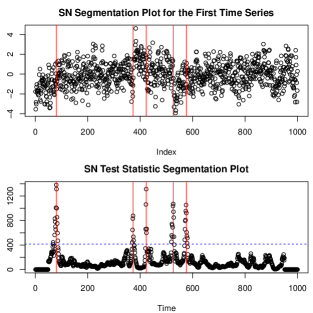
Figure 3: The segmentation of the SN test statistics using the estimated change-points. The detected change-point locations are indicated by a red vertical line and the critical value is represented by a blue horizontal line.

3.3  SNHD for High-Dimensional Time Series

The function SNSeg_HD() is specifically designed to estimate change-points in the mean functional of high-dimensional time series. The R code is given as:

SNSeg_HD(ts, confidence = 0.9, grid_size_scale = 0.05, grid_size = NULL,plot_SN = FALSE, est_cp_loc = TRUE, ts_index = c(1:5)

Its input arguments are the same as the function SNSeg_Multi() except for the followings:

• ts: The dimension of the input time series ts should be at least 10 to ensure a decent finite sample performance of the asymptotic theory.

• plot_SN: A Boolean value that specifies whether to return a plot for individual time series.

• ts_index: A positive integer or a vector of positive integers that specifies which individual time series to plot given plot_SN = TRUE. The default value is c(1:5), and under the default setting, the function will plot the first 5 time series.

When called, SNSeg_HD() returns an S3 object of class SNSeg_HD containing grid_size, SN_sweep_result, est_cp, confidence and critical_value that are similar to those described by SNSeg_Uni() and SNSeg_Multi(). It also generates a plot for the time series specified by the argument ts_index when plot_SN = TRUE. Additionally, S3 objects of class SNSeg_HD are supported by plot(), summary() and print() functions. Similar to the core function SNSeg_HD(), the plot() method incorporates the option ts_index, enabling users to visualize the desired time series.

Example 5: mean change in high-dimensional time series

We generate high-dimensional time series data based on the following simulation setting:

$$(\mathrm{HD}):Y_{t}=\mu_{i}+X_{t},~{}~{}\tau_{i-1}+1\leq t\leq\tau_{i},~{}~{}i=1,2,\cdots,6,$$

where $X_{t}$ is a sequence of i.i.d. $N(0,I_{100})$ random vectors and the five change-points are evenly located at $(\tau_{1},\tau_{2},\cdots,\tau_{5})=(100,200,\cdots,500),$ with $\tau_{0}=0$ and $\tau_{6}=600$. We set $\mu_{1}=\mathbf{0}_{100}$, $\theta_{i}=\mu_{i+1}-\mu_{i}$, $\theta_{i}=(-1)^{i}(\mathbf{1}_{5}^{\top},\mathbf{0}_{95}^{\top})^{\top}\times\sqrt{4/5}$ for $i=1,2,\cdots,5.$ We apply SNSeg_HD() to analyze this time series with grid_size_scale set at $0.05$ and confidence set at 0.9.

# Generate model (HD)set.seed(7)p <- 100n <- 600cp_sets <- c(0, 100, 200, 300, 400, 500, 600)mean_shift <- c(0, sqrt(4 / 5), 0, sqrt(4 / 5), 0, sqrt(4 / 5))ts <- matrix(rnorm(n * p, 0, 1), n, p)no_seg <- length(cp_sets) - 1for (index in 1:no_seg) { # Mean shifttau1 <- cp_sets[index] + 1tau2 <- cp_sets[index + 1]ts[tau1:tau2, 1:5] <- ts[tau1:tau2, 1:5] + mean_shift[index]}# SNHD for high-dimensional meanspar(mfrow=c(2,2))result_hd <- SNSeg_HD(ts, confidence = 0.9, grid_size_scale = 0.05,plot_SN = TRUE, est_cp_loc = TRUE,ts_index = c(1:4))# Outputresult_hd$est_cp[1]  105 203 302 397 500

Figure 4 plots the first four individual time series and the estimated change-points as requested by the argument ts_index = c(1:4). As observed in the example, SNSeg_HD() successfully detects all the change-points in this high-dimensional time series. This result demonstrates the effectiveness and feasibility of using SN algorithms for change-point detection in high-dimensional time series.

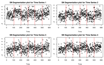
Figure 4: An example of estimating changes in high-dimensional mean for model (HD). The detected change-point locations are indicated by a red vertical line for the first 4 time series.

3.4  Generate the SN Test Statistics

As discussed in Section 2, the success of SNCP and SNHD depends on the local SN test statistic $T_{1:n}(k)$ and $T_{1,n}^{U}(k)$ for $k=1,\cdots,n$. To facilitate further analysis, the function maxSNsweep() allows the users to compute and plot these test statistics along with the identified change-points. The R code is given as:

max_SNsweep(SN_result, plot_SN = TRUE, est_cp_loc = TRUE, critical_loc = TRUE)It takes the following arguments:

• SN_result: A list generated as the output of the functions SNSeg_Uni(), SNSeg_Multi(), or SNSeg_HD().

• plot_SN: A Boolean value that specifies whether to return an SN test statistics segmentation plot.

• est_cp_loc: A Boolean value that specifies whether to plot a red vertical line for each estimated change-point.

• critical_loc: A Boolean value that specifies whether to plot a blue horizontal line for the critical value $K_{n}$ or $K_{n}^{U}$ used in the SN test.

When called, max_SNsweep() returns the maximal SN test statistic, namely $T_{1,n}(k)$ or $T_{1,n}^{U}(k)$, for each time point $k$. In addition, it can provide a segmentation plot based on these SN test statistics. Users are able to determine whether to mark the change-point locations and the critical value on the plot.

As an illustration of max_SNsweep(), suppose we apply SNSeg_Uni() to estimate change-points and save the output as result1. The following code can be used to generate the SN test statistic $T_{1:n}(k)$ for each $k=1,\cdots,n$ and in addition the segmentation plot, which is already given in the lower panel of Figure 2.

SNstat1 <- max_SNsweep(result1, plot_SN = TRUE, est_cp_loc = TRUE, critical_loc = TRUE)

As delineated in Section 3.1, 3.2 and 3.3, functions SNSeg_Uni(), SNSeg_Multi(), and SNSeg_HD() serve as the foundation for the SNSeg_estimate() function, which facilitates the computation of parameter estimates for individual segments separated by the identified change-points. When called, SNSeg_estimate() returns an S3 object of class "SNSeg_estimate" containing the parameter estimate of each segment. The R code is given as:

SNSeg_estimate(SN_result)It takes the following argument:

• SN_result: an S3 object with class "SNSeg_Uni", "SNSeg_Multi" or "SNSeg_HD". The input of SN_result must be the output from one of the functions in SNSeg_Uni(), SNSeg_Multi() and SNSeg_HD().

We refer back to Example 1 for an illustration of its use.

4  Additional Numerical Results

This section provides additional numerical results of SNSeg. In Section 4.1, we conduct a sensitivity analysis of SNSeg_Uni() across various input parameters. Section 4.2 compares with other popular change-point estimation packages. In Section 4.3. we demonstrate the usefulness of employing multiple parameters and contrasts it with detecting changes in a single parameter. We also provide brief explanations and recommendations on the selection of quantiles.

In this section, we measure the accuracy of change-point estimation by counting the difference between the number of estimated change-points and true values $\hat{m}-m_{o}$, the Hausdorff distance $d_{H}$, and adjusted Rand index (ARI). The Hausdorff distance is defined as follows. Denote the set of true change-points as $\tau_{o}$ and the set of estimated change-points as $\hat{\tau}$, we define $d_{1}(\tau_{o},\hat{\tau})=\max_{\tau_{1}\in\hat{\tau}}\min_{\tau_{2}\in\tau_{o}}|\tau_{1}-\tau_{2}|$ and $d_{2}(\tau_{o},\hat{\tau})=\max_{\tau_{1}\in\tau_{o}}\min_{\tau_{2}\in\hat{\tau}}|\tau_{1}-\tau_{2}|$, where $d_{1}(\tau_{o},\hat{\tau})$ measures the over-segmentation error of $\hat{\tau}$ and $d_{2}(\tau_{o},\hat{\tau})$ measures the under-segmentation error of $\hat{\tau}$. The Hausdorff distance is $d_{H}(\tau_{o},\hat{\tau})=\max\{d_{1}(\tau_{o},\hat{\tau}),d_{2}(\tau_{o},\hat{\tau})\}$. The ARI is originally proposed in Morey and Agresti (1984) as a measure of similarity between two different partitions of the same observations for evaluating the accuracy of clustering. Under the change-point setting, we calculate the ARI between partitions of the time series given by $\hat{\tau}$ and $\tau_{o}$. Ranging from 0 to 1, a higher ARI indicates more coherence between the two partitions by $\hat{\tau}$ and $\tau_{o}$ and thus more accurate change-point estimation. We further note that all numerical results in this section are implemented on a laptop with 1.7 GHz 12th Gen Intel Core i7 CPU and 64 GB of RAM.

4.1  Sensitivity analysis of SNCP

We first examine the performance variations resulted from choices of the trimming parameter $\epsilon$ and threshold $K_{n}$ (reflected by the confidence level $q$) when multiple change-points exist. Specifically, we generate the data according to model (SA):

$$(\mathrm{SA}):n=1200,\rho=0.5,Y_{t}=\begin{cases}0+X_{t},&t\in[1,150],[301,450],[601,750],[901,1050]\\ \delta+X_{t},&t\in[151,300],[451,600],[751,900],[1051,1200],\end{cases}$$

where $\{X_{t}\}_{t=1}^{n}$ is generated from a unit-variance AR(1) process with $X_{t}=X_{t-1}/2+\sqrt{3}\epsilon_{t}/2$, and $\{\epsilon_{t}\}$ is i.i.d. $N(0,1)$. We vary $\delta\in\{\sqrt{3},\sqrt{6}\}$ to compare the results under low and high signal-to-noise ratios.

Table 1: Sensitivity analysis of $\epsilon$ and $q$ for time series model (SA) with $\delta\in\{\sqrt{3},\sqrt{6}\}$.

					$\hat{m}-m_{o}$
$\delta$	$(q,\epsilon)$	$\leq-3$	$-2$	$-1$	$0$	$1$	$2$	$\geq 3$	ARI	$d_{1}$	$d_{2}$	$d_{H}$	time
$\sqrt{3}$	0.90, 0.05	0	1	89	882	27	1	0	0.933	1.12	2.18	2.18	1.59
	0.95, 0.05	0	26	175	788	11	0	0	0.918	1.01	3.38	3.38	1.59
	0.90, 0.08	0	33	195	772	0	0	0	0.911	0.97	3.65	3.65	0.59
	0.95, 0.08	16	85	302	597	0	0	0	0.880	0.92	5.92	5.92	0.59
	0.90, 0.10	0	4	58	938	0	0	0	0.931	1.02	1.75	1.75	0.36
	0.95, 0.10	0	24	120	856	0	0	0	0.919	0.99	2.74	2.74	0.36
	0.90, 0.12	0	4	130	866	0	0	0	0.933	0.77	2.17	2.17	0.24
	0.95, 0.12	1	14	159	826	0	0	0	0.926	0.76	2.69	2.69	0.24
	0.90, 0.15	1000	0	0	0	0	0	0	0.002	0.00	49.98	49.98	0.13
	0.95, 0.15	1000	0	0	0	0	0	0	0.001	0.00	50.01	50.01	0.13
$\sqrt{6}$	0.90, 0.05	0	0	4	964	31	1	0	0.965	0.77	0.60	0.77	1.60
	0.95, 0.05	0	0	11	968	21	0	0	0.965	0.66	0.79	0.79	1.60
	0.90, 0.08	0	0	16	984	0	0	0	0.963	0.58	0.77	0.77	0.67
	0.95, 0.08	0	2	48	950	0	0	0	0.958	0.57	1.17	1.17	0.67
	0.90, 0.10	0	0	2	998	0	0	0	0.961	0.62	0.65	0.65	0.37
	0.95, 0.10	0	0	8	992	0	0	0	0.961	0.62	0.72	0.72	0.37
	0.90, 0.12	0	0	34	966	0	0	0	0.958	0.59	0.95	0.95	0.25
	0.95, 0.12	0	0	34	966	0	0	0	0.958	0.59	0.95	0.95	0.25
	0.90, 0.15	1000	0	0	0	0	0	0	0.000	0.00	50.01	50.01	0.16
	0.95, 0.15	1000	0	0	0	0	0	0	0.000	0.00	50.01	50.01	0.16

We vary $\epsilon\in\{0.05,0.08,0.10,0.12,0.15\}$ and $q\in\{0.90,0.95\}$, and study how they affect the performance of SNCP. The numerical result over 1000 replications is summarized in Table 1 for reader’s convenience. From the table, we find that as long as the window size $\epsilon$ is smaller than the minimum spacing $\epsilon_{o}=0.125$, the performance of SNCP is quite robust and stable across the choices of $\epsilon$ and $q$. However, SNCP fails to detect changes with the window size $\epsilon=0.15>\epsilon_{o}$, highlighting the importance of selecting an appropriate value for $\epsilon$. Furthermore, we find that the execution time increases with diminishing values of $\epsilon$, while no discernible disparity in execution time is found across various thresholds.

We also briefly study the execution time of SNCP using SNSeg_Uni() across multiple model parameters including mean, variance, autocorrelation (ACF), 90% quantile, and a multi-parameter scenario with both variance and 90% quantile. For model (V1) from Example 1 and (MP1) from Example 3, Table 2 presents the averaged execution time over 100 replications of SBSeg_Uni(). The execution time of SNCP varies in the order of mean, variance, ACF, and quantile, progressing from the lowest to the highest. Notably, the multi-parameter scenario requires a longer runtime compared to the single-parameter cases.

Table 2: Execution time (in seconds) of SNCP for different parameters when applied to the models (V1) and (MP1) averaged over 100 replications.

Model	mean	variance	ACF	quantile	multi-parameter
V1	1.75	5.86	8.83	17.80	31.83
MP1	1.68	5.82	8.52	16.56	31.06

4.2  Comparison: SNCP vs BinSeg, PELT, MOSUM and ECP

We next compare SNCP with BinSeg, PELT, MOSUM and ECP in terms of the accuracy of change-point estimates, especially when data exhibits temporal dependence. BinSeg and PELT are implemented by the package changepoint (the functions cpt.mean() and cpt.var(), respectively), MOSUM utilizes the package mosum (the function mosum()), and ECP adopts the package ecp (the function e.divisive()). For SNCP, we set the trimming parameter $\epsilon=0.05$ and confidence level $q=0.9$, adhering to its default configuration. The input parameters for other methods are also chosen as default values. In particular, the default thresholds for MOSUM and ECP are based on critical values of asymptotic null distribuions under confidence level 0.95; while that for BinSeg and PELT are non-asymptotic. For the bandwidth parameter G that requires manual selection in the function mosum() for MOSUM, we let G=100. This choice aligns with the recommendation in Section 3.5 from Eichinger and Kirch (2018) that G should be half the minimal distance between two change points. In the case of model (M) below, this minimum distance is 200.

We first compare the performance of all methods under the no change-point scenario, where the time series is stationary with no change-point. We simulate a stationary univariate time series $\{Y_{t}\}_{t=1}^{n=1000}$ from a unit-variance AR(1) process $Y_{t}=\rho Y_{t-1}+\sqrt{1-\rho^{2}}\epsilon_{t}$ where $\{\epsilon_{t}\}$ is i.i.d. $N(0,1)$. We vary $\rho\in\{0,0.4,0.7\}$ to investigate the robustness of SNCP (and other methods) against false positives (i.e. type-I error) under different levels of temporal dependence.

The experiment is repeated 1000 times for each $\rho$, and the results are documented in Table 3. In general, under their respective default settings, all methods provide satisfactory type-I error control when there is no temporal dependence ($\rho=0$) whereas MOSUM and ECP are prone to produce false positives when dependence is moderate ($\rho=0.4$). Under strong temporal dependence ($\rho=0.7$), all tests exhibit high false-positive rates and SNCP is the most robust option.

Table 3: Number of change-points detected of each method when there is no change-point.

$n=1000$		$\rho=0$			$\rho=0.4$			$\rho=0.7$
$\hat{m}$	$0$	$1$	$\geq 2$	$0$	$1$	$\geq 2$	$0$	$1$	$\geq 2$
SNCP	910	82	8	884	111	5	744	210	46
BinSeg	1000	0	0	963	35	2	558	240	202
PELT	1000	0	0	943	30	27	152	66	782
MOSUM	954	43	3	292	330	378	7	16	977
ECP	952	24	24	145	72	783	0	0	1000

We further examine their power performance under model (M):

$$(\mathrm{M}):n=1000,\rho\in\{0,0.4,0.7\},Y_{t}=\begin{cases}X_{t},&t\in[1,200],[401,600],[801,1000]\\ 2+X_{t},&t\in[201,400],[601,800].\end{cases}$$

Here $\{X_{t}\}_{t=1}^{n}$ is generated from a unit-variance AR(1) process that $X_{t}=\rho X_{t-1}+\sqrt{1-\rho^{2}}\epsilon_{t}$, and $\{\epsilon_{t}\}$ is i.i.d. $N(0,1)$. The true change-points occur at 200, 400, 600 and 800. Table 4 summarizes the results over 1000 replications.

From the table, we observe that in the absence of temporal dependence ($\rho=0$), all the methods perform well, with PELT being the most effective. It should be noted that, due to the use of self-normalizer, SNCP may experience some decrease in estimation accuracy compared to other methods. When the dependence is moderate at $\rho=0.4$, SNCP demonstrates robust performance, while other competing methods tend to overestimate the number of change-points. With stronger dependence ($\rho=0.7$), SNCP exhibits the best performance based on the distribution of $\hat{m}-m_{o}$ along with $d_{H}$ and ARI, while all the other methods severely overestimate the number of change-points. In terms of the computational speed, we find that BinSeg, PELT, and MOSUM are more efficient than SNCP. Consequently, we recommend employing SNCP for change-point estimation when data exhibit moderate or strong dependence, while opting for BinSeg or PELT in cases with no or weak dependence.

Here, we only compare the results under mean shifts, and we refer the interested readers to Zhao et al. (2022) for results in other settings. Broadly speaking, our findings indicate that the SNCP exhibits greater robustness to temporal dependence compared to competing methods. However, it’s worth noting that other methods might demonstrate superior performance in instances where temporal dependence is weak. For instance, BinSeg, PELT, and MOSUM are adept at handling frequent change-points with fast computational speed.

Table 4: Performance of different methods for the time series model (M).

					$\hat{m}-m_{o}$
$\rho$	Method	$\leq-3$	$-2$	$-1$	$0$	$1$	$2$	$\geq 3$	ARI	$d_{1}$	$d_{2}$	$d_{H}$	time
$\rho=0$	SNCP	0	0	0	991	9	2	0	0.983	4.13	3.42	4.13	6.85
	BinSeg	0	0	0	961	39	0	0	0.988	3.83	3.26	3.83	0.01
	PELT	0	0	0	999	1	0	0	0.994	1.73	1.69	1.73	0.11
	MOSUM	0	0	0	993	7	0	0	0.992	3.09	2.09	3.09	0.00
	ECP	0	0	0	937	56	7	0	0.984	7.04	2.24	7.04	46.85
$\rho=0.4$	SNCP	0	0	0	972	27	1	0	0.956	8.10	5.73	8.10	5.78
	BinSeg	0	0	0	744	256	0	0	0.963	15.16	5.60	15.16	0.00
	PELT	0	0	0	862	109	29	0	0.964	14.03	3.81	14.03	0.05
	MOSUM	0	0	0	779	199	20	2	0.959	38.19	4.81	38.19	0.00
	ECP	0	0	0	170	184	217	429	0.828	87.05	4.14	87.05	54.62
$\rho=0.7$	SNCP	0	2	59	865	69	4	1	0.934	17.83	23.69	29.74	6.01
	BinSeg	0	0	0	201	799	0	0	0.930	55.11	11.30	55.11	0.00
	PELT	0	0	0	104	162	195	539	0.867	99.50	8.95	99.50	0.06
	MOSUM	0	0	0	209	414	281	96	0.909	126.3	11.06	126.3	0.00
	ECP	0	0	0	1	0	1	998	0.537	146.4	8.31	146.4	92.2

4.3  Single vs Multiple Parameters

As outlined in Section 3.1, the function SNSeg_Uni() enables users to examine changes in either a single parameter or multiple parameters. We first provide a simple example which shows that using multiple parameters may not necessarily be significantly inferior to using a single parameter, in terms of change-point estimates. This observation holds true even when the change solely stems from the single parameter. For example, we consider model (M) with $\rho=0.4$ from Section 4.2, which is solely driven by mean changes.

Table 5: Performance of SNCP based on a single parameter and multiple parameters for (M). Beginning with "SN", $\text{M, V, Q}_{20}$ represent mean, variance and 20% quantile, respectively.

					$\hat{m}-m_{o}$
Model	Method	$\leq-3$	$-2$	$-1$	$0$	$1$	$2$	$\geq 3$	ARI	$d_{1}$	$d_{2}$	$d_{H}$	time
(M)	SNM	0	0	0	972	28	0	0	0.969	8.54	6.40	8.54	1.49
	$\text{SNMQ}_{20}$	0	0	3	958	39	0	0	0.967	9.71	7.33	10.25	28.6
	SNMV	0	0	3	934	62	1	0	0.963	12.53	8.06	13.11	18.2

Table 5 summarizes the numerical results over 1000 replications. For clarity, we specify these cases using names beginning with "SN". For instance, SNM denotes SNCP for estimating changes in a single mean, $\text{SNMQ}_{20}$ represents SNCP for estimating changes in both mean and the 20% quantile, and SNMV targets the mean and variance changes simultaneously. From the table, we find that all three methods yield rather similar results, albeit mild overestimation by SNMV. This indicates that introducing additional parameters does not necessarily hinder the performance of SNCP.

We then provide another example that examining multiple parameters can outperform examining a single parameter. Specifically, we compare the performance of SNCP based on a single variance or quantile (90% or 95%) and their multi-parameter combination under the setting (MP1) from Example 3. Recall that for (MP1), the change originates from the upper quantiles and the actual change-points take place at 333 and 667. The numerical result of (MP1) over 1000 replications is taken from Table 5 of Zhao et al. (2022), and summarized in Table 6 here for readers’ convenience. Similar to Table 5, we specify the parameter settings using names beginning with "SN". For instance, SNV denotes the change in a single variance, $\text{SNQ}_{90}$ represents the change in the 90% quantile, and $\text{SNQ}_{90}\text{V}$ targets the variance and 90% quantile changes simultaneously. We observe that for (MP1), $\text{SNQ}_{90}$ and $\text{SNQ}_{95}$ performs well with a high estimation accuracy since the change of (MP1) originates from upper quantiles. By integrating changes in variance and quantiles, improvements are observed across estimation accuracy, ARI, and Hausdorff distance $d_{H}$. Notably, the combined-parameter setting $\text{SNQ}_{90,95}\text{V}$ achieves the optimal performance compared to all the other parameter configurations.

Table 6: Performance of SNCP based on the change in a single parameter and multiple parameters for (MP1). $Q_{90},Q_{95},V$ represent the change in the 90th and the 95th quantile as well as the variance respectively.

					$\hat{m}-m_{o}$
Model	Method	$\leq-3$	$-2$	$-1$	$0$	$1$	$2$	$\geq 3$	ARI	$d_{1}$	$d_{2}$	$d_{H}$
(MP1)	$\text{SNQ}_{90}$	0	10	132	805	50	3	0	0.839	3.25	7.26	7.85
	$\text{SNQ}_{95}$	0	5	100	820	73	2	0	0.868	3.16	5.70	6.62
	SNV	0	2	110	832	54	2	0	0.869	2.45	5.47	6.06
	$\text{SNQ}_{90,95}$	0	3	82	850	62	3	0	0.878	3.01	4.88	5.67
	$\text{SNQ}_{90}\text{V}$	0	0	56	869	70	5	0	0.891	3.04	3.95	4.77
	$\text{SNQ}_{95}\text{V}$	0	2	64	861	68	5	0	0.889	2.92	4.30	5.14
	$\text{SNQ}_{90,95}\text{V}$	0	2	48	882	66	2	0	0.894	2.95	3.79	4.58

Overall, our findings illustrate that employing multiple parameters does not always diminish performance of SNCP compared to using a single parameter, even when the change is primarily driven by a single parameter. Nevertheless, it is important to recognize that incorporating prior information on change types can enhance the effectiveness of SNCP.

Another aspect that is of interest is the choice of quantile for SNCP. As delineated in Section 3.1, the SNSeg_Uni() function provides users with the capability to assess variations in either a single or multiple quantiles. Particularly for practitioners, an appropriate selection of the quantile becomes pivotal when the true quantile that may change remains unknown. Table 6 for model (MP1) also offers valuable insights in this regard. Given that (MP1) experiences changes in upper quantiles, the usage of the 90% or the 95% quantile yields satisfactory results. Furthermore, the application of both 90% and 95% quantiles in combination results in an improvement compared to utilizing a single quantile.

Consequently, in cases where the specific quantile that is changing is unknown, we recommend users visually inspect their time series for signals such as peaks or troughs to assess the potential range of quantiles where changes might occur, and further employ multiple quantiles within this range for more robust change-point estimation. In other words, if one knows that the change happens in a specific range of the distribution (for example, the upper tail), we recommend he/she target several quantiles in this range (for example, targeting 90%, 95%) simultaneously, instead of picking only one quantile. In practice, it is seldom that only a particular quantile changes, while the other quantile levels near this quantile exhibit no change. Hence, testing several quantiles together can boost power and estimation accuracy to the best degree.

5  Summary

In this paper, we introduced the R package SNSeg, which provides implementations of the SN-based procedures for change-points estimation in univariate, multivariate, and high-dimensional time series. We described the main functions of the package, namely SNSeg_Uni(), SNSeg_Multi(), SNSeg_HD(), which enable the detection of change-points in a single or multiple parameter(s) of the time series. Furthermore, we presented examples demonstrating the usage of the package, including visualizing both the time series data and the segmentation plots of the SN test statistics, as well as the computation of parameter estimates within the segments that are separated by the estimated change-points.

The SNSeg package offers a comprehensive set of tools to effectively identify change-points in time series data. We hope the availability of SNSeg on CRAN can help facilitate the analysis and understanding of temporal patterns and dynamics for both researchers and practitioners.

Shubo Sun
University of Miami
Herbert Business School
Coral Gables, FL, USA
sxs3935@miami.edu

Zifeng Zhao
University of Notre Dame
Mendoza College of Business
Notre Dame, IN, USA
zifeng.zhao@nd.edu

Feiyu Jiang
Fudan University
School of Management
Shanghai, China
jiangfy@fudan.edu.cn

Xiaofeng Shao
University of Illinois at Urbana-Champaign
Department of Statistics
Champaign, IL, USA
xshao@illinois.edu

References

- Andrews (1991) D. W. Andrews. Heteroskedasticity and autocorrelation consistent covariance matrix estimation. Econometrica, pages 817–858, 1991.
- Auger and Lawrence (1989) I. E. Auger and C. E. Lawrence. Algorithms for the optimal identification of segment neighborhoods. Bulletin of mathematical biology, 51(1):39–54, 1989.
- Eichinger and Kirch (2018) B. Eichinger and C. Kirch. A mosum procedure for the estimation of multiple random change points. Bernoulli, 24(1):526–564, 2018.
- James and Matteson (2014) N. A. James and D. S. Matteson. ecp: An R package for nonparametric multiple change point analysis of multivariate data. Journal of Statistical Software, 62(7):1–25, 2014.
- Killick and Eckley (2014) R. Killick and I. A. Eckley. changepoint: An R package for changepoint analysis. Journal of Statistical Software, 58(3):1–19, 2014.
- Killick et al. (2012) R. Killick, P. Fearnhead, and I. A. Eckley. Optimal detection of changepoints with a linear computational cost. Journal of the American Statistical Association, 107(500):1590–1598, 2012.
- Meier et al. (2021) A. Meier, C. Kirch, and H. Cho. mosum: A package for moving sums in change-point analysis. Journal of Statistical Software, 97(8):1–42, 2021.
- Morey and Agresti (1984) L. C. Morey and A. Agresti. The measurement of classification agreement: An adjustment to the rand statistic for chance agreement. Educational and Psychological Measurement, 44(1):33–37, 1984.
- Newey and West (1987) W. K. Newey and K. D. West. A simple, positive semi-definite, heteroskedasticity and autocorrelationconsistent covariance matrix. Econometrica, 55:703–708, 1987.
- Ross (2015) G. J. Ross. Parametric and nonparametric sequential change detection in R: The cpm package. Journal of Statistical Software, 66(3):1–20, 2015.
- Shao (2010) X. Shao. A self-normalized approach to confidence interval construction in time series. Journal of the Royal Statistical Society: Series B, 72(3):343–366, 2010.
- Shao (2015) X. Shao. Self-normalization for time series: a review of recent developments. Journal of the American Statistical Association, 110:1797–1817, 2015.
- Shao and Zhang (2010) X. Shao and X. Zhang. Testing for change points in time series. Journal of the American Statistical Association, 105(491):1228–1240, 2010.
- Sun et al. (2023) S. Sun, Z. Zhao, F. Jiang, and X. Shao. SNSeg: Self-Normalization(SN) Based Change-Point Estimation for Time Series, 2023. URL https://CRAN.R-project.org/package=SNSeg. R package version 1.0.0.
- Wang and Zou (2023) G. Wang and C. Zou. cpss: an package for change-point detection by sample-splitting methods. Journal of Quality Technology, 55:61–74, 2023.
- Wang et al. (2022) R. Wang, C. Zhu, S. Volgushev, and X. Shao. Inference for change points in high-dimensional data via selfnormalization. The Annals of Statistics, 50(2):781–806, 2022.
- Zeileis et al. (2002) A. Zeileis, F. Leisch, K. Hornik, and C. Kleiber. strucchange: An r package for testing for structural change in linear regression models. Journal of Statistical Software, 7(2):1–38, 2002.
- Zeileis et al. (2003) A. Zeileis, C. Kleiber, W. Krämer, and K. Hornik. Testing and dating of structural changes in practice. Computational Statistics & Data Analysis, 44(1–2):109–123, 2003.
- Zhao et al. (2021) Z. Zhao, F. Jiang, and X. Shao. Segmenting time series via self-normalization. arXiv preprint https://arxiv.org/pdf/2112.05331v1.pdf, 2021.
- Zhao et al. (2022) Z. Zhao, F. Jiang, and X. Shao. Segmenting time series via self-normalisation. Journal of the Royal Statistical Society Series B: Statistical Methodology, 84(5):1699–1725, 2022.
- Zou et al. (2020) C. Zou, G. Wang, and R. Li. Consistent selection of the number of change-points via sample-splitting. Annals of Statistics, 48(1):413, 2020.