Precoder Design for User-Centric Network Massive MIMO with Matrix Manifold Optimization

Abstract

In this paper, we investigate the precoder design for user-centric network (UCN) massive multiple-input multiple-output (mMIMO) downlink with matrix manifold optimization. In UCN mMIMO systems, each user terminal (UT) is served by a subset of base stations (BSs) instead of all the BSs, facilitating the implementation of the system and lowering the dimension of the precoders to be designed. By proving that the precoder set satisfying the per-BS power constraints forms a Riemannian submanifold of a linear product manifold, we transform the constrained precoder design problem in Euclidean space to an unconstrained one on the Riemannian submanifold. Riemannian ingredients, including orthogonal projection, Riemannian gradient, retraction and vector transport, of the problem on the Riemannian submanifold are further derived, with which the Riemannian conjugate gradient (RCG) design method is proposed for solving the unconstrained problem. The proposed method avoids the inverses of large dimensional matrices, which is beneficial in practice. The complexity analyses show the high computational efficiency of RCG precoder design. Simulation results demonstrate the numerical superiority of the proposed precoder design and the high efficiency of the UCN mMIMO system.

I Introduction

With the rapid deployment of the fifth generation (5G) networks around the world, both industry and academia have embarked on the research of beyond 5G and the sixth generation (6G) communications [1]. Massive multiple-input multiple-output (mMIMO) has been one of the most essential technologies in 5G wireless communications and is believed to be one of the key enabling technologies for beyond 5G and 6G networks [2]. By grouping together antennas at the transmitter and the receiver, respectively, mMIMO can provide high spectral and energy efficiency using relatively simple processing [3]. The most popular paradigm of mMIMO system is the cellular mMIMO system, where each cell has one macro base station (BS) equipped with a large number of antennas. In each cell, the BS serves a number of user terminals (UTs) simultaneously on the same time-frequency resource. Numerous studies have validated the advantages of cellular mMIMO systems in enhancing the spectral and energy efficiency [4, 5, 6]. Nonetheless, cell-edge UTs suffer from severe performance loss in cellular mMIMO systems due to the low channel gain and the high interference from the adjacent BSs [7], which is an inherent problem in the cellular mMIMO system and difficult to deal with. Moreover, the handover at the cell edge may cause service interruption and delay during user mobility. With the increase of center frequency and decrease of cell radius in next generation wireless networks, these issues might become more severe [8].

Network mMIMO system has been proposed to enhance the performance of cell-edge UTs via coherent joint transmission [9, 10]. In the network mMIMO system, several macro BSs equipped with a large number of antennas share the data messages and channel state information (CSI) via backhaul links. Each UT in the network is served by all the BSs and seamless services are therefore guaranteed, which not only improves the performance, but also reduces the unnecessary handover and link outage probabilities [10]. Recently, a novel paradigm of mMIMO system called cell-free mMIMO is also proposed to improve the quality of service for cell-edge UTs [11]. In cell-free mMIMO systems, the large number of transmitters, referred to as access points (APs), are geographically distributed in the network and connected to a central processing unit (CPU) responsible for coherent transmission via backhaul links. Like network mMIMO system, each UT is served by all the APs in the cell-free mMIMO system and hence the notion of cell-edge disappears [12]. Compared with the network mMIMO system, the APs equipped with a much smaller number of antennas are distributed in the network much more densely in the cell-free mMIMO system. A mass of studies have borne out the superiority of the cell-free mMIMO system in boosting the performance gains, spectral efficiency, and energy efficiency compared with the cellular system [11, 12, 13]. However, the deployment of such a large number of APs in the real sites is a critical issue for the operators [14]. The geographical constraints, physical obstacles, and regulatory limitations can affect the placement and density of access points, making the wide area deployment of cell-free mMIMO system a tough task [13]. It is also difficult to mitigate from cellular systems to a cell-free system with keeping service continuity [14]. Consequently, the network mMIMO system could be considered as a more feasible and smoother evolution of the existing system, and could be indispensable for the next wireless generation networks for seamless and ubiquitous coverage and performance enhancement of the cell-edge UTs.

The user-centric rule has been considered in many existing works [15, 16], and has been introduced to the cell-free mMIMO system [17]. To be specific, each UT is served by a subset of the BSs that provide the best channel conditions under the user-centric rule, limiting the number of serving transmitters for each UT. Particularly, the set of BSs providing the service for the target UT is termed as the serving cluster of the UT, and equivalently, the set of UTs served by the target BS is addressed as the served group of the BS [17]. In general, the dynamic serving cluster construction strategy is based on either received power or largest large-scale fading [18]. In the conventional network mMIMO system, serving users with distant transmitters occupies precious power and bandwidth resources but contributes little to the performance improvement for the served UT due to the high path loss. In this regard, the network mMIMO system combined with the user-centric rule leads to the user-centric network (UCN) mMIMO system that we consider in this paper. Combining the advantages of both, the UCN mMIMO system not only eliminates the notion of cell-edge and enhances the performances of cell-edge UTs, but also facilitates the implementation of the network system and reduces the dimension of the precoding matrix to be designed compared with the conventional network mMIMO system [15].

Although the inter-cell interference can be effectively suppressed in the UCN mMIMO system, the interference in the system is still severe due to the large number of UTs in the network, making the interference management become an arduous but essential task [8]. Linear precoding can subdue interference and upsurge the achievable sum rate with low complexity and thus has been widely investigated [19, 20, 21]. However, the existing methods mostly involve the inverse of large dimensional matrices, increasing the computational complexity and aggravating the burden for implementation [22, 23]. The introduction of the UCN can effectively reduce the computational complexity, but the problem is still serious as the dimension of the matrix inversion is related to the number of transmit antennas. Even worse, higher frequency band will be explored in the future 6G wireless networks and much more antennas will be equipped at the BS side, making the problems more serious [24].

Recently, matrix manifold optimization has been widely investigated in many domains [25, 26, 27, 28] due to its ability of transforming the constrained problems in Euclidean space to the unconstrained ones on manifold. Significantly, most of Riemannian methods in manifold optimization avoid the inverses of large dimensional matrices, which is of great significance for the future wireless networks. With the combination of insights from differential geometry, optimization, and numerical analysis, matrix manifold optimization usually shows an incredible advantage in dealing with the equality constraints. Therefore, manifold optimization can provide a potentially efficient way for precoder design in UCN mMIMO systems.

In this paper, we investigate the precoder design for UCN mMIMO downlink with matrix manifold optimization, whose solution space is much lower than that of the conventional network mMIMO system. We formulate a set of constraints on the weighted sum-rate (WSR) maximization problem to limit the transmit power of each BS. By proving that the precoders satisfying the constraints are on a Riemannian submanifold, we transform the constrained optimization problem in Euclidean space to an unconstrained one on the Riemannian submanifold. Then, the Riemannian ingredients, including the orthogonal projection, Riemannian gradient, retraction and vector transport, of the Riemannian submanifold are derived. With these Riemannian ingredients, Riemannian conjugate gradient (RCG) design method is proposed for solving the unconstrained optimization problem. There is no inverse of large dimensional matrix in the RCG method. The computational complexity of the proposed method is analyzed and the acquisition of the step length involves a low computational complexity, demonstrating the high computational efficiency of the RCG method for precoder design in the UCN mMIMO system. Comprehensive comparisons are made between different systems, and the simulation results confirm the superiority of the UCN mMIMO system and the high efficiency of the RCG design method.

The rest of this paper is organized as follows. In Section II, we first clarify the system model and formulate the precoder design problem in Euclidean space. Then the problem is reformulated on the Riemannian submanifold formed by the precoders satisfying the constraints. The Riemannian ingredients of the Riemannian submanifold needed in matrix manifold optimization are derived in Section III. Section IV presents the RCG design method and the complexity analysis. Simulation results are provided in Section V to validate the superiority of the UCN mMIMO system and the RCG design method. The conclusion is drawn in Section VI.

Notations: Boldface lowercase and uppercase letters represent the column vectors and matrices, respectively. We write conjugate transpose of matrix $\mathbf{A}$ as $\mathbf{A}^{H}$ while $\mathrm{tr}\left(\mathbf{A}\right)$ and $\det\left(\mathbf{A}\right)$ denote the matrix trace and determinant of $\mathbf{A}$, respectively. $\Re\left\{\mathbf{A}\right\}$ means the real part of $\mathbf{A}$ and $\mathrm{vec}\left(\mathbf{A}\right)$ is the vector-version of the matrix $\mathbf{A}$. Let the mathematical expectation be $\mathbb{E}\left\{\cdot\right\}$. $\mathbf{I}_{M}$ denotes the $M\times M$ identity matrix, whose subscript may be omitted for brevity. $\mathbf{0}$ represents the vector or matrix whose elements are all zero. $\mathrm{diag}\left(\mathbf{a}\right)$ represents the diagonal matrix with $\mathbf{a}$ along its main diagonal and $\mathrm{diag}\left(\mathbf{A}\right)$ denotes the column vector of the main diagonal of $\mathbf{A}$. Similarly, $\mathbf{D}=\mathrm{blkdiag}\left\{\mathbf{A}_{1},\cdots,\mathbf{A}_{K}\right\}$ denotes the block diagonal matrix with $\mathbf{A}_{1},\cdots,\mathbf{A}_{K}$ on the diagonal and $\left[\mathbf{D}\right]_{i}$ denotes the $i$-th matrix on the diagonal, i.e., $\mathbf{A}_{i}$. For a block matrix $\mathbf{M}$, $\mathbf{M}_{i,j}$ or $\left(\mathbf{M}\right)_{i,j}$ denotes the $\left(i,j\right)$-th submatrix of $\mathbf{M}$. $\mathrm{card}\left(\mathcal{A}\right)$ denotes the cardinality of the set $\mathcal{A}$. $\mathcal{A}\times\mathcal{B}$ denotes the Cartesian product of the sets $\mathcal{A}$ and $\mathcal{B}$ and $\left(\mathbf{A},\mathbf{B}\right)$ is an element in $\mathcal{A}\times\mathcal{B}$ with $\mathbf{A}\in\mathcal{A}$ and $\mathbf{B}\in\mathcal{B}$. The mapping $F$ from manifold $\mathcal{M}$ to manifold $\mathcal{N}$ is $F:\mathcal{M}\rightarrow\mathcal{N}:\mathbf{X}\mapsto\mathbf{Y}$ denoted as $F(\mathbf{X})=\mathbf{Y}$. The differential of $F\left(\mathbf{X}\right)$ is represented as $\mathrm{D}F\left(\mathbf{X}\right)$ while $\mathrm{D}F\left(\mathbf{X}\right)\left[{\boldsymbol{\xi}}_{\mathbf{X}}\right]$ or $\mathrm{D}F\left[{\boldsymbol{\xi}}_{\mathbf{X}}\right]$ means the directional derivative of $F$ at $\mathbf{X}$ along the tangent vector ${\boldsymbol{\xi}}_{\mathbf{X}}$.

II System Model and Problem Formulation

In this section, we first present the signal model of the UCN mMIMO system, where each user is served by a BS subset. Then we formulate the WSR-maximization precoder design problem in Euclidean space with each BS having a power constraint and each UT having its own serving cluster. By proving that the precoder set satisfying the power constraints is on a Riemannian submanifold, we transform the constrained problem in Euclidean space to an unconstrained one on the Riemannian submanifold.

II-A System Model

Consider the downlink (DL) transmission in a UCN mMIMO system, where $U$ UTs are served by $B$ BSs. The BSs are assumed to be synchronized and linked via backhaul links, which enables coherent joint transmission. Let $\mathcal{S}_{B}=\left\{1,2,\cdots,B\right\}$ and $\mathcal{S}_{U}=\left\{1,2,\cdots,U\right\}$ denote the sets of the BSs and the UTs, respectively. Each BS has $M_{t}$ transmit antennas and each UT has $M_{r}$ receive antennas. Each UT is served by a BS subset instead of by all the BSs, which reduces the computational burden of each BS. Fig. 1 provides an illustration of this UCN mMIMO system, where only four UTs and their serving clusters are plotted for illustrative purposes. To be specific, the BSs serving UT $i$, $i\in\mathcal{S}_{U}$, constitute a subset $\mathcal{B}_{i}=\left\{i_{1},i_{2},\cdots,i_{B_{i}}\right\}$ with $\mathrm{card}\left(\mathcal{B}_{i}\right)=B_{i}$. $\mathcal{B}_{i}$ is referred to as the serving cluster of UT $i$. The set $\mathcal{B}_{i},i\in\mathcal{S}_{U},$ can be formed by selecting the BSs that provide the best channel conditions for UT $i$ [15]. Similarly, the UTs served by the $k$-th BS also constitute a subset $\mathcal{U}_{k}=\left\{k_{1},k_{2},\cdots,k_{U_{k}}\right\}$ with $\mathrm{card}\left(\mathcal{U}_{k}\right)=U_{k}$, and $\mathcal{U}_{k}$ is termed as the served group of the $k$-th BS, $k\in\mathcal{S}_{B}$. This user-centric rule allows each UT to have granted service without relying on the notion of cell.

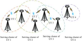
Figure 1: An illustration of the UCN mMIMO system.

Let $\mathbf{s}_{i}\in\mathbb{C}^{d_{i}}$ denote the $d_{i}$ data streams for the $i$-th UT with $\mathbb{E}\left\{\mathbf{s}_{i}\mathbf{s}_{i}^{H}\right\}=\mathbf{I}_{d_{i}},i\in\mathcal{S}_{U},$ and $\mathbb{E}\left\{\mathbf{s}_{i}\mathbf{s}_{j}^{H}\right\}=\boldsymbol{0},j\neq i,j\in\mathcal{S}_{U}$. $\mathbf{H}_{i,k}\in\mathbb{C}^{M_{r}\times M_{t}}$ is the channel matrix from the $k$-th BS to the $i$-th UT and $\mathbf{P}_{i,k}\in\mathbb{C}^{M_{t}\times d_{i}}$ is the precoding matrix designed for UT $i$ by the $k$-th BS, $k\in\mathcal{B}_{i}$. The received signal of UT $i$ can be written as

$$\mathbf{y}_{i}= \sum_{k\in\mathcal{B}_{i}}\mathbf{H}_{i,k}\mathbf{P}_{i,k}\mathbf{s}_{i}+\sum_{k\in\mathcal{B}_{i}}\sum_{j\in\mathcal{U}_{k},j\neq i}\mathbf{H}_{i,k}\mathbf{P}_{j,k}\mathbf{s}_{j}$$ (1)

$$+\sum_{\ell\notin\mathcal{B}_{i}}\sum_{j\in\mathcal{U}_{\ell}}\mathbf{H}_{i,\ell}\mathbf{P}_{j,\ell}\mathbf{s}_{j}+\mathbf{z}_{i},$$

where $\mathbf{z}_{i}$ is the independent and identically distributed (i.i.d.) complex circularly symmetric Gaussian noise vector distributed as $\mathcal{C}\mathcal{N}\left(0,\sigma_{z}^{2}\mathbf{I}_{M_{r}}\right)$. Denote

$$\mathbf{z}_{i}^{\prime} =\sum_{k\in\mathcal{B}_{i}}\sum_{j\in\mathcal{U}_{k},j\neq i}\mathbf{H}_{i,k}\mathbf{P}_{j,k}\mathbf{s}_{j}+\sum_{\ell\notin\mathcal{B}_{i}}\sum_{j\in\mathcal{U}_{\ell}}\mathbf{H}_{i,\ell}\mathbf{P}_{j,\ell}\mathbf{s}_{j}+\mathbf{z}_{i}$$ (2)

$$=\sum_{j\neq i}\sum_{\ell\in\mathcal{B}_{j}}\mathbf{H}_{i,\ell}\mathbf{P}_{j,\ell}\mathbf{s}_{j}+\mathbf{z}_{i}$$

as the inter-user interference plus noise of UT $i$, whose covariance matrix is given by

$$\mathbf{R}_{i}=\sum_{j\neq i}\Bigg{(}\sum_{\ell\in\mathcal{B}_{j}}\mathbf{H}_{i,\ell}\mathbf{P}_{j,\ell}\Bigg{)}\Bigg{(}\sum_{\ell\in\mathcal{B}_{j}}\mathbf{H}_{i,\ell}\mathbf{P}_{j,\ell}\Bigg{)}^{H}+\sigma_{z}^{2}\mathbf{I}_{M_{r}}.$$ (3)

By stacking the $\mathbf{P}_{i,k},k\in\mathcal{B}_{i}$, the precoder to be designed for UT $i$ can be defined as

$$\mathbf{P}_{i}:=\left[\mathbf{P}_{i,i_{1}}^{T},\cdots,\mathbf{P}_{i,i_{B_{i}}}^{T}\right]^{T}\in\mathbb{C}^{B_{i}M_{t}\times d_{i}}.$$ (4)

Note that the numbers of the rows and columns of the precoders for different users may be different. Let $\mathbf{H}_{i}:=\left[\mathbf{H}_{i,1},\mathbf{H}_{i,2},\cdots,\mathbf{H}_{i,B}\right]\in\mathbb{C}^{M_{r}\times BM_{t}}$ denote the stacked channel matrix of UT $i$. Further, let $\mathbf{W}_{i}\in\mathbb{R}^{BM_{t}\times B_{i}M_{t}},i\in\mathcal{S}_{U},$ be a block matrix composed of $B\times B_{i}$ submatrices, where $\left(\mathbf{W}_{i}\right)_{i_{n},n}=\mathbf{I}_{M_{t}}$ and other submatrices are $\boldsymbol{0}_{M_{t}}$. Then, (1), (2) and (3) can be rewritten as

$$\mathbf{y}_{i} =\mathbf{H}_{i}\mathbf{W}_{i}\mathbf{P}_{i}\mathbf{s}_{i}+\mathbf{H}_{i}\sum_{j\in\mathcal{S}_{U},j\neq i}\mathbf{W}_{j}\mathbf{P}_{j}\mathbf{s}_{j}+\mathbf{z}_{i},$$ (5)

$$\mathbf{z}_{i}^{\prime} =\mathbf{H}_{i}\sum_{j\in\mathcal{S}_{U},j\neq i}\mathbf{W}_{j}\mathbf{P}_{j}\mathbf{s}_{j}+\mathbf{z}_{i},$$ (6)

$$\mathbf{R}_{i} =\mathbf{H}_{i}\sum_{j\in\mathcal{S}_{U},j\neq i}\mathbf{W}_{j}\mathbf{P}_{j}\mathbf{P}_{j}^{H}\mathbf{W}_{j}^{H}\mathbf{H}_{i}^{H}+\sigma_{z}^{2}\mathbf{I}_{M_{r}}.$$ (7)

Remark 1.

If $B_{i}=B,\forall i\in\mathcal{S}_{U},$ the UCN mMIMO system is equivalent to the conventional network mMIMO system [9], where the UTs are served by all the BSs. If $B_{i}=1,\forall i\in\mathcal{S}_{U},$ the system is reduced to the cellular system [29], where each UT is served by only one BS and the signals from other BSs are treated as inter-cell interference.

II-B Problem Formulation in Euclidean Space

In this subsection, we formulate the WSR maximization precoder design problem for UCN mMIMO DL transmission in Euclidean space. For simplicity, we assume that the perfect CSI of the effective channel $\mathbf{H}_{i,k}\mathbf{P}_{i,k},\forall k\in\mathcal{B}_{i},$ is available for the $i$-th UT via DL training. In the worst case, $\mathbf{z}_{i}^{\prime}$ can be treated as an equivalent Gaussian noise with the covariance matrix $\mathbf{R}_{i}$, which is assumed to be known by UT $i$. Under these assumptions, the rate of UT $i$ can be expressed as

$$\enspace\mathcal{R}_{i} =\log\det\left(\mathbf{R}_{i}+\mathbf{H}_{i}\mathbf{W}_{i}\mathbf{P}_{i}\mathbf{P}_{i}^{H}\mathbf{W}_{i}^{H}\mathbf{H}_{i}^{H}\right)-\log\det\left(\mathbf{R}_{i}\right).$$ (8)

Assuming the transmit power of the $k$-th BS is $P_{k},k\in\mathcal{S}_{B}$, and these constraints are represented by $F\left(\mathbf{P}_{1},\cdots,\mathbf{P}_{U}\right)=\boldsymbol{0}$. The WSR-maximization precoder design problem can be formulated as

$$\mathop{\arg\min}\limits_{\mathbf{P}_{1},\cdots,\mathbf{P}_{U}} f\left(\mathbf{P}_{1},\cdots,\mathbf{P}_{U}\right)$$ (9)

$$\mathrm{s.}\mathrm{t.}\ F \left(\mathbf{P}_{1},\cdots,\mathbf{P}_{U}\right)=\boldsymbol{0},$$

where $f\left(\mathbf{P}_{1},\cdots,\mathbf{P}_{U}\right)=-\sum_{i\in\mathcal{S}_{U}}w_{i}\mathcal{R}_{i}$ is the objective function with $w_{i}$ being the weighted factor of UT $i$. The constraint $F\left(\mathbf{P}_{1},\cdots,\mathbf{P}_{U}\right)=\boldsymbol{0}_{B}$ can be expressed as

$$F\left(\mathbf{P}_{1},\cdots,\mathbf{P}_{U}\right)=$$ (10)

$$\sum_{i\in\mathcal{U}_{k}}\mathrm{tr}\left(\mathbf{P}_{i}^{H}\mathbf{W}_{i}^{H}\mathbf{Q}_{k}\mathbf{W}_{i}\mathbf{P}_{i}\right)-P_{k}=0,k\in\mathcal{S}_{B},$$

where $\mathbf{Q}_{k}=\mathrm{blkdiag}\left\{\mathbf{Q}_{k,1},\cdots,\mathbf{Q}_{k,B}\right\}\in\mathbb{C}^{BM_{t}\times BM_{t}}$ is a block diagonal matrix with $\mathbf{Q}_{k,k}=\mathbf{I}_{M_{t}}$ and $\mathbf{Q}_{k,\ell}=\boldsymbol{0}_{M_{t}\times M_{t}},\ell\neq k,k\in\mathcal{S}_{B}$.

II-C Problem Reformulation on Riemannian Submanifold

For a manifold $\mathcal{M}$, a smooth mapping $\gamma:\mathbb{R}\rightarrow\mathcal{M}:t\mapsto\gamma(t)$ is termed as a curve in $\mathcal{M}$. Let $\mathbf{X}$ denote a point on $\mathcal{M}$ and $\mathcal{F}_{\mathbf{X}}(\mathcal{M})$ denote the set of smooth real-valued functions defined on a neighborhood of $\mathbf{X}$. A tangent vector ${\boldsymbol{\xi}}_{\mathbf{X}}$ to manifold $\mathcal{M}$ at $\mathbf{X}$ is a mapping from $\mathcal{F}_{\mathbf{X}}(\mathcal{M})$ to $\mathbb{R}$ such that there exists a curve $\gamma$ on $\mathcal{M}$ with $\gamma(0)=\mathbf{X}$, satisfying ${\boldsymbol{\xi}}_{\mathbf{X}}f=\left.\frac{\mathrm{d}(f(\gamma(t)))}{\mathrm{d}t}\right|_{t=0}$ for all $f\in\mathcal{F}_{\mathbf{X}}(\mathcal{M})$. Such a curve $\gamma$ is said to realize the tangent vector ${\boldsymbol{\xi}}_{\mathbf{X}}$. The set of all the tangent vectors to $\mathcal{M}$ at $\mathbf{X}$ forms a unique and linear tangent space, denoted by $T_{\mathbf{X}}\mathcal{M}$. Particularly, every vector space $\mathcal{E}$ forms a linear manifold naturally, whose tangent space is given by $T_{\mathbf{X}}\mathcal{E}=\mathcal{E}$.

Besides, we can define the length of a tangent vector in $T_{\mathbf{X}}\mathcal{N}$ by endowing the tangent space with an inner product $g_{\mathbf{X}}^{\mathcal{N}}\left(\cdot\right)$. Note that the subscript $\mathbf{X}$ and the superscript $\mathcal{N}$ in $g_{\mathbf{X}}^{\mathcal{N}}\left(\cdot\right)$ are used to distinguish the inner product of different points on different manifolds for clarity. $g_{\mathbf{X}}^{\mathcal{N}}\left(\cdot\right)$ is called Riemannian metric if it varies smoothly and the manifold is called Riemannian manifold.

The product manifold is the Cartesian product of several manifolds. Let $\mathcal{M}_{1}$ and $\mathcal{M}_{2}$ denote two manifolds with $\mathbf{X}_{1}\in\mathcal{M}_{1}$ and $\mathbf{X}_{2}\in\mathcal{M}_{2}$, and

$$\mathcal{M}\triangleq\mathcal{M}_{1}\times\mathcal{M}_{2}$$ (11)

is called the product manifold of manifold $\mathcal{M}_{1}$ and $\mathcal{M}_{2}$ with $\mathbf{X}\triangleq\mathbf{X}_{1}\times\mathbf{X}_{2}\in\mathcal{M}$. The tangent space of the product manifold $\mathcal{M}$ is defined as

$$T_{\mathbf{X}}\mathcal{M}=T_{\mathbf{X}_{1}}\mathcal{M}_{1}\times T_{\mathbf{X}_{2}}\mathcal{M}_{2},$$ (12)

which is endowed with the inner product

$$g_{\mathbf{X}}^{\mathcal{M}}\left({\boldsymbol{\xi}}_{\mathbf{X}},{\boldsymbol{\zeta}}_{\mathbf{X}}\right)=g_{\mathbf{X}_{1}}^{\mathcal{M}_{1}}\left({\boldsymbol{\xi}}_{\mathbf{X}_{1}},{\boldsymbol{\zeta}}_{\mathbf{X}_{1}}\right)+g_{\mathbf{X}_{2}}^{\mathcal{M}_{2}}\left({\boldsymbol{\xi}}_{\mathbf{X}_{2}},{\boldsymbol{\zeta}}_{\mathbf{X}_{2}}\right).$$ (13)

From the point of view of matrix manifold, the complex vector space $\mathbb{C}^{M\times N}$ forms a linear manifold naturally. So the precoding matrix $\mathbf{P}_{i,k},k\in\mathcal{B}_{i},$ is on the manifold $\mathcal{N}_{i,k}=\mathbb{C}^{M_{t}\times d_{i}}$, whose tangent space $T_{\mathbf{P}_{i,1}}\mathcal{N}_{i,k}$ is still $\mathbb{C}^{M_{t}\times d_{i}}$ equipped with the Riemannian metric

$$g_{\mathbf{P}_{i,k}}^{\mathcal{N}_{i,k}}\left({\boldsymbol{\xi}}_{\mathbf{P}_{i,k}},{\boldsymbol{\zeta}}_{\mathbf{P}_{i,k}}\right)=\Re\left\{\mathrm{tr}\left({\boldsymbol{\zeta}}_{\mathbf{P}_{i,k}}^{H}{\boldsymbol{\xi}}_{\mathbf{P}_{i,k}}\right)\right\},$$ (14)

where ${\boldsymbol{\xi}}_{\mathbf{P}_{i,k}}$ and ${\boldsymbol{\zeta}}_{\mathbf{P}_{i,k}}$ are two tangent vectors in $T_{\mathbf{P}_{i,k}}\mathcal{N}_{i,k}$. From (11), $\mathbf{P}_{i}$ defined in (4) can be viewed as a point on a product manifold composed of $B_{i}$ manifolds defined as

$$\mathcal{N}_{i}:=\mathcal{N}_{i,1}\times\mathcal{N}_{i,2}\times\cdots\times\mathcal{N}_{i,B_{i}},i\in\mathcal{S}_{U},$$ (15)

which is equivalent to the complex vector space $\mathbb{C}^{B_{i}M_{t}\times d_{i}}$. From (12), the tangent space of $\mathcal{N}_{i}$ is given by

$$T_{\mathbf{P}_{i}}\mathcal{N}_{i}:=T_{\mathbf{P}_{i,1}}\mathcal{N}_{i,1}\times T_{\mathbf{P}_{i,2}}\mathcal{N}_{i,2}\times\cdots\times T_{\mathbf{P}_{i,B_{i}}}\mathcal{N}_{i,B_{i}},$$ (16)

whose product Riemannian metric can be defined as

$$g_{\mathbf{P}_{i}}^{\mathcal{N}_{i}}\left({\boldsymbol{\xi}}_{\mathbf{P}_{i}},{\boldsymbol{\zeta}}_{\mathbf{P}_{i}}\right)=\sum_{k\in\mathcal{B}_{i}}\Re\left\{\mathrm{tr}\left({\boldsymbol{\zeta}}_{\mathbf{P}_{i,k}}^{H}{\boldsymbol{\xi}}_{\mathbf{P}_{i,k}}\right)\right\}.$$ (17)

${\boldsymbol{\xi}}_{\mathbf{P}_{i}}=\left({\boldsymbol{\xi}}_{\mathbf{P}_{i,1}}^{H},\cdots,{\boldsymbol{\xi}}_{\mathbf{P}_{i,B}}^{H}\right)^{H}$ and ${\boldsymbol{\zeta}}_{\mathbf{P}_{i}}=\left({\boldsymbol{\zeta}}_{\mathbf{P}_{i,1}}^{H},\cdots,{\boldsymbol{\zeta}}_{\mathbf{P}_{i,B}}^{H}\right)^{H}$ are two tangent vectors in $T_{\mathbf{P}_{i}}\mathcal{N}_{i}$. Further, $\mathbf{P}:=\left(\mathbf{P}_{1},\mathbf{P}_{2},\cdots,\mathbf{P}_{U}\right)$ is on a product manifold defined as

$$\mathcal{N}:=\mathcal{N}_{1}\times\mathcal{N}_{2}\times\cdots\times\mathcal{N}_{U}.$$ (18)

The tangent space of $\mathcal{N}$ is given by

$$T_{\mathbf{P}}\mathcal{N}:=T_{\mathbf{P}_{1}}\mathcal{N}_{1}\times T_{\mathbf{P}_{2}}\mathcal{N}_{2}\times\cdots\times T_{\mathbf{P}_{U}}\mathcal{N}_{U},$$ (19)

with the Riemannian metric

$$g_{\mathbf{P}}^{\mathcal{N}}\left({\boldsymbol{\xi}}_{\mathbf{P}},{\boldsymbol{\zeta}}_{\mathbf{P}}\right)=\sum_{i\in\mathcal{S}_{U}}g_{\mathbf{P}_{i}}^{\mathcal{N}_{i}}\left({\boldsymbol{\xi}}_{\mathbf{P}_{i}},{\boldsymbol{\zeta}}_{\mathbf{P}_{i}}\right),$$ (20)

where ${\boldsymbol{\xi}}_{\mathbf{P}}=\left({\boldsymbol{\xi}}_{\mathbf{P}_{1}},\cdots,{\boldsymbol{\xi}}_{\mathbf{P}_{U}}\right)$ and ${\boldsymbol{\zeta}}_{\mathbf{P}}=\left({\boldsymbol{\zeta}}_{\mathbf{P}_{1}},\cdots,{\boldsymbol{\zeta}}_{\mathbf{P}_{U}}\right)$ are two tangent vectors in $T_{\mathbf{P}}\mathcal{N}$. With the Riemannian metric (20), $\mathcal{N}$ is a Riemannian product manifold. Let

$$\mathcal{M}:=\left\{\mathbf{P}\in\mathcal{N}\mid F\left(\mathbf{P}\right)=\boldsymbol{0}_{B}\right\}$$ (21)

denote the set of the precoders satisfying (10). Then, we have the following theorem.

Theorem 1.

$\mathcal{M}$ defined in (21) forms a Riemannian submanifold of $\mathcal{N}$ with the Riemannian metric

$$g_{\mathbf{P}}^{\mathcal{M}}\left({\boldsymbol{\xi}}_{\mathbf{P}},{\boldsymbol{\zeta}}_{\mathbf{P}}\right)=g_{\mathbf{P}}^{\mathcal{N}}\left({\boldsymbol{\xi}}_{\mathbf{P}},{\boldsymbol{\zeta}}_{\mathbf{P}}\right),{\boldsymbol{\xi}}_{\mathbf{P}},{\boldsymbol{\zeta}}_{\mathbf{P}}\in T_{\mathbf{P}}\mathcal{M}.$$ (22)

Proof.

See the proof in Appendix A. ∎

It is worth emphasizing that that $\mathbf{P}\in\mathcal{M}$ satisfying $F\left(\mathbf{P}\right)=\boldsymbol{0}_{B}$ is still on $\mathcal{N}$. So ${\boldsymbol{\xi}}_{\mathbf{P}}$ and ${\boldsymbol{\zeta}}_{\mathbf{P}}$ on the right hand side of (22) are viewed as elements in $T_{\mathbf{P}}\mathcal{N}$. From Theorem 1, we can reformulate the constrained problem (9) as an unconstrained one on $\mathcal{M}$ as

$$\mathop{\arg\min}\limits_{\mathbf{P}\in\mathcal{M}}f\left(\mathbf{P}\right).$$ (23)

III Riemannian Ingredients for Precoder Design

In this section, we derive all the Riemannian ingredients needed for solving (23) in manifold optimization, including orthogonal projection, Riemannian gradient, retraction and vector transport.

III-A Orthogonal Projection

With the Riemannian metric $g_{\mathbf{P}}^{\mathcal{N}}\left(\cdot\right)$, the tangent space $T_{\mathbf{P}}\mathcal{N}$ at $\mathbf{P}\in\mathcal{N}$ defined in (19) can be decomposed into two orthogonal subspaces as

$$T_{\mathbf{P}}\mathcal{N}=T_{\mathbf{P}}\mathcal{M}\oplus N_{\mathbf{P}}\mathcal{M},$$ (24)

where $T_{\mathbf{P}}\mathcal{M}$ and $N_{\mathbf{P}}\mathcal{M}$ are the tangent space and the normal space of $\mathcal{M}$ at $\mathbf{P}\in\mathcal{M}$, respectively. For geometric understanding, Fig. 2 is a simple illustration.

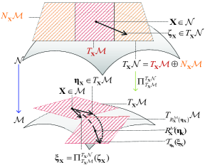
Figure 2: Geometric interpretation of orthogonal projection, retraction and vector transport.

From (10) and (21), it is easy to verify that $\mathcal{M}$ is defined as a level set of a constant-rank function $F$ [30]. In this case, $T_{\mathbf{P}}{\mathcal{M}}$ is the kernel of the differential of $F$ and a subspace of $T_{\mathbf{P}}{\mathcal{N}}$ defined as [30]

$$T_{\mathbf{P}}\mathcal{M}=\mathrm{ker}\left(\mathrm{D}F\left(\mathbf{P}\right)\right).$$ (25)

Recall that $F:\mathcal{N}\rightarrow\mathbb{R}^{B}$ defined in (10) is a smooth mapping from manifold $\mathcal{N}$ to manifold $\overline{\mathcal{M}}$, where $\mathcal{N}$ and $\overline{\mathcal{M}}$ are the manifolds formed by the vector space $\mathbb{C}^{BM_{t}\times\sum_{i=1}^{U}d_{i}}$ and $\mathbb{R}^{B}$, respectively. $\mathrm{D}F\left(\mathbf{P}\right)\left[\cdot\right]$ is thus a linear mapping from $T_{\mathbf{P}}\mathcal{N}$ to $T_{\mathbf{Y}}\overline{\mathcal{M}}$, where $\mathbf{Y}=F\left(\mathbf{P}\right)=\boldsymbol{0}_{B}$ is a point on $\overline{\mathcal{M}}$. Hence, ${\boldsymbol{\xi}}_{\mathbf{Y}}=\mathrm{D}F\left(\mathbf{P}\right)\left[{\boldsymbol{\xi}}_{\mathbf{P}}\right]$ is a tangent vector to $\overline{\mathcal{M}}$ at $\mathbf{Y}$, i.e., an element in $T_{\mathbf{Y}}\overline{\mathcal{M}}$. In particular, as $\mathcal{N}=\mathbb{C}^{BM_{t}\times\sum_{i\in\mathcal{S}_{U}}d_{i}}$ and $\overline{\mathcal{M}}=\mathbb{R}^{B}$ are both linear manifolds, $\mathrm{D}F\left(\mathbf{P}\right)$ will be reduced to the classical directional derivative

$$\mathrm{D}F\left(\mathbf{P}\right)\left[\boldsymbol{{\boldsymbol{\xi}}}_{\mathbf{P}}\right]=\lim_{t\rightarrow 0}\frac{F\left(\mathbf{P}+t\boldsymbol{{\boldsymbol{\xi}}}_{\mathbf{P}}\right)-F\left(\mathbf{P}\right)}{t}.$$ (26)

From (25) and (26), $T_{\mathbf{P}}\mathcal{M}$ is given by

$$T_{\mathbf{P}}\mathcal{M}=\Big{\{}{\boldsymbol{\xi}}_{\mathbf{P}}\in T_{\mathbf{P}}\mathcal{N}\mid\sum_{i\in\mathcal{U}_{k}}\mathrm{tr}\Big{(}{\boldsymbol{\xi}}_{\mathbf{P}_{i}}^{H}\mathbf{W}_{i}^{H}\mathbf{Q}_{k}\mathbf{W}_{i}\mathbf{P}_{i}$$ (27)

$$+\mathbf{P}_{i}^{H}\mathbf{W}_{i}^{H}\mathbf{Q}_{k}\mathbf{W}_{i}{\boldsymbol{\xi}}_{\mathbf{P}_{i}}\Big{)}=0,k\in\mathcal{S}_{B}\Big{\}}.$$

To obtain the elements in $T_{\mathbf{P}}{\mathcal{M}}$, we can obtain the corresponding elements in $T_{\mathbf{P}}{\mathcal{N}}$ first and turn to the orthogonal projection. The normal space $N_{\mathbf{P}}\mathcal{M}$ is the orthogonal complement of $T_{\mathbf{P}}\mathcal{M}$ and thus can be expressed as

$$N_{\mathbf{P}}\mathcal{M}= \Big{\{}{\boldsymbol{\zeta}}_{\mathbf{P}}\in T_{\mathbf{P}}\mathcal{N}\mid g_{\mathbf{P}}^{\mathcal{N}}\left({\boldsymbol{\xi}}_{\mathbf{P}},{\boldsymbol{\zeta}}_{\mathbf{P}}\right)=0,\forall{\boldsymbol{\xi}}_{\mathbf{P}}\in T_{\mathbf{P}}\mathcal{M}\Big{\}}$$ (28)

$$= \Big{\{}\Big{(}\sum_{\ell\in\mathcal{B}_{1}}\mu_{\ell}\mathbf{W}_{1}^{H}\mathbf{Q}_{\ell}\mathbf{W}_{1}\mathbf{P}_{1},\cdots,$$

$$\sum_{\ell\in\mathcal{B}_{U}}\mu_{\ell}\mathbf{W}_{U}^{H}\mathbf{Q}_{\ell}\mathbf{W}_{U}\mathbf{P}_{U}\Big{)}\mid\mu_{\ell}\in\mathbb{R}\Big{\}}.$$

With (24), any ${\boldsymbol{\xi}}_{\mathbf{P}}\in T_{\mathbf{P}}\mathcal{N}$ can be decomposed into two orthogonal tangent vectors as

$${\boldsymbol{\xi}}_{\mathbf{P}}={\boldsymbol{\Pi}}^{T_{\mathbf{P}}\mathcal{N}}_{T_{\mathbf{P}}\mathcal{M}}\left({\boldsymbol{\xi}}_{\mathbf{P}}\right)+{\boldsymbol{\Pi}}^{T_{\mathbf{P}}\mathcal{N}}_{N_{\mathbf{P}}\mathcal{M}}\left({\boldsymbol{\xi}}_{\mathbf{P}}\right),$$ (29)

where ${\boldsymbol{\Pi}}^{T_{\mathbf{P}}\mathcal{N}}_{T_{\mathbf{P}}\mathcal{M}}\left({\boldsymbol{\xi}}_{\mathbf{P}}\right)$ and ${\boldsymbol{\Pi}}^{T_{\mathbf{P}}\mathcal{N}}_{N_{\mathbf{P}}\mathcal{M}}\left({\boldsymbol{\xi}}_{\mathbf{P}}\right)$ represent the orthogonal projections of ${\boldsymbol{\xi}}_{\mathbf{P}}$ onto $T_{\mathbf{P}}\mathcal{M}$ and $N_{\mathbf{P}}\mathcal{M}$, respectively.

Lemma 1.

For any ${\boldsymbol{\xi}}_{\mathbf{P}}\in T_{\mathbf{P}}\mathcal{N}$, the orthogonal projection ${\boldsymbol{\Pi}}^{T_{\mathbf{P}}\mathcal{N}}_{T_{\mathbf{P}}\mathcal{M}}\left({\boldsymbol{\xi}}_{\mathbf{P}}\right)$ is given by

$${\boldsymbol{\Pi}}^{T_{\mathbf{P}}\mathcal{N}}_{T_{\mathbf{P}}\mathcal{M}}\left({\boldsymbol{\xi}}_{\mathbf{P}}\right)=\Big{(} {\boldsymbol{\xi}}_{\mathbf{P}_{1}}-\sum_{\ell\in\mathcal{B}_{1}}\mu_{\ell}\mathbf{W}_{1}^{H}\mathbf{Q}_{\ell}\mathbf{W}_{1}\mathbf{P}_{1},\cdots,$$ (30)

$${\boldsymbol{\xi}}_{\mathbf{P}_{U}}-\sum_{\ell\in\mathcal{B}_{U}}\mu_{\ell}\mathbf{W}_{U}^{H}\mathbf{Q}_{\ell}\mathbf{W}_{U}\mathbf{P}_{U}\Big{)},$$

where

$$\mu_{\ell}=\frac{1}{P_{\ell}}\sum_{i\in\mathcal{U}_{\ell}}\Re\left\{\mathrm{tr}\left(\mathbf{P}_{i}^{H}\mathbf{W}_{i}^{H}\mathbf{Q}_{\ell}\mathbf{W}_{i}{\boldsymbol{\xi}}_{\mathbf{P}_{i}}\right)\right\}.$$ (31)

Proof.

See the proof in Appendix B. ∎

III-B Riemannian Gradient

The set of all tangent vectors to $\mathcal{M}$ is called tangent bundle denoted by $T\mathcal{M}$, which itself is a smooth manifold. A vector field ${\boldsymbol{\xi}}$ on manifold $\mathcal{M}$ is a smooth mapping from $\mathcal{M}$ to $T\mathcal{M}$ that assigns to each point $\mathbf{P}\in\mathcal{M}$ a tangent vector ${\boldsymbol{\xi}}_{\mathbf{P}}\in T_{\mathbf{P}}\mathcal{M}$. Denote $\mathrm{grad}_{\mathcal{M}}f$ as the vector field of the Riemannian gradient. For the smooth real-valued function $f$ on Riemannian submanifold $\mathcal{M}$, the Riemannian gradient of $f$ at $\mathbf{P}$, denoted by $\mathrm{grad}_{\mathcal{M}}f(\mathbf{P})$, is defined as the unique element in $T_{\mathbf{P}}{\mathcal{M}}$ that satisfies

$$g_{\mathbf{P}}^{\mathcal{M}}\left(\mathrm{grad}_{\mathcal{M}}f(\mathbf{P}),\boldsymbol{{\boldsymbol{\xi}}}_{\mathbf{P}}\right)=\mathrm{D}f\left(\mathbf{P}\right)\left[\boldsymbol{{\boldsymbol{\xi}}}_{\mathbf{P}}\right],\forall{\boldsymbol{\xi}}_{\mathbf{P}}\in T_{\mathbf{P}}\mathcal{M}.$$ (32)

Note that, since $\mathrm{grad}_{\mathcal{M}}f(\mathbf{P})\in T_{\mathbf{P}}{\mathcal{M}}$, we can derive the Riemannian gradient $\mathrm{grad}_{\mathcal{M}}f\left(\mathbf{P}\right)$ in $T_{\mathbf{P}}\mathcal{M}$ by projecting the Riemannian gradient $\mathrm{grad}_{\mathcal{N}}f\left(\mathbf{P}\right)$ in $T_{\mathbf{P}}\mathcal{N}$ onto $T_{\mathbf{P}}\mathcal{M}$, which will play a significant role in obtaining the search direction in optimization. Denoting

$$\mathbf{C}_{i}=\left(\mathbf{I}_{d_{i}}+\mathbf{P}_{i}^{H}\mathbf{W}_{i}^{H}\mathbf{H}_{i}^{H}\mathbf{R}_{i}^{-1}\mathbf{H}_{i}\mathbf{W}_{i}\mathbf{P}_{i}\right)^{-1},$$ (33)

we have the following theorem.

Theorem 2.

The Euclidean gradient of $f\left(\mathbf{P}\right)$ is given by

$$\mathrm{grad}_{\mathcal{N}}f\left(\mathbf{P}\right)=\left(\mathrm{grad}_{\mathcal{N}_{1}}f\left(\mathbf{P}_{1}\right),\cdots,\mathrm{grad}_{\mathcal{N}_{U}}f\left(\mathbf{P}_{U}\right)\right),$$ (34)

where

$$\mathrm{grad}_{\mathcal{N}_{i}} f\left(\mathbf{P}_{i}\right)=$$ (35)

$$\left(\mathrm{grad}_{\mathcal{N}_{i,1}}f\left(\mathbf{P}_{i,1}\right)^{T},\cdots,\mathrm{grad}_{\mathcal{N}_{i,B}}f\left(\mathbf{P}_{i,B}\right)^{T}\right)^{T}.$$

To be specific,

$$\mathrm{grad}_{\mathcal{N}_{i,k}}f\left(\mathbf{P}_{i,k}\right)=-2\big{(}w_{i}\mathbf{H}_{i,k}^{H}\mathbf{R}_{i}^{-1}\mathbf{H}_{i}\mathbf{W}_{i}\mathbf{P}_{i}\mathbf{C}_{i}$$ (36)

$$-\sum_{j\neq i}^{U}w_{j}\mathbf{H}_{j,k}^{H}\mathbf{R}_{j}^{-1}\mathbf{H}_{j}\mathbf{W}_{j}\mathbf{P}_{j}\mathbf{C}_{j}\mathbf{P}_{j}^{H}\mathbf{W}_{j}^{H}\mathbf{H}_{j}^{H}\mathbf{R}_{j}^{-1}\mathbf{H}_{j}\mathbf{W}_{i}\mathbf{P}_{i}\big{)}$$

in $T_{\mathbf{P}_{i,k}}\mathcal{N}_{i,k}=\mathbb{C}^{M_{t}\times d_{i}}$ is the Euclidean gradient of UT $i$ served by the $k$-th BS for $k\in\mathcal{B}_{i},i\in\mathcal{S}_{U}$. The Riemannian gradient of $f\left(\mathbf{P}\right)$ in $T_{\mathbf{P}}\mathcal{M}$ is given by

$$\mathrm{grad}_{\mathcal{M}} f\left(\mathbf{P}\right)=$$ (37)

$$\Big{(}\mathrm{grad}_{\mathcal{N}_{1}}f\left(\mathbf{P}_{1}\right)-\sum_{k\in\mathcal{B}_{1}}\lambda_{k}\mathbf{W}_{1}^{H}\mathbf{Q}_{k}\mathbf{W}_{1}\mathbf{P}_{1},\cdots,$$

$$\mathrm{grad}_{\mathcal{N}_{U}}f\left(\mathbf{P}_{U}\right)-\sum_{k\in\mathcal{B}_{U}}\lambda_{k}\mathbf{W}_{U}^{H}\mathbf{Q}_{k}\mathbf{W}_{U}\mathbf{P}_{U}\Big{)},$$

where

$$\lambda_{k}=\frac{1}{P_{k}}\sum_{i\in\mathcal{U}_{k}}\Re\Big{\{}\mathrm{tr}\left(\mathbf{P}_{i}^{H}\mathbf{W}_{i}^{H}\mathbf{Q}_{k}\mathbf{W}_{i}\mathrm{grad}_{\mathcal{N}_{i}}f\left(\mathbf{P}_{i}\right)\right)\Big{\}}.$$ (38)

Proof.

See the proof in Appendix C. ∎

It is worth noting that only $\mathrm{grad}_{\mathcal{N}_{i,k}}f\left(\mathbf{P}_{i,k}\right),k\in\mathcal{B}_{i},$ are computed, which will decrease the computational complexity of $\mathrm{grad}_{\mathcal{M}}f\left(\mathbf{P}\right)$ compared with the conventional network systems.

III-C Retraction

For a nonlinear manifold, the notion of moving along the tangent vector while remaining on the manifold and preserving the search direction is generalized by retraction. The retraction $R_{\mathbf{P}}^{\mathcal{M}}\left(\cdot\right)$ is a smooth mapping from $T_{\mathbf{P}}\mathcal{M}$ to $\mathcal{M}$ [30, Definition 4.1.1] and builds a bridge between the linear $T_{\mathbf{P}}\mathcal{M}$ and the nonlinear $\mathcal{M}$. For the Riemannian submanifold $\mathcal{M}$, a computationally efficient retraction $R_{\mathbf{P}}^{\mathcal{M}}\left({\boldsymbol{\xi}}_{\mathbf{P}}\right),{\boldsymbol{\xi}}_{\mathbf{P}}\in T_{\mathbf{P}}\mathcal{M},$ can be computed by projecting $\left(\mathbf{P}+{\boldsymbol{\xi}}_{\mathbf{P}}\right)\in\mathcal{N}$ back to the manifold $\mathcal{M}$ [30, Section 4.1.1].

Theorem 3.

Let

$$\gamma_{k} =\frac{\sqrt{P_{k}}}{\sqrt{\sum_{i\in\mathcal{U}_{k}}\mathrm{tr}\left(\left(\mathbf{P}_{i}+{\boldsymbol{\xi}}_{\mathbf{P}_{i}}\right)^{H}\mathbf{W}_{i}^{H}\mathbf{Q}_{k}\mathbf{W}_{i}\left(\mathbf{P}_{i}+{\boldsymbol{\xi}}_{\mathbf{P}_{i}}\right)\right)}},$$ (39)

$${\boldsymbol{\Gamma}}_{i} =\mathrm{blkdiag}\left(\gamma_{i_{1}}\mathbf{I}_{M_{t}},\gamma_{i_{2}}\mathbf{I}_{M_{t}},\cdots,\gamma_{i_{B_{i}}}\mathbf{I}_{M_{t}}\right),i\in\mathcal{S}_{U}.$$

Then, the retraction from $T_{\mathbf{P}}\mathcal{M}$ to $\mathcal{M}$ is given by

$$R_{\mathbf{P}}^{\mathcal{M}}\left({\boldsymbol{\xi}}_{\mathbf{P}}\right): \ T_{\mathbf{P}}\mathcal{M}\rightarrow\mathcal{M}$$ (40)

$$: \ {\boldsymbol{\xi}}_{\mathbf{P}}\mapsto\left({\boldsymbol{\Gamma}}_{1}\left(\mathbf{P}_{1}+{\boldsymbol{\xi}}_{\mathbf{P}_{1}}\right),\cdots,{\boldsymbol{\Gamma}}_{U}\left(\mathbf{P}_{U}+{\boldsymbol{\xi}}_{\mathbf{P}_{U}}\right)\right),$$

where ${\boldsymbol{\xi}}_{\mathbf{P}}$ is usually a search direction.

Proof.

The result can be easily verified by substituting $R_{\mathbf{P}}^{\mathcal{M}}\left({\boldsymbol{\xi}}_{\mathbf{P}}\right)$ to (10) and the proof is omitted. ∎

Remark 2.

Let $\bar{\mathbf{P}}_{k}:=\left(\mathbf{P}_{k_{1},k},\mathbf{P}_{k_{2},k},\cdots,\mathbf{P}_{k_{U_{k}},k}\right)\in\mathbb{C}^{M_{t}\times\sum_{i\in\mathcal{U}_{k}}d_{i}}$ be the stacked precoder matrix of all the users served by the $k$-th BS. From the perspective of geometry, (40) normalizes the transmit power of each BS and forces $\mathrm{vec}\left(\bar{\mathbf{P}}_{k}\right)$ to stay on a sphere of radius $\sqrt{P_{k}},k\in\mathcal{S}_{B}$.

III-D Vector Transport

It is obvious that the Riemannian submanifold $\mathcal{M}$ is nonlinear as $(\mathbf{P}_{1}+\mathbf{P}_{2})\notin\mathcal{M}$, where $\mathbf{P}_{1},\mathbf{P}_{2}\in\mathcal{M}$. The addition of tangent vectors in different tangent spaces is not straightforwardly in $\mathcal{M}$ as the tangent spaces at different points on $\mathcal{M}$ are different. Vector transport denoted by $\mathcal{T}_{\boldsymbol{\eta}_{\mathbf{P}}}^{\mathcal{M}}\left({\boldsymbol{\xi}}_{\mathbf{P}}\right)\in T_{R_{\mathbf{P}}^{\mathcal{M}}\left(\boldsymbol{\eta}_{\mathbf{P}}\right)}\mathcal{M}$ is thus introduced to transport a tangent vector ${\boldsymbol{\xi}}_{\mathbf{P}}$ from a point $\mathbf{P}\in\mathcal{M}$ to another point $R_{\mathbf{P}}^{\mathcal{M}}\left(\boldsymbol{\eta}_{\mathbf{P}}\right)\in\mathcal{M}$. For $\mathcal{M}$, the vector transport can be obtained according to the following theorem.

Theorem 4.

Let $\mathbf{P}^{\mathrm{new}}=R_{\mathbf{P}}^{\mathcal{M}}\left(\boldsymbol{\eta}_{\mathbf{P}}\right)$. Then, the vector transport on $\mathcal{M}$ is given by

$$\mathcal{T}_{\boldsymbol{\eta}_{\mathbf{P}}}^{\mathcal{M}}\left({\boldsymbol{\xi}}_{\mathbf{P}}\right)= {\boldsymbol{\Pi}}^{T_{\mathbf{P}}\mathcal{M}}_{T_{\mathbf{P}^{\mathrm{new}}}\mathcal{M}}\left({\boldsymbol{\xi}}_{\mathbf{P}}\right)$$ (41)

$$= \Big{(}{\boldsymbol{\xi}}_{\mathbf{P}_{1}}-\sum_{\ell\in\mathcal{B}_{1}}\rho_{\ell}\mathbf{W}_{1}^{H}\mathbf{Q}_{\ell}\mathbf{W}_{1}\mathbf{P}^{\mathrm{new}}_{1},\cdots,$$

$${\boldsymbol{\xi}}_{\mathbf{P}_{U}}-\sum_{\ell\in\mathcal{B}_{U}}\rho_{\ell}\mathbf{W}_{U}^{H}\mathbf{Q}_{\ell}\mathbf{W}_{U}\mathbf{P}^{\mathrm{new}}_{U}\Big{)},$$

where

$$\rho_{\ell}=\frac{1}{P_{\ell}}\sum_{i\in\mathcal{U}_{\ell}}\Re\left\{\mathrm{tr}\left(\left(\mathbf{P}^{\mathrm{new}}_{i}\right)^{H}\mathbf{W}_{i}^{H}\mathbf{Q}_{\ell}\mathbf{W}_{i}{\boldsymbol{\xi}}_{\mathbf{P}_{i}}\right)\right\},\ell\in\mathcal{S}_{B}.$$ (42)

Proof.

See the proof in Appendix D. ∎

IV Riemannian Conjugate Gradient Precoder Design

In this section, we first revisit the conventional conjugate gradient method in Euclidean space and then introduce the RCG method for precoder design in the UCN mMIMO with the Riemannian ingredients derived in Section III. The proposed design obviates the need for inverses of large dimensional matrices, which is beneficial for practice. The computational complexity of the proposed method is analyzed, showing the computational efficiency of our precoder design.

IV-A Conventional Conjugate Gradient Method

Line search is one of the most well-known strategies for unconstrained optimization of smooth functions in Euclidean space [31]. In the line search strategy, the algorithm chooses a direction and searches along this direction from the current point to a new point with a lower objective function value. For notational clarity, any variable with the superscript $n$ represents the variable in the $n$-th iteration of the line search method. The conventional update formula is given by

$$\mathbf{P}^{n+1}=\mathbf{P}^{n}+\alpha^{n}\boldsymbol{\eta}^{n},$$ (43)

where $\alpha\in\mathbb{R}$ and $\boldsymbol{\eta}$ are the step length and search direction, respectively. If $\boldsymbol{\eta}$ is chosen as the negative gradient of the objective function during the iteration, (43) is the update formula of the steepest gradient descent method, which is efficient but converges slowly. Conjugate gradient method accelerates the convergence rate by modifying the search direction, which is given by

$$\boldsymbol{\eta}^{n}=-\mathrm{grad}_{\mathcal{N}}f\left(\mathbf{P}^{n}\right)+\beta^{n}\boldsymbol{\eta}^{n-1},$$ (44)

where $\beta^{n}\in\mathbb{R}$ is a scalar. During each iteration, a limited number of trial step lengths are generated to search for an effective point along the search direction $\boldsymbol{\eta}^{n}$ that decreases the value of the objective function [31]. Let the superscript pair $\left(n,m\right)$ represent the $m$-th inner iteration of searching for the step length during the $n$-th outer iteration. The conventional update formula for searching for the step length is given by

$$\mathbf{P}^{n,m+1}=\mathbf{P}^{n}+\alpha^{n,m}\boldsymbol{\eta}^{n}.$$ (45)

(45) is repeated until an efficient $\alpha^{n}=\alpha^{n,m}$ is obtained that ensures an enough decrease of the objective function with $\mathbf{P}^{n+1}=\mathbf{P}^{n,m+1}$. (43) is repeated until a good enough $\mathbf{P}=\mathbf{P}^{n+1}$ is reached.

IV-B Riemannian Conjugate Gradient Precoder Design

For the optimization on the manifold, the conventional update formula in (43) is not suitable for nonlinear manifold as $\left(\mathbf{P}^{n}+\alpha^{n}\boldsymbol{\eta}^{n}\right)$ is not necessary on the manifold. Retraction derived in Theorem 3 is utilized to keep $\mathbf{P}^{n+1}$ on the manifold and preserve the search direction. From Theorem 3, the update formula on $\mathcal{M}$ is given by

$$\mathbf{P}^{n+1}=\Big{(}{\boldsymbol{\Gamma}}^{n}_{1}\left(\mathbf{P}_{1}^{n}+\alpha^{n}\boldsymbol{\eta}_{1}^{n}\right),\cdots,{\boldsymbol{\Gamma}}^{n}_{U}\left(\mathbf{P}_{U}^{n}+\alpha^{n}\boldsymbol{\eta}_{U}^{n}\right)\Big{)}$$ (46)

with $\boldsymbol{\eta}=\left(\boldsymbol{\eta}_{1},\boldsymbol{\eta}_{2},\cdots,\boldsymbol{\eta}_{U}\right)\in T_{\mathbf{P}}\mathcal{M}$ being the search direction. To be specific, (46) can be rewritten as

$$\mathbf{P}^{n+1}_{i} ={\boldsymbol{\Gamma}}^{n}_{i}\left(\mathbf{P}^{n}_{i}+\alpha^{n}\boldsymbol{\eta}_{i}^{n}\right),i\in\mathcal{S}_{U}.$$ (47)

More specifically, $\boldsymbol{\eta}^{n}_{i}$ can be written as $\Big{(}\left(\boldsymbol{\eta}^{n}_{i,1}\right)^{T},\left(\boldsymbol{\eta}^{n}_{i,2}\right)^{T},$ $\cdots,\left(\boldsymbol{\eta}^{n}_{i,B}\right)^{T}\Big{)}^{T}$from (16) and (47) can be further refined to

$$\mathbf{P}^{n+1}_{i,k} =\gamma_{k}^{n}\left(\mathbf{P}^{n}_{i,k}+\alpha^{n}\boldsymbol{\eta}_{i,k}^{n}\right),i\in\mathcal{S}_{U},k\in\mathcal{B}_{i}.$$ (48)

With the assistance of the vector transport derived in Theorem 4, the search direction (44) can be adjusted as

$$\boldsymbol{\eta}^{n+1}=-\mathrm{grad}_{\mathcal{M}}f\left(\mathbf{P}^{n}\right)+\beta^{n}\mathcal{T}_{\alpha^{n}\boldsymbol{\eta}^{n}}\left(\boldsymbol{\eta}^{n}\right),$$ (49)

where $\beta^{n}\in\mathbb{R}$ is the RCG update parameter with several alternatives that yield different nonlinear RCG methods [32]. $\beta^{n}$ is chosen as the modified Polak and Ribière parameter (PRP) to avoid jamming and is given by

$$\beta^{n}=\max\left(0,\min\left(\beta^{n}_{\mathrm{PRP}},\beta^{n}_{\mathrm{FR}}\right)\right),$$ (50)

where

$$\beta^{n}_{\mathrm{FR}}=\frac{g^{\mathcal{M}}_{\mathbf{P}^{n}}\big{(}\mathrm{grad}_{\mathcal{M}}f\left(\mathbf{P}^{n}\right),\mathrm{grad}_{\mathcal{M}}f\left(\mathbf{P}^{n}\right)\big{)}}{g^{\mathcal{M}}_{\mathbf{P}^{n-1}}\big{(}\mathrm{grad}_{\mathcal{M}}f\left(\mathbf{P}^{n-1}\right),\mathrm{grad}_{\mathcal{M}}f\left(\mathbf{P}^{n-1}\right)\big{)}}.$$ (51)

Let $\boldsymbol{\nu}^{n}=\mathrm{grad}_{\mathcal{M}}f\left(\mathbf{P}^{n}\right)-\mathcal{T}_{\alpha^{n-1}\boldsymbol{\eta}^{n-1}}^{\mathcal{M}}\big{(}\mathrm{grad}_{\mathcal{M}}f\left(\mathbf{P}^{n-1}\right)\big{)}$, $\beta^{n}_{\mathrm{PRP}}$ is given by

$$\beta^{n}_{\mathrm{PRP}}=\frac{g^{\mathcal{M}}_{\mathbf{P}^{n}}\big{(}\mathrm{grad}_{\mathcal{M}}f\left(\mathbf{P}^{n}\right),\boldsymbol{\nu}^{n}\big{)}}{g^{\mathcal{M}}_{\mathbf{P}^{n-1}}\big{(}\mathrm{grad}_{\mathcal{M}}f\left(\mathbf{P}^{n-1}\right),\mathrm{grad}_{\mathcal{M}}f\left(\mathbf{P}^{n-1}\right)\big{)}}.$$ (52)

Define $\mathbf{V}_{i,j,\ell}:=\mathbf{H}_{i,\ell}\mathbf{P}_{j,\ell}\in\mathbb{C}^{M_{r}\times d_{i}}$ and $\mathbf{U}_{i,j,\ell}:=\mathbf{H}_{i,\ell}\boldsymbol{\eta}_{j,\ell}\in\mathbb{C}^{M_{r}\times d_{i}},i,j\in\mathcal{S}_{U},\ell\in\mathcal{B}_{j}$. $\mathbf{V}_{i,j,\ell}$ in the $(n+1)$-th iteration can be written as

$$\mathbf{V}_{i,j,\ell}^{n+1} =\gamma_{\ell}^{n}\mathbf{H}_{i,\ell}\left(\mathbf{P}^{n}_{j,\ell}+\alpha^{n}\boldsymbol{\eta}_{j,\ell}^{n}\right)$$ (53)

$$=\gamma_{\ell}^{n}\left(\mathbf{V}_{i,j,\ell}^{n}+\alpha^{n}\mathbf{U}_{i,j,\ell}^{n}\right).$$

Further, define $\mathbf{V}_{i,j}:=\mathbf{H}_{i}\mathbf{W}_{j}\mathbf{P}_{j}\in\mathbb{C}^{M_{r}\times d_{j}}$ and $\mathbf{U}_{i,j}:=\mathbf{H}_{i}\mathbf{W}_{j}\boldsymbol{\eta}_{j}\in\mathbb{C}^{M_{r}\times d_{j}}$. $\mathbf{V}_{i,j}$ and $\mathbf{U}_{i,j}$ in the $(n+1)$-th iteration can be expressed as

$$\mathbf{V}_{i,j}^{n+1} =\sum_{\ell\in\mathcal{B}_{j}}\mathbf{V}_{i,j,\ell}^{n+1}=\sum_{\ell\in\mathcal{B}_{j}}\gamma_{\ell}^{n}\left(\mathbf{V}_{i,j,\ell}^{n}+\alpha^{n}\mathbf{U}_{i,j,\ell}^{n}\right),$$ (54a)

$$\mathbf{U}_{i,j}^{n+1} =\sum_{\ell\in\mathcal{B}_{j}}\mathbf{U}_{i,j,\ell}^{n+1},$$ (54b)

respectively. With $\mathbf{V}_{i,j}$, the covariance matrix in the $n$-th iteration can be rewritten as

$$\mathbf{R}_{i}^{n}=\sum_{j\neq i,j\in\mathcal{S}_{U}}\mathbf{V}_{i,j}^{n}\left(\mathbf{V}_{i,j}^{n}\right)^{H}+\sigma_{z}^{2}\mathbf{I}_{M_{r}}\in\mathbb{C}^{M_{r}\times M_{r}}.$$ (55)

Then the Euclidean gradient of UT $i$ served by the $k$-th BS, $k\in\mathcal{B}_{i},$ in the $n$-th iteration can be rewritten as

$$\mathrm{grad}_{\mathcal{N}_{i,k}}f\left(\mathbf{P}_{i,k}^{n}\right)=$$ (56)

$$-2w_{i}\mathbf{H}_{i,k}^{H}\left(\mathbf{R}_{i}^{n}\right)^{-1}\mathbf{V}_{i,i}^{n}\left(\mathbf{I}_{d_{i}}+\left(\mathbf{V}_{i,i}^{n}\right)^{H}\left(\mathbf{R}_{i}^{n}\right)^{-1}\mathbf{V}_{i,i}^{n}\right)^{-1}+$$

$$2\sum_{j\neq i}^{U}w_{j}\mathbf{H}_{j,k}^{H}\left(\mathbf{R}_{j}^{n}\right)^{-1}\mathbf{V}_{j,j}^{n}\left(\mathbf{I}_{d_{j}}+\left(\mathbf{V}_{j,j}^{n}\right)^{H}\left(\mathbf{R}_{j}^{n}\right)^{-1}\mathbf{V}_{j,j}^{n}\right)^{-1}$$

$$\times\left(\mathbf{V}_{j,j}^{n}\right)^{H}\left(\mathbf{R}_{j}^{n}\right)^{-1}\mathbf{V}_{j,i}^{n},$$

which is only related to $\mathbf{H}_{i,k}$ and $\mathbf{V}_{i,j,k}^{n},i,j\in\mathcal{S}_{U},k\in\mathcal{B}_{i}$. Like (48), the update formula of searching for the step length in manifold optimization is adjusted as

$$\mathbf{P}^{n,m+1}_{i,k} =\gamma_{k}^{n,m+1}\left(\mathbf{P}^{n}_{i,k}+\alpha^{n,m+1}\boldsymbol{\eta}_{i,k}^{n}\right),k\in\mathcal{B}_{i}.$$ (57)

For efficiency of computation, the step length can be obtained by the backtracking method [30]. During the iteration for searching the step length in the $n$-th outer iteration, $\mathbf{P}^{n}$ and $\boldsymbol{\eta}^{n}$ are fixed and the objective function can be viewed as a function of $\alpha$ and is given by

$$\phi\left(\alpha\right)=f\left(R^{\mathcal{M}}_{\mathbf{P}^{n}}\left(\alpha\boldsymbol{\eta}^{n}\right)\right).$$ (58)

To be specific, the objective function in the $\left(n,m+1\right)$-th iteration is determined by $\alpha^{n,m}$ and can be written as

$$\phi\left(\alpha^{n,m}\right)=\sum_{i=1}^{U}w_{i}\mathcal{R}_{i}^{n,m+1},$$ (59)

where

$$\mathcal{R}_{i}^{n,m+1}=\mathrm{logdet}\Bigg{(}\sum_{j\in\mathcal{S}_{U}}\mathbf{V}_{i,j}^{n,m+1}\left(\mathbf{V}_{i,j}^{n,m+1}\right)^{H}+\sigma_{z}^{2}\mathbf{I}_{M_{r}}\Bigg{)}-$$ (60)

$$\mathrm{logdet}\Bigg{(}\sum_{j\neq i,j\in\mathcal{S}_{U}}\mathbf{V}_{i,j}^{n,m+1}\left(\mathbf{V}_{i,j}^{n,m+1}\right)^{H}+\sigma_{z}^{2}\mathbf{I}_{M_{r}}\Bigg{)}$$

with

$$\mathbf{R}_{i}^{n,m+1}=\sum_{j\neq i,j\in\mathcal{S}_{U}}\mathbf{V}_{i,j}^{n,m+1}\left(\mathbf{V}_{i,j}^{n,m+1}\right)^{H}+\sigma_{z}^{2}\mathbf{I}_{M_{r}}.$$ (61)

(60) is determined by the low dimensional matrix $\mathbf{V}_{i,j}^{n,m+1}\in\mathbb{C}^{M_{r}\times d_{i}}$, which can be directly obtained from

$$\mathbf{V}_{i,j}^{n,m+1} =\sum_{\ell\in\mathcal{B}_{j}}\mathbf{V}_{i,j,\ell}^{n,m+1}$$ (62)

$$=\sum_{\ell\in\mathcal{B}_{j}}\gamma_{\ell}^{n,m}\left(\mathbf{V}_{i,j,\ell}^{n}+\alpha^{n,m}\mathbf{U}_{i,j,\ell}^{n}\right).$$

The RCG method for precoder design in the UCN mMIMO system is provided in Algorithm 1, where $r$ and $c$ are typically chosen as $0.5$ and $10^{-4}$, respectively.

Algorithm 1 RCG method for precoder design in the UCN mMIMO system

0:  Riemannian submanifold $\mathcal{M}$; Riemannian metric $g_{\mathbf{P}}^{\mathcal{M}}\left(\cdot\right)$; Real-valued function $f$; Retraction $R_{\mathbf{P}}^{\mathcal{M}}\left(\cdot\right)$; Vector transport $\mathcal{T}_{\boldsymbol{\eta}}^{\mathcal{M}}\left(\cdot\right)$; initial step length $\alpha^{0}>0$; $r\in\left(0,1\right)$; $c\in\left(0,1\right)$

0:  Initial point $\mathbf{P}^{0}$;

1:  repeat

2:     Get $\mathbf{V}_{i,j,\ell}^{n}$ with (53) and $\mathbf{V}_{i,j}^{n}$ with (54a) for $i,j\in\mathcal{S}_{U},\ell\in\mathcal{B}_{j}$.

3:     Compute Euclidean gradient $\mathrm{grad}_{\mathcal{N}}f(\mathbf{P}^{n})$ with (56).

4:     Get Riemannian gradient $\mathrm{grad}_{\mathcal{M}}f(\mathbf{P}^{n})$ with (37).

5:     Update the search direction $\boldsymbol{\eta}^{n}$ with (49) and compute $\mathbf{U}_{i,j}^{n},i,j\in\mathcal{S}_{U}$ with (54b).

6:     while $\phi\left(\alpha^{n,m-1}\right)-f\left(\mathbf{P}^{n}\right)\geq c\times g_{\mathbf{P}^{n}}^{\mathcal{M}}\Big{(}\mathrm{grad}_{\mathcal{M}}f\left(\mathbf{P}^{n}\right),$ $\alpha^{n,m-1}\boldsymbol{\eta}^{n}\Big{)}$ do

7:        Set $\alpha^{n,m}\leftarrow r\alpha^{n,m-1}$ with $\alpha^{n,0}=\alpha^{0}$.

8:        Get $\mathbf{P}^{n,m+1}$ with (57) and $\mathbf{V}_{i,j}^{n,m},i,j\in\mathcal{S}_{U}$ with (62).

9:        Get $\phi\left(\alpha^{n,m}\right)$ with (59), $m\leftarrow m+1$.

10:     end while

11:     Set $\mathbf{P}^{n+1}\leftarrow\mathbf{P}^{n,m}$, $n\leftarrow n+1$.

12:  until convergence

IV-C Computational Complexity

TABLE I: The computational complexities of the Riemannian ingredients

Riemannian ingredients	Computational complexity
${\boldsymbol{\Pi}}^{T_{\mathbf{P}}\mathcal{N}}_{T_{\mathbf{P}}\mathcal{M}}\left({\boldsymbol{\xi}}_{\mathbf{P}}\right)$	$\sum_{k\in\mathcal{S}_{B}}\sum_{i\in\mathcal{U}_{k}}M_{t}d_{i}$
$R_{\mathbf{P}}^{\mathcal{M}}\left({\boldsymbol{\xi}}_{\mathbf{P}}\right)$	$\sum_{k\in\mathcal{S}_{B}}\sum_{i\in\mathcal{U}_{k}}M_{t}d_{i}$
$g_{\mathbf{P}}^{\mathcal{M}}\left({\boldsymbol{\xi}}_{\mathbf{P}},{\boldsymbol{\zeta}}_{\mathbf{P}}\right)$	$\sum_{k\in\mathcal{S}_{B}}\sum_{i\in\mathcal{U}_{k}}M_{t}d_{i}$
$\mathrm{grad}_{\mathcal{M}}f\left(\mathbf{P}\right)$	$O\left(U\sum_{k\in\mathcal{S}_{B}}\sum_{i\in\mathcal{U}_{k}}M_{t}M_{r}d_{i}\right)$
$\mathcal{T}_{\boldsymbol{\eta}_{\mathbf{P}}}^{\mathcal{M}}\left({\boldsymbol{\xi}}_{\mathbf{P}}\right)$	$\sum_{k\in\mathcal{S}_{B}}\sum_{i\in\mathcal{U}_{k}}M_{t}d_{i}$
$\mathbf{U}_{i,j,\ell},\ell\in\mathcal{B}_{j},i,j\in\mathcal{S}_{U}$	$U\sum_{k\in\mathcal{S}_{B}}\sum_{i\in\mathcal{U}_{k}}M_{t}M_{r}d_{i}$

Algorithm 1 is an iterative algorithm and exhibits a fast convergence speed [32], where the outer iteration is for obtaining the search direction and the inner iteration is for searching for the step length. For the $n$-th outer iteration, $\mathbf{V}_{i,j,\ell}^{n},i,j\in\mathcal{S}_{U},\ell\in\mathcal{B}_{j},$ defined in (53) can be obtained directly from $\mathbf{V}_{i,j,\ell}^{n-1}$ and $\mathbf{U}_{i,j,\ell}^{n-1}$, which have been computed in the $\left(n-1\right)$-th iteration. With $\mathbf{V}_{i,j,\ell}^{n}$ and (56), we can get the $\mathrm{grad}_{\mathcal{N}}f(\mathbf{P}^{n})$, whose computational complexity is $O\left(U\sum_{k\in\mathcal{S}_{B}}\sum_{i\in\mathcal{U}_{k}}M_{t}M_{r}d_{i}\right)$. With the orthogonal projection (30), the Riemannian gradient $\mathrm{grad}_{\mathcal{M}}f(\mathbf{P}^{n})$ can be derived by projecting $\mathrm{grad}_{\mathcal{N}}f(\mathbf{P}^{n})$ onto $T_{\mathbf{P}^{n}}\mathcal{M}$ at the cost of $\sum_{k\in\mathcal{S}_{B}}\sum_{i\in\mathcal{U}_{k}}M_{t}d_{i}$. Then, the search direction of the current iteration can be obtained from (49) by computing $\mathbf{U}_{i,j,\ell}^{n+1},\ell\in\mathcal{B}_{j},i,j\in\mathcal{S}_{U}$, whose computational complexity is $U\sum_{k\in\mathcal{S}_{B}}\sum_{i\in\mathcal{U}_{k}}M_{t}M_{r}d_{i}$.

With the search direction, the step length remains to be determined to reach the next point. During the inner iteration for searching for the step length, the objective function defined in (59) needed to be computed and compared for different step lengths to ensure the monotonicity of the proposed method. The objective function can be computed according to (60), which is determined by the low dimensional matrix $\mathbf{V}_{i,j}^{n,m+1}\in\mathbb{C}^{M_{r}\times d_{i}}$. Similarly, $\mathbf{V}_{i,j}^{n,m+1},i,j\in\mathcal{S}_{U},$ defined in (62) can be obtained directly from $\mathbf{V}_{i,j,\ell}^{n}$ and $\mathbf{U}_{i,j,\ell}^{n}$, which have been computed before. So we only need to compute the retraction and the $\log\det\left(\cdot\right)$ repeatedly during the inner iteration until an efficient $\mathbf{P}^{n,m+1}$ is reached. The output of the current iteration is the input of the next iteration. The computational complexities of the elements needed to be computed during an iteration are summarized in Table I. We can see that the computational complexities of the orthogonal projection ${\boldsymbol{\Pi}}^{T_{\mathbf{P}}\mathcal{N}}_{T_{\mathbf{P}}\mathcal{M}}\left({\boldsymbol{\xi}}_{\mathbf{P}}\right)$, retraction $R_{\mathbf{P}}^{\mathcal{M}}\left({\boldsymbol{\xi}}_{\mathbf{P}}\right)$, vector transport $\mathcal{T}_{\boldsymbol{\eta}_{\mathbf{P}}}^{\mathcal{M}}\left({\boldsymbol{\xi}}_{\mathbf{P}}\right)$ and the Riemannian metric $g_{\mathbf{P}}^{\mathcal{M}}\left({\boldsymbol{\xi}}_{\mathbf{P}},{\boldsymbol{\zeta}}_{\mathbf{P}}\right)$ are the same and much lower than that of the Riemannian gradient and $\mathbf{U}_{i,j,\ell},\ell\in\mathcal{B}_{j},i,j\in\mathcal{S}_{U}$.

Let $N$, $N_{t}=BM_{t}$, $N_{r}=UM_{r}$ and $N_{d}=\sum_{i\in\mathcal{S}_{U}}d_{i}$ denote the total numbers of outer iterations, transmit antennas, receive antennas and data streams, respectively. Let $N_{\mathrm{in}}^{n}$ denote the number of inner iterations in the $n$-th outer iteration. The computational complexity of the RCG method per inner iteration is particularly low according to the above analyses. Typically, $N_{\mathrm{in}}^{n}<10$ with $c=10^{-4}$, $r=0.5$ and $\alpha^{0}=10^{-3}$. Therefore, the computational complexities of the inner iteration during the RCG method can be neglected. The computational complexity of implementing RCG design method on $\mathcal{M}$ for precoder design in the UCN mMIMO system is $O\left(2U\sum_{k\in\mathcal{S}_{B}}\sum_{i\in\mathcal{U}_{k}}M_{t}M_{r}d_{i}\right)N=\frac{\sum_{k\in\mathcal{S}_{B}}U_{k}}{BU}O\left(2N_{t}N_{r}N_{d}\right)N\leq O\left(2N_{t}N_{r}N_{d}\right)N$. The popular WMMSE method [33] has been extended to the coordinated multi-point joint transmission (CoMP-JT) in the [34], which can be applied in our proposed UCN mMIMO system. The computational complexity of the WMMSE method in the UCN mMIMO system is $O\left((4U+1)\sum_{k\in\mathcal{S}_{B}}\sum_{i\in\mathcal{U}_{k}}M_{t}M_{r}d_{i}+BM_{t}^{3}+B\sum_{k\in\mathcal{S}_{B}}\right.$ $\left.U_{k}M_{t}^{2}+\sum_{k\in\mathcal{S}_{B}}\sum_{i\in\mathcal{U}_{k}}M_{t}^{2}d_{i}\right)$ per outer iteration. The computational complexity of the RCG method is much lower than that of the WMMSE method in the case that they have the same number of outer iterations.

V Numerical Results

In this section, we evaluate the performance of the RCG design method in the UCN mMIMO system. We provide extensive simulation results and comparisons under different conditions to validate the superiority of our proposed precoder design and the high computational efficiency of the UCN mMIMO system.

TABLE II: Detailed Simulation Parameters

Center frequency	4.9 GHz	Speed of each UT	5 km/h
Height of each BS	25 m	Height of each UT	1.5 m
BS antenna type	3GPP 3D	UT antenna type	ULA
$d_{i},\forall i\in\mathcal{S}_{U}$	2	$\sigma_{z}^{2}$	-104 dBm

We adopt the prevalent QuaDRiGa channel model [35] to generate a simulation scenario, where “3GPP 38.901 UMa NLOS” is considered. To ensure a better coverage, we consider the tri-sector configuration and seven gNodeBs (gNBs) are installed in the system [36]. Each gNB has three co-located BSs and each BS is responsible for a 120-degree coverage [37] as shown in Fig. 3. So there are totally $B=21$ BSs in the system. The distance between the adjacent gNBs is set to 500 m in our simulations [38]. In the network, $U=300$ UTs are randomly distributed in a circle with radius of 500 m. For simplicity, we assume $w_{1}=w_{2}=\cdots=w_{U}=1$ and $P_{k}=P,\forall k$ with $U_{k}\neq 0$ and $\mathbf{P}_{\ell}=0,\forall\ell$ with $U_{\ell}=0$, where $P$ is the transmit power that can be adjusted. The serving clusters are formed by selecting the BSs that provide the best channel conditions for each UT [18]. Each BS is equipped with $M_{t}=64$ antennas and each UT has $M_{r}=2$ antennas. For ease of comparison, we assume that the size of the serving cluster for each UT is the same, specifically denoted as $B_{1}=B_{2}=\cdots=B_{U}=\mathrm{B}_{\mathrm{sc}}$. More detailed system parameters are summarized in Table II. For fair comparison, the RCG method and the WMMSE method are both initialized by the maximum ratio transmission (MRT) [39], which avoids the inverses of large dimensional matrices. It is worth emphasizing that there is no inverse of large dimensional matrix in our proposed RCG design method with MRT for the initialization.

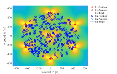
Figure 3: The layout of the UCN mMIMO system.

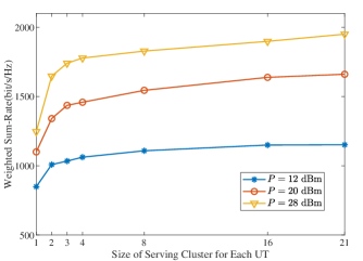
Figure 4: The relationship between the WSR performance and the size of the serving cluster.

First of all, we study the relationship between the WSR performance and the size of the serving cluster for each UT at different transmit powers in Fig. 4. As shown in Fig. 4, the WSR performance exhibits a decreasing rate of growth as the size of the serving cluster increases. This is because the BSs having the potential to provide greater service for each UT have been included in the serving cluster. The later the BS is selected into the serving cluster for each UT, the fewer contributions it will make to the WSR performance, and the more interference it could cause to its served group. At $P=28$ dBm, $P=20$ dBm and $P=12$ dBm, it is observed that in the UCN mMIMO system with $\mathrm{B}_{\mathrm{sc}}=21$, only 12%, 15% and 11% WSR performance gains can be achieved, respectively, at the cost of a sevenfold increase in computational complexities compared with the case with $\mathrm{B}_{\mathrm{sc}}=3$. Therefore, the UCN mMIMO system with $\mathrm{B}_{\mathrm{sc}}=3$ can achieve most of the WSR performance compared with the system with $\mathrm{B}_{\mathrm{sc}}=21$.

Then we investigate the WSR performances of the RCG method in comparison with the WMMSE and MRT methods at different transmit powers in Fig. 5. From Fig. 5, we see that the RCG method with $\mathrm{B}_{\mathrm{sc}}=1$ has the same performance as the popular WMMSE method with $\mathrm{B}_{\mathrm{sc}}=1$ [33]. While in the UCN mMIMO systems with $\mathrm{B}_{\mathrm{sc}}=3$ and $\mathrm{B}_{\mathrm{sc}}=21$, the RCG method all outperforms the WMMSE method [34] in the whole transmit power regime. It is worth noting that the RCG method has a much lower computational complexity than the WMMSE method per iteration for a given system, which shows the high efficiency of the RCG method. The MRT with $\mathrm{B}_{\mathrm{sc}}=3$ requires the least computational complexity but also exhibits the poorest performance. In addition, we observe that the RCG method with $\mathrm{B}_{\mathrm{sc}}=3$ performs much better than the case with $\mathrm{B}_{\mathrm{sc}}=1$ and has a 38% performance gain when $P=24$ dBm. Although the RCG method with $\mathrm{B}_{\mathrm{sc}}=21$ has the best performance, it suffers from the computational complexity that is seven times higher than that of the RCG method with $\mathrm{B}_{\mathrm{sc}}=3$. To show the high efficiency of the RCG method, we compare the complexities of the RCG method and the WMMSE method in the UCN system with $\mathrm{B}_{\mathrm{sc}}=3$ when the RCG method achieves the same performance as the converged WMMSE method. From Fig. 6, we observe that the RCG method needs to pay a much lower computational cost to achieve the same WSR performance as the WMMSE method that have converged. In addition, the RCG method avoids the inverses of large dimensional matrices and is more advantageous for the forthcoming 6G networks with more antennas equipped at the BS side.

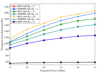
Figure 5: The WSR performance of the RCG method compared with the WMMSE method.

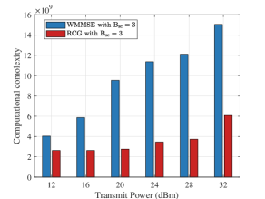
Figure 6: The complexities of the RCG method and the WMMSE method with $\mathrm{B}_{\mathrm{sc}}=3$ when they have the same performance.

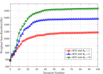
Figure 7: Convergence rate comparison between different configurations when $P=24$ dBm.

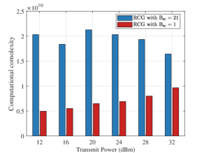
Figure 8: The complexities of the system with $\mathrm{B}_{\mathrm{sc}}=3$ and the system with $\mathrm{B}_{\mathrm{sc}}=21$ when they have the same performance.

We then study the convergence behavior of our proposed RCG method for precoder design of the UCN mMIMO. In Fig. 7, we plot the convergence trajectories of the RCG method when $P=24$ dBm with $\mathrm{B}_{\mathrm{sc}}$ taking different values. By observing Fig. 7, we can see that our method with $\mathrm{B}_{\mathrm{sc}}=3$ has achieved 85% WSR performance in the first 20 iterations and 93% performance in the first 30 iterations. The RCG method with $\mathrm{B}_{\mathrm{sc}}=3$ needs about $N=50$ iterations to converge, whose complexity is nearly the same as the RCG method with $\mathrm{B}_{\mathrm{sc}}=21$ when the number of iterations $N=7$. Although the two cases share nearly the same computational complexity, we can see from Fig. 7 that the system with $\mathrm{B}_{\mathrm{sc}}=3$ and $N=50$ has a large WSR performance gain compared with the system with $\mathrm{B}_{\mathrm{sc}}=21$ and $N=7$. Then, we compare the computational complexities of the RCG method when the system with $\mathrm{B}_{\mathrm{sc}}=21$ achieves the same performance as the converged system with $\mathrm{B}_{\mathrm{sc}}=3$ in Fig. 8. We see that the RCG method with $\mathrm{B}_{\mathrm{sc}}=3$ pays a lower computational cost to achieve the same performance as the case with $\mathrm{B}_{\mathrm{sc}}=21$.

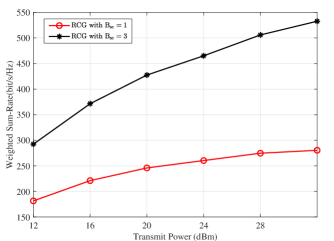
Figure 9: WSR performance of the cell-edge UTs.

To show the performance enhancement of the cell-edge UTs in the UCN mMIMO system, we compare the WSR performance of the cell-edge UTs in the system with $\mathrm{B}_{\mathrm{sc}}=1$ with the system with $\mathrm{B}_{\mathrm{sc}}=3$ in Fig. 9. The cell-edge UTs are defined as the UTs suffering higher interference from the adjacent cells according to [40]. From Fig. 9, we see that the system with $\mathrm{B}_{\mathrm{sc}}=3$ provides a much better WSR performance for cell-edge UTs than the system with $\mathrm{B}_{\mathrm{sc}}=1$ in the whole transmit power regime. Specifically, the cell-edge UTs have a 79% performance gain in the system with $\mathrm{B}_{\mathrm{sc}}=3$ compared with the system with $\mathrm{B}_{\mathrm{sc}}=1$ when $P=24$ dBm, showing the superiority of the UCN system with $\mathrm{B}_{\mathrm{sc}}=3$ in enhancing the WSR performance of the cell-edge UTs.

As a matter of fact, the UCN mMIMO system with $\mathrm{B}_{\mathrm{sc}}=1$ can be viewed as the cellular mMIMO system, and the UCN mMIMO system with $\mathrm{B}_{\mathrm{sc}}=21$ is equivalent to the conventional network mMIMO system. From the above simulation results, it can be inferred that $\mathrm{B}_{\mathrm{sc}}=3$ represents a favorable choice for the UCN mMIMO system to provide a good enough WSR performance with much reduced computational complexities. Compared with the cellular mMIMO system, the UCN mMIMO system with $\mathrm{B}_{\mathrm{sc}}=3$ can significantly enhance the WSR performance of the UTs in the system, especially for the cell-edge UTs. The computational complexity of the RCG method in the UCN mMIMO system with $\mathrm{B}_{\mathrm{sc}}=3$ is one-seventh of that in the conventional network system per outer iteration while exhibiting minimal performance degradation. Additionally, our proposed RCG method for precoder design obviates the need for inverting high-dimensional matrices, and exhibits a better WSR performance and a lower computational complexity compared with the WMMSE method. These results demonstrate the computational efficiency of the UCN mMIMO system with $\mathrm{B}_{\mathrm{sc}}=3$ and the numerical superiority of our proposed RCG method for precoder design.

VI Conclusion

In this paper, we have investigated the WSR-maximization precoder design for UCN mMIMO systems with matrix manifold optimization. In the UCN mMIMO system, the implementation cost of the system and the dimension of the precoder to be designed are much lower than those in the conventional network mMIMO system. By showing the precoders satisfying the power constraints of each BS are on a Riemannian submanifold, we transform the constrained WSR-maximization precoder design problem in Euclidean space to an unconstrained one on the Riemannian submanifold. By deriving all the Riemannian ingredients of the problem on the Riemannian submanifold, the RCG precoder design is proposed for solving the unconstrained problem. The proposed method does not involve the inverses of large dimensional matrices. In addition, the complexity analysis demonstrates the high efficiency of the proposed method. The numerical results not only confirm the superiority of the UCN mMIMO system, but also show significant performance gains and the high computational efficiency of the proposed RCG method for precoder design over the existing methods.

Appendix A Proof for Theorem 1

First, we show that $\mathcal{M}$ is an embedded submanifold of $\mathcal{N}$. Consider the differentiable function $F:\mathcal{N}\rightarrow\mathbb{R}^{B}:\mathbf{P}\mapsto F\left(\mathbf{P}\right)$, and (21) implies $\mathcal{M}=F^{-1}\left(\boldsymbol{0}_{B}\right)$, where $\boldsymbol{0}_{B}\in\mathbb{R}^{B}$. Based on the submersion theorem [30, Proposition 3.3.3], to show $\mathcal{M}$ is an embedded submanifold of $\mathcal{N}$, we need to prove $F$ as a submersion at each point of $\mathcal{M}$. In other words, we should verify that the rank of $F$ is equal to the dimension of $\mathbb{R}^{B}$, i.e., $B$, at every point of $\mathcal{M}$. Let $\mathbf{Z}=\mathbf{Z}_{1}\times\mathbf{Z}_{2}\times\cdots\times\mathbf{Z}_{U}$ be an arbitrary point on $\mathcal{N}$. Since the rank of $F$ at $\mathbf{P}\in\mathcal{N}$ is defined as the dimension of the range of $\mathrm{D}F\left(\mathbf{P}\right)$, we need to show that for all $\mathbf{w}\in\mathbb{R}^{B}$, there exists $\mathbf{Z}\in\mathcal{N}$ such that $\mathrm{D}F\left(\mathbf{P}\right)\left[\mathbf{Z}\right]=\mathbf{w}^{T}=\left(w_{1},w_{2},\cdots,w_{B}\right)$. Since the differential operation at $\mathbf{P}$ is equivalent to the component-wise differential at each of $\mathbf{P}_{1},\mathbf{P}_{2},\cdots,\mathbf{P}_{U}$, we have

$$\mathrm{D}F\left(\mathbf{P}\right)\left[\mathbf{Z}\right]= \Big{(}\sum_{k\in\mathcal{B}_{1}}2\Re\left\{\mathrm{tr}\left(\mathbf{P}_{1}^{H}\mathbf{W}_{1}^{H}\mathbf{Q}_{k}\mathbf{W}_{1}\mathbf{Z}_{1}\right)\right\},\cdots,$$ (63)

$$\sum_{k\in\mathcal{B}_{U}}2\Re\left\{\mathrm{tr}\left(\mathbf{P}_{U}^{H}\mathbf{W}_{U}^{H}\mathbf{Q}_{k}\mathbf{W}_{U}\mathbf{Z}_{U}\right)\right\}\Big{)}.$$

By choosing $\mathbf{Z}_{i}=\frac{1}{2}\frac{w_{k}}{P_{k}}\mathbf{P}_{i}$, we will have $\mathrm{D}F\left(\mathbf{P}\right)\left[\mathbf{Z}\right]=\mathbf{w}^{T}$. This shows that $F$ is full rank as well as a submersion on $\mathcal{M}$, and $\mathcal{M}$ is an embedded submanifold of $\mathcal{N}$.

In this case, $T_{\mathbf{P}}{\mathcal{M}}$ can be regarded as a subspace of $T_{\mathbf{P}}{\mathcal{N}}$, and the Riemannian metric $g_{\mathbf{P}}^{\mathcal{N}}\left(\cdot\right)$ on $\mathcal{N}$ naturally induces a Riemannian metric $g_{\mathbf{P}}^{\mathcal{M}}\left(\cdot\right)$ on $\mathcal{M}$ according to

$$g_{\mathbf{P}}^{\mathcal{M}}\left({\boldsymbol{\xi}}_{\mathbf{P}},{\boldsymbol{\zeta}}_{\mathbf{P}}\right)=g_{\mathbf{P}}^{\mathcal{N}}\left({\boldsymbol{\xi}}_{\mathbf{P}},{\boldsymbol{\zeta}}_{\mathbf{P}}\right),$$ (64)

where ${\boldsymbol{\xi}}_{\mathbf{P}}\in T_{\mathbf{P}}\mathcal{M}$ and ${\boldsymbol{\zeta}}_{\mathbf{P}}\in T_{\mathbf{P}}\mathcal{M}$ on the right hand side are viewed as elements in $T_{\mathbf{P}}\mathcal{N}$. With this metric, $\mathcal{M}$ is a Riemannian submanifold of $\mathcal{N}$.

Appendix B Proof for Lemma 1

With (29) and (28), we have

$${\boldsymbol{\Pi}}^{T_{\mathbf{P}}\mathcal{N}}_{T_{\mathbf{P}}\mathcal{M}}\left({\boldsymbol{\xi}}_{\mathbf{P}}\right)=\Big{(}{\boldsymbol{\xi}}_{\mathbf{P}_{1}}-\sum_{\ell\in\mathcal{B}_{1}}\mu_{\ell}\mathbf{W}_{1}^{H}\mathbf{Q}_{\ell}\mathbf{W}_{1}\mathbf{P}_{1},\cdots,$$ (65)

$${\boldsymbol{\xi}}_{\mathbf{P}_{U}}-\sum_{\ell\in\mathcal{B}_{U}}\mu_{\ell}\mathbf{W}_{U}^{H}\mathbf{Q}_{\ell}\mathbf{W}_{U}\mathbf{P}_{U}\Big{)}\in T_{\mathbf{P}}\mathcal{M},$$

which satisfies (27). So the equation

$$\sum_{i\in\mathcal{U}_{k}}\Re\Big{\{} \mathrm{tr}\Big{(}\big{(}{\boldsymbol{\xi}}_{\mathbf{P}_{i}}-\sum_{\ell\in\mathcal{B}_{i}}\mu_{\ell}\mathbf{W}_{i}^{H}\mathbf{Q}_{\ell}\mathbf{W}_{i}\mathbf{P}_{i}\big{)}^{H}$$ (66)

$$\times\mathbf{W}_{i}^{H}\mathbf{Q}_{k}\mathbf{W}_{i}\mathbf{P}_{i}\Big{)}\Big{\}}=0$$

holds for $k\in\mathcal{S}_{B}$. After some algebra, for $\ell\in\mathcal{S}_{B}$, we can get

$$\mu_{\ell}=\frac{1}{P_{\ell}}\sum_{i\in\mathcal{U}_{\ell}}\Re\left\{\mathrm{tr}\left(\mathbf{P}_{i}^{H}\mathbf{W}_{i}^{H}\mathbf{Q}_{\ell}\mathbf{W}_{i}{\boldsymbol{\xi}}_{\mathbf{P}_{i}}\right)\right\}.$$ (67)

Appendix C Proof for Theorem 2

Given that $\mathcal{N}$ is the product linear manifold composed of $\sum_{i\in\mathcal{S}_{U}}B_{i}$ complex vector spaces, $\mathrm{grad}_{\mathcal{N}}f\left(\mathbf{P}\right)$ only depends on $f\left(\mathbf{P}\right)$. For notational simplicity, we use $f\left(\mathbf{P}_{i}\right)$ to denote the objective function that only considers $\mathbf{P}_{i}$ as the optimization variable with $\mathbf{P}_{j},\forall j\neq i$, fixed. Similarly, let $f\left(\mathbf{P}_{i,k}\right)$ denote the objective function that only considers $\mathbf{P}_{i,k},k\in\mathcal{B}_{i},$ as the optimization variable with $\mathbf{P}_{j,\ell},\forall\left(j,\ell\right)\neq\left(i,k\right)$, fixed. $\mathrm{grad}_{\mathcal{N}}f\left(\mathbf{P}\right)$ is made up of $\mathrm{grad}_{\mathcal{N}_{i}}f\left(\mathbf{P}_{i}\right),\forall i\in\mathcal{S}_{U}$ as shown in (19) and $\mathrm{grad}_{\mathcal{N}_{i}}f\left(\mathbf{P}_{i}\right)$ is made up of $\mathrm{grad}_{\mathcal{N}_{i,k}}f\left(\mathbf{P}_{i,k}\right),\forall k\in\mathcal{B}_{i},$ as shown in (16). So we derive $\mathrm{grad}_{\mathcal{N}_{i,k}}f\left(\mathbf{P}_{i,k}\right)$ first. For any ${\boldsymbol{\xi}}_{\mathbf{P}_{i,k}}\in T_{\mathbf{P}_{i,k}}\mathcal{N}_{i,k}$, the directional derivative of $f\left(\mathbf{P}_{i,k}\right)$ along ${\boldsymbol{\xi}}_{\mathbf{P}_{i,k}}$ is

$$\mathrm{D}f\left(\mathbf{P}_{i,k}\right)\left[{\boldsymbol{\xi}}_{\mathbf{P}_{i,k}}\right]=$$ (68)

$$-w_{i}\mathrm{D}\mathcal{R}_{{i,k}}^{i}\left[{\boldsymbol{\xi}}_{\mathbf{P}_{i,k}}\right]-\sum_{j\neq i}^{U}w_{j}\mathrm{D}\mathcal{R}_{i,k}^{j}\left[{\boldsymbol{\xi}}_{\mathbf{P}_{i,k}}\right],i\in\mathcal{S}_{U},k\in\mathcal{S}_{B},$$

where $\mathcal{R}_{{i,k}}^{i}$ is the rate of UT $i$ that only considers $\mathbf{P}_{i,k}$ as the optimization variable and $\mathcal{R}_{i,k}^{{j}}$ is the rate of UT $j$ that only considers $\mathbf{P}_{i,k}$ as the optimization variable. $\mathcal{R}_{{i,k}}^{i}$ and $\mathcal{R}_{i,k}^{{j}}$ can be viewed as mappings from $\mathbb{C}^{M_{t}\times d_{i}}$ to $\mathbb{R}$, so $\mathrm{D}\mathcal{R}_{i,k}^{i}\left[{\boldsymbol{\xi}}_{\mathbf{P}_{i,k}}\right]$ and $\mathrm{D}\mathcal{R}_{i,k}^{j}\left[{\boldsymbol{\xi}}_{\mathbf{P}_{i,k}}\right]$ can be obtained from (26). We derive $\mathrm{D}\mathcal{R}_{i,k}^{i}\left[{\boldsymbol{\xi}}_{\mathbf{P}_{i,k}}\right]$ and $\mathrm{D}\mathcal{R}_{i,k}^{j}\left[{\boldsymbol{\xi}}_{\mathbf{P}_{i,k}}\right]$ separately as

$$\mathrm{D}\mathcal{R}_{i,k}^{i}\left[{\boldsymbol{\xi}}_{\mathbf{P}_{i,k}}\right]= \mathrm{tr}\bigg{(}\mathbf{C}_{i}\Big{(}{\boldsymbol{\xi}}_{\mathbf{P}_{i,k}}^{H}\mathbf{H}_{i,k}^{H}\mathbf{R}_{i}^{-1}\mathbf{H}_{i}\mathbf{W}_{i}\mathbf{P}_{i}+$$ (69)

$$\mathbf{P}_{i}^{H}\mathbf{W}_{i}^{H}\mathbf{H}_{i}^{H}\mathbf{R}_{i}^{-1}\mathbf{H}_{i,k}{\boldsymbol{\xi}}_{\mathbf{P}_{i,k}}\Big{)}\bigg{)}$$

$$= g_{\mathbf{P}_{i,k}}^{\mathcal{N}_{i,k}}\left(2\mathbf{H}_{i,k}^{H}\mathbf{R}_{i}^{-1}\mathbf{H}_{i}\mathbf{P}_{i}\mathbf{C}_{i},{\boldsymbol{\xi}}_{\mathbf{P}_{i,k}}\right),$$

$$\mathrm{D}\mathcal{R}_{i,k}^{j}\left[{\boldsymbol{\xi}}_{\mathbf{P}_{i,k}}\right] =-\mathrm{tr}\bigg{(}\mathbf{H}_{j,k}^{H}\mathbf{R}_{j}^{-1}\mathbf{H}_{j}\mathbf{W}_{j}\mathbf{P}_{j}\mathbf{C}_{j}\mathbf{P}_{j}^{H}\mathbf{W}_{j}^{H}\mathbf{H}_{j}^{H}$$ (70)

$$\times\mathbf{R}_{j}^{-1}\mathbf{H}_{j}\left({\boldsymbol{\xi}}_{\mathbf{P}_{i,k}}\mathbf{P}_{i}^{H}\mathbf{W}_{i}^{H}+\mathbf{W}_{i}\mathbf{P}_{i}{\boldsymbol{\xi}}_{\mathbf{P}_{i,k}}^{H}\right)\bigg{)}$$

$$= g_{\mathbf{P}_{i,k}}^{\mathcal{N}_{i,k}}\Big{(}-2\mathbf{H}_{j,k}^{H}\mathbf{R}_{j}^{-1}\mathbf{H}_{j}\mathbf{W}_{j}\mathbf{P}_{j}\mathbf{C}_{j}$$

$$\times\mathbf{P}_{j}^{H}\mathbf{W}_{j}^{H}\mathbf{H}_{j}^{H}\mathbf{R}_{j}^{-1}\mathbf{H}_{j}\mathbf{W}_{i}\mathbf{P}_{i},{\boldsymbol{\xi}}_{\mathbf{P}_{i,k}}\Big{)}.$$

Thus, we have

$$\mathrm{D}f\left(\mathbf{P}_{i,k}\right)\left[{\boldsymbol{\xi}}_{\mathbf{P}_{i,k}}\right]=g_{\mathbf{P}_{i,k}}^{\mathcal{N}_{i,k}}\big{(}{\boldsymbol{\xi}}_{\mathbf{P}_{i}},-2w_{i}\mathbf{H}_{i,k}^{H}\mathbf{R}_{i}^{-1}\mathbf{H}_{i}\mathbf{W}_{i}\mathbf{P}_{i}\mathbf{C}_{i}$$ (71)

$$+ 2\sum_{j\neq i}w_{j}\mathbf{H}_{j,k}^{H}\mathbf{R}_{j}^{-1}\mathbf{H}_{j}\mathbf{W}_{j}\mathbf{P}_{j}\mathbf{C}_{j}\mathbf{P}_{j}^{H}\mathbf{W}_{j}^{H}\mathbf{H}_{j}^{H}\mathbf{R}_{j}^{-1}\mathbf{H}_{j}\mathbf{W}_{i}\mathbf{P}_{i}\big{)}$$

and $\mathrm{grad}_{\mathcal{N}_{i,k}}f\left(\mathbf{P}_{i,k}\right)$ is

$$\mathrm{grad}_{\mathcal{N}_{i,k}}f\left(\mathbf{P}_{i,k}\right)=-2\big{(}w_{i}\mathbf{H}_{i,k}^{H}\mathbf{R}_{i}^{-1}\mathbf{H}_{i}\mathbf{W}_{i}\mathbf{P}_{i}\mathbf{C}_{i}$$ (72)

$$-\sum_{j\neq i}w_{j}\mathbf{H}_{j,k}^{H}\mathbf{R}_{j}^{-1}\mathbf{H}_{j}\mathbf{W}_{j}\mathbf{P}_{j}\mathbf{C}_{j}\mathbf{P}_{j}^{H}\mathbf{W}_{j}^{H}\mathbf{H}_{j}^{H}\mathbf{R}_{j}^{-1}\mathbf{H}_{j}\mathbf{W}_{i}\mathbf{P}_{i}\big{)}.$$

With (16), (19) and (72), $\mathrm{grad}_{\mathcal{N}}f\left(\mathbf{P}\right)$ can be easily obtained. With [30, Theorem 3.6.1] and Lemma 1, the Riemannian gradient of $f\left(\mathbf{P}\right)$ in $T_{\mathbf{P}}\mathcal{M}$ is

$$\mathrm{grad}_{\mathcal{M}} f\left(\mathbf{P}\right)={\boldsymbol{\Pi}}_{T_{\mathbf{P}}\mathcal{M}}^{T_{\mathbf{P}}\mathcal{N}}\left(\mathrm{grad}_{\mathcal{N}}f\left(\mathbf{P}\right)\right)$$ (73)

$$=\Big{(} \mathrm{grad}_{\mathcal{N}_{1}}f\left(\mathbf{P}_{1}\right)-\sum_{k\in\mathcal{B}_{1}}\lambda_{k}\mathbf{W}_{1}^{H}\mathbf{Q}_{k}\mathbf{W}_{1}\mathbf{P}_{1},\cdots,$$

$$\mathrm{grad}_{\mathcal{N}_{U}}f\left(\mathbf{P}_{U}\right)-\sum_{k\in\mathcal{B}_{U}}\lambda_{k}\mathbf{W}_{U}^{H}\mathbf{Q}_{k}\mathbf{W}_{U}\mathbf{P}_{U}\Big{)},$$

where

$$\lambda_{k}=\frac{1}{P_{k}}\sum_{i\in\mathcal{U}_{k}}\Re\left\{\mathrm{tr}\left(\mathbf{P}_{i}^{H}\mathbf{W}_{i}^{H}\mathbf{Q}_{k}\mathbf{W}_{i}\mathrm{grad}_{\mathcal{N}_{i}}f\left(\mathbf{P}_{i}\right)\right)\right\}.$$ (74)

Appendix D Proof for Theorem 4

From [30, Section 8.1.3], the vector transport for a Riemannian submanifold of a Euclidean space can be defined by the orthogonal projection, based on which the vector transport is the orthogonal projection from $T_{\mathbf{P}}\mathcal{M}$ to $T_{\mathbf{P}^{\mathrm{new}}}\mathcal{M}$. We have obtained the orthogonal projection from $T_{\mathbf{P}}\mathcal{N}$ to $T_{\mathbf{P}}\mathcal{M}$ in Lemma 1 based on that $T_{\mathbf{P}}\mathcal{N}$ can be decomposed into two orthogonal spaces. Given that $T_{\mathbf{P}}\mathcal{M}$ is a subspace of $T_{\mathbf{P}}\mathcal{N}=\mathbb{C}^{B_{1}M_{t}\times d_{1}}\times\cdots\times\mathbb{C}^{B_{U}M_{t}\times d_{U}}=T_{\mathbf{P}^{\mathrm{new}}}\mathcal{N}$, $T_{\mathbf{P}}\mathcal{M}$ can also be decomposed as

$$T_{\mathbf{P}}\mathcal{M}=T_{\mathbf{P}^{\mathrm{new}}}^{\mathrm{sub}}\mathcal{M}\oplus N_{\mathbf{P}^{\mathrm{new}}}^{\mathrm{sub}}\mathcal{M},$$ (75)

where $T_{\mathbf{P}^{\mathrm{new}}}^{\mathrm{sub}}\mathcal{M}$ and $N_{\mathbf{P}^{\mathrm{new}}}^{\mathrm{sub}}\mathcal{M}$ are the subspaces of the tangent space and the normal space of $\mathcal{M}$ at $\mathbf{P}^{\mathrm{new}}$, respectively. From (28), we have

$$N_{\mathbf{P}^{\mathrm{new}}}^{\mathrm{sub}}\mathcal{M}= \Big{\{}\Big{(}\sum_{\ell\in\mathcal{B}_{1}}\mu_{\ell}\mathbf{W}_{1}^{H}\mathbf{Q}_{\ell}\mathbf{W}_{1}\mathbf{P}_{1}^{\mathrm{new}},\cdots,$$ (76)

$$\sum_{\ell\in\mathcal{B}_{U}}\mu_{\ell}\mathbf{W}_{U}^{H}\mathbf{Q}_{\ell}\mathbf{W}_{U}\mathbf{P}_{U}^{\mathrm{new}}\Big{)}\mid\rho_{\ell}\in\mathbb{R},\mathbf{P}\in\mathcal{M}\Big{\}}.$$

From (75) and (76), the vector transport can be defined as

$$\mathcal{T}_{\boldsymbol{\eta}_{\mathbf{P}}}^{\mathcal{M}}\left({\boldsymbol{\xi}}_{\mathbf{P}}\right)= {\boldsymbol{\Pi}}^{T_{\mathbf{P}}\mathcal{M}}_{T_{\mathbf{P}^{\mathrm{new}}}\mathcal{M}}\left({\boldsymbol{\xi}}_{\mathbf{P}}\right)={\boldsymbol{\Pi}}^{T_{\mathbf{P}}\mathcal{M}}_{T_{\mathbf{P}^{\mathrm{new}}}^{\mathrm{sub}}\mathcal{M}}\left({\boldsymbol{\xi}}_{\mathbf{P}}\right)$$ (77)

$$= \Big{(}{\boldsymbol{\xi}}_{\mathbf{P}_{1}}-\sum_{\ell\in\mathcal{S}_{B}}\rho_{\ell}\mathbf{W}_{1}^{H}\mathbf{Q}_{\ell}\mathbf{W}_{1}\mathbf{P}^{\mathrm{new}}_{1},\cdots,$$

$${\boldsymbol{\xi}}_{\mathbf{P}_{U}}-\sum_{\ell\in\mathcal{S}_{B}}\rho_{\ell}\mathbf{W}_{U}^{H}\mathbf{Q}_{\ell}\mathbf{W}_{U}\mathbf{P}^{\mathrm{new}}_{U}\Big{)}.$$

As $T_{\mathbf{P}^{\mathrm{new}}}^{\mathrm{sub}}\mathcal{M}\subseteq T_{\mathbf{P}^{\mathrm{new}}}\mathcal{M}$, $\left({\boldsymbol{\xi}}_{\mathbf{P}}-\sum_{\ell\in\mathcal{S}_{B}}\rho_{\ell}\mathbf{Q}_{\ell}\mathbf{P}^{\mathrm{new}}\right)$ should satisfy

$$\sum_{i\in\mathcal{U}_{k}}\Re \Big{\{}\mathrm{tr}\Big{(}\left(\mathbf{P}_{i}^{\mathrm{new}}\right)^{H}\mathbf{W}_{i}^{H}\mathbf{Q}_{k}\mathbf{W}_{i}$$ (78)

$$\times\big{(}{\boldsymbol{\xi}}_{\mathbf{P}_{i}}-\sum_{\ell\in\mathcal{S}_{B}}\rho_{\ell}\mathbf{W}_{i}^{H}\mathbf{Q}_{\ell}\mathbf{W}_{i}\mathbf{P}_{i}^{\mathrm{new}}\big{)}\Big{)}\Big{\}}=0$$

After some algebra, we can get

$$\rho_{\ell}=\frac{1}{P_{\ell}}\sum_{i\in\mathcal{U}_{\ell}}\Re\left\{\mathrm{tr}\left(\left(\mathbf{P}^{\mathrm{new}}_{i}\right)^{H}\mathbf{W}_{i}^{H}\mathbf{Q}_{\ell}\mathbf{W}_{i}{\boldsymbol{\xi}}_{\mathbf{P}_{i}}\right)\right\},\ell\in\mathcal{S}_{B}.$$ (79)

References

• [1] C.-X. Wang, X. You, X.-Q. Gao, X. Zhu, Z. Li, C. Zhang, H. Wang, Y. Huang, Y. Chen, H. Haas et al., “On the road to 6G: Visions, requirements, key technologies and testbeds,” IEEE Commun. Surv. Tutor., 2023.
• [2] R. M. Dreifuerst and R. W. Heath, “Massive MIMO in 5G: How beamforming, codebooks, and feedback enable larger arrays,” IEEE Commun. Mag., vol. 61, no. 12, pp. 18–23, 2023.
• [3] H. Jin, K. Liu, M. Zhang, L. Zhang, G. Lee, E. N. Farag, D. Zhu, E. Onggosanusi, M. Shafi, and H. Tataria, “Massive MIMO evolution towards 3GPP release 18,” IEEE J. Sel. Areas Commun., 2023.
• [4] A.-A. Lu, Y. Chen, and X. Gao, “2D beam domain statistical CSI estimation for massive MIMO uplink,” IEEE Trans. Wireless Commun., vol. 23, no. 1, pp. 749–761, Jan. 2024.
• [5] L. You, J. Xu, G. C. Alexandropoulos, J. Wang, W. Wang, and X. Gao, “Energy efficiency maximization of massive MIMO communications with dynamic metasurface antennas,” IEEE Trans. Wireless Commun., vol. 22, no. 1, pp. 393–407, Jan. 2023.
• [6] L. You, K.-X. Li, J. Wang, X.-Q. Gao, X.-G. Xia, and B. Ottersten, “Massive MIMO transmission for LEO satellite communications,” IEEE J. Sel. Areas Commun., vol. 38, no. 8, pp. 1851–1865, Jun. 2020.
• [7] M. Rahman and H. Yanikomeroglu, “Enhancing cell-edge performance: a downlink dynamic interference avoidance scheme with inter-cell coordination,” IEEE Trans. Wireless Commun., vol. 9, no. 4, pp. 1414–1425, Apr. 2010.
• [8] L. You, X. Chen, X. Song, F. Jiang, W. Wang, X.-Q. Gao, and G. Fettweis, “Network massive mimo transmission over millimeter-wave and terahertz bands: Mobility enhancement and blockage mitigation,” IEEE J. Sel. Areas Commun., vol. 38, no. 12, pp. 2946–2960, Dec. 2020.
• [9] S. Venkatesan, A. Lozano, and R. Valenzuela, “Network MIMO: Overcoming intercell interference in indoor wireless systems,” in 2007 Conference Record of the Forty-First Asilomar Conference on Signals, Systems and Computers, 2007, pp. 83–87.
• [10] C. Lee, C.-B. Chae, T. Kim, S. Choi, and J. Lee, “Network massive MIMO for cell-boundary users: From a precoding normalization perspective,” in 2012 IEEE Globecom Workshops, 2012, pp. 233–237.
• [11] J. Zhang, S. Chen, Y. Lin, J. Zheng, B. Ai, and L. Hanzo, “Cell-free massive MIMO: A new next-generation paradigm,” IEEE Access, vol. 7, pp. 99 878–99 888, 2019.
• [12] S. Elhoushy, M. Ibrahim, and W. Hamouda, “Cell-free massive mimo: A survey,” IEEE Commun. Surv. Tutor., vol. 24, no. 1, pp. 492–523, 2022.
• [13] H. I. Obakhena, A. L. Imoize, F. I. Anyasi, and K. Kavitha, “Application of cell-free massive MIMO in 5G and beyond 5G wireless networks: A survey,” Journal of Engineering and Applied Science, vol. 68, no. 1, pp. 1–41, 2021.
• [14] I. Kanno, K. Yamazaki, Y. Kishi, and S. Konishi, “A survey on research activities for deploying cell free massive MIMO towards beyond 5G,” IEICE Trans. Commun., vol. 105, no. 10, pp. 1107–1116, 2022.
• [15] S. Chen, L. Chen, B. Hu, S. Sun, Y. Wang, H. Wang, and W. Gao, “User-centric access network (UCAN) for 6G: Motivation, concept, challenges and key technologies,” IEEE Network, 2023.
• [16] L. Qin, H. Lu, and F. Wu, “When the user-centric network meets mobile edge computing: Challenges and optimization,” IEEE Communications Magazine, vol. 61, no. 1, pp. 114–120, 2022.
• [17] H. A. Ammar, R. Adve, S. Shahbazpanahi, G. Boudreau, and K. V. Srinivas, “User-centric cell-free massive MIMO networks: A survey of opportunities, challenges and solutions,” IEEE Commun. Surv. Tutor., vol. 24, no. 1, pp. 611–652, Firstquarter 2022.
• [18] X. Lai, J. Xia, L. Fan, T. Q. Duong, and A. Nallanathan, “Outdated access point selection for mobile edge computing with cochannel interference,” IEEE Trans. Veh. Technol., vol. 71, no. 7, pp. 7445–7455, Jul. 2022.
• [19] M. A. Albreem, A. H. Al Habbash, A. M. Abu-Hudrouss, and S. S. Ikki, “Overview of precoding techniques for massive MIMO,” IEEE Access, vol. 9, pp. 60 764–60 801, 2021.
• [20] J. Shi, A.-A. Lu, W. Zhong, X. Gao, and G. Y. Li, “Robust WMMSE precoder with deep learning design for massive MIMO,” IEEE Trans. Commun., vol. 71, no. 7, pp. 3963–3976, Jul. 2023.
• [21] X. Yu, X. Gao, A.-A. Lu, J. Zhang, H. Wu, and G. Y. Li, “Robust precoding for HF skywave massive MIMO,” IEEE Trans. Wireless Commun., vol. 22, no. 10, pp. 6691–6705, Oct. 2023.
• [22] Q. Shi, M. Razaviyayn, Z.-Q. Luo, and C. He, “An iteratively weighted MMSE approach to distributed sum-utility maximization for a MIMO interfering broadcast channel,” IEEE Trans. Signal Process., vol. 59, no. 9, pp. 4331–4340, Sep. 2011.
• [23] C. Ding, J.-B. Wang, H. Zhang, M. Lin, and G. Y. Li, “Joint MIMO precoding and computation resource allocation for dual-function radar and communication systems with mobile edge computing,” IEEE J. Sel. Areas Commun., vol. 40, no. 7, pp. 2085–2102, Jul. 2022.
• [24] Y. Yuan, R. He, B. Ai, Z. Ma, Y. Miao, Y. Niu, J. Zhang, R. Chen, and Z. Zhong, “A 3D geometry-based THz channel model for 6G ultra massive MIMO systems,” IEEE Transactions on Vehicular Technology, vol. 71, no. 3, pp. 2251–2266, Mar. 2022.
• [25] E. Shtaiwi, H. Zhang, A. Abdelhadi, A. Lee Swindlehurst, Z. Han, and H. Vincent Poor, “Sum-rate maximization for RIS-assisted integrated sensing and communication systems with manifold optimization,” IEEE Trans. Commun., pp. 1–1, 2023.
• [26] C.-p. Lee, “Accelerating inexact successive quadratic approximation for regularized optimization through manifold identification,” Math. Program., pp. 1–35, 2023.
• [27] T. Osa, “Motion planning by learning the solution manifold in trajectory optimization,” Int. J. Rob. Res., vol. 41, no. 3, pp. 281–311, 2022.
• [28] Q. Le, Q. Shi, Q. Liu, X. Yao, X. Ju, and C. Xu, “Numerical investigation on manifold immersion cooling scheme for lithium ion battery thermal management application,” Int. J. Heat Mass Trans., vol. 190, p. 122750, 2022.
• [29] J. Choi, Y. Cho, and B. L. Evans, “Quantized massive MIMO systems with multicell coordinated beamforming and power control,” IEEE Trans. Commun., vol. 69, no. 2, pp. 946–961, Feb. 2021.
• [30] P.-A. Absil, R. Mahony, and R. Sepulchre, Optimization Algorithms on Matrix Manifolds.   Princeton University Press, 2009.
• [31] J. Nocedal and S. J. Wright, Numerical Optimization.   Springer, 1999.
• [32] H. Sato, “Riemannian conjugate gradient methods: General framework and specific algorithms with convergence analyses,” SIAM J. Optim., vol. 32, no. 4, pp. 2690–2717, 2022.
• [33] Q. Shi, M. Razaviyayn, Z.-Q. Luo, and C. He, “An iteratively weighted MMSE approach to distributed sum-utility maximization for a MIMO interfering broadcast channel,” IEEE Trans. Signal Process., vol. 59, no. 9, pp. 4331–4340, Sep. 2011.
• [34] Z. Wu and Z. Fei, “Precoder design in downlink CoMP-JT MIMO network via WMMSE and asynchronous ADMM,” Science China Information Sciences, vol. 61, pp. 1–13, 2018.
• [35] S. Jaeckel, L. Raschkowski, K. Borner, and L. Thiele, “Quadriga: A 3-D multi-cell channel model with time evolution for enabling virtual field trials,” IEEE Trans. Antennas Propag., vol. 62, no. 6, pp. 3242–3256, Jun. 2014.
• [36] 3GPP, “NR and NG-RAN overall description,” 3rd Generation Partnership Project (3GPP), Technical Specification (TS) 38.300, 10 2023, version 17.6.0.
• [37] 3GPP, “Base Station (BS) radio transmission and reception,” 3rd Generation Partnership Project (3GPP), Technical Specification (TS) 38.104, 07 2023, version 17.10.0.
• [38] 3GPP, “Study on channel model for frequencies from 0.5 to 100 GHz,” 3rd Generation Partnership Project (3GPP), Technical Report (TR) 38.901, 04 2022, version 17.0.0.
• [39] N. Fatema, G. Hua, Y. Xiang, D. Peng, and I. Natgunanathan, “Massive MIMO linear precoding: A survey,” IEEE Systems Journal, vol. 12, no. 4, pp. 3920–3931, 2018.
• [40] H. R. Chayon, K. B. Dimyati, H. Ramiah, and A. W. Reza, “Enhanced quality of service of cell-edge user by extending modified largest weighted delay first algorithm in LTE networks,” Symmetry, vol. 9, no. 6, p. 81, 2017.