Schrödinger’s bridges with stopping: Steering of stochastic flows towards spatio-temporal marginals

Abstract

In a gedanken experiment, in 1931/32, Erwin Schrödinger sought to understand how unlikely events can be reconciled with prior laws dictated by the underlying physics. In the process, he posed and solved a celebrated problem that is now named after him – the Schrödinger’s bridge problem (SBP). In this, one seeks to find the “most likely” path that stochastic particles took while transitioning between states probabilistically incompatible with the prior. Schrödinger’s problem proved to have yet another interpretation, that of the stochastic control problem to steer diffusive particles by a suitable control action so as to match specified marginals – a soft probabilistic constraint. Interestingly, the SBP is convex and can be solved by an efficient iterative algorithm known as the Fortet-Sinkhorn algorithm. The dual interpretation of the SBP, as an estimation and a control problem, as well as its computational tractability, are at the heart of an ever-expanding range of applications in controls. The purpose of the present work is to expand substantially the type of control and estimation problems that can be addressed following Schrödinger’s dictum, by incorporating stopping (freezing) of a given stochastic flow. Specifically, in the context of estimation, we seek the most likely evolution realizing prescribed spatio-temporal marginals of stopped particles. In the context of control, we seek the control action directing the stochastic flow toward spatio-temporal probabilistic constraints. To this end, we derive a new Schrödinger system of coupled, in space and time, partial differential equations to construct the solution of the proposed problem. Further, we show that a Fortet-Sinkhorn type of algorithm is, once again, available to attain the associated bridge. A key feature of the framework is that the obtained bridge retains the Markovian structure in the prior process, and thereby, the corresponding control action takes the form of state feedback.

Stochastic optimal control, Schrödinger bridges, Large deviations theory, Stopped processes.

1 Introduction

In two influential treatises [1, 2], E. Schrödinger detailed his thoughts on the time symmetry of the laws of nature (“Über die Umkehrung der Naturgesetze”). Schrödinger’s ultimate goal was to understand his namesake equation and the weirdness of the quantum world in classical terms. In the referred work, he began with a gedanken experiment to understand how measured atypical events can be reconciled with a prior law. Amid his perusal, Schrödinger single-handedly posed and solved the currently known as the Schrödinger’s bridge problem (SBP). The problem aims to determine the most likely trajectories of particles, as these transition between states, that are inconsistent with an underlying prior law. More formally, one seeks a posterior distribution on paths that interpolates, i.e. “bridges”, end-point marginals obtained empirically.

In the same work, Schrödinger quantified the likelihood of rare events with the relative entropy between the empirical distribution and the prior, thereby anticipating the development of the theory of large deviations [3]. Furthermore, he discovered a number of now-familiar control concepts, including a system of a Fokker-Planck equation and its adjoint, coupled at the boundaries, that is nowadays referred to as a Schrödinger system. The optimal solution to the SBP, Schrödinger concluded, can be obtained by alternatingly solving the two partial differential equations till convergence. This approach was rigorously proven a few years later by R. Fortet [4], and the iterative procedure is now known as the Fortet-Sinkhorn algorithm [5].

In hindsight, it seems astonishing that the control theoretic nature of Schrödinger’s problem was not recognized until sixty years later, when, in a masterful work [6], P. Dai Pra utilized Flemming’s logarithmic transformation to link the SBP with the minimal-energy stochastic-control problem of steering a stochastic system between two endpoint marginals. Fast forward another twenty years with the thesis of Y. Chen [7] and several related works [8, 9, 10, 11, 12, 13], and the SBP began taking up its rightful place within the stochastic control literature. Indeed, the relation between Schrödinger’s problem and the rapidly developing theory of Monge-Kantorovich optimal mass transport must not be overlooked. We refer to [14, 5, 15, 16, 17] for an overview of current developments. Due to the aforementioned dual interpretation and computational tractability, the SBP offers a wide range of applications in control and several neighboring fields e.g. estimation [18], physics [19], and machine learning [20, 21].

The present work aims to shed light on a new type of control and estimation problems that can be addressed following Schrödinger’s rationale. The problem at hand considers stochastic particles that diffuse while some particles can stop, or equivalently freeze in place. Within this setting, the concerned marginals are the particles’ initial distribution in space and the spatio-temporal marginal of the stopped particles over a bounded time horizon. Essentially, the stopped diffusion of particles can model a stochastic system completing a task. Then, our control problem seeks to determine the optimal control action, in the sense of Schrödinger, of the stochastic system and the required stopping rate to satisfy both the initial and spatio-temporal marginal constraints. The dual estimation problem likewise seeks the most likely evolution to bridge the same initial and spatio-temporal marginals.

The joint densities of location and time of stopping, e.g. location and time of sediment deposition (effectively mass loss as will be discussed later) for a diffusive flow of particles, are data that our framework aims to incorporate. Our goal is to infer the probabilistic model explaining the data and, on the flip side, determine the required added drift (feedback controller) and stopping rate to fulfill given spatio-temporal marginal requirements. In this work, we detail a new Schrödinger system of coupled partial differential equations allowing for constructing solutions to such problems. Moreover, we present an apprehensible Fortet-Sinkhorn type of algorithm to numerically attain solutions.

The paper is structured as follows: In Section 2, we lay out the newly proposed problem and its mathematical formulation as a large deviations problem given a Markov prior law. In Section 3, we present the rationale for establishing the solution to the large deviations problem by deriving a new suitable Schrödinger system. Section 4 discusses the numerical computation of the solution, via a special Fortet-Sinkhorn iteration that reflects the space-time structure of the problem. Before concluding, a numerical example is provided in Section 5.

2 Problem Description and Formalism

The starting point of our problem formulation can be traced to [22] and [18]. The first paper introduces a variation of Schrödinger’s problem where losses along trajectories of diffusive particles result in unbalanced masses of the two endpoint marginals. The second paper develops a model for random losses on a Markov chain, in discrete time and space, where marginals are available on stopping times at specific sites (states). The present work builds on this idea – to develop a model for controlled stochastic dynamics that may terminate over a bounded time horizon with the aim to regulate the stopping spatio-temporal profile. In that sense, the probability law weighs in on trajectories of possibly different lengths.

For notational and analysis purposes, it is convenient to extend trajectories beyond stopping by freezing the value of the state. This can be done in a way trajectories experience a discontinuity in dynamics. In turn, it is mathematized by having a first segment evolving in a primary state space and when stopped, the particles settle in a shadow state-space where dynamics have vanishing drift and stochastic excitation. Bear in mind that the primary and shadow spaces can coexist in the same physical space. However, such an abstraction helps to model the dynamics of the particles that never stop, i.e. exclusively exist in the primary space over the time window, as a diffusion with a killing rate. We refer to [23] for an interesting exposition about killed processes.

To this end, we define a “fused” state space that comprises a primary Euclidean state-space ${\mathcal{X}}_{\rm p}=\mathbb{R}^{n}$ and a “shadow” replica ${\mathcal{X}}_{\rm s}=\mathbb{R}^{n}$ where stopped particles reside. That is, the stochastic process is meant to evolve in the augmented space

$${\mathcal{X}}:={\mathcal{X}}_{\rm p}\cup{\mathcal{X}}_{\rm s},$$

see Figure 1 for a pictorial representation. Throughout, we consider time in the bounded window $[0,1]$ to evaluate probabilities of the continuation in ${\mathcal{X}}_{\rm p}$ (survival) or migration to ${\mathcal{X}}_{\rm s}$ (termination). Trajectories in the fused space can be metrized by the Skorohod metric [24, 25], where curves are compared by how much they need to be perturbed in both the domain (i.e., the time axis) and range, to match.

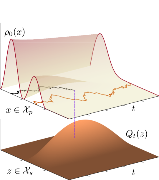
Figure 1: Illustration of diffusion with losses: The top sub-figure shows the primary space ${\mathcal{X}}_{p}$ that supports the diffusive trajectories of particles along with a drawing of the initial marginal distribution $\rho_{0}$ and also of the final marginal. The bottom sub-figure shows the spatio-temporal marginal $Q_{t}$ of stopped particles as they accumulate in the shadow space ${\mathcal{X}}_{s}$.

The space of concerned sample paths will be denoted by $\Omega$, namely $\Omega:=\mathbf{D}([0,1],{\mathcal{X}})$ where $\mathbf{D}$ is the Skorokhod space over ${\mathcal{X}}$. The prior law on $\Omega$ is denoted by ${\mathbf{R}}$ and corresponds to a Markov stochastic process ${\mathbf{X}}_{t}$ taking values in ${\mathcal{X}}$. The first component of ${\mathbf{X}}_{t}$ (i.e. the process restricted to ${\mathcal{X}}_{\rm p}$) evolves according to

$$dX_{t}=b(t,X_{t})dt+\sigma(t,X_{t})dW_{t},$$ (1)

while the second component takes values in ${\mathcal{X}}_{\rm s}$ and corresponds to the trivial dynamics $dZ_{t}=0$. Under the prior dynamics, the transition between components (here, from the first to the second) takes place due to some killing rate $V>0$, which can be a function of both time and space. Accordingly, from (1), if ${\mathbf{R}}_{t}$ denotes the one-time marginal of ${\mathbf{R}}$ and the restriction of ${\mathbf{R}}_{t}$ to the first component is denoted as $R_{t}$, then $R_{t}$ satisfies

$$\partial_{t}R_{t}=-\nabla\cdot(bR_{t})+\frac{1}{2}\sum_{i,j=1}^{n}\frac{\partial^{2}(a_{i,j}R_{t})}{\partial x_{i}\partial x_{j}}-VR_{t},$$ (2)

where $a:=\sigma\sigma^{\prime}$ is a positive definite matrix. Equation (2) is the Fokker-Planck equation with a killing rate $V$. Equivalently,

$$R_{t}(\cdot)=\int r(0,x,t,\cdot)R_{0}(x)dx,$$ (3)

where $r(0,x,t,y)$ denotes the Markov transition kernel from $x\in{\mathcal{X}}_{\rm p}$ at time equals $0$ to $y\in{\mathcal{X}}_{\rm p}$ at time $t$.

Thus, in this letter, we consider the control problem to specify the optimal update for both the drift and the killing rate of ${\mathbf{X}}_{t}$, so as to ensure suitable deposition-related marginal at different times. In turn, the data for our problem is the spatio-temporal marginal associated with particles that migrated to the shadow space, denoted by $Q_{t}(z)$ for $z\in{\mathcal{X}}_{\rm s},t\in[0,1]$, together with the initial probability density at ${\mathbf{X}}_{0}$. Assuming the prior is inconsistent with the data, from the estimation perspective, we seek to update the prior law ${\mathbf{R}}$ with an optimal posterior that reconciles with the data. Any candidate (i.e. consistent) posterior law is denoted as ${\mathbf{P}}$ and has a one-time marginal denoted by ${\mathbf{P}}_{t}$. The restriction of ${\mathbf{P}}_{t}$ to the first component of ${\mathcal{X}}={\mathcal{X}}_{\rm p}\cup{\mathcal{X}}_{\rm s}$ is denoted by $P_{t}$. The optimal posterior ${\mathbf{P}}^{\star}$, in the sense of Schrödinger, is the one closest to ${\mathbf{R}}$ apropos to a relative entropy functional and matches the data. For that, we propose the following problem.

Problem 1

(Spatio-Temporal Stopping Data) Given a prior Markov law ${\mathbf{R}}$ with one-time marginals restricted to the first component evolve according to (2), a probability density $\rho_{0}$ with support in ${\mathcal{X}}_{\rm p}$ and a spatio-temporal marginal $Q_{t}$ with support in ${\mathcal{X}}_{\rm s}\times[0,1]$, determine

$${\mathbf{P}}^{\star}:=\arg\min_{{\mathbf{R}}\gg{\mathbf{P}}} \mathbb{D}({\mathbf{P}}\parallel{\mathbf{R}})=\int_{\Omega}d{\mathbf{P}}\log\frac{d{\mathbf{P}}}{d{\mathbf{R}}},$$ (4a)

$$\mbox{ subject to }{\mathbf{P}}_{0}(x) =\rho_{0}(x),\ \text{for }x\in{\mathcal{X}}_{\rm p},$$ (4b)

$$\mbox{and }{\mathbf{P}}_{t}(x) =Q_{t}(x),\ \text{for }x\in{\mathcal{X}}_{\rm s}.$$ (4c)

The objective functional in (4a) is the relative entropy between ${\mathbf{P}}$ and ${\mathbf{R}}$. It is strictly convex and bounded when ${\mathbf{P}}$ is absolutely continuous with respect to ${\mathbf{R}}$, a relation denoted by ${\mathbf{R}}\gg{\mathbf{P}}$ [26]. The specification in (4b) amounts to the simplifying assumption that no particles are stopped initially since $\int_{{\mathcal{X}}_{{\rm p}}}\rho_{0}(x)dx=1$; thus, for consistency, we take $Q_{t=0}(\cdot)=0$. Due to our formalism, (4c) can be rewritten as

$$\alpha(t,x)V(t,x)P_{t}(x)=Q_{t}(x),$$ (4c’)

where $\alpha(t,x)V(t,x)$ is the killing rate corresponding to ${\mathbf{P}}^{\star}$ and $\alpha$ is the optimal update over the prior killing rate $V$.

A pictorial for the law that is being sought in Problem 1 is drawn in Figure 1. In this, the process ${\mathbf{X}}_{t}$ represents stochastic particles that drift along with the chance of being deposited at some location, say $z$ at time $t$. Then, when ${\mathbf{X}}_{t}$ takes values in ${\mathcal{X}}_{\rm s}$, it is seen as sediment that has been deposited (stopped). When ${\mathbf{X}}_{t}$ remains in ${\mathcal{X}}_{\rm p}$ for the duration, the corresponding particles remain in transit throughout. A control theoretic significance for Problem 1 stems from applications involving agents that obey stochastic dynamics until they complete a task, at which point they stop; the added drift represents control/steering whereas the killing rate represents the likelihood of completing the required task at location $z$ and time $t$. Thus, Problem 1 amounts to both, the control problem to update control action and rate of completion so as to match specifications, as well as the modeling problem to update values for drift and losses that match a given $Q_{t}(\cdot)$.

3 Establishing the Solution

In this section, we derive the Schrödinger system corresponding to Problem 1. We start by looking into the objective functional (4a) that decomposes as

$$\mathbb{D}({\mathbf{P}}\parallel{\mathbf{R}})=\int_{\Omega_{\rm p}}d{\mathbf{P}}\log\frac{d{\mathbf{P}}}{d{\mathbf{R}}}+\int_{\Omega_{\rm s}}d{\mathbf{P}}\log\frac{d{\mathbf{P}}}{d{\mathbf{R}}},$$

where the symbol $\Omega_{\rm p}$ denotes the space of sample paths of surviving particles over the time horizon $[0,1]$, and the set $\Omega_{\rm s}:=\Omega\setminus\Omega_{\rm p}$ is its complement. It is useful to note that $\Omega_{s}$ is a union of disjoint sets with each being a subset of sample paths of particles that stopped at some location $z$ at instant $t$.

We now define

$${\mathbf{P}}_{0,x}^{1,y}(\cdot) :={\mathbf{P}}(.|{\mathbf{X}}_{0}=x,{\mathbf{X}}_{1}=y),$$

$${\mathbf{P}}_{0,x}^{t,z}(\cdot) :={\mathbf{P}}(.|{\mathbf{X}}_{0}=x,{\mathbf{X}}_{t}=z),$$

for any $x\in{\mathcal{X}}_{\rm p},y\in{\mathcal{X}}_{\rm p},z\in{\mathcal{X}}_{\rm s},t\in[0,1]$. The conditioning ${\mathbf{P}}_{0,x}^{1,y}$/${\mathbf{P}}_{0,x}^{t,z}$ describes the disintegration of ${\mathbf{P}}$ with respect to the initial and final/freezing positions in the primary/shadow space. Moreover, we let their respective disintegrated counterparts of ${\mathbf{R}}$ be ${\mathbf{R}}_{0,x}^{1,y}$ and ${\mathbf{R}}_{0,x}^{t,z}$. Then, using the disintegration theorem [27] and the chain rule of conditional probability [28] we obtain,

$$\int_{\Omega_{\rm p}}\!\!d{\mathbf{P}}\log\frac{d{\mathbf{P}}}{d{\mathbf{R}}}=\mathbb{E}_{{\mathbf{P}}_{xy}}\!\bigg{[}\mathbb{D}({\mathbf{P}}_{0,x}^{1,y}||{\mathbf{R}}_{0,x}^{1,y})\bigg{]}\!+\!\mathbb{D}({\mathbf{P}}_{xy}||{\mathbf{R}}_{xy}),$$ (5a)

$$\int_{\Omega_{\rm s}}\!\!d{\mathbf{P}}\log\frac{d{\mathbf{P}}}{d{\mathbf{R}}}=\!\mathbb{E}_{{\mathbf{P}}_{xzt}}\bigg{[}\mathbb{D}({\mathbf{P}}_{0,x}^{t,z}||{\mathbf{R}}_{0,x}^{t,z})\bigg{]}\!+\!\mathbb{D}({\mathbf{P}}_{xzt}||{\mathbf{R}}_{xzt}),$$ (5b)

$$\text{where}\ \ \ {\mathbf{P}}_{xy}(x,y) :={\mathbf{P}}({\mathbf{X}}_{0}=x,{\mathbf{X}}_{1}=y),$$

$$\text{and}\ \ \ {\mathbf{P}}_{xzt}(x,z,t) :={\mathbf{P}}({\mathbf{X}}_{0}=x,{\mathbf{X}}_{t}=z),$$

for any $x\in{\mathcal{X}}_{\rm p},y\in{\mathcal{X}}_{\rm p},z\in{\mathcal{X}}_{\rm s},t\in[0,1]$. That is, ${\mathbf{P}}_{xy}$ and ${\mathbf{P}}_{xzt}$ are the couplings on ${\mathcal{X}}_{\rm p}^{2}$ and ${\mathcal{X}}_{\rm p}\times{\mathcal{X}}_{\rm s}\times[0,1]$, respectively and their counterparts ${\mathbf{R}}_{xy}$ and ${\mathbf{R}}_{xzt}$ are defined similarly from the prior. Note that the first terms on the right-hand side of equations (5a) and (5b) are minimal and equal to zero if and only if ${\mathbf{P}}_{0,x}^{1,y}={\mathbf{R}}_{0,x}^{1,y}$ and ${\mathbf{P}}_{0,x}^{t,z}={\mathbf{R}}_{0,x}^{t,z}$. That is, when the prior and posterior have identical “pinned” bridges, Problem (1) can be parameterized in terms of the couplings only.

Therefore, the solution of Problem 1 is such that

$$\frac{d{\mathbf{P}}^{\star}}{d{\mathbf{R}}}=\begin{cases}\dfrac{d{\mathbf{P}}_{xy}^{\star}}{d{\mathbf{R}}_{xy}}({\mathbf{X}}_{0},{\mathbf{X}}_{1}),\quad\ &\text{ on }\Omega_{\rm p},\\[5.0pt] \dfrac{d{\mathbf{P}}_{xzt}^{\star}}{d{\mathbf{R}}_{xzt}}({\mathbf{X}}_{0},{\mathbf{X}}_{t},t),\quad\ &\text{ on }\Omega_{\rm s}.\end{cases}$$ (6)

Remark 1

The Radon-Nikodym derivative in (6) mirrors the special structure of Problem 1; not only does the derivative vary depending on whether the process stopped or not, but also the time variable appears explicitly in the derivative.

It remains to determine the couplings ${\mathbf{P}}_{xy}^{\star},{\mathbf{P}}_{xzt}^{\star}$. These can be obtained as the solutions to the following problem.

Problem 2

Minimize

$$\mathbb{D}({\mathbf{P}}_{xy}\parallel{\mathbf{R}}_{xy})+\mathbb{D}({\mathbf{P}}_{xzt}\parallel{\mathbf{R}}_{xzt}),\text{ subject to }$$

$$\int_{{\mathcal{X}}_{\rm p}}{\mathbf{P}}_{xy}(x,y)dy+\int_{0}^{1}\!\!\!\int_{{\mathcal{X}}_{\rm s}}{\mathbf{P}}_{xzt}(x,z,t)dzdt=\rho_{0}(x),$$ (7a)

$$\mbox{and }\int_{{\mathcal{X}}_{\rm p}}{\mathbf{P}}_{xzt}(x,z,t)dx=Q_{t}(z).$$ (7b)

The structure of the solutions follows from the first-order optimality conditions. Letting $\mu,\eta$ be Lagrange multipliers needed to enforce (7a) and (7b), respectively, we get

$$0= 1+\log\frac{{\mathbf{P}}_{xy}^{\star}}{{\mathbf{R}}_{xy}}+\mu(x),\mbox{ and}$$

$$0= 1+\log\frac{{\mathbf{P}}_{xzt}^{\star}}{{\mathbf{R}}_{xzt}}+\mu(x)+\eta(t,z).$$

Therefore, the form of the minimizer in Problem 2 is

$${\mathbf{P}}_{xy}^{\star}(x,y) ={\mathbf{R}}_{xy}(x,y)f(x),$$ (8a)

$${\mathbf{P}}_{xzt}^{\star}(x,z,t) ={\mathbf{R}}_{xzt}(x,z,t)f(x)\Lambda(t,z),$$ (8b)

for $f(x)=\exp(-1-\mu(x))$, and $\Lambda(t,z)=\exp(-\eta(t,z))$. Substituting (8) into (7a) we obtain that

$$\varphi(0,x)\hat{\varphi}(0,x)=\rho_{0}(x),$$ (9a)

where

$$\varphi(0,x)=\int\limits_{{\mathcal{X}}_{\rm p}}\frac{{\mathbf{R}}_{xy}(x,y)}{R_{0}(x)}dy\ +\int\limits_{0}^{1}\!\!\int\limits_{{\mathcal{X}}_{\rm s}}\Lambda(t,z)\frac{{\mathbf{R}}_{xzt}(x,z,t)}{R_{0}(x)}dzdt,$$

and $$\hat{\varphi}(0,x)=R_{0}(x)f(x)$$. Inspecting closer we see that

$$\varphi(0,x)= \int_{{\mathcal{X}}_{\rm p}}r(0,x,1,y)dy$$

$$+\int_{0}^{1}\int_{{\mathcal{X}}_{\rm p}}\Lambda(t,z)V(t,z)r(0,x,t,z)dzdt,$$ (FS1)

with $$r \varphi,\hat{\varphi},\Lambda,\hat{\Lambda} \varphi(0,\cdot)$$ the transition kernel of the prior (see (2) and (3)). Equation (FS1), and subsequent similarly labeled equations, serve as steps of an iterative numerical algorithm (Fortet-Sinkhorn) to determine unknowns as explained below and in the next section or serve a purpose in the next proof. Now, from (FS1) it follows that can be obtained by solving the backward equation

$$\partial_{t}\varphi=-b\cdot\nabla\varphi-\frac{1}{2}\!\!\sum_{i,j=1}^{n}\!\!a_{i,j}\frac{\partial^{2}\varphi}{\partial x_{i}\partial x_{j}}+V\varphi-V\Lambda,$$ (9b)

with the terminal condition $$\varphi(1,\cdot)=1$$. Similarly, by substituting (8b) into (7b), we obtain that

$$\Lambda(t,z)\hat{\Lambda}(t,z)=Q_{t}(z),$$ (9c)

where

$$\hat{\Lambda}(t,z) =\int_{{\mathcal{X}}_{\rm p}}{\mathbf{R}}_{xzt}(x,z,t)f(x)dx$$

$$=\int_{{\mathcal{X}}_{\rm p}}V(t,z)r(0,x,t,z)\hat{\varphi}(0,x)dx.$$ (FS2)

This expression motivates defining

$$\hat{\varphi}(t,\cdot)=\int_{{\mathcal{X}}_{\rm p}}r(0,x,t,\cdot)\hat{\varphi}(0,x)dx,$$ (FS3)

that satisfies the Fokker-Planck equation

$$\partial_{t}\hat{\varphi} =-\nabla\cdot(b\hat{\varphi})+\frac{1}{2}\sum_{i,j=1}^{n}\frac{\partial^{2}(a_{i,j}\hat{\varphi})}{\partial x_{i}\partial x_{j}}-V\hat{\varphi},$$ (9d)

$$\text{and }\hat{\Lambda}(t,z) =V(t,z)\hat{\varphi}(t,z).$$ (9e)

Equations (9a-9e) constitute the Schrödinger system associated with Problems 1 and 2. It is worthwhile to note that (9b) and (9d) are a Feynman-Kac type equation and its forward counterpart, respectively. In contrast to the classical Schrödinger system [29], the partial differential equations (9b) and (9d) are coupled at all times via (9c) and (9e). The construction of numerical solutions to this system will be discussed in the next section. We now highlight that the Schrödinger system provides the solution to Problem 1.

Theorem 1

Assume that Problem 1 is feasible. Then:

• the system (9a-9e) has a unique solution $(\varphi,\hat{\varphi},\Lambda,\hat{\Lambda})$,

• ${\mathbf{P}}^{\star}$ in Problem 1 is the law of the Markov process

  $$dX_{t}=[b(t,X_{t})+\sigma(t,X_{t})u(t,X_{t})]dt+\sigma(t,X_{t})dW_{t},$$

  with the killing rate $(\Lambda/\varphi)V$ and $u=\sigma^{\prime}\nabla\log\varphi$,

• the one-time marginals restricted to the first component for ${\mathbf{P}}^{\star}$ are

  $$P_{t}(\cdot)=\varphi(t,\cdot)\hat{\varphi}(t,\cdot),$$ (10)

  and satisfy

  $$\partial_{t}P_{t}= -\nabla\cdot((b+\sigma u)P_{t})+\frac{1}{2}\!\!\sum_{i,j=1}^{n}\!\!\frac{\partial^{2}(a_{i,j}P_{t})}{\partial x_{i}\partial x_{j}}-\alpha VP_{t},$$ (11)

  with $\alpha=\Lambda/\varphi$.

Proof 3.2.

The functional in Problem 1 is strictly convex and the constraints are linear. Hence, feasibility implies the existence of (unique) suitable functions $f,\Lambda$ that satisfy equations (8). Integrating (9b) gives $\varphi$, which in turn gives $\hat{\varphi}(0,\cdot)$ from (9a) and hence $\hat{\varphi}$ from (9d) (also, (FS3)), and finally, $\hat{\Lambda}$ from (9e). This establishes statement i).

In the discussion leading to the theorem we have seen that

$${\mathbf{P}}^{\star}(\cdot) =\mathds{1}_{\{\Omega_{\rm p}\}}(\cdot)\int_{{\mathcal{X}}_{\rm p}^{2}}{\mathbf{R}}_{0,x}^{1,y}(\cdot){\mathbf{P}}^{\star}_{xy}(x,y)dxdy\,$$

$$\ +\mathds{1}_{\{\Omega_{\rm s}\}}(\cdot)\!\iiint_{{\mathcal{X}}_{\rm p}\times{\mathcal{X}}_{\rm s}\times[0,1]}\!\!\!\!{\mathbf{R}}_{0,x}^{t,z}(\cdot){\mathbf{P}}^{\star}_{xzt}(x,z,t)dxdzdt,$$

where $\mathds{1}_{\{A\}}$ denotes the indicator function of the set $A$ and ${\mathbf{P}}^{\star}_{xy}$ and ${\mathbf{P}}^{\star}_{xzt}$ are as in (8). From (8) we observe that ${\mathbf{P}}^{\star}$ is Markov, since the prior is Markov and the correction in (8) amounts to multiplicative scaling at fixed points in time. We will return and complete the proof of ii), displaying the terms in the equation, after we first establish iii).

Using the form of ${\mathbf{P}}^{\star}$ given above, we show that the one-time marginals of the first component are as in (11). Indeed, at any time $\tau$,

$$P_{\tau}(x_{\tau})=\int\limits_{{\mathcal{X}}_{\rm p}^{2}}{\mathbf{R}}({\mathbf{X}}_{\tau}=x_{\tau}|{\mathbf{X}}_{0}=x,{\mathbf{X}}_{1}=y){\mathbf{P}}_{xy}^{\star}(x,y)dxdy$$

$$+\!\!\ \!\!\!\!\iiint\limits_{{\mathcal{X}}_{\rm p}\times{\mathcal{X}}_{\rm s}\times(\tau,1]}\!\!{\mathbf{R}}({\mathbf{X}}_{\tau}=x_{\tau}|{\mathbf{X}}_{0}=x,{\mathbf{X}}_{t}=z){\mathbf{P}}_{xzt}^{\star}(x,z,t)dxdzdt,$$

for any $x_{\tau}\in{\mathcal{X}}_{\rm p}$. Thus, the marginal at $x_{\tau}$ in the primary space at time $\tau$ has two contributions, first from the paths that survive over the window $[0,1]$ while passing through $x_{\tau}$, and second, from paths that terminate at any time in $(\tau,1]$. From the Markovianity of the prior,

$${\mathbf{R}}({\mathbf{X}}_{\tau}=x_{\tau}|{\mathbf{X}}_{0}=x,{\mathbf{X}}_{1}=y) =\frac{r(0,x,\tau,x_{\tau})r(\tau,x_{\tau},1,y)}{r(0,x,1,y)},$$

$${\mathbf{R}}({\mathbf{X}}_{\tau}=x_{\tau}|{\mathbf{X}}_{0}=x,{\mathbf{X}}_{t}=z) =\frac{r(0,x,\tau,x_{\tau})r(\tau,x_{\tau},t,z)}{r(0,x,t,z)}.$$

These expressions, together with (8), that is,

$${\mathbf{P}}_{xy}^{\star}(x,y) =r(0,x,1,y)R_{0}(x)f(x)=r(0,x,1,y)\hat{\varphi}(0,x),$$

$${\mathbf{P}}_{xzt}^{\star}(x,z,t) =V(t,z)r(0,x,t,z)\hat{\varphi}(0,x)\Lambda(t,z),$$

lead to

$$P_{\tau}(x_{\tau})=\int\displaylimits_{{\mathcal{X}}_{\rm p}^{2}}r(0,x,\tau,x_{\tau})r(\tau,x_{\tau},1,y)\hat{\varphi}(0,x)dxdy\ +$$

$$\!\!\!\iint\displaylimits_{{\mathcal{X}}_{\rm p}^{2}\times(\tau,1]}\!\!\!\Lambda(t,z)V(t,z)r(0,x,\tau,x_{\tau})r(\tau,x_{\tau},t,z)\hat{\varphi}(0,x)dxdzdt.$$

Factoring out $\hat{\varphi}$ (see (FS3)) leads to $P_{\tau}(\cdot)=\varphi(\tau,\cdot)\hat{\varphi}(\tau,\cdot)$, and from (9b), we have $\varphi(\tau,x_{\tau})$ equals

$$\int_{{\mathcal{X}}_{\rm p}}\!\!r(\tau,x_{\tau},1,y)dy+\int_{\tau}^{1}\!\!\int_{{\mathcal{X}}_{\rm p}}\Lambda(t,z)V(t,z)r(\tau,x_{\tau},t,z)dzdt.$$

Having established (10), we can verify (11) by substituting (9b) and (9d) in $\partial_{t}P_{t}=\varphi\partial_{t}\hat{\varphi}+\hat{\varphi}\partial_{t}\varphi.$ Finally, from the generator in (11), we can read off the added drift(feedback controller) and killing rate for the stochastic differential equation in ii).

4 The Fortet-Sinkhorn Algorithm

We now present an algorithm that provides a numerical solution to the Schrödinger system (9). The solution can be obtained from the limit of a Fortet-Sinkhorn-type iteration:

$$\begin{split}\!\!\!\varphi(0,\cdot)\mathop{\mapsto}_{\eqref{eq:coupl1}}\hat{\varphi}(0,\cdot)\mathop{\mapsto}_{\eqref{eq:FK}}\hat{\Lambda}(\cdot,\cdot)\mathop{\mapsto}_{\eqref{eq:coupl2}}\Lambda(\cdot,\cdot)\mathop{\mapsto}_{\eqref{eq:BK}}(\varphi(0,\cdot))_{\rm next}.\end{split}$$ (12)

This is stated next.

Theorem 4.3.

Under the assumptions in Problem 1 and starting from a positive real-valued function $\varphi(0,\cdot)$, the iteration (12) converges to a unique fixed point, i.e., to a quadruple $(\varphi(0,\cdot),\hat{\varphi}(0,\cdot),\Lambda,\hat{\Lambda})$ leading to the solution of the Schrödinger system (9).

Proof 4.4.

The claim follows from standard arguments used to prove convergence of the classical Fortet-Sinkhorn iteration –the cycling through (12) is strictly contractive, see [22, 29, 30]. Specifically, the composition of maps $\varphi(0,\cdot)\to(\varphi(0,\cdot))_{\rm next}$ is a strict contraction in the cone of positive real-valued functions denoted as $\mathcal{K}^{+}$ with respect to the Hilbert-projective metric. The steps follow exactly those in [29] and [22], where the map $\varphi(0,\cdot)\to(\varphi(0,\cdot))_{\rm next}$ decomposes into two isometries on $\mathcal{K}^{+}$ and two strictly linear contractive maps on $\mathcal{K}^{+}$ by virtue of Birkhoff’s theorem. Therefore, the iteration converges to a unique fixed point $(\varphi(0,\cdot),\hat{\varphi}(0,\cdot),\Lambda,\hat{\Lambda})$.

5 Example

Figure 2: Top: One-time marginals of ${\mathbf{P}}^{\star}$ restricted to the primary space. Bottom: One-time marginals of $Q_{t}$ (black), the spatio-temporal marginal of the stopped particles in the shadow space as obtained from the new Fortet-Sinkhorn iteration (12) (shaded surface).

We demonstrate the above algorithm with a numerical example. We take as prior law the one corresponding to the diffusion process

$$dX_{t}=\frac{1}{4}dW_{t},$$

with killing $V(t,x)=0.3$, and $t\in[0,1]$. We seek the most likely posterior that is consistent with the initial distribution

$$\rho_{0}(x)=\left(1-\cos(2\pi x)\right)\mathds{1}_{\{[0,1]\}}(x),$$

and the spatio-temporal marginal for the stopped particles

$$Q_{t}(z)=\sin(\pi z)\left(1-\cos(3\pi t-\pi)\right)\mathds{1}_{\{[0,1]\}}(z)\mathds{1}_{\{[\frac{1}{3},1]\}}(t).$$

This spatio-temporal marginal for the stopped particles accounts for about $42\%$ of the total initial mass, and is shown in Fig. 2 (bottom sub-figure, with black curves delineating the one-time marginals of $Q_{t}$).

By direct application of the Fortet-Sinkhorn algorithm (12) we obtain the posterior law ${\mathbf{P}}^{\star}$ that indeed satisfies the constraints; Fig. 2 (top) shows the initial (agreeing with $\rho_{0}$) and subsequent one-time marginals of ${\mathbf{P}}^{\star}$ on the primary space with the mass loss taking place over $[\frac{1}{3},1]$, as specified. The shaded surface in Fig. 2 (bottom) is the spatio-temporal marginal obtained from iteration (12) in agreement with $Q_{t}$.

6 Conclusions

This letter focuses on the control problem to regulate stochastic systems so as to match specified spatio-temporal data of stopped processes. Stopping may model killing or the completion of a task. The formulation herein is envisioned as a first step towards a variety of stochastic control problems with data and specifications cast in the form of soft probabilistic conditioning. To this end, Schrödinger’s paradigm, anchored in a large deviations rationale, proved versatile and computationally amenable for such purposes. A future direction of great interest is to study the noiseless limit of vanishing stochastic excitation in (1) while meeting marginal constraints in line with an analogous theory of optimal mass transport.

References

- [1] E. Schrödinger, “Über die Umkehrung der Naturgesetze,” Sitzungsberichte der Preuss Akad. Wissen. Phys. Math. Klasse, Sonderausgabe, vol. IX, pp. 144–153, 1931.
- [2] E. Schrödinger, “Sur la théorie relativiste de l’électron et l’interprétation de la mécanique quantique,” in Annales de l’institut Henri Poincaré, vol. 2(4), pp. 269–310, Presses universitaires de France, 1932.
- [3] I. N. Sanov, On the probability of large deviations of random variables. United States Air Force, Office of Scientific Research, 1958.
- [4] M. Essid and M. Pavon, “Traversing the Schrödinger bridge strait: Robert Fortet’s marvelous proof redux,” Journal of Optimization Theory and Applications, vol. 181, no. 1, pp. 23–60, 2019.
- [5] Y. Chen, T. T. Georgiou, and M. Pavon, “Stochastic control liaisons: Richard Sinkhorn meets Gaspard Monge on a Schrödinger bridge,” Siam Review, vol. 63, no. 2, pp. 249–313, 2021.
- [6] P. Dai Pra, “A stochastic control approach to reciprocal diffusion processes,” Applied Mathematics and Optimization, vol. 23, no. 1, pp. 313–329, 1991.
- [7] Y. Chen, Modeling and control of collective dynamics: From Schrödinger bridges to optimal mass transport. PhD thesis, University of Minnesota, 2016.
- [8] Y. Chen, T. T. Georgiou, and M. Pavon, “Optimal steering of a linear stochastic system to a final probability distribution, Part I,” IEEE Transactions on Automatic Control, vol. 61, no. 5, pp. 1158–1169, 2015.
- [9] Y. Chen, T. T. Georgiou, and M. Pavon, “Optimal steering of a linear stochastic system to a final probability distribution, Part II,” IEEE Transactions on Automatic Control, vol. 61, no. 5, pp. 1170–1180, 2015.
- [10] E. Bakolas, “Finite-horizon covariance control for discrete-time stochastic linear systems subject to input constraints,” Automatica, vol. 91, pp. 61–68, 2018.
- [11] Y. Chen, T. T. Georgiou, and M. Pavon, “Optimal steering of a linear stochastic system to a final probability distribution, Part III,” IEEE Transactions on Automatic Control, vol. 63, no. 9, pp. 3112–3118, 2018.
- [12] K. F. Caluya and A. Halder, “Wasserstein proximal algorithms for the Schrödinger bridge problem: Density control with nonlinear drift,” IEEE Transactions on Automatic Control, vol. 67, no. 3, pp. 1163–1178, 2021.
- [13] K. Okamoto, M. Goldshtein, and P. Tsiotras, “Optimal covariance control for stochastic systems under chance constraints,” IEEE Control Systems Letters, vol. 2, no. 2, pp. 266–271, 2018.
- [14] Y. Chen, T. T. Georgiou, and M. Pavon, “Controlling uncertainty,” IEEE Control Systems Magazine, vol. 41, no. 4, pp. 82–94, 2021.
- [15] Y. Chen, T. T. Georgiou, and M. Pavon, “Optimal transport in systems and control,” Annual Review of Control, Robotics, and Autonomous Systems, vol. 4, pp. 89–113, 2021.
- [16] C. Léonard, “From the Schrödinger problem to the Monge–Kantorovich problem,” Journal of Functional Analysis, vol. 262, no. 4, pp. 1879–1920, 2012.
- [17] C. Léonard, “A survey of the Schrödinger problem and some of its connections with optimal transport,” Discrete and Continuous Dynamical Systems, vol. 34, no. 4, pp. 1533–1574, 2014.
- [18] A. Eldesoukey and T. T. Georgiou, “Schrödinger’s control and estimation paradigm with spatio-temporal distributions on graphs,” arXiv:2312.05679, 2023.
- [19] O. M. Miangolarra, A. Eldesoukey, and T. T. Georgiou, “Inferring potential landscapes: A Schrödinger bridge approach to Maximum Caliber,” arXiv preprint arXiv:2403.01357, 2024.
- [20] V. De Bortoli, J. Thornton, J. Heng, and A. Doucet, “Diffusion Schrödinger bridge with applications to score-based generative modeling,” Advances in Neural Information Processing Systems, vol. 34, pp. 17695–17709, 2021.
- [21] F. Vargas, P. Thodoroff, A. Lamacraft, and N. Lawrence, “Solving Schrödinger bridges via maximum likelihood,” Entropy, vol. 23, no. 9, p. 1134, 2021.
- [22] Y. Chen, T. T. Georgiou, and M. Pavon, “The most likely evolution of diffusing and vanishing particles: Schrödinger bridges with unbalanced marginals,” SIAM Journal on Control and Optimization, vol. 60, no. 4, pp. 2016–2039, 2022.
- [23] C. Léonard, “Feynman-Kac formula under a finite entropy condition,” Probability Theory and Related Fields, vol. 184, no. 3-4, pp. 1029–1091, 2022.
- [24] L. C. Rogers and D. Williams, Diffusions, Markov processes, and martingales: Volume 1, foundations. Cambridge university press, 2000.
- [25] D. Pollard and D. Pollard, “The Skorohod metric on ,” Convergence of Stochastic Processes, pp. 122–137, 1984.
- [26] S. Kullback and R. A. Leibler, “On information and sufficiency,” The annals of mathematical statistics, vol. 22, no. 1, pp. 79–86, 1951.
- [27] C. Dellacherie and P.-A. Meyer, Probabilities and Potential, vol. 29 of North-Holland Mathematics Studies. North-Holland, 1978.
- [28] T. M. Cover, Elements of information theory. John Wiley & Sons, 1999.
- [29] Y. Chen, T. Georgiou, and M. Pavon, “Entropic and displacement interpolation: a computational approach using the Hilbert metric,” SIAM Journal on Applied Mathematics, vol. 76, no. 6, pp. 2375–2396, 2016.
- [30] T. T. Georgiou and M. Pavon, “Positive contraction mappings for classical and quantum Schrödinger systems,” Journal of Mathematical Physics, vol. 56, no. 3, 2015.