Synthetic Spectra from Particle-in-cell Simulations of
Relativistic Jets containing an initial Toroidal Magnetic Field

Abstract

The properties of relativistic jets, their interaction with the environment, and their emission of radiation can be self-consistently studied by using particle-in-cell (PIC) numerical simulations. Using three-dimensional (3D), relativistic PIC simulations, we present the first self-consistently calculated synthetic spectra of head-on and off-axis emission from electrons accelerated in cylindrical, relativistic plasma jets containing an initial toroidal magnetic field. The jet particles are initially accelerated during the linear stage of growing plasma instabilities, which are the Weibel instability (WI), kinetic Kelvin-Helmholtz instability (kKHI), and mushroom instability (MI). In the nonlinear stage, these instabilities are dissipated and generate turbulent magnetic fields which accelerate particles further. We calculate the synthetic spectra by tracing a large number of jet electrons in the nonlinear stage, near the jet head where the magnetic fields are turbulent. Our results show the basic properties of jitter-like radiation emitted by relativistic electrons when they travel through a magnetized plasma with the plasma waves driven by kinetic instabilities (WI, kKHI, and MI) growing into the nonlinear regime. At low frequencies, the slope of the spectrum is $\sim 0.94$, which is similar to that of the jitter radiation. The results are relevant to active galactic nuclei/blazars and gamma-ray burst jet emission and set the ground for future studies on synthetic spectra from relativistic jets.

1 Introduction

Relativistic jets are observed across the entire electromagnetic spectrum in a variety of astrophysical systems, such as active galactic nuclei (AGNs, e.g., Blandford et al., 2019), gamma-ray bursts (GRBs, e.g., Meszaros & Rees, 2014), and some black hole X-ray binaries (e.g., Saikia et al., 2019), being launched from compact objects (black holes or neutron stars) typically surrounded by accretion disks. They are well-collimated outflows of plasma and fields, propagating with velocities close to the speed of light (e.g., Lister et al., 2009). Hence, relativistic jets are supersonic, producing shocks that lead to a turbulent magnetic field, which can play an important role in accelerating jet particles (e.g., Nishikawa et al., 2021). They are also subject to instabilities driven by currents and shears (e.g., Nishikawa et al., 2009b) and to magnetic reconnection (e.g., Alves et al., 2012; Nishikawa et al., 2014). From radio to optical and ultraviolet bands, for many AGN jets, the observed power-law spectra typically correspond to synchrotron emission, which arises from the acceleration of non-thermal energy distributions of particles (electrons/positrons) in a largely ordered magnetic field. Similarly, many GRB afterglows are described reasonably well by synchrotron emission from a highly relativistic structured jet (e.g., Ghirlanda et al., 2019). Medvedev & Loeb (1999); Medvedev (2000) have proposed an alternative interpretation of the emission in GRB internal and external shocks (afterglow) from relativistic electrons travelling through highly nonuniform, small-scale magnetic fields via the jitter radiation, the spectral power of which scales as $P(\omega)\propto\omega^{1}$, at low frequencies.

Numerical simulations have been playing a crucial role in the understanding of relativistic jets, including their emission. To provide a better description of the emission from jets, we need to calculate spectra by tracing jet electrons in the time-varying electric and magnetic fields self-consistently, where the magnetic fields and the accelerated particles are produced as part of the plasma evolution. PIC methods, with their associated kinetic plasma shocks and instabilities, can self-consistently explain the generation and amplification of magnetic fields, particle acceleration, and emission of radiation in jet plasma (Hededal, 2005). Since the plasma density in astrophysical jets is very low, i.e., the distance between the particles is larger than the mean-free path of the particles, we use collisionless PIC methods, where the particles interact with the electromagnetic fields created by the particles themselves through kinetic plasma shocks, instabilities, or magnetic reconnection (e.g., Nishikawa et al., 2014; Meli et al., 2023).

Synthetic spectra can be determined by integrating the expression of the radiated power, derived from the Liénard–Wiechart potentials (Jackson, 1999) for a large number of representative particles in the PIC representation of the plasma, e.g., (i) using a test particle approach with a prescribed turbulent magnetic field (as red, white, and blue noises) (Hededal, 2005) and (ii) injecting two test jet electrons with different perpendicular velocities in a parallel magnetic field (Nishikawa et al., 2008, 2009b).

In the simulations performed by Sironi & Spitkovsky (2009), a shock is generated by the interaction between a plasma stream reflected from a wall and an incoming one. The spectra have been obtained from particles accelerated in the shock using electromagnetic fields created near the shock.

Spectra in self-consistent simulations need to be obtained by tracing particles directly from PIC simulations without making assumptions about the magnetic field, particle orbit, and so forth, and by solving the Maxwell equations at the same time. Such self-consistent calculations were performed, e.g., by Frederiksen et al. (2010) for counter-streaming flows and (Nishikawa et al., 2011, 2012, 2013b) by injecting jets into an ambient medium using a slab model.

Nevertheless, to provide a more accurate description of plasma jets, injection of a cylindrical plasma jet into an ambient medium is more suitable than using a slab model, since for a simulated jet with a cylindrical geometry the velocity-shear instabilities arise more naturally at the interface between the jet and the ambient plasma. The generation of magnetic fields associated with the velocity shear between an unmagnetized relativistic jet and an unmagnetized sheath plasma via kKHI and MI has previously been studied using a slab model (e.g., Alves et al., 2012; Nishikawa et al., 2013a, 2014).

Moreover, including an initial helical or toroidal magnetic field in the simulated plasma is important as resolved highly collimated relativistic jets exhibit twisted time-dependent structures as indicated by observations (e.g., Lobanov & Zensus, 2001; Pasetto et al., 2021).

Therefore, Meli et al. (2023) have performed PIC simulations for cylindrical relativistic plasma jets containing an initial toroidal magnetic field injected into an ambient plasma at rest with a large simulation grid. They have investigated the growth of WI, kKHI, and MI, simultaneously in the jet plasma deep into the non-linear regime, as well as possible magnetic reconnection sites.

In this paper, we self-consistently calculate synthetic spectra from electrons accelerated in a cylindrical relativistic jet containing an initial toroidal magnetic field injected into an ambient plasma at rest, starting from the PIC plasma simulation code of Meli et al. (2023), where we add subroutines for calculation of radiation. Here, we use (i) two different particle species for the jet plasma: electron-positron (e^±) and electron-ion (e^-- i⁺), (ii) two values for the Lorentz factor of the jet, $\Gamma=15$ and $\Gamma=100$, (iii) two values for the strength of the amplitude of the initially applied toroidal magnetic field, $B_{0}=0.1$ and $B_{0}=0.5$, and (iv) two emission directions, head-on and 5^∘-off. Next, we study the kinetic effects (in the presence of WI, kKHI, and MI) on the generated magnetic field, and consequently on the emission.

The paper is organized as follows. In Sect. 2, we briefly describe our simulation setup and methods. In Sect. 3, we present how the global system evolution and electron acceleration occur (Subsect. 3.1.1), the analysis of turbulence via the Fast Fourier Transform (Subsect. 3.2.2), and the results on synthetic spectra obtained from PIC simulations for various parameters of the jet plasma (Subsect. 3.3.3). We also discuss their importance for understanding emission of radiation from AGN and GRB jets. Here, the jitter-like spectra are obtained by tracing jet electrons in the nonlinear region where turbulent magnetic fields are generated by dissipated kinetic instabilities which are similar to observed spectra by Fermi (e.g., Abdo et al., 2009). Discussions and conclusions follow in Sect. 4.

2 Simulation setup and methods

We use TRISTAN-MPI, a highly parallelized, 3D-relativistic PIC simulation code developed by Niemiec et al. (2008); Nishikawa et al. (2009a, 2014, 2016a, 2016b), which is based on the improved versions of TRISTAN (Buneman, 1993) presented in (Nishikawa et al., 2003, 2005). The code uses a 2nd order finite difference scheme to advance the equations in time and to calculate spatial derivatives. The electric and magnetic fields are stored on a 3D Yee mesh and an interpolation function is used to interpolate the electric and magnetic fields at the particle positions. These (computational or macro) particles model a large number of real particles through the specific distribution of their charge over the grid cell(s). Here, the shape of charged particle is represented as a triangle (see Nishikawa et al. (2021) for examples of particle shapes). The electromagnetic fields are then used to advance the particle velocity under the action of the Lorentz’s force (using the Boris’ algorithm (Boris, 1970)) and the currents are collected. The code has been adapted for injecting a cylindrical, relativistic plasma jet containing an initial toroidal magnetic field into an ambient plasma at rest by Meli et al. (2023).

We perform simulations with a grid size of $(L_{x},L_{y},L_{z})=(1285\,\Delta,789\,\Delta,789\,\Delta)$, where $\Delta$ is the size of the grid cell. The size of the numerical grid is large enough to allow for growing instabilities into the nonlinear regime. A plasma jet, having a bulk Lorentz factor of $\Gamma$, is injected in the middle of the $y-z$ plane, $(y_{\rm jc},\,z_{\rm jc})=(381\,\Delta,\,381\,\Delta)$, at $x=100\,\Delta$ in order to avoid boundary effects. The jet radius is $r_{\rm jt}=100\,\Delta$, ten times larger than the electron skin depth ($\lambda_{\rm e}=c/\omega_{\rm pe}=10\,\Delta$), where $c$ is the speed of light. To increase the numerical stability, we used a time step $\Delta t=0.1\,\omega_{\rm pe}^{-1}$, where $\omega_{\rm pe}$ is the electron plasma frequency. Some other plasma parameters used in the simulations are the Debye length, $\lambda_{\rm D}=0.5\,\Delta$, the number density of particles of each species per cell for jet, $n_{\rm jt}=8$, and for ambient, $n_{\rm am}=12$ (these numbers correspond to billions of macroparticles injected in the simulation grid), the thermal velocity of electrons in the jet, $v_{\rm jt,th,e}=0.00014\,c$, and the thermal velocity of electrons in the ambient, $v_{\rm amb,th,e}=0.05\,c$. The thermal velocity of the ions is smaller than the one of the electrons by a factor $(m_{\rm i}/m_{\rm e})^{1/2}$, where $m_{\rm i}$ is the rest mass of the ion and $m_{\rm e}$ is the rest mass of the electron. This simulation setup is similar to that in the work by Meli et al. (2023).

Here, we use two types of plasma composition for the jet and the ambient medium: (i) an electron-positron (e^±) plasma and (ii) an electron-ion (e^-- i⁺) plasma (with the mass ratio $m_{\rm i}/m_{\rm e}=4$; note that we have chosen this low mass ratio for ions and electrons to ensure numerical stability for compositions different than the electron-positron plasma).

PIC simulations of magnetized plasma jets with a helical magnetic field have been performed by Nishikawa et al. (2016b), where the equations for the helical field have been adapted from the work by Mizuno et al. (2015). In Cartesian coordinates, the helical magnetic field has the components:

$$B_{x}=\frac{B_{0}}{[1+(r/a)^{2}]},\,B_{\phi}=\frac{(r/a)B_{0}}{[1+(r/a)^{2}]}.$$ (1)

Here, we include only the toroidal component, $B_{\phi}$, of the helical field structure in Eq. (1) (the poloidal component is not included), as in the work by Meli et al. (2023). The components of the toroidal magnetic field that is created by a current $+J_{x}(y,z)$ in the positive $x$-direction are:

$$B_{y}(y,z) =\frac{((z-z_{\rm jc})/a)B_{0}}{[1+(r/a)^{2}]},$$ (2)

$$B_{z}(y,z) =-\frac{((y-y_{\rm jc})/a)B_{0}}{[1+(r/a)^{2}]}.$$

In Eqs. (1-2), $B_{0}$ is the amplitude of the initial magnetic field, $a$ is the characteristic length-scale of the toroidal magnetic field, $(y_{\rm jc},\,z_{\rm jc})$ represent the coordinates of the jet center, and $r=[(y-y_{\rm jc})^{2}+(z-z_{\rm jc})^{2}]^{1/2}$. The characteristic radius is here set to $a=r_{\rm jt}/4=50\Delta$. For mode details on the setup of the PIC plasma simulations, see Meli et al. (2023).

Next, we add to the calculations of the PIC plasma code – with which we obtain physical plasma data as in Meli et al. (2023) – new subroutines for calculating the spectra of radiation emitted by the electrons in a jet containing an initial toroidal magnetic field, where we follow the algorithm developed by Hededal (2005); Nishikawa et al. (2011) of calculating the retarded potentials (Jackson, 1999; Rybicki & Lightman, 1979; Hededal, 2005).

Let us consider a particle located at position ${\rm r}_{0}(t)$, at time $t$. At the same time, we observe the electric field from the particle at position r. However, because of the finite velocity of light, we observe the particle at an earlier position ${\rm r}_{0}(t^{{}^{\prime}})$ where it was at the retarded time $t^{{}^{\prime}}=t-\delta t^{{}^{\prime}}=t-{\bf R}(t^{{}^{\prime}})/c$. Here ${\bf R}(t^{{}^{\prime}})=|{\bf r}-{\bf r}_{0}(t^{{}^{\prime}})|$ is the distance from the charge (at the retarded time $t^{{}^{\prime}}$) to the observer (at time $t$). After some calculation and simplifying assumptions, the total energy $W$ radiated per unit solid angle per unit frequency from a charged particle moving with instantaneous velocity $\bf{\beta}$ under acceleration $\dot{\bf{\beta}}$ can be expressed as:

$$\frac{d^{2}W}{d\Omega d\omega}=\frac{\mu_{0}cq^{2}}{16\pi^{3}}\bigg{|}\int^{\infty}_{-\infty}\frac{{\bf n}\times[({\bf n}-\mathbf{\beta})\times\dot{{\bf\beta}}]}{(1-{\bf\beta}\cdot{\bf n})^{2}}e^{\frac{i\omega(t^{{}^{\prime}}-{\bf n}\cdot{\bf r}_{0}(t^{{}^{\prime}})}{c}}dt^{{}^{\prime}}\bigg{|}^{2}.$$ (3)

Here, ${\bf n}\equiv{\bf R}(t^{{}^{\prime}})/|{\bf R}(t^{{}^{\prime}})|$ is a unit vector that points from the retarded position of the particle towards the observer and $q$ is the unit charge. The derivation of the spectral distribution of synchrotron radiation with the full angular dependency can be found in Hededal (2005), Appendix C.

In the calculations presented in the next section, we parameterized the initial toroidal magnetic field (Eq. 2) through its initial amplitude $B_{0}$, using two values: one for a moderate magnetic field strength, $B_{0}=0.5$, as in the work by Meli et al. (2023), and the other one for a weaker magnetic field strength, $B_{0}=0.1$. These two values of the amplitude of the initial toroidal field, $B_{0}=0.5$ and $B_{0}=0.1$, correspond to plasma magnetizations $\sigma=B_{\rm 0}^{2}/(n_{\rm e}m_{\rm e}\gamma_{\rm jt}c^{2})$ of $6.92\times 10^{-4}$ and $1.73\times 10^{-2}$, respectively. For each of them, we calculate spectra from electrons accelerated in a relativistic plasma jet that propagates with a bulk Lorentz factor of $\Gamma=15$ (which is typical for a jet in AGN) and of $\Gamma=100$ (which is typical for a GRB jet). In addition, for each of these setups of the jet Lorentz factor, we consider the two species for the jet plasma: e^± and e^-- i⁺ (with $m_{\rm i}/m_{\rm e}=4$), respectively. We note that for each specific setup, the jet plasma and the ambient plasma have the same kind of composition, either e^± or e^-- i⁺. (Different plasma compositions for the jet and for the ambient, in one particular setup, should be used in further work.) Therefore, we obtain eight sets of radiation spectra. Even more, each set of radiation spectra is composed of two parts: one for a head-on ($\theta=0^{\circ}$) emission of radiation and the other one for a 5^∘-off emission of radiation (here, $\theta$ is the angle between the axis of the jet and the observer’s line of sight).

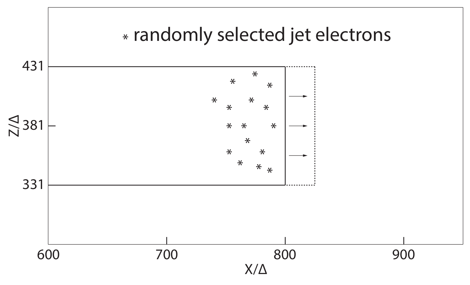
Figure 1: Schematic representation of the frontal jet volume, from where the electrons are selected when performing calculations of the radiation spectra. During the spectra calculations, the jet head moves 25 grid cells, from $x=800\Delta$ to $x=825\Delta$. We trace jet electrons that have a Lorentz factor of $\gamma>12$ and $\gamma>80$ for a plasma jet moving with a bulk Lorentz factor of $\Gamma=15$ and $\Gamma=100$, respectively.

3 Results and interpretation

In this section, we study the spectra from a top-hat nonthermal distribution of particles moving in the electromagnetic fields modified by kinetic instabilities in the presence of an initial toroidal magnetic field.

3.1 Global system evolution and electron acceleration

We note that $t=700\,\omega_{\rm pe}^{-1}$ corresponds to a time of the simulation which is deep into the non-linear regime of the growing instabilities (see Meli et al. (2023)). To obtain a radiation spectrum from PIC simulations at a given time $t$ (see Subsect. 3.3.3 below), we have to trace the jet electrons over a time interval around $t$ with a high temporal resolution $\Delta t_{\rm s}$. It is near to impossible to trace all jet electrons and, therefore, we select (or sample) a feasible number of electrons. Once we sample the positions, the velocities, and the accelerations of the jet electrons, we can then calculate the radiation spectra using Eq. (3).

We randomly select jet electrons from a region located behind the jet head, as shown by the small stars in Fig. 1, to calculate the resulting spectra. During the spectra calculations, the jet head moves 25 grid cells, from $x=800\Delta$ to $x=825\Delta$.

Depending on the setup of the plasma species (e^± or e^-- i⁺) in the jet, we select electrons with a Lorentz factor $\gamma>12$ for a jet with $\Gamma=15$ and with $\gamma>80$ for a jet with $\Gamma=100$, and starting from $t\gtrsim 700\omega_{pe}^{-1}$ we trace them for 5,000 steps with a time-step $\Delta t_{\rm s}=0.005\,\omega_{\rm pe}^{-1}$, thus the jet head moves over 25 grid cells, within a time interval of $t_{\rm s}=25\,\omega_{\rm pe}^{-1}$. This time-step used for calculating spectra is 200 times smaller than that utilized in the case of the main PIC plasma simulations, $\Delta t=0.1\,\omega_{\rm pe}^{-1}$, as it is also set in the simulations performed by Meli et al. (2023). When tracing the particles, we iterate 10 times over calculating the positions and the velocities of the particles. The Nyquist frequency is at $\omega_{\rm N}=1/(2*0.005*0.1)\,\omega_{\rm pe}=10^{3}\,\omega_{\rm pe}$, where the factor 0.1 in denominator accounts for the fact that we iterate 10 times over when calculating the positions and the velocities of the particles, for each time step of the simulations while performing spectra calculations, which is $\Delta t_{\rm s}=0.005\,\omega_{\rm pe}^{-1}$. The frequency resolution is $\Delta\omega=1/t_{\rm s}=0.04\,\omega_{\rm pe}$, which is small enough to provide smooth spectra.

e^± jet with $\mathbf{\Gamma=15}$ (a) e^-- i⁺ jet with $\mathbf{\Gamma=15}$ (b)

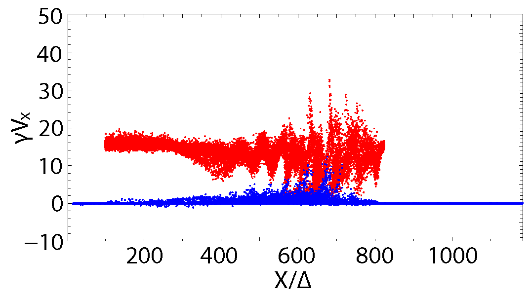
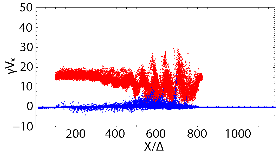
e^± jet with $\mathbf{\Gamma=100}$ (c) e^-- i⁺ jet with $\mathbf{\Gamma=100}$ (d)

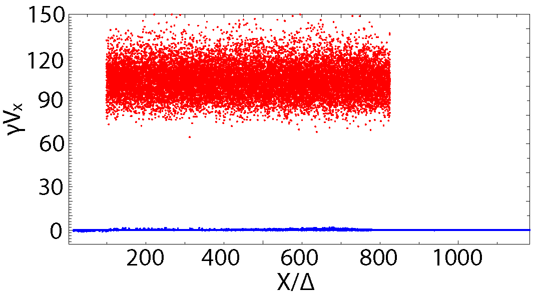
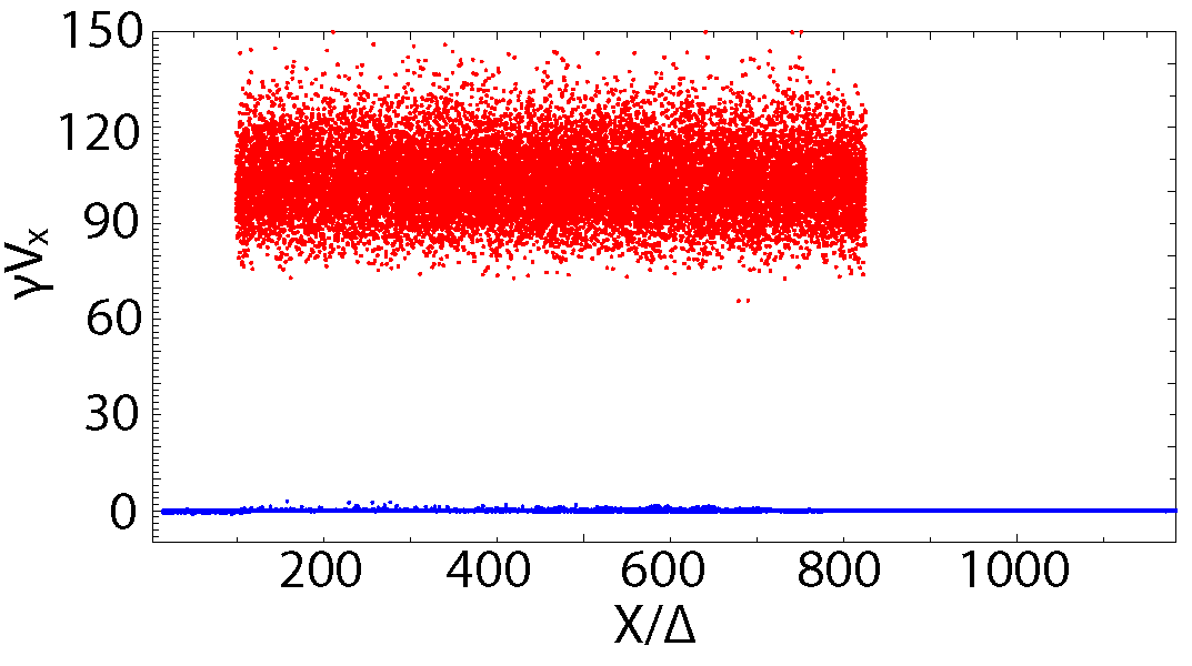
Figure 2: $x$ - $\gamma v_{x}$ distribution of jet (red) and ambient (blue) electrons for an e^± jet (left panels) and for an e^-- i⁺ jet (right panels) with $B_{0}=0.5$, at $t=725\omega^{-1}_{\rm pe}$. Upper panels correspond to jets with a jet Lorentz factor of $\Gamma=15$, while lower panels are for jets with $\Gamma=100$.

e^± jet with $\mathbf{\Gamma=15}$ (a) e^-- i⁺ jet with $\mathbf{\Gamma=15}$ (b)

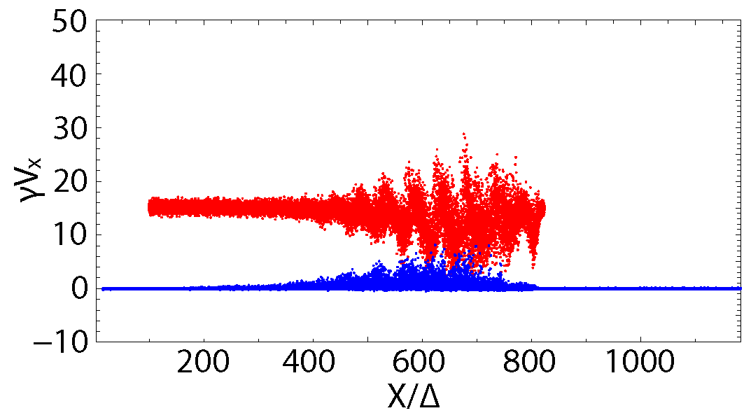
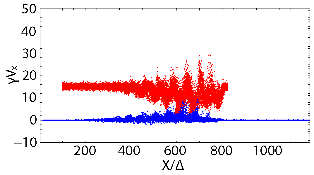
e^± jet with $\mathbf{\Gamma=100}$ (c) e^-- i⁺ jet with $\mathbf{\Gamma=100}$ (d)

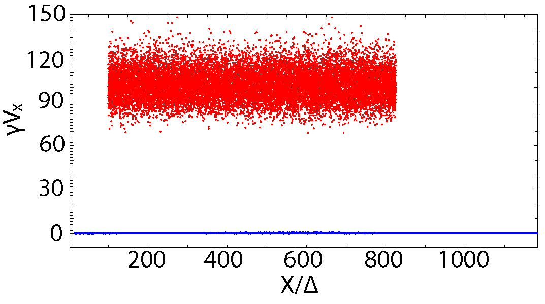
Figure 3: $x$ - $\gamma v_{x}$ distribution of jet (red) and ambient (blue) electrons for an e^± jet (left panels) and for an e^-- i⁺ jet (right panels) with $B_{0}=0.1$, at $t=725\omega^{-1}_{\rm pe}$. Upper panels correspond to jets with a bulk Lorentz factor of $\Gamma=15$, while lower panels are for jets with $\Gamma=100$.

e^± jet with $\mathbf{\Gamma=15}$               (a)                       e^-- i⁺ jet with $\mathbf{\Gamma=15}$               (b)

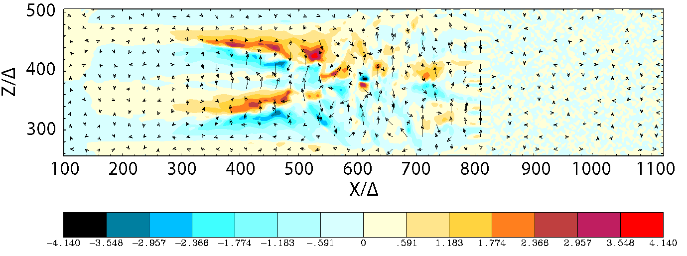
e^± jet with $\mathbf{\Gamma=100}$               (c)                       e^-- i⁺ jet with $\mathbf{\Gamma=100}$               (d)

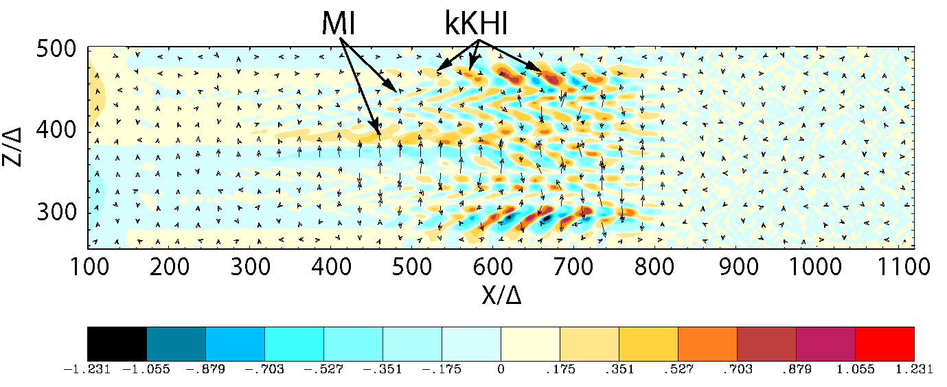
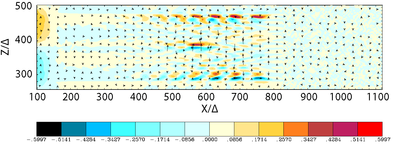
Figure 4: Distribution of the magnetic field in the $x-z$ plane of the simulation box, given for the case with $B_{0}=0.5$, at $t=725\,\omega^{-1}_{\rm pe}$. The left panels (a, c) are for an e^± jet, the right panels (b, d) are for an e^- - i⁺ jet. The upper panels (a, b) correspond to jets with a bulk Lorentz factor of $\Gamma=15$, the lower panels (c, d) are for jets with $\Gamma=100$. The out-of-plain $B_{y}$ component is shown with color maps, the in-plain field combined of $B_{x}$ and $B_{z}$ components is shown with arrows. The maximum and minimum are (a): $\pm 3.916$, (b): $\pm 4.140$, (c): $\pm 1.231$, and (d): $\pm 0.5997$.

e^± jet with $\mathbf{\Gamma=15}$               (a)                       e^-- i⁺ jet with $\mathbf{\Gamma=15}$               (b)

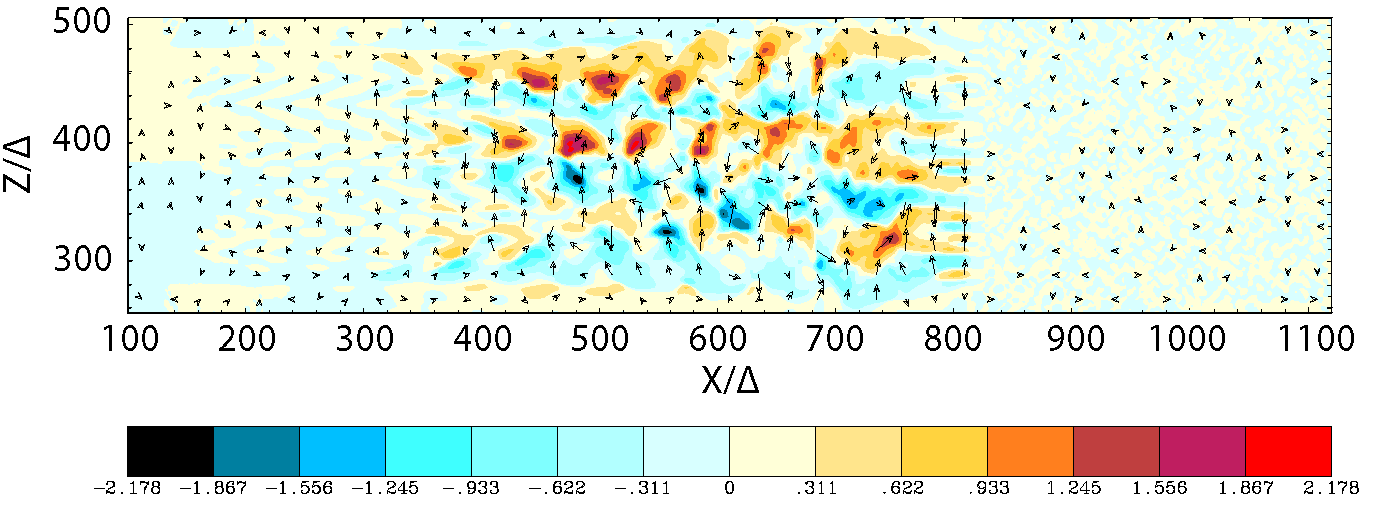
e^± jet with $\mathbf{\Gamma=100}$               (c)                       e^-- i⁺ jet with $\mathbf{\Gamma=100}$               (d)

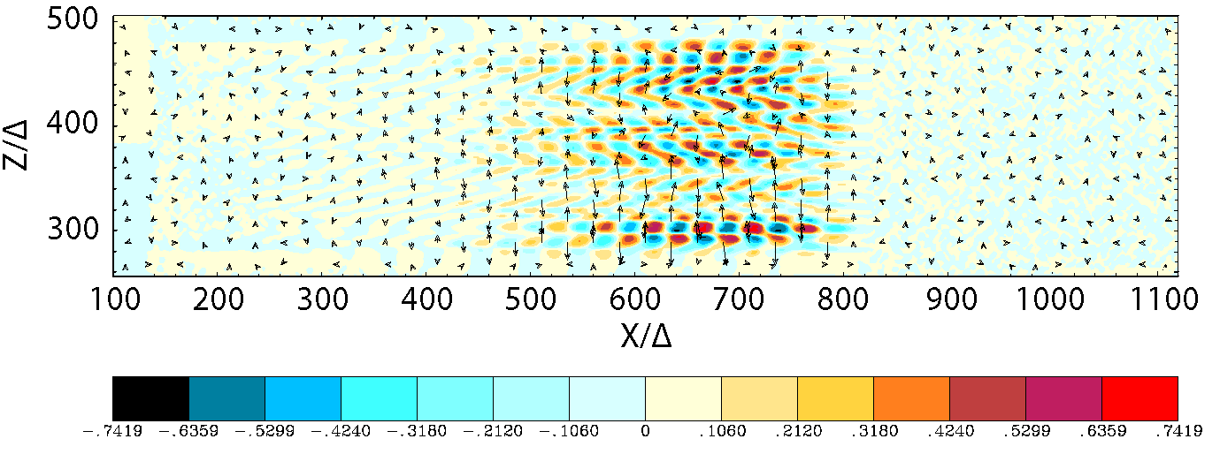
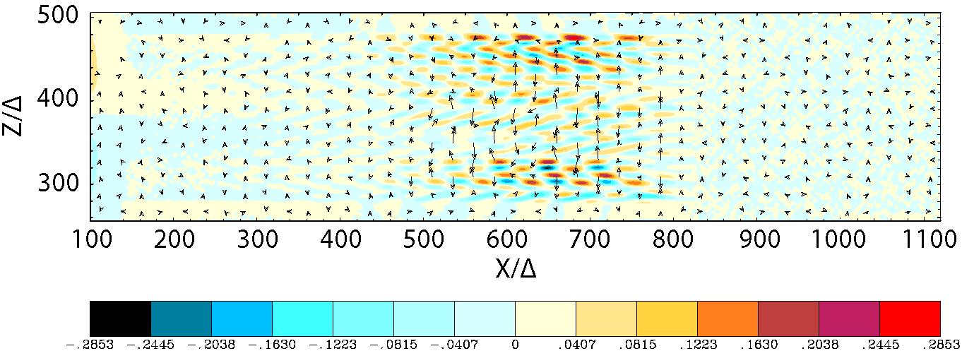
Figure 5: Distribution of the magnetic field in the $x-z$ plane of the simulation box, given for the case with $B_{0}=0.1$, at $t=725\,\omega^{-1}_{\rm pe}$. The left panels (a, c) are for an e^± jet, the right panels (b, d) are for an e^- - i⁺ jet. The upper panels (a, b) correspond to jets with a bulk Lorentz factor of $\Gamma=15$, the lower panels (c, d) are for jets with $\Gamma=100$. The out-of-plain $B_{y}$ component is shown with color maps, the in-plain field combined of $B_{x}$ and $B_{z}$ components is shown with arrows. The maximum and minimum are (a): $\pm 2.127$, (b): $\pm 2.178$, (c): $\pm 0.7419$, and (d): $\pm 0.2853$.

(a)                                             (b)                                             (c)

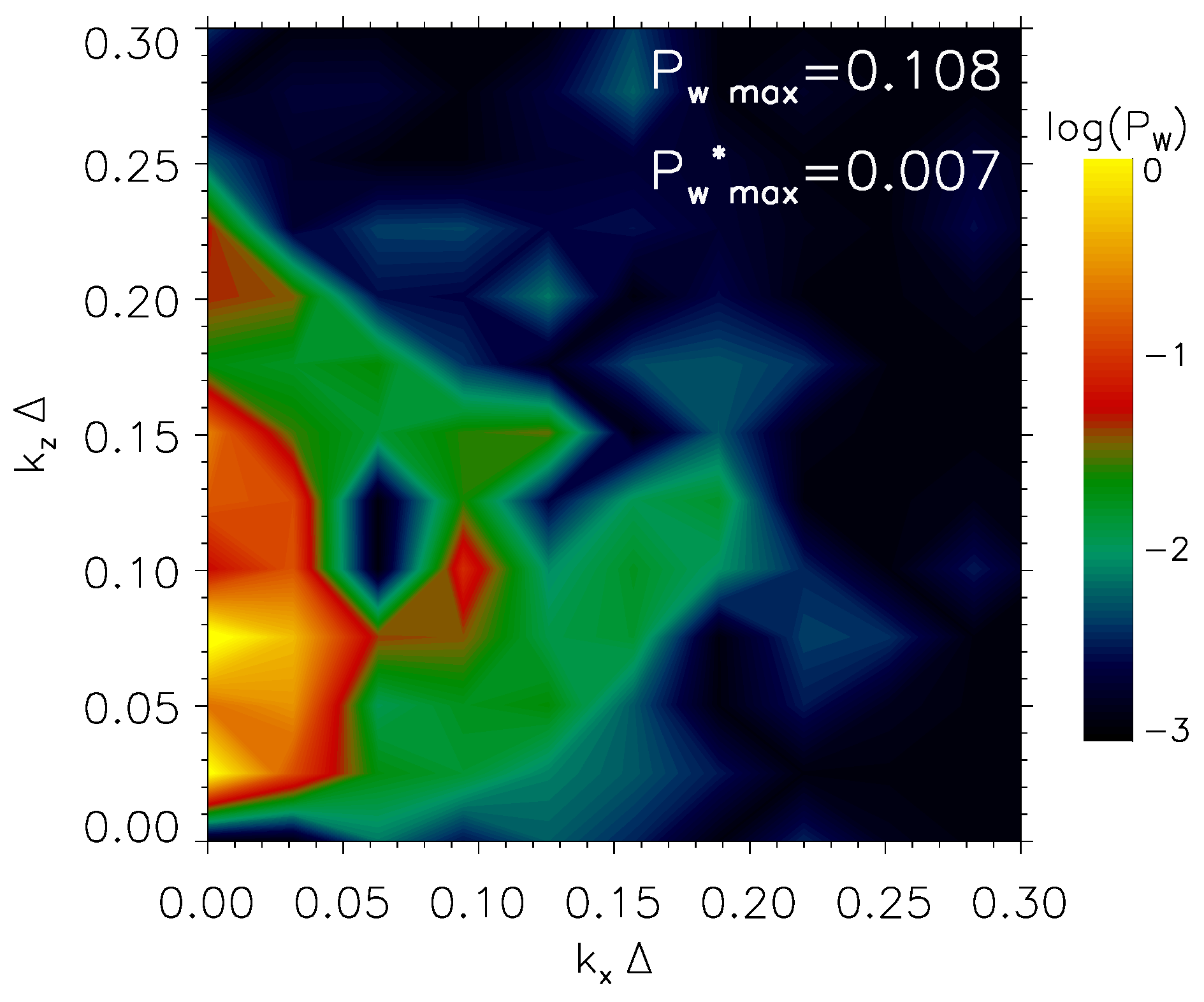
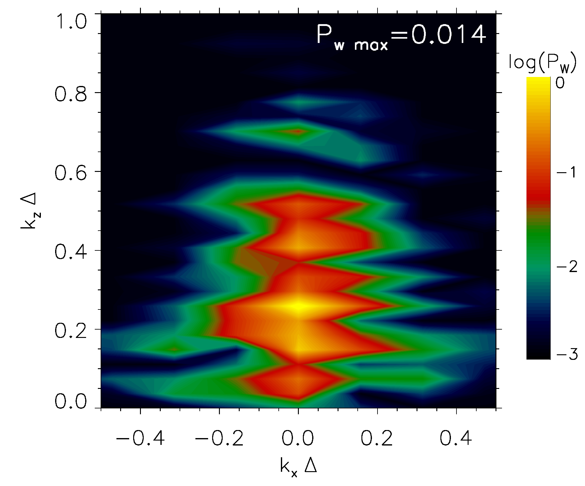
Figure 6: FFT-images of the magnetic field distribution ($B_{y}$ component) shown in Fig. 4(b) for the e^-- i⁺ jet with $\Gamma=15$ and $B_{0}=0.5$. The panels represent three regions: (a) $x\in[400-600]\,\Delta$, (b) $x\in[600-750]\,\Delta$ and (c) $x\in[780-820]\,\Delta$, which are also marked with white rectangles in Fig. 7. The color scale is logarithmic and normalized to the maximum wave power, so that numbers at the color bar mean $\rm{log}(P_{\rm{w}}/P_{\rm{w~{}max}})$. Corresponding values of $P_{\rm{w~{}max}}$ are given in right upper corners. $P^{~{}*}_{\rm{w~{}max}}=0.007$ in panel (a) corresponds to the local maximum at $(k_{x},\,k_{z})\,\Delta\approx(0.095,\,0.1)$.

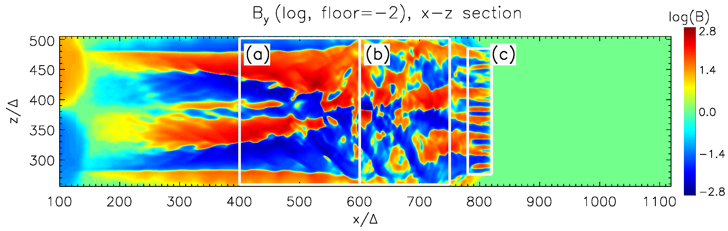
Figure 7: The same plot as Fig. 4(b), but with use of the sign-preserving logarithmic color scaling for $B_{y}$. We plot $\mathrm{sgn}(B_{y})\cdot\{2+\log[\max(|B_{y}|/B_{0},10^{-2})]\}$. The level of "0" on the color scale hence corresponds to $|B|/B_{0}\leq 10^{-2}$. The regions (a), (b) and (c) marked with white rectangles were used for FFT plots presented in Fig. 6.

The $x$ - $\gamma v_{x}$ distribution of the jet (red) and ambient (blue) electrons are shown for $B_{0}=0.5$ (in Fig. 2) and for $B_{0}=0.1$ (in Fig. 3) for an e^± and for an e^-- i⁺ jet (right panels) with initial jet Lorentz factors of $\Gamma=15$ and $\Gamma=100$. Although we do not calculate the spectra produced by the ambient electrons, we include here their phase-space ($x$ - $\gamma v_{x}$) representation just for comparison with the phase-space distribution of the electrons accelerated in the jet.

For a plasma jet with initial $\Gamma=15$, Figs. 2(a,b) and  3(a,b) show that the jet electrons (in red) are accelerated in bunches by growing instabilities; hence their momenta along the $x$-direction reach high values, where $\gamma{\rm v}_{x}$ doubles its value from $\gamma v_{x}\sim 15$ at injection, up to $\gamma v_{x}\sim 35$. On the contrary, for a plasma jet with initial $\Gamma=100$, the initial momentum of the jet electrons increases only by maximally 50$\%$ (Figs. 2(c,d) and  3(c,d)).

e^± jet with $\mathbf{\Gamma=15}$                 (a)                              e^-- i⁺ jet with $\mathbf{\Gamma=15}$           (b)

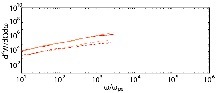
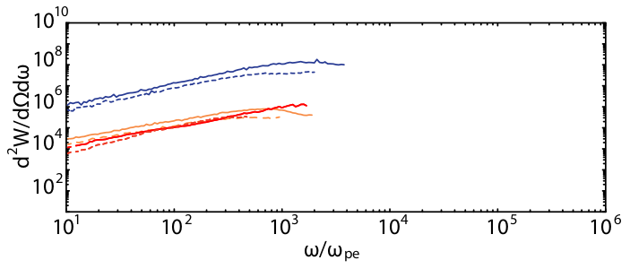
e^± jet with $\mathbf{\Gamma=100}$               (c)                              e^-- i⁺ jet with $\mathbf{\Gamma=100}$           (d)

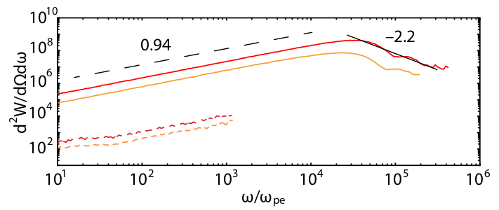
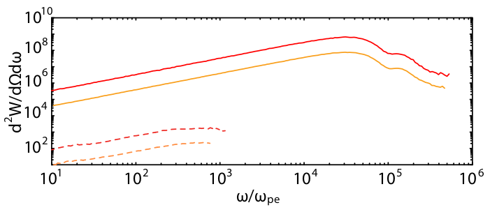
Figure 8: Synthetic spectra for e^± jets (left panels) and for e^-- i⁺ jets (right panels). Upper panels correspond to jets with a bulk Lorentz factor of $\Gamma=15$ (when selecting electrons with $\gamma>12$, except for the blue lines), while lower panels are for jets with $\Gamma=100$ (when selecting electrons with $\gamma>80$). The continuous line corresponds to the spectra for a head-on emission of jet electrons, whereas the dashed lines represent for 5^∘-off emission of radiation. The red lines show the cases with a stronger amplitude of the initial toroidal magnetic field, $B_{0}=0.5$, whereas the orange lines represent the spectra for $B_{0}=0.1$. In panel (b), the blue lines (solid for the head-on emission and dashed for the 5^∘-off emission) are obtained choosing jet electrons randomly including all Lorentz factors, whereas the dashed green lines show the slops of the selected case (blue solid line) and random case (red solid line), respectively. In panel (c), the slopes of the power-law segments at lower ($\sim 0.94$) and higher ($\sim-2.2$) frequency are indicated. The slopes for all spectra are listed in Table 1.

.

Panel	Emission	$B_{0}=0.5$ (red)	$B_{0}=0.1$ (orange)	$B_{0}=0.5$ (blue)
a) e±, $\Gamma=15$	head-on (solid)	$1.00\pm 0.01$	$0.95\pm 0.02$
	$5^{\circ}$-off (dashed)	$1.05\pm 0.01$	$0.93\pm 0.01$
b) e--i+, $\Gamma=15$	head-on (solid)	$0.97\pm 0.01$	$0.83\pm 0.01$	$0.84\pm 0.01$
	$5^{\circ}$-off (dashed)	$0.98\pm 0.03$	$0.77\pm 0.04$	$0.76\pm 0.01$
c) e±, $\Gamma=100$	head-on (solid)	$0.94\pm 0.003$	$0.98\pm 0.003$
		$\mathit{-2.22\pm 0.1}$	$\mathit{-1.55\pm 0.08}$
	$5^{\circ}$-off (dashed)	$0.84\pm 0.02$	$0.90\pm 0.01$
d) e--i+, $\Gamma=100$	head-on (solid)	$0.87\pm 0.01$	$0.91\pm 0.01$
		$\mathit{-2.26\pm 0.10}$	$\mathit{-2.46\pm 0.13}$
	$5^{\circ}$-off (dashed)	$0.91\pm 0.01$	$0.92\pm 0.01$

Table 1: Slopes of the spectra presented in Fig. 8. The four values in italic are the slopes of the decreasing legs of the solid curves (head-on) in panels c) and d).

In Fig. 4(a), around $x\sim 400\Delta$, we observed that the growth of MI is stronger, which in the $x-z$ plane can be seen as two pairs of layers, with opposite polarity of the magnetic field (these layers are actually the projection onto the $x-z$ plane of the circularly clockwise - as seen from the head of the jet - $B_{\phi}$ component of the magnetic field generated by the MI). At about $x\sim 500\Delta$, the magnetic field generated by MI is modulated by the kKHI, which later on dominates over the MI (as its growth time is longer than that of MI). Then, the nonlinear regime of plasma instabilities is reached, and the magnetic fields starts to dissipate. This is the stage of the plasma magnetic field when we begin to select jet electrons to calculate spectra. In Fig. 4(b), the instabilities grow in a similar way as in the case in Fig. 4(a), except that the kKHI is more visible.

For a weaker amplitude of the initial toroidal magnetic field (i) in Figs. 5(a,c,d) the dominant growing mode of kinetic instabilities is the WI, depicted as oblate stripes, which is different from the cases in Figs. 4(a,c,d), where the modes of MI and kKHI are dominant and (ii) in Fig. 5(b), the kKHI and MI are more visible than in Figs. 5(a,c,d).

3.2 Analysis of turbulence

We use the Fast Fourier Transform (FFT) to convert the amplitude of the $B_{y}$ wave components of the magnetic field shown in Fig. 4(b) from the spatial domain to the wave vector domain (Fig. 6), in order to estimate the characteristic length-scale of the turbulence. We compute the power spectrum of the waves excited by kinetic plasma instabilities and represent it in colors, in log scale, in the ($k_{x}$, $k_{z}$) wave vector space, where the wave vectors are defined as $|\vec{k}|\equiv 2\pi/\lambda$.

The space regions selected for FFT plots are shown in Figure 7. It represents the same distribution of $B_{y}$ as in Fig. 4(b), but plotted in logarithmic color scale, in order to resolve weaker field amplitudes together with stronger ones. Such an approach helps us to make the proper choice of the regions for analysis. These regions are marked in Fig. 7 with white rectangles: (a) for $x\in[400-600]\,\Delta$, (b) for $x\in[600-750]\,\Delta$ and (c) for $x\in[780-820]\,\Delta$. The selection has been made in a way to avoid the mixture of different waves in the same region, to make the FFT plots cleaner and easier for interpretation.

Region (a). The strongest modes observed in Fig. 6(a) are perpendicular to the jet axis ($k_{x}\,\Delta=0$) and have two maxima at $k_{z}\,\Delta=0.025\pm 0.007$ and $k_{z}\,\Delta=0.075\pm 0.007$. The corresponding wavelengths $\lambda=(250\pm 70)\,\Delta$ and $\lambda=(84\pm 8)\,\Delta$ are related rather to the global radial structure of the jet than to the turbulence. At the same time, there is a weaker oblique mode at $(k_{x},\,k_{z})\,\Delta=(0.095\pm 0.009,\,0.100\pm 0.007)$, with corresponding wavelength $\lambda_{\rm{obl}}=2\pi/\sqrt{k_{x}^{2}+k_{z}^{2}}=(45\pm 4)\,\Delta$ and relative wave power $P_{\rm w}\approx 0.007$. The later is associated with turbulent structure in this region with obliquity $\theta\approx 45^{\circ}$.

Region (b). This region is evidently most turbulent among all selected (see Fig. 7). Correspondingly, a mixture of various wave modes in this region is observed in the FFT plot in Fig. 6(b). The dominating modes are two perpendicular with $k_{z}\,\Delta=0.028\pm 0.007$ and $k_{z}\,\Delta=0.080\pm 0.007$, as well as one oblique with $(k_{x},\,k_{z})\,\Delta=(0.085\pm 0.012,\,0.082\pm 0.007)$. The corresponding wavelengths are $\lambda=(250\pm 70)\,\Delta$, $\lambda=(79\pm 7)\,\Delta$ and $\lambda=(53\pm 6)\,\Delta$, in the same sequence. The first one, like in the case of region (a), reflects the global system symmetry and it is not related to the turbulence. Meanwhile, two other with $\lambda_{\perp}\approx 79\,\Delta$ and $\lambda_{\rm{obl}}\approx 53\,\Delta$ ($\theta\approx 45^{\circ}$) are obviously related to the strong magnetic turbulence observed in this region and have comparable wave power $P_{\rm w}\approx 0.015$.

Region (c) is relatively thin and corresponds to the front of the jet. The series of wave modes observed here are strictly perpendicular to the jet axis and can be associated with turbulence due to the mixing of plasma populations in the nonlinear regime. In Fig. 6(c) they are presented with a set of maxima at $k_{x}\,\Delta=0$. The strongest one has $k_{z}\,\Delta=0.26\pm 0.01$ corresponding to a wavelength of $\lambda_{\perp}=(24\pm 1)\,\Delta$ with relative wave power $P_{\rm w}\approx 0.014$. Other maxima are several times weaker.

We note that, in our simulations, the electron skin depth is $\lambda_{\rm e}=10\,\Delta$, therefore the wavelength of the strongest wave mode becomes $\lambda_{\perp}=(2.4\pm 0.1)\,\lambda_{\rm e}$. For comparison, in the theory of the jitter radiation (e.g., Medvedev & Loeb, 1999; Medvedev, 2000), the characteristic coherence scale of the generated magnetic field by the relativistic generalization of the two-stream WI in an electron-ion plasma is of the order of the relativistic skin depth, $\sim\lambda_{\rm e}$. Furthermore, the front region where $x\in[600-800]\,\Delta$ might correspond, based on an educated guess, to the jet region from where we trace the electrons for calculating the spectra of jitter-like radiation (see the next subsection).

3.3 Synthetic spectra calculation

First, we calculate the radiation spectra for an initial toroidal magnetic field of moderate strength, $B_{0}=0.5$ (see Eqs. 1-2), which corresponds to a plasma magnetization of $\sigma=1.73\times 10^{-2}$. This setup of the initial toroidal magnetic field is also the case for the studies of plasma instabilities and particle acceleration by Meli et al. (2023).

Here, we analyze the impact of the strength of the initial helical magnetic field on the emission of radiation from the jet electrons for the two types of plasma used to model the jet. In Fig. 8, we represent the spectra of the radiated power $P(\omega)=d^{2}W/d\Omega d\omega$ as a function of the emitted frequencies, $\omega/\omega_{\rm pe}$, for a moderate, $B_{0}=0.5$, initial toroidal magnetic field (red lines) and for a weaker field of $B_{0}=0.1$ (orange lines), for two viewing angles: head-on emission of jet electrons (solid lines) and for 5^∘-off emission (dashed lines).

For an $e^{\pm}$ jet with $\Gamma=15$ (Fig. 8(a)), we cut the spectra at about $10^{3}\,\omega/\omega_{\rm pe}$, slightly beyond the Nyquist frequency. However, in the case of $e^{-}-i^{+}$ jets with the same $\Gamma=15$ (Fig. 8(b)), the spectra show a peak in frequency, even at a higher frequency ($10^{4}\,\omega/\omega_{\rm pe}$), the location of which depends on how the jet electrons are accelerated by the magnetic (and electric) fields modified from their initial setup by kinetic instabilities. This fact is reflected through the color maps of $B_{y}$, where in Fig 4(b) for $B_{0}=0.5$, the amplified magnetic field ($B_{y}^{\max}=\pm 4.14$) is stronger than for the case of $B_{0}=0.1$ ($B_{y}^{\max}=\pm 2.178$ in Fig 5(b)), and therefore the jet electrons are much more accelerated in the former case. (We can also observe the difference in particle acceleration by comparing Fig 2(b) and Fig 3(b).)

We have also performed spectra calculation for positrons in the case of an $e^{\pm}$ plasma jet (not shown here). Their spectral characteristics are similar to those for radiation emitted by electrons. Therefore, a factor of two should be added to the emission power to account for both electron and positron emission.

For a jet with $\Gamma=100$ (Figs. 8(c,d)), the peak frequency of the spectra is shifted to higher frequencies ($\sim 3\times 10^{4}\,\omega/\omega_{\rm pe}$) than in the cases of $\Gamma=15$, for both plasma compositions. Since in this case the bulk Lorentz factor is $\sim 6.7$ higher, the jet electrons are swerved, producing spectra with higher frequency beyond the Nyquist frequency. We note that the emission powers for a 5^∘ angle (dashed lines) is by two order of magnitude weaker than that for head-on emission, for a jet with $\Gamma=100$ (Figs. 8(c,d)). For $\Gamma=15$ (Figs. 8(a,b)), at the two observing angles the spectra are not that much separated. Moreover, these spectra are questionable beyond the Nyquist frequency.

The radiation power shows similar values in both cases of $e^{\pm}$ and $e^{-}-i^{+}$ jets with $\Gamma=100$ (Fig. 8(c,d)) since there is not too much difference between the particle species (positrons versus ions with a mass ratio of 4). For a head-on emission from a $e^{\pm}$ jet with $\Gamma=100$ (red lines in Fig. 8(c)), the observed difference in the amplitude of the radiation power results from different values of the generated magnetic field, the maximum of which is $B_{y}^{\max}=\pm 1.231$ (Fig. 4(c)) versus $B_{y}^{\max}=\pm 0.741$ (Fig. 5(c)). For a jet with $\Gamma=15$, the spectra for head-on and 5^∘-off emission have similar powers, more specifically in the case for an e^-- i⁺ plasma, whereas for a jet with $\Gamma=100$, the emission power is more than two orders of magnitude stronger for head-on emission than for 5^∘-off emission. This discrepancy arises from the fact that, in the case of a jet with $\Gamma=100$, the plasma instability excited in the transversal plane of the jet is very weak, therefore the electrons are less accelerated along the 5^∘-off direction and, as a consequence, the emitted power is very weak.

In Fig. 8(b), we represent with blue lines the spectra for head on (solid) and 5^∘-off (dashed) emission in the case of an $e^{-}-i^{+}$ jet with $\Gamma=15$ and $B_{0}=0.5$, when we do not impose a lower limit for the Lorentz factor of the electrons that we trace, thus the spectra are obtained by choosing jet electrons randomly including all values of their Lorentz factors. In this cases, both spectra for head-on and 5^∘-off emission present a peak, the amplitude of which is higher than the maximum amplitude that is observed in the spectra when we select electrons with $\gamma>12$, as the number of the particles that we trace in the former case are higher than that in the latter case.

In order to determine the slopes of all the spectra presented in Fig. 8, we performed a fit to power laws to each individual line (red, orange, blue; solid, dashed) based on the nonlinear least-squares (NLLS) Marquardt-Levenberg algorithm Levenberg (1944); Marquardt (1963). The resulting slopes, which are the exponents of the power laws, are summarized in Table 1; note that for $e^{\pm}$ and $e^{-}-i^{+}$ jets with $\Gamma=100$, the head-on spectra have an increasing and decreasing leg. For these cases, we have fitted both of them individually and state them separately in Table 1. In the low-frequency region of the spectra, we find that the power-law segment $\sim(\omega/\omega_{\rm pe})^{\alpha}$ has a slope $\alpha\sim 1$ for most cases, exception being for the $e^{-}-i^{+}$ jets with $\Gamma=15$ for two simulation setups (i) $B_{0}=0.1$ and $\gamma>12$ and (ii) $B_{0}=0.5$ and $\gamma$ randomly selected from all values, where the slope has a lower value, but still larger than that for the synchrotron radiation. The slopes for the $e^{-}-i^{+}$ jets with $\Gamma=15$ and $B_{0}=0.5$ decreases from $\sim 1$ to $\sim 0.8$ when randomly selecting electrons with all sorts of values of their Lorentz factor for both head-on and 5^∘-off emission. For jets with $\Gamma=100$ and for frequencies above the peak frequency, the spectra follows a power-law $\sim(\omega/\omega_{\rm pe})^{-\beta}$, where $\beta\sim 2.2$.

Our results show steeper spectra than those in the simulations performed by Sironi & Spitkovsky (2009), where the low-frequency part of the spectrum scales as $\omega^{1/3}$. The difference can arise from the fact that Sironi & Spitkovsky (2009) calculate the spectra from particles accelerated in relativistic collisionless shocks triggered by reflecting an incoming cold upstream flow, where the magnetic fields are generated by the WI. Instead, in the current work the spectra are calculated for the electrons selected directly from simulations, whose initial energy distribution can differ. We have calculated the spectra self-consistently, as the magnetic fields and the accelerated particles, key ingredients for the radiation, are produced as part of the plasma evolution. Therefore, our approach looks to be more natural.

4 Discussions and conclusions

Using self-consistent, 3D PIC calculations, we have obtained the first synthetic spectra of jitter-like radiation emitted by electrons in relativistic jets containing an initial toroidal magnetic field.

We have injected a relativistic jet containing a toroidal magnetic field into an ambient plasma at rest and calculate spectra for two values of the bulk Lorentz factor: $\Gamma=15$ and $\Gamma=100$. (We have used the PIC code in the work by (Meli et al., 2023) and added subroutines for spectra calculation.) These values are typical for jets in AGN and GRB objects, respectively. Furthermore, we set up two values for the amplitude of the initially applied toroidal magnetic field ($B_{0}=0.5$ and $B_{0}=0.1$), in order to analyze the impact of the strength of the initial magnetic field on the characteristics of the calculated spectra.

To estimate the characteristic length-scale of the turbulence, we have used the FFT to convert the amplitude of the $B_{y}$ wave components of the magnetic field from the spatial domain to the wave vector domain. We have found that the strongest mode corresponds to a wavelength of $\lambda_{\perp}=(24\pm 1)\,\Delta=(2.4\pm 0.1)\,\lambda_{\rm e}$, where the electron plasma skin depth is $\lambda_{\rm e}=10\,\Delta$, in our simulations. For comparison, the jitter radiation is expected to emerge from relativistic particles traveling through small-scale, turbulent magnetic fields that are coherent on the scale of an electron plasma skin depth, where in the work by Medvedev (2000) the origin of the magnetic field comes from a relativistic version of the well-known two-stream WI in a plasma.

We have calculated synthetic spectra directly from self-consistent simulations in which growing kinetic instabilities (WI, kKHI, and MI) are developed simultaneously into a highly nonlinear regime of plasma for two types of particle species of the jet plasma (pair and electron-ion). The strength and structure of growing instabilities depend on many factors, such as the amplitude of the initial toroidal magnetic field, the bulk Lorentz factor of the jets, and the type of the jet plasma (see Figs. 4 and 5).

In recent years, several methods have been developed for calculating synthetic spectra using PIC simulations (e.g., Reville & Kirk, 2010; Kagan et al., 2016; Spisak et al., 2020; Zhang et al., 2023). Nevertheless, the closest results with which our synthetic spectra can be compered are in the papers by Sironi & Spitkovsky (2009) and, more recently, by Zhang et al. (2023).

On the one hand, in the paper by Sironi & Spitkovsky (2009), in the 3D case, the low-frequency part of the spectrum scales as $\omega^{1/3}$, which can be attributed to synchrotron radiation. In 2D, they calculate the spectra with artificially reduced intensity of the magnetic field and obtain a flatter slope as for a jitter-like radiation. Our results show jitter-like spectra with a steep slope, $\omega^{0.94}$, generated from jet electrons accelerated in a turbulent magnetic field, which resulted from growing instabilities (WI, kKHI, and MI), in the presence of an initial toroidal magnetic field, into the nonlinear regime.

On the other hand, Zhang et al. (2023) perform combined 2D PIC and polarized radiative transfer simulations to study synchrotron emission from magnetic turbulence in the blazar emission region. The calculated spectra are shown in the upper panel of Fig. 3, where a flatter slope can be observed when the turbulent magnetic field is weaker.

To explore applications of our results, and to offer another perspective at understanding the role of the physical conditions of jet plasma on the electron acceleration and emission processes, we qualitatively compare our simulations to observations of relativistic jets. PIC calculations are carried out in dimensionless grid units which must be scaled (via scaling factors) into physical units (i.e., cgs) (e.g., MacDonald & Nishikawa, 2021).

To rescale the radiation spectra obtained from simulations, we have to take into account the effects induced by (i) simulation time-scale (i.e., $\omega_{\rm pe}/\omega_{\rm pe}^{\rm sim}$) and (ii) relativistic Doppler shift ($\sim 2~{}\Gamma$), as the jet moves with a bulk Lorentz factor $\Gamma$ with respect to an observer at rest (Hededal, 2005).

Now, to rescale the time-scale of the simulations to the real space we divide all frequencies with the plasma frequency calculated in the simulation box, $\omega_{\rm pe}^{\rm sim}$, and multiplying them with the real $\omega_{\rm pe}$. From the simulation code, the electron plasma rest-frame frequency is calculated as $\omega_{\rm pe}^{\rm sim}=\sqrt{q_{\rm e}^{2}a_{\rm dens}/m_{\rm e}}$, where $q_{\rm e}=-0.01$, $a_{\rm dens}=12.0$, and $m_{\rm e}=0.12$. This means, $\omega_{\rm pe}^{\rm sim}=0.1\,\Delta_{\rm t}^{-1}$, where $\Delta_{\rm t}$ is the simulation unit time, which in our computations is set to unity.

The electron plasma rest-frame frequency in the jet is (in cgs units): $\omega_{\rm pe}=(4\pi e^{2}n_{\rm e}/m_{\rm e})^{1/2}=5.64\times 10^{4}\,(n_{\rm e}/\rm{cm}^{-3})^{1/2}$, where $n_{\rm e}$, $e$, and $m_{\rm e}$ denote the number density, charge, and mass of the electrons within the plasma. Next, we scale the PIC value of the number density to a fiducial value, which is estimated from observations, $n_{\rm e}=n_{\rm e}^{\rm obs}$. Such a value is not universal, being rather tailored to each jet in AGN or GRB objects. Here, we consider the case of the M87 jet, where the electron number density of the jet is $n_{\rm e}^{\rm M87}\lesssim 10^{4}$ cm^-3 (Kawashima et al., 2022), since the synchrotron flux from the jet should be less than the observed flux in M87 by Event Horizon Telescope observations (Event Horizon Telescope Collaboration, 2019). Therefore, $\omega_{\rm pe}\lesssim 5.64\times 10^{6}$ s^-1 and, the frequency range of spectra is $5.64\times 10^{7}$ s${}^{-1}\,-\,5.64\times 10^{10}$ s^-1 for relativistic jets with a similar jet density like M87 jet.

Thus, the spectra emitted by electrons in a jet (with $n_{\rm e}\sim n_{\rm e}^{\rm M87}$) that propagates with a bulk Lorentz factor of $\Gamma=15$ and $\Gamma=100$ should be shifted to higher frequencies by $\sim 5.64\times 10^{7}\cdot 2\cdot 15\simeq 1.7\times 10^{9}$ and $\sim 5.64\times 10^{7}\cdot 2\cdot 100\simeq 1.1\times 10^{10}$, respectively.

After applying the rescaling, the spectra for a $\Gamma=15$ jet with head-on emission peak in the infrared band (Fig. 8(a) and Fig. 8(b)). For a $\Gamma=100$ jet with head-on emission (Fig. 8(c) Fig. 8(d)), the spectra peak in the near-infrared area, and continue into the optical/UV band, following a power-law with slope $\omega^{-\beta}$.

Therefore, our calculations of spectra from jitter-like radiation can be a viable framework for the interpretation of some observations, namely the tera electron-volts (TeV) emission in some blazar/AGN jets and prompt and afterglow emission in some GRBs.

This is the first in a series of papers that aim to calculate synthetic spectra from PIC simulations of relativistic plasma jets, where the jets are injected into a very large simulation grid, where no periodic boundary conditions are applied in the direction of jet propagation. The present simulations are designed to trace electrons with a high Lorentz factor from a region located at the head of the jet, for a relatively short time (due to the very high computational costs). Different selection criteria for tracing the electrons and the use of the FFT analysis of turbulence for finding the strongest modes to localized the region from where to trace electrons will be address in following papers.

Further work should also exploit larger scale simulations, including cooling terms in the equation for the radiation power and an improved initial set-up (e.g., Gaussian jet density profile instead of the top-hat one, which is utilized in the work presented here, different plasma composition for the jet and for the ambient, more realistic mass ratios for ions or stronger initial magnetic fields), just to account for a more realistic description of the emission from relativistic jets. Larger simulation systems would also allow us to verify whether the magnetic field modified globally by kinetic instabilities (WI, kKHI, and MI) in the presence of an initial toroidal magnetic field can avoid dissipation and survive beyond a few hundred electron skin depths and to unveil the occurrence of plasma shocks by the presence of sharp variations in the magnetic field profiles. Thus, we should be able to calculate synthetic spectra in more specific and realistic jet conditions based on observations.

Data Availability

The data underlying this article will be shared on reasonable request to the corresponding author.

References

- Abdo et al. (2009) Abdo, A. A. et al. 2009, Science, 323, 1688
- Alves et al. (2012) Alves, E. P., Grismayer, T., Martin, S. F., et al. 2012, ApJ, 746, L14
- Blandford et al. (2019) Blandford, R., Meier, D., & Readhead, A. 2019, Annual Review of Astronomy and Astrophysics, 57, 467
- Boris (1970) Boris, J. P. 1970, Proceeding of Fourth Conference on Numerical Simulations of Plasmas, p. 3-67
- Buneman (1993) Buneman, O. 1993, in Computer Space Plasma Physics: Simulation Techniques and Software; Eds: Matsumoto, H., Omura, Y., Terra Scientific Publishing Company: Tokio, Japan, p. 67-79
- Event Horizon Telescope Collaboration (2019) Event Horizon Telescope Collaboration 2019, ApJ, 875, L5
- Frederiksen et al. (2010) Frederiksen, J. T., Haugbolle, T., Medvedev, M. V., & Nordlund, Å. 2010, ApJ, 722, L114
- Gabuzda (2017) Gabuzda, D. 2017, Galaxies, 5, 11
- Ghirlanda et al. (2019) Ghirlanda, G., Salafia, O. S., Paragi, Z., et al. 2019, Science, 363, 968
- Hededal (2005) Hededal, C.B. 2005, Ph.D. thesis, arXiv:astro-ph/0506559
- Jackson (1999) Jackson, J. D. 1999, Classical Electrodynamics, (Interscience, Boston)
- Kagan et al. (2016) Kagan, D., Nakar, E., & Piran, T. 2016, ApJ, 826, 221
- Kawashima et al. (2022) Kawashima, T., Ishiguro, S., Moritaka, T., et al. 2022, ApJ, 928, 10
- Levenberg (1944) Levenberg, K. 1944, Quart. Appl. Math., 2, 164–168
- Lister et al. (2009) Lister, M. L., Cohen, M. H., Homan, D. C., et al. 2009, 138, 1874
- Lobanov & Zensus (2001) Lobanov, A. P. & Zensus, J. A. 2001, Science, 294, 128
- MacDonald & Nishikawa (2021) MacDonald, N. R. & Nishikawa, K.-I. 2021, A&A, 653, 19
- Marquardt (1963) Marquardt, D.W. 1963, J. Soc. Indust. Appl. Math., 11, 431–441
- Medvedev (2000) Medvedev, M. V. 2000, ApJ 540, 704
- Medvedev & Loeb (1999) Medvedev, M. V. & Loeb, A. 1999, ApJ 526, 697
- Meli et al. (2023) Meli A., Nishikawa, K.-I., Köhn, C. et al. 2023, MNRAS, 519, 5410
- Meszaros & Rees (2014) Meszaros, P. & Rees, M. J. 2014, in General Relativity and Gravitation: A Centennial Perspective, Eds: A. Ashtekar, B. Berger, J. Isenberg and M.A.H. MacCallum, Cambridge University Press, p. 148 (also arXiv:1401.3012)
- Mizuno et al. (2015) Mizuno, Y., Gómez, J. L., Nishikawa, K.-I., et al. 2015, ApJ, 809, 38
- Niemiec et al. (2008) Niemiec, J., Pohl, M., Stroman, T., & Nishikawa, K.-I. 2008, ApJ, 684, 1174
- Nishikawa et al. (2021) Nishikawa, K.-I., Duţan, I., Köhn, C., and Mizuno, Y., 2021, Living Reviews in Computational Astrophysics, 7, 1
- Nishikawa et al. (2016b) Nishikawa, K.-I., Mizuno, Y., Niemiec, J., et al. 2016b, Galaxies, 4, 38
- Nishikawa et al. (2016a) Nishikawa, K.-I., Frederiksen, J. T., Nordlund, Å., et al. 2016a, ApJ, 820, 94
- Nishikawa et al. (2014) Nishikawa, K.-I., Hardee, P. E., Duţan, I., et al. 2014, ApJ, 793, 60
- Nishikawa et al. (2013b) Nishikawa, K. -I., Hardee, P., Mizuno, Y., et al. 2013b, EPJ Web of Conferences, 61, 02003
- Nishikawa et al. (2013a) Nishikawa, K.-I., Hardee, P. E., Zhang, B., et al. 2013a, Ann. Geophys., 31, 1535
- Nishikawa et al. (2012) Nishikawa, K.-I., Zhang, B., Choi, E. J., et al. 2012, Procs. of the IAU, Vol. 279, p. 371-372
- Nishikawa et al. (2011) Nishikawa, K.-I., Niemiec, J., Medvedev, M., et al. 2011, AIP Conf. Proc. 1366, 163
- Nishikawa et al. (2009b) Nishikawa, K.-I., Medvedev, M., Zhang, B., et al. 2009, AIP Conference Proceedings, Volume 1133, pp. 235-237
- Nishikawa et al. (2009a) Nishikawa, K.-I., Niemiec, J., Hardee, P. E., et al. 2009b, ApJ, 698, 10L
- Nishikawa et al. (2008) Nishikawa K.-I., Niemiec, J., Sol, H., et al. 2008, AIP Conference Proceedings, 1085, 589
- Nishikawa et al. (2005) Nishikawa, K.-I., Hardee, P. E., Richardson, G., et al. 2005, ApJ, 622, 927
- Nishikawa et al. (2003) Nishikawa, K.-I., Hardee, P. E., Richardson, G., et al. 2003, ApJ, 595, 555
- Pasetto et al. (2021) Pasetto, A., Carrasco-González, C., Gómez, J. L., et al. 2021, ApJ, 923, L5
- Reville & Kirk (2010) Reville, B. & Kirk, J. G. 2010, ApJ, 724, 1283
- Rybicki & Lightman (1979) Rybicki, G. B., & Lightman, A. P. 1979, Radiative Processes in Astrophysics, (John Wiley & Sons, New York)
- Saikia et al. (2019) Saikia, P., Russell, D. M., Bramich, D.M., & Miller-Jones, J. C. A 2019, ApJ, 887, 21
- Sironi & Spitkovsky (2009) Sironi, L. & Spitkovsky, A. 2009, ApJ, 707, L92
- Spisak et al. (2020) Spisak, J., Liang, E., Fu, W., & Boettcher, M. 2020, ApJ, 903, 120
- Zhang et al. (2023) Zhang, H., Marscher, A. P., Guo, F., et al. 2023, ApJ, 949, 71