Lyapunov-Based Deep Residual Neural Network (ResNet) Adaptive Control

Abstract

Deep Neural Network (DNN)-based controllers have emerged as a tool to compensate for unstructured uncertainties in nonlinear dynamical systems. A recent breakthrough in the adaptive control literature provides a Lyapunov-based approach to derive weight adaptation laws for each layer of a fully-connected feedforward DNN-based adaptive controller. However, deriving weight adaptation laws from a Lyapunov-based analysis remains an open problem for deep residual neural networks (ResNets). This paper provides the first result on Lyapunov-derived weight adaptation for a ResNet-based adaptive controller. A nonsmooth Lyapunov-based analysis is provided to guarantee asymptotic tracking error convergence. Comparative Monte Carlo simulations are provided to demonstrate the performance of the developed ResNet-based adaptive controller. The ResNet-based adaptive controller shows a 64% improvement in the tracking and function approximation performance, in comparison to a fully-connected DNN-based adaptive controller.

I Introduction

Deep Neural Network (DNN)-based controllers have emerged as a tool to compensate for unstructured uncertainties in nonlinear dynamical systems. The success of DNN-based controllers is powered by the ability of a DNN to approximate any continuous function over a compact domain [1]. A popular DNN-based control method is to first perform a DNN-based offline system identification using sampled input-output datasets that are collected by conducting experiments [2, Sec. 6.6]. Then, using the identified DNN, a feedforward term is constructed to compensate for uncertainty in the system. However, the DNN weight estimates are not updated during task execution, and hence, such an approach involves static implementation of the DNN-based feedforward term. Since there is no continued learning with most DNN methods, questions arise regarding how well the training dataset matches the actual uncertainties in the system and the value or quality of the static feedforward model. This strategy motivates the desire for a large training dataset, but such data can be expensive or impossible to obtain, including the need for higher order derivatives that are typically not measurable.

Unlike offline methods, a closed-loop adaptive feedforward term can be developed by deriving real-time DNN weight adaptation laws from a Lyapunov-based stability analysis. Various classical results [3, 4, 5, 6, 7] use Lyapunov-based techniques to develop weight adaptation laws, but only for single-hidden-layer networks. These results do not provide weight adaptation laws for DNNs with more than one hidden layer, since there are mathematical challenges posed by the nested and nonlinear parameterization of a DNN that preclude the development of inner-layer weight adaptation laws. Recent results such as [8, 9, 10] develop Lyapunov-based adaptation laws for the output-layer weights of a DNN. However, to update the inner-layer weights, results in [8, 9, 10] collect datasets over discrete time-periods and iteratively identify the inner-layer weights using offline training algorithms. To circumvent offline identification of the inner-layer weights, the result in [11] provides a real-time inner-layer weight adaptation scheme based on a modular approach. However, modular designs only offer constraints on the adaptation laws and do not provide constructive insights on designing the adaptation laws.

Our recent work in [12] provides the first result on Lyapunov-derived weight adaptation laws for each layer of a DNN-based adaptive controller. To address the challenges posed by the nested and nonlinearly-parameterized structure of the DNN, a recursive representation of the DNN is developed. Then, a first-order Taylor series approximation is recursively applied for each layer. Using a Lyapunov-based stability analysis, the inner- and outer-layer weight adaptation laws are designed to cancel coupling terms that result from the approximation strategy. Although the result in [12] provides Lyapunov-derived weight adaptation laws for the DNN, the development is restricted to fully-connected DNNs.

There are several limitations associated with standard DNN architectures such as fully-connected and convolutional DNNs. Deeper networks typically suffer from the problem of vanishing or exploding gradients, i.e., the rate of learning using a gradient-based update rule is highly sensitive to the magnitude of DNN weights. Challenges faced from the vanishing or exploding gradient problem are ubiquitous to both offline training [13] and real-time weight adaptation [12]. Additionally, in applications such as image recognition, the performance of a DNN is found to initially improve by increasing the depth of the DNN. However, as the depth exceeds a threshold, performance rapidly degrades [14].

To overcome the vanishing or exploding gradient problem and the degradation of performance with the increasing depth of a DNN, results in [14] introduce shortcut connections across layers, i.e., a feedforward connection between layers that are separated by more than one layer. DNNs with a shortcut connection are known as deep residual neural networks (ResNets). Offline results in [15] and [16] offer mathematical explanations for why ResNets perform better than non-residual DNNs. In [15], the parameterization of a non-residual DNN is shown to cause difficulties in training DNN layers to approximate the identity function. As explained in [15], for a DNN to achieve a good training accuracy, the DNN layers must be able to approximate the identity function well. Since a shortcut connection in ResNets is represented using an identity function, ResNets provide an improved performance when compared to non-residual DNNs. Additionally, the result in [16] provides explanations from Lyapunov stability theory on why ResNets are easier to train offline using the gradient descent algorithm as compared to non-residual DNNs. The shortcut connections in ResNets facilitate the stability of the equilibria of gradient descent dynamics for a larger set of step sizes or initial weights as compared to non-residual DNNs.

Although there has been significant research across various applications involving ResNets [14, 17, 18, 19, 20], the approximation power of ResNets has not yet been explored for adaptive control problems. Developing a ResNet-based adaptive feedforward control term with real-time weight adaptation laws is an open problem. Although real-time weight adaptation laws are developed for fully-connected feedforward DNNs in [12], the shortcut connections in ResNets pose additional mathematical challenges. Unlike fully-connected DNNs, the shortcut connection prevents a recursive application of Taylor series approximation for each layer of the ResNet. As a result, it is difficult to generate the coupling terms that are generated using the approximation strategy in [12], that can be canceled using the weight adaptation laws in the Lyapunov-based analysis.

Our preliminary work in [21] and this paper provide the first result on Lyapunov-derived adaptation laws for the weights of each layer of a ResNet-based adaptive controller for uncertain nonlinear systems. To overcome the mathematical challenges posed by the residual network architecture, the ResNet is expressed as a composition of building blocks that involve a shortcut connection across a fully-connected DNN. Then, a constructive Lyapunov-based approach is provided to derive weight adaptation laws for the ResNet using the gradient of each DNN building block. A nonsmooth Lyapunov-based analysis is provided to guarantee asymptotic tracking error convergence. Unlike our preliminary work in [21], which involved a ResNet with only one shortcut connection, this paper provides weight adaptation laws for a general ResNet that has an arbitrary number of shortcut connections. The development of adaptation laws for ResNets with an arbitrary number of shortcut connections is challenging due to the complexity of the architecture. This challenge is addressed by constructing a recursive representation of the ResNet which involves a composition of an arbitrary number of building blocks. Then, based on the recursive representation of the ResNet architecture, a first-order Taylor series approximation is applied, which is then utilized to yield the Lyapunov-based adaptation laws. Additionally, unlike our preliminary work in [21] which did not provide simulations, this paper provides comparative Monte Carlo simulations to demonstrate the performance of the developed ResNet-based adaptive controller, and the results are compared with an equivalent fully-connected DNN-based adaptive controller [12]. Since the performance of ResNet and DNN-based adaptive controllers is sensitive to weight initialization, the Monte Carlo approach is used to provide a fair comparison between the two architectures. In the Monte Carlo comparison, 10,000 simulations are performed, where the initial weights in each simulation are selected from a uniform random distribution, and a cost function is evaluated for each simulation. Then, the simulation results yielding the least cost for both architectures are compared. The ResNet-based adaptive controller shows a 64% improvement in the tracking and function approximation performance, in comparison to a fully-connected DNN-based adaptive controller.

Notation and Preliminaries

The space of essentially bounded Lebesgue measurable functions is denoted by $\mathcal{L}_{\infty}$. The right-to-left matrix product operator is represented by $\stackrel{{\scriptstyle\curvearrowleft}}{{\prod}}$, i.e., $\stackrel{{\scriptstyle\curvearrowleft}}{{\stackrel{{\scriptstyle[}}{{p}}=1]{m}{\prod}}}A_{p}=A_{m}\ldots A_{2}A_{1}$ and $\stackrel{{\scriptstyle\curvearrowleft}}{{\stackrel{{\scriptstyle[}}{{p}}=a]{m}{\prod}}}A_{p}=I$ if $a>m$. The Kronecker product is denoted by $\otimes$. Function compositions are denoted using the symbol $\circ$, e.g., $(g\circ h)(x)=g(h(x))$, given suitable functions $g$ and $h$. The Filippov set-valued map defined in [22, Equation 2b] is denoted by $K\left[\cdot\right]$. The notation $\overset{a.a.t.}{(\cdot)}$ denotes that the relation $(\cdot)$ holds for almost all time (a.a.t.). Consider a Lebesgue measurable and locally essentially bounded function $h:\mathbb{R}^{n}\times\mathbb{R}_{\geq 0}\to\mathbb{R}^{n}$. Then, the function $y:\mathcal{I}\to\mathbb{R}^{n}$ is called a Filippov solution of $\dot{y}=h(y,t)$ on the interval $\mathcal{I}\subseteq\mathbb{R}_{\geq 0}$ if $y$ is absolutely continuous on $\mathcal{I}$ and $\dot{y}\overset{a.a.t.}{\in}K\left[h\right](y,t)$. Given $w\in\mathbb{R}$ and some functions $f$ and $g$, the notation $f(w)=\mathcal{O}^{m}(g(w))$ means that there exists some constants $M\in\mathbb{R}_{>0}$ and $w_{0}\in\mathbb{R}$ such that $\left\|f(w)\right\|\leq M\left\|g(w)\right\|^{m}$ for all $w\geq w_{0}$. Given some matrix $A\triangleq\left[a_{i,j}\right]\in\mathbb{R}^{n\times m}$, where $a_{i,j}$ denotes the element in the $i^{th}$ row and $j^{th}$ column of $A$, the vectorization operator is defined as $\mathrm{vec}(A)\triangleq[a_{1,1},\ldots,a_{1,m},\ldots,a_{n,1},\ldots,a_{n,m}]^{T}\in\mathbb{R}^{nm}$. The $p$-norm is denoted by $\left\|\cdot\right\|_{p}$, where the subscript is suppressed when $p=2$. The Frobenius norm is denoted by $\left\|\cdot\right\|_{F}\triangleq\left\|\mathrm{vec}(\cdot)\right\|$. Given any $A\in\mathbb{R}^{p\times a}$, $B\in\mathbb{R}^{a\times r}$, and $C\in\mathbb{R}^{r\times s}$, the vectorization operator satisfies the property [23, Proposition 7.1.9]

$$\mathrm{vec}(ABC) = (C^{T}\otimes A)\mathrm{vec}\left(B\right).$$ (1)

Differentiating (1) on both sides with respect to $\mathrm{vec}\left(B\right)$ yields the property

$$\frac{\partial}{\partial\mathrm{vec}\left(B\right)}\mathrm{vec}(ABC) = (C^{T}\otimes A).$$ (2)

II Unknown System Dynamics and Control Design

Consider a control-affine nonlinear dynamic system modeled as

$$\dot{x} = f(x)+u,$$ (3)

where $x:\mathbb{R}_{\geq 0}\rightarrow\mathbb{R}^{n}$ denotes a Filippov solution to (3), $f:\mathbb{R}^{n}\rightarrow\mathbb{R}^{n}$ denotes an unknown differentiable drift vector field, and $u:\mathbb{R}_{\geq 0}\rightarrow\mathbb{R}^{n}$ denotes a control input. Let the tracking error $e:\mathbb{R}_{\geq 0}\rightarrow\mathbb{R}^{n}$ be defined as

$$e \triangleq x-x_{d},$$ (4)

where $x_{d}:\mathbb{R}_{\geq 0}\rightarrow\mathbb{R}^{n}$ denotes a continuously differentiable reference trajectory. The reference trajectory is designed such that $\left\|x_{d}(t)\right\|\leq\overline{x_{d}}\;\forall t\in\mathbb{R}_{\geq 0}$ and $\dot{x}_{d}\in\mathcal{L}_{\infty},$ where $\overline{x_{d}}\in\mathbb{R}_{>0}$ is a constant. The control objective is to design a ResNet-based adaptive controller that achieves asymptotic tracking error convergence.

II-A ResNet Architecture

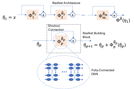
Figure 1: Illustration of the ResNet architecture in (6). The ResNet is shown at the top of the figure and is composed of building blocks that involve a shortcut connection across a fully-connected DNN component. The fully-connected DNN component for the $p^{th}$ building block (bottom) is denoted by $\Phi_{p}^{\theta_{p}}$ for all $p\in\{1,\ldots,m\}$, where the input and the vector of weights of $\Phi_{p}$ are denoted by $\eta_{p}$ and $\theta_{p}$, respectively. Then the output of the $p^{th}$ building block after considering the shortcut connection is represented by $\eta_{p+1}=\eta_{p}+\Phi_{p}^{\theta_{p}}(\eta_{p})$ for all $p\in\{1,\ldots,m-1\}$, and the output of the ResNet is $\eta_{m}+\Phi_{m}^{\theta_{m}}\left(\eta_{m}\right)$.

The unknown drift vector field $f$ can be approximated using a ResNet. A ResNet is modeled using building blocks that involve a shortcut connection across a fully-connected DNN [14]. Let $\Phi_{p}:\mathbb{R}^{L_{p,0}}\times\mathbb{R}^{L_{p,0}\times L_{p,1}}\times\ldots\times\mathbb{R}^{L_{p,k_{p}}\times L_{p,k_{p}+1}}\to\mathbb{R}^{L_{p,k_{p}+1}}$ denote the $p^{th}$ fully-connected DNN block defined as $\Phi_{p}(\eta_{p},V_{p,0},\ldots,V_{p,k_{p}})\triangleq\left(V_{p,k_{p}}^{T}\phi_{p,k_{p}}\circ...\circ V_{p,1}^{T}\phi_{p,1}\right)\left(V_{p,0}^{T}\eta_{p}\right)$ for all $p\in\{1,\ldots,m\}$, where $\eta_{p}\in\mathbb{R}^{L_{p,0}}$ denotes the input of $\Phi_{p}$, $k_{p}\in\mathbb{Z}_{>0}$ denotes the number of hidden layers in $\Phi_{p}$, and $m\in\mathbb{Z}_{>0}$ denotes the number of building blocks. Additionally, $L_{p,j}\in\mathbb{Z}_{>0}$ denotes the number of nodes, and $V_{p,j}\in\mathbb{R}^{L_{p,j}\times L_{p,j+1}}$ denotes the weight matrix in the $j^{th}$ layer of $\Phi_{p}$ for all $(p,j)\in\{1,\ldots,m\}\times\{0,\ldots,k_{p}\}$. Similarly, $\phi_{p,j}:\mathbb{R}^{L_{p,j}}\to\mathbb{R}^{L_{p,j}}$ denotes a vector of smooth activation functions. If the ResNet involves multiple types of activation functions at each layer, then $\phi_{p,j}$ may be represented as $\phi_{p,j}\triangleq\left[\varsigma_{p,j,1}\begin{array}[]{cc}\ldots&\varsigma_{p,j,L_{p,j}}\end{array}\right]^{T}$, where $\varsigma_{p,j,i}:\mathbb{R}\to\mathbb{R}$ denotes the activation function at the $i^{\mathrm{th}}$ node of the $j^{\mathrm{th}}$ layer of $\Phi_{p}$. All the weights of $\Phi_{p}$ can be represented by the vector $\theta_{p}\triangleq\left[\begin{array}[]{ccc}\mathrm{vec}(V_{p,0})^{T}&\ldots&\mathrm{vec}(V_{p,k_{p}})^{T}\end{array}\right]^{T}\in\mathbb{R}^{\Sigma_{j=0}^{k_{p}}L_{p,j}L_{p,j+1}}$. The fully-connected block $\Phi_{p}$ can be expressed as $\Phi_{p}=V_{p,k_{p}}^{T}\varphi_{p,k_{p}}$, where $\varphi_{p,0}:\mathbb{R}^{L_{p,0}}\to\mathbb{R}^{L_{p,0}}$ and $\varphi_{p,j}:\mathbb{R}^{L_{p,0}}\times\mathbb{R}^{L_{p,0}\times L_{p,1}}\times\ldots\times\mathbb{R}^{L_{p,j-1}\times L_{p,j}}\to\mathbb{R}^{L_{p,j}}$ $\forall j\in\{1,\ldots,k_{p}\}$ denote the recursive relation defined as

$$\varphi_{p,j} \triangleq \begin{cases}\phi_{p,j}\left(V_{p,j-1}^{T}\varphi_{p,j-1}\right),&j\in\left\{1,\ldots,k_{p}\right\},\\ \eta_{p},&j=0.\end{cases}$$ (5)

The arguments of $\varphi_{p,j}$ are suppressed for notational brevity. Let $\phi_{p,j}^{\prime}:\mathbb{R}^{L_{p,j}}\to\mathbb{R}^{L_{p,j}\times L_{p,j}}$ be defined as $\phi_{p,j}^{\prime}(y)\triangleq\frac{\partial}{\partial y}\phi_{p,j}(y)$ $\forall y\in\mathbb{R}^{L_{p,j}}$. The short-hand notation $\Phi_{p}^{\theta_{p}}(\eta_{p})\triangleq\Phi_{p}(\eta_{p},V_{p,0},V_{p,1},\ldots,V_{p,k_{p}})$ is defined for notational brevity in the subsequent development. Then the output of the $p^{th}$ building block is given by $\eta_{p}+\Phi_{p}^{\theta_{p}}(\eta_{p})$, where the addition of the input term $\eta_{p}$ represents the shortcut connection across $\Phi_{p}$. As shown in Figure 1, the ResNet $\Phi:\mathbb{R}^{n}\times\mathbb{R}^{\Sigma_{p=1}^{m}\Sigma_{j=0}^{k_{p}}L_{p,j}L_{p,j+1}}\to\mathbb{R}^{n}$, which defines the mapping $(\eta_{1},\theta)\mapsto\Phi^{\theta}\left(\eta_{1}\right)$, is modeled as [14]

$$\Phi^{\theta}\left(\eta_{1}\right) \triangleq \eta_{m}+\Phi_{m}^{\theta_{m}}\left(\eta_{m}\right),$$ (6)

where $\theta\triangleq\left[\begin{array}[]{ccc}\theta_{1}^{T}&\ldots&\theta_{m}^{T}\end{array}\right]^{T}\in\mathbb{R}^{\Sigma_{p=1}^{m}\Sigma_{j=0}^{k_{p}}L_{p,j}L_{p,j+1}}$ denotes the vector of weights for the entire ResNet, and $\eta_{m}$ is evaluated using the recursive relation

$$\eta_{p} = \begin{cases}\eta_{p-1}+\Phi_{p-1}^{\theta_{p-1}}\left(\eta_{p-1}\right),&p\in\{2,\ldots,m\},\\ x,&p=1.\end{cases}$$ (7)

The recursive relation in (7) has valid dimensions under the constraint $L_{1,0}=L_{1,k_{1}+1}=L_{2,0}=L_{2,k_{2}+1}=\ldots=L_{m,0}=L_{m,k_{m}+1}=n$. To facilitate the subsequent development, the following assumption is made.

Assumption 1.

The function space of ResNets given by (6) is dense in $\mathcal{C}(\Omega)$ with respect to the supremum norm, where $\mathcal{C}(\Omega)$ denotes the space of functions continuous over the compact set $\Omega\subset\mathbb{R}^{n}$.

Remark 1.

Assumption 1 implies that ResNets satisfy the universal function approximation property that is well-known for various DNN architectures [1]. The universal function approximation property of ResNets is a common assumption that is widely used in the deep learning literature, and has been rigorously established for ResNets with specific activation functions in [24] and [25].

Consider any vector field $f\in\mathcal{C}(\Omega)$ and a prescribed accuracy $\overline{\varepsilon}\in\mathbb{R}_{>0}$. Then by Assumption 1, there exists a ResNet $\Phi$ with sufficiently large $m,k_{p},L_{p,j}$ $\forall(p,j)\in\{1,\ldots,m\}\times\{0,\ldots,k_{p}\}$ and a corresponding vector of ideal weights $\theta^{*}\in\mathbb{R}^{\Sigma_{p=1}^{m}\Sigma_{j=0}^{k_{p}}L_{p,j}L_{p,j+1}}$ such that $\sup_{x\in\Omega}\left\|f(x)-\Phi^{\theta^{*}}(x)\right\|\leq\overline{\varepsilon}$. Therefore, the drift vector field $x\mapsto f(x)$ can be modeled as

$$f(x) = \Phi^{\theta^{*}}(x)+\varepsilon(x),$$ (8)

when $x\in\Omega$, where $\varepsilon:\mathbb{R}^{n}\rightarrow\mathbb{R}^{n}$ denotes an unknown function reconstruction error that can be bounded as $\sup_{x\in\Omega}\left\|\varepsilon(x)\right\|\leq\overline{\varepsilon}$.

To facilitate the subsequent analysis, the following assumption is made (cf., [26, Assumption 1]).

Assumption 2.

There exists a known constant $\overline{\theta}\in\mathbb{R}_{>0}$ such that the unknown ideal ResNet weights can be bounded as $\left\|\theta^{*}\right\|\leq\overline{\theta}$.

II-B Control and Adaptation Laws

The ResNet-based model in (8) can be leveraged to approximate the unknown drift vector field $f$. However, since the ideal weights are unknown, adaptive weight estimates are developed. The adaptive weight estimate for the $j^{th}$ layer of $\Phi_{p}$ is denoted by $\hat{V}_{p,j}:\mathbb{R}_{\geq 0}\rightarrow\mathbb{R}^{L_{p,j}\times L_{p,j+1}}$ $\forall(p,j)\in\{1,\ldots,m\}\times\{0,\ldots,k_{p}\}$. The weight estimate for the $p^{th}$ building block $\hat{\theta}_{p}:\mathbb{R}_{\geq 0}\rightarrow\mathbb{R}^{\Sigma_{j=0}^{k_{p}}L_{p,j}L_{p,j+1}}$ is defined as $\hat{\theta}_{p}=\left[\mathrm{vec}(\hat{V}_{p,0})^{T},\ldots,\mathrm{vec}(\hat{V}_{p,k_{p}})^{T}\right]^{T}$ for all $p\in\{1,\ldots,m\}$, the weight estimate for the ResNet $\hat{\theta}:\mathbb{R}_{\geq 0}\rightarrow\mathbb{R}^{\Sigma_{p=1}^{m}\Sigma_{j=0}^{k_{p}}L_{p,j}L_{p,j+1}}$ is defined as $\hat{\theta}\triangleq\left[\begin{array}[]{ccc}\hat{\theta}_{1}^{T}&\ldots&\hat{\theta}_{m}^{T}\end{array}\right]^{T}$, and the ResNet-based adaptive estimate of $f(x)$ $\forall x\in\Omega$ is denoted by $\Phi^{\hat{\theta}}(x)$. The weight estimation error $\tilde{\theta}:\mathbb{R}_{\geq 0}\rightarrow\mathbb{R}^{\Sigma_{p=1}^{m}\Sigma_{j=0}^{k_{p}}L_{p,j}L_{p,j+1}}$ is defined as $\tilde{\theta}\triangleq\theta^{*}-\hat{\theta}$. Based on the subsequent stability analysis, the adaptation law for the weight estimates of the ResNet in (6) is designed as

$$\dot{\hat{\theta}} \triangleq \Gamma\Phi^{\prime T}e,$$ (9)

where $\Gamma\in\mathbb{R}^{\Sigma_{p=1}^{m}\Sigma_{j=0}^{k_{p}}L_{p,j}L_{p,j+1}\times\Sigma_{p=1}^{m}\Sigma_{j=0}^{k_{p}}L_{p,j}L_{p,j+1}}$ denotes a positive-definite adaptation gain matrix, and $\Phi^{\prime}\in\mathbb{R}^{n\times\Sigma_{p=1}^{m}\Sigma_{j=0}^{k_{p}}L_{p,j}L_{p,j+1}}$ is a short-hand notation denoting the $\Phi^{\prime}\triangleq\frac{\partial\Phi^{\hat{\theta}}(x)}{\partial\hat{\theta}}$. The term $\Phi^{\prime}$ can be evaluated as follows. Let $\hat{\eta}_{p}\in\mathbb{R}^{L_{p,0}}$ be defined as

$$\hat{\eta}_{p}=\begin{cases}x,&p=1,\\ \hat{\eta}_{p-1}+\Phi_{p-1}^{\hat{\theta}_{p-1}}\left(\hat{\eta}_{p-1}\right),&p\in\{2,\ldots,m\}.\end{cases}$$ (10)

Then, it follows that $\Phi^{\hat{\theta}}\left(x\right)=\hat{\eta}_{m}+\Phi_{m}^{\hat{\theta}_{m}}(\hat{\eta}_{m})$. To facilitate the subsequent development, the short-hand notations $\Phi_{p}^{\prime}\triangleq\left(\frac{\partial\Phi^{\hat{\theta}}(x)}{\partial\hat{\theta}_{p}}\right)$, $\Lambda_{p}\triangleq\frac{\partial\Phi_{p}^{\hat{\theta}_{p}}\left(\hat{\eta}_{p}\right)}{\partial\hat{\theta}_{p}}$, $\Lambda_{p,j}\triangleq\frac{\partial\Phi_{p}^{\hat{\theta}_{p}}\left(\hat{\eta}_{p}\right)}{\partial\mathrm{vec}(\hat{V}_{p,j})}$, and $\Xi_{p}\triangleq\frac{\partial\Phi_{p}^{\hat{\theta}_{p}}\left(\hat{\eta}_{p}\right)}{\partial\hat{\eta}_{p}}$ are introduced. Then $\Phi^{\prime}=\left[\left(\frac{\partial\Phi^{\hat{\theta}}(x)}{\partial\hat{\theta}_{1}}\right),\ldots,\left(\frac{\partial\Phi^{\hat{\theta}}(x)}{\partial\hat{\theta}_{m}}\right)\right]$ can be expressed as

$$\Phi^{\prime} \triangleq \left[\begin{array}[]{ccc}\Phi_{1}^{\prime},&\ldots,&\Phi_{m}^{\prime}\end{array}\right].$$ (12)

Using the chain rule, the term $\Phi_{p}^{\prime}$ can be computed as

$$\Phi_{p}^{\prime}=\left(\stackrel{{\scriptstyle\curvearrowleft}}{{\stackrel{{\scriptstyle[}}{{l}}=p+1]{m}{\prod}}}\left(I_{n}+\Xi_{l}\right)\right)\Lambda_{p},\,\forall p\in\{1,\ldots,m\}.$$ (13)

In (13), the terms $\Lambda_{p}$ and $\Xi_{p}$, for all $p\in\{1,\ldots,m\}$, can be computed as follows. Since $\hat{\theta}_{p}=\left[\mathrm{vec}(\hat{V}_{p,0})^{T},\ldots,\mathrm{vec}(\hat{V}_{p,k_{p}})^{T}\right]^{T}$, it follows that $\frac{\partial\Phi_{p}^{\hat{\theta}_{p}}\left(\hat{\eta}_{p}\right)}{\partial\hat{\theta}_{p}}=\left[\left(\frac{\partial\Phi_{p}^{\hat{\theta}_{p}}\left(\hat{\eta}_{p}\right)}{\partial\mathrm{vec}(\hat{V}_{p,0})}\right),\ldots,\left(\frac{\partial\Phi_{p}^{\hat{\theta}_{p}}\left(\hat{\eta}_{p}\right)}{\partial\mathrm{vec}(\hat{V}_{p,k_{p}})}\right)\right]$. Therefore, using the definitions of $\Lambda_{p}$ and $\Lambda_{p,j}$ yields

$$\Lambda_{p}=\left[\begin{array}[]{cccc}\Lambda_{p,0}&\Lambda_{p,1}&\ldots&\Lambda_{p,k_{p}}\end{array}\right],\forall p\in\{1,\ldots,m\}.$$ (14)

For brevity in the subsequent development, the short-hand notations $\hat{\varphi}_{p,j}\triangleq\varphi_{p,j}(\hat{\eta}_{p},\hat{V}_{p,0},\ldots,\hat{V}_{p,j})$ and $\hat{\varphi}_{p,j}^{\prime}\triangleq\varphi_{p,j}^{\prime}(\hat{\eta}_{p},\hat{V}_{p,0},\ldots,\hat{V}_{p,j})$ are introduced. Using (5), the chain rule, and the property of vectorization operators in (2), the terms $\Lambda_{p,0}$ and $\Lambda_{p,j}$ in (14) can be computed as

$$\Lambda_{p,0} = \left(\stackrel{{\scriptstyle\curvearrowleft}}{{\stackrel{{\scriptstyle[}}{{l}}=1]{k_{p}}{\prod}}}\hat{V}_{p,l}^{T}\hat{\varphi}_{p,l}^{\prime}\right)(I_{L_{p,1}}\otimes\hat{\eta}_{p}^{T}),$$ (15)

and

$$\Lambda_{p,j} = \left(\stackrel{{\scriptstyle\curvearrowleft}}{{\stackrel{{\scriptstyle[}}{{l}}=j+1]{k_{p}}{\prod}}}\hat{V}_{p,l}^{T}\hat{\varphi}_{p,l}^{\prime}\right)(I_{L_{p,j+1}}\otimes\hat{\varphi}_{p,j}^{T}),$$ (16)

for all $(p,j)\in\{1,\ldots,m\}\times\{1,\ldots,k_{p}\}$, respectively. Similarly, the term $\Xi_{p}$ can be computed as

$$\Xi_{p} = \left(\stackrel{{\scriptstyle\curvearrowleft}}{{\stackrel{{\scriptstyle[}}{{l}}=1]{k_{p}}{\prod}}}\hat{V}_{p,l}^{T}\hat{\varphi}_{p,l}^{\prime}\right)\hat{V}_{p,0}^{T},\,\forall p\in\{1,\ldots,m\}.$$ (17)

Remark 2.

If $\Phi_{p}$ suffers from the vanishing gradient problem, i.e., $\left\|\Xi_{l}\right\|_{F}\approx 0$ for all $l\in\{p+1,\dots,m\}$, then $\Phi_{p}^{\prime}=\left(\stackrel{{\scriptstyle\curvearrowleft}}{{\stackrel{{\scriptstyle[}}{{l}}=p+1]{m}{\prod}}}\left(I_{n}+\Xi_{l}\right)\right)\Lambda_{p}\approx\Lambda_{p}$. For an equivalent fully-connected DNN, i.e., in absence of shortcut connections, $\left\|\Phi_{p}^{\prime}\right\|_{F}=\left\|\left(\stackrel{{\scriptstyle\curvearrowleft}}{{\stackrel{{\scriptstyle[}}{{l}}=p+1]{m}{\prod}}}\Xi_{l}\right)\Lambda_{p}\right\|\approx 0$. Thus, the shortcut connection circumvents the vanishing gradient problem in the ResNet when $\Phi_{p}$ has a vanishing gradient.

Based on the subsequent stability analysis, the control input is designed as

$$u \triangleq \dot{x}_{d}-\Phi^{\hat{\theta}}(x)-\sigma_{e}e-\sigma_{s}\text{sgn}(e),$$ (18)

where $\sigma_{e},\sigma_{s}\in\mathbb{R}_{>0}$ are constant control gains, and $\text{sgn}(\cdot)$ denotes the vector signum function.

III Stability Analysis

To facilitate the subsequent analysis, let $z\triangleq[e^{T},\tilde{\theta}^{T}]^{T}\in\mathbb{R}^{\Psi}$ denote a concatenated state, where $\Psi\triangleq n+\Sigma_{p=1}^{m}\Sigma_{j=0}^{k_{p}}L_{p,j}L_{p,j+1}$. Consider the candidate Lyapunov function $\mathcal{V}_{L}:\mathbb{R}^{\Psi}\rightarrow\mathbb{R}_{\geq 0}$ defined as

$$\mathcal{V}_{L}\left(z\right) \triangleq \frac{1}{2}e^{T}e+\frac{1}{2}\tilde{\theta}^{T}\Gamma^{-1}\tilde{\theta},$$ (19)

which satisfies the inequality $\alpha_{1}\left\|z\right\|^{2}\leq\mathcal{V}_{L}\left(z\right)\leq\alpha_{2}\left\|z\right\|^{2},$ where $\alpha_{1},\alpha_{2}\in\mathbb{R}_{>0}$ are known constants. The universal function approximation property in (8) holds only on the compact domain $\Omega$; hence, the subsequent stability analysis requires ensuring $x(t)\in\Omega$ for all $t\in\mathbb{R}_{\geq 0}$. This is achieved by yielding a stability result which constrains $z$ in a compact domain. Consider the compact domain $\mathcal{D}\triangleq\{\varsigma\in\mathbb{R}^{\Psi}:\left\|\varsigma\right\|<\kappa\}$ in which $z$ is supposed to lie, where $\kappa\in\mathbb{R}_{>0}$ is a bounding constant. The subsequent analysis shows that $z(t)\in\mathcal{D}$ for all $t\in\mathbb{R}_{\geq 0}$, if $z$ is initialized within the set $\mathcal{S}\triangleq\{\varsigma\in\mathbb{R}^{\Psi}:\left\|\varsigma\right\|<\sqrt{\frac{\alpha_{1}}{\alpha_{2}}}\kappa\}$.

Taking the time-derivative of (4), substituting in (3) and (18), and substituting in (8) yields the closed-loop error system

$$\dot{e} = \Phi^{\theta^{*}}(x)-\Phi^{\hat{\theta}}(x)+\varepsilon(x)-\sigma_{e}e-\sigma_{s}\text{sgn}(e).$$ (20)

The ResNet in (6) is nonlinear in terms of the weights. Adaptive control design for nonlinearly parameterized systems is known to be a difficult problem [27]. A number of adaptive control methods have been developed to address the challenges posed by a nonlinear parameterization [27, 28, 29, 30, 31, 32, 3, 12]. In particular, first-order Taylor series approximation-based techniques have shown promising results for neural network-based adaptive controllers [3, 5, 12]. Specifically, the result in [12] uses a first-order Taylor series approximation to derive weight adaptation laws for a fully-connected DNN-based adaptive controller. Thus, motivation exists to explore a Taylor series approximation-based design to derive adaptation laws for the ResNet. For the ResNet in (6), a first-order Taylor series approximation-based error model is given by [26, Eq. 22]

$$\Phi^{\theta^{*}}(x)-\Phi^{\hat{\theta}}(x) = \Phi^{\prime}\tilde{\theta}+\mathcal{O}\left(\left\|\tilde{\theta}\right\|^{2}\right),$$ (21)

where $\mathcal{O}\left(\left\|\tilde{\theta}\right\|^{2}\right)$ denotes higher-order terms. Since $\left\|x_{d}(t)\right\|\leq\overline{x_{d}}$ for all $t\in\mathbb{R}_{\geq 0}$, $x$ can be bounded as $\left\|x\right\|\leq\left\|e+x_{d}\right\|\leq\left\|z\right\|+\left\|x_{d}\right\|\leq\kappa+\overline{x_{d}}$, based on the definition of $\mathcal{D}$, when $z\in\mathcal{D}$. Hence, since the ResNet is smooth, there exists a known constant $\overline{\Delta}\in\mathbb{R}_{>0}$ such that $\left\|\mathcal{O}\left(\left\|\tilde{\theta}\right\|^{2}\right)\right\|\leq\overline{\Delta}$, when $z\in\mathcal{D}$. Then, substituting (21) into (20), the closed-loop error system can be expressed as

$$\dot{e} = \Phi^{\prime}\tilde{\theta}+\mathcal{O}\left(\left\|\tilde{\theta}\right\|^{2}\right)+\varepsilon(x)-\sigma_{e}e-\sigma_{s}\text{sgn}(e).$$ (22)

Then, using (9) and (22) yields

$$\dot{z} = h(z,t),$$ (23)

where $h:\mathbb{R}^{\Psi}\times\mathbb{R}_{\geq 0}\to\mathbb{R}^{\Psi}$ is defined as

$$h(z,t)\triangleq\left[\begin{array}[]{c}\left(\begin{array}[]{c}\Phi^{\prime}\tilde{\theta}+\mathcal{O}\left(\left\|\tilde{\theta}\right\|^{2}\right)+\varepsilon(x)\\ \quad-\sigma_{e}e-\sigma_{s}\text{sgn}(e)\end{array}\right)\\ -\Gamma\Phi^{\prime T}e\end{array}\right].$$ (24)

Based on the nonsmooth analysis technique in [33], the following theorem establishes the invariance properties of Filippov solutions to (23) and provides guarantees of asymptotic tracking error convergence for the system in (3).

Theorem 1.

For the dynamical system in (3), the controller in (18) and the adaptation law in (9) ensure asymptotic tracking error convergence in the sense that $z,u,\dot{\hat{\theta}}\in\mathcal{L}_{\infty}$ and $\underset{t\to\infty}{\lim}\left\|e(t)\right\|=0$, provided Assumptions 1 and 2 hold, $z(0)\in\mathcal{S}$, and the following gain condition is satisfied:

$$\sigma_{s} > \overline{\varepsilon}+\overline{\Delta}.$$ (25)

Proof:

Let $\partial\mathcal{V}_{L}$ denote the Clarke gradient of $\mathcal{V}_{L}$ defined in [34, p. 39]. Since $z\mapsto\mathcal{V}_{L}(z)$ is continuously differentiable, $\partial\mathcal{V}_{L}(z)=\{\nabla\mathcal{V}_{L}(z)\}$, where $\nabla$ denotes the standard gradient operator. Based on (24) and the chain rule in [35, Thm 2.2], it can be verified that $t\to\mathcal{V}_{L}(z(t))$ satisfies the differential inclusion

$$\dot{\mathcal{V}}_{L} \overset{a.a.t.}{\in} \underset{\xi\in\partial\mathcal{V}_{L}\left(z\right)}{\bigcap}\xi^{T}K\left[h\right](z,t)$$ (26)

$$= \nabla\mathcal{V}_{L}\left(z\right)^{T}K\left[h\right](z,t)$$

$$= e^{T}\left(\mathcal{O}\left(\left\|\tilde{\theta}\right\|^{2}\right)+\varepsilon(x)\right)-\sigma_{e}\left\|e\right\|^{2}$$

$$-\sigma_{s}e^{T}K\left[\text{sgn}\right](e)+e^{T}\Phi^{\prime}\tilde{\theta}-\tilde{\theta}^{T}\Phi^{\prime T}e,$$

for all $z\in\mathcal{D}$. Using the fact that $e^{T}K\left[\text{sgn}\right](e)=\left\|e\right\|_{1}$, (26) can be bounded as

$$\dot{\mathcal{V}}_{L}\overset{a.a.t.}{\leq}-\sigma_{e}\left\|e\right\|^{2}+e^{T}\left(\mathcal{O}\left(\left\|\tilde{\theta}\right\|^{2}\right)+\varepsilon(x)\right)-\sigma_{s}\left\|e\right\|_{1},$$ (27)

for all $z\in\mathcal{D}$. Based on Holder’s inequality, triangle inequality, and the fact that $\left\|e\right\|\leq\left\|e\right\|_{1}$, the following inequality can be obtained: $e^{T}\left(\mathcal{O}\left(\left\|\tilde{\theta}\right\|^{2}\right)+\varepsilon(x)\right)$$\leq\left\|e\right\|_{1}\left(\left\|\mathcal{O}\left(\left\|\tilde{\theta}\right\|^{2}\right)\right\|+\left\|\varepsilon(x)\right\|\right)\leq\left(\bar{\varepsilon}+\overline{\Delta}\right)\left\|e\right\|_{1}$. Then, provided the gain condition in (25) is satisfied, the right-hand side of (27) can be upper-bounded as

$$\dot{\mathcal{V}}_{L} \overset{a.a.t.}{\leq} -\sigma_{e}\left\|e\right\|^{2},$$ (28)

for all $z\in\mathcal{D}$. Based on (28), invoking [33, Corollary 1] yields $z\in\mathcal{L}_{\infty}$ and $\underset{t\to\infty}{\lim}\left\|e(t)\right\|=0$, when $z\in\mathcal{D}$. Using (28), $\alpha_{1}\left\|z(t)\right\|^{2}\leq\mathcal{V}_{L}\left(z(t)\right)\leq\mathcal{V}_{L}\left(z(0)\right)\leq\alpha_{2}\left\|z(0)\right\|^{2}$, when $z(t)\in\mathcal{D}$. Thus, $\left\|z(t)\right\|<\sqrt{\frac{\alpha_{2}}{\alpha_{1}}}\left\|z(0)\right\|$, when $z(t)\in\mathcal{D}$. Therefore, $z(t)\in\mathcal{D}$ is always satisfied if $\left\|z(0)\right\|\leq\sqrt{\frac{\alpha_{1}}{\alpha_{2}}}\kappa$, i.e., $z(0)\in\mathcal{S}$. To show $x\in\Omega$ for ensuring the universal function approximation holds, consider the set $\Upsilon\subseteq\Omega$ defined as $\Upsilon\triangleq\{\zeta\in\Omega:\left\|\zeta\right\|\leq\kappa+\overline{x_{d}}\}$. Since $\left\|z\right\|\leq\kappa$ implies $\left\|e\right\|\leq\kappa$, the following relation holds: $\left\|x\right\|\leq\left\|e+x_{d}\right\|\leq\kappa+\overline{x_{d}}$. Therefore, $x(t)\in\Upsilon\subseteq\Omega$ for all $t\in\mathbb{R}_{\geq 0}$. Additionally, due to the facts that $(x,\hat{\theta})\to\Phi^{\hat{\theta}}(x)$ is smooth, $x\in\Omega$, and $\hat{\theta}\in\mathcal{B}$, it follows that $\Phi^{\hat{\theta}}(x)$ is bounded. Since each term on the right-hand side of (18) is bounded, the control input $u\in\mathcal{L}_{\infty}$. Since $\phi_{p,j}$ and $\phi_{p,j}^{\prime}$ are smooth for all $(p,j)\in\{1,\ldots,m\}\times\{0,\ldots,k_{p}\}$, it follows from (12)-(17) that $\Phi^{\prime}$ is bounded. Then, every term on the right-hand side of (9) is bounded, and hence, $\dot{\hat{\theta}}$ is bounded. ∎

Remark 3.

If the ResNet is used to approximate the desired drift $f(x_{d})$ instead of the actual drift $f(x)$, the control design and analysis method in our preliminary work in [21] can be used with the developed method to yield asymptotic tracking error convergence for any value of the initial condition $e(0)\in\mathbb{R}^{n}$.

Remark 4.

If the sliding-mode term $\sigma_{s}\text{sgn}(e)$ is removed from the control input, the adaptation law in (9) can be modified with standard robust modification techniques such as sigma modification or e-modification [36, Ch. 8] , where a uniformly ultimately bounded tracking result can be obtained without requiring knowledge of the bounds $\bar{\theta}$, $\bar{\Delta}$, and $\bar{\varepsilon}$.

IV Simulations

Monte Carlo simulations are provided to demonstrate the performance of the developed ResNet-based adaptive controller, and the results are compared with a fully-connected DNN-based adaptive controller [12]. The system in (3) is considered with the state dimension $n=10$. The unknown drift vector field in (3) is modeled as $f(x)=Ay(x)$, where $A\in\mathbb{R}^{n\times 6n}$ is a random matrix with all elements belonging to the uniform random distribution $U(0,0.1)$, and $y(x)\triangleq[x^{T},\tanh(x)^{T},\sin(x)^{T},\mathrm{sech}(x)^{T},(x\odot x)^{T},(x\odot x\odot x)^{T}]$, where $\odot$ denotes the element-wise product operator. All elements of the initial state $x(0)$ are selected from the distribution $U(0,2)$. The reference trajectory is selected as $x_{d}(t)=\left[0.5+\sin(\omega_{1}t),\ldots,0.5+\sin(\omega_{n}t)\right]$, where $\omega_{1},\ldots,\omega_{n}\sim U(0,20)$. The configuration of the ResNet in (6) is selected with 20 hidden layers, a shortcut connection across each hidden layer, and 10 neurons in each layer. The hyperbolic tangent activation function is used in each node of the ResNet. The results are compared with an equivalent fully-connected DNN-based adaptive control, i.e., the same configuration as the ResNet but without shortcut connections. The control and adaptation gains are selected as $\sigma_{e}=2$, $\sigma_{s}=2$, and $\Gamma=I_{\Sigma_{p=1}^{m}\Sigma_{j=0}^{k_{p}}L_{p,j}L_{p,j+1}}$.

The performance of both the ResNet and the fully-connected DNN-based adaptive controller is sensitive to initial weights. To account for the sensitivity of performance to weight initialization, the initial weights for each method are obtained using a Monte Carlo method. In the Monte Carlo method, 10,000 simulations are performed, where the initial weights in each simulation are selected from $U(-0.05,0.05)$, and the cost $J=\int_{0}^{10}\left(e^{T}(t)Qe(t)+u^{T}(t)Ru(t)\right)dt$ is evaluated in each simulation with $Q=I_{10}$ and $R=0.01I_{10}$. For a fair comparison between the ResNet and the fully-connected DNN, the simulation results yielding the least $J$ for each architecture are compared.

Table I: Performance Comparison

Architecture	$\left\|e_{\mathrm{rms}}\right\|$	$\left\|\tilde{f}_{\mathrm{rms}}\right\|$	$\left\|u_{\mathrm{rms}}\right\|$
ResNet	0.329	3.395	24.332
Fully-Connected	0.912	9.636	24.816

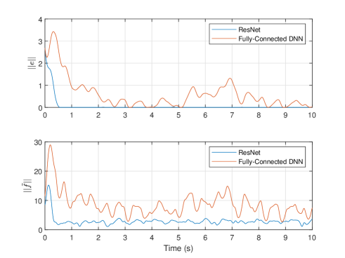
Figure 2: Plots of the tracking error norm $\left\|e\right\|$ and function approximation error norm $\left\|\tilde{f}\right\|$ with ResNet and fully-connected DNN-based adaptive controller.

Table I provides the norm of the root mean square (RMS) tracking error, function approximation error, and control input given by $\left\|e_{\mathrm{rms}}\right\|$, $\left\|\tilde{f}_{\mathrm{rms}}\right\|$, and $\left\|u_{\mathrm{rms}}\right\|$, respectively. In comparison to the fully-connected DNN, the ResNet shows 63.93% and 64.77% decrease in the norms of the tracking and function approximation errors, respectively. As shown in Figure 2, the fully-connected DNN exhibits a comparatively poor tracking and function approximation performance. As mentioned in Remark 2, fully-connected DNNs suffer from the vanishing gradient problem. Thus, the fully-connected DNN weights remain approximately constant as shown in Figure 3. Consequently, the fully-connected DNN-based feedforward term fails to compensate for the uncertainty in the system which yields a relatively poor tracking and function approximation. In contrast to the fully-connected DNN, the presence of shortcut connections in the ResNet eliminates the vanishing gradient problem as mentioned in Remark 2. As a result, the ResNet weights are able to compensate for the system uncertainty as shown in Figure 3 which yields improved tracking and function approximation performance. Additionally, the ResNet requires approximately the same control effort as the fully-connected DNN. Therefore, the ResNet improves the tracking performance without requiring a higher control effort in comparison to the fully-connected DNN.

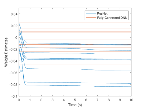
Figure 3: Plot of the weight estimates of the ResNet and fully-connected DNN. There are a total of 2,000 individual weights in each architecture. For better visualization, 10 arbitrarily selected weights are shown. The fully-connected DNN weights adapt slowly due to the problem of vanishing gradients. However, the ResNet weights are able to adapt faster since the ResNet does not have vanishing gradients.

V Conclusion and Future Work

This paper provides the first result on Lyapunov-derived adaptation laws for the weights of each layer of a ResNet-based adaptive controller. A nonsmooth Lyapunov-based analysis is provided to guarantee asymptotic tracking error convergence. Comparative Monte Carlo simulations are provided to demonstrate the performance of the developed ResNet-based adaptive controller. The developed ResNet-based adaptive controller provides approximately 64% improvement in the tracking and function approximation performance, in comparison to an equivalent fully-connected DNN-based adaptive controller. Additionally, the ResNet overcomes the vanishing gradient problem present in the fully-connected DNN.

Future work can explore incorporating a long short-term memory component in the ResNet architecture, based on our recent work [37], to model uncertainties with long-term temporal dependencies. Additionally, composite adaptive methods can be explored that incorporate a prediction error of the uncertainty, in addition to the tracking error, in the adaptation law.

References

- [1] P. Kidger and T. Lyons, “Universal approximation with deep narrow networks,” in Conf. Learn. Theory, pp. 2306–2327, 2020.
- [2] S. L. Brunton and J. N. Kutz, Data-driven science and engineering: Machine learning, dynamical systems, and control. Cambridge University Press, 2019.
- [3] F. Lewis, A. Yesildirek, and K. Liu, “Multilayer neural net robot controller: structure and stability proofs,” IEEE Trans. Neural Netw., vol. 7, no. 2, pp. 388–399, 1996.
- [4] F. L. Lewis, S. Jagannathan, and A. Yesildirak, Neural network control of robot manipulators and nonlinear systems. Philadelphia, PA: CRC Press, 1998.
- [5] S. S. Ge, C. C. Hang, T. H. Lee, and T. Zhang, Stable Adaptive Neural Network Control. Boston, MA: Kluwer Academic Publishers, 2002.
- [6] P. M. Patre, W. MacKunis, K. Kaiser, and W. E. Dixon, “Asymptotic tracking for uncertain dynamic systems via a multilayer neural network feedforward and RISE feedback control structure,” IEEE Trans. Autom. Control, vol. 53, no. 9, pp. 2180–2185, 2008.
- [7] P. Patre, S. Bhasin, Z. D. Wilcox, and W. E. Dixon, “Composite adaptation for neural network-based controllers,” IEEE Trans. Autom. Control, vol. 55, no. 4, pp. 944–950, 2010.
- [8] R. Sun, M. Greene, D. Le, Z. Bell, G. Chowdhary, and W. E. Dixon, “Lyapunov-based real-time and iterative adjustment of deep neural networks,” IEEE Control Syst. Lett., vol. 6, pp. 193–198, 2022.
- [9] G. Joshi and G. Chowdhary, “Deep model reference adaptive control,” in Proc. IEEE Conf. Decis. Control, pp. 4601–4608, 2019.
- [10] G. Joshi, J. Virdi, and G. Chowdhary, “Asynchronous deep model reference adaptive control,” in Conf. Robot Learn., 2020.
- [11] D. Le, M. Greene, W. Makumi, and W. E. Dixon, “Real-time modular deep neural network-based adaptive control of nonlinear systems,” IEEE Control Syst. Lett., vol. 6, pp. 476–481, 2022.
- [12] O. Patil, D. Le, M. Greene, and W. E. Dixon, “Lyapunov-derived control and adaptive update laws for inner and outer layer weights of a deep neural network,” IEEE Control Syst Lett., vol. 6, pp. 1855–1860, 2022.
- [13] I. Goodfellow, Y. Bengio, A. Courville, and Y. Bengio, Deep Learning, vol. 1. MIT press Cambridge, 2016.
- [14] K. He, X. Zhang, S. Ren, and J. Sun, “Deep residual learning for image recognition,” in Proc. IEEE Conf. Comput. Vis. Pattern Recognit., pp. 770–778, 2016.
- [15] M. Hardt and T. Ma, “Identity matters in deep learning,” Int. Conf. Learn. Represent., 2017.
- [16] K. Nar and S. Sastry, “Residual networks: Lyapunov stability and convex decomposition,” arXiv preprint arXiv:1803.08203, 2018.
- [17] Y. Tai, J. Yang, and X. Liu, “Image super-resolution via deep recursive residual network,” in Proc. IEEE Conf. Comput. Vis. Pattern Recognit., pp. 3147–3155, 2017.
- [18] J. Li, F. Fang, K. Mei, and G. Zhang, “Multi-scale residual network for image super-resolution,” in Proc. Eur. Conf. Comput. Vis., pp. 517–532, 2018.
- [19] M. Boroumand, M. Chen, and J. Fridrich, “Deep residual network for steganalysis of digital images,” IEEE Trans. Inf. Forensics Secur., vol. 14, no. 5, pp. 1181–1193, 2018.
- [20] T. Tan, Y. Qian, H. Hu, Y. Zhou, W. Ding, and K. Yu, “Adaptive very deep convolutional residual network for noise robust speech recognition,” IEEE/ACM Trans. Audio, Speech, Language Process., vol. 26, no. 8, pp. 1393–1405, 2018.
- [21] O. S. Patil, D. M. Le, E. Griffis, and W. E. Dixon, “Deep residual neural network (ResNet)-based adaptive control: A Lyapunov-based approach,” in Proc. IEEE Conf. Decis. Control, 2022.
- [22] B. E. Paden and S. S. Sastry, “A calculus for computing Filippov’s differential inclusion with application to the variable structure control of robot manipulators,” IEEE Trans. Circuits Syst., vol. 34, pp. 73–82, Jan. 1987.
- [23] D. S. Bernstein, Matrix Mathematics. Princeton university press, 2009.
- [24] H. Lin and S. Jegelka, “ResNet with one-neuron hidden layers is a universal approximator,” Adv. Neural Inf. Process. Syst., vol. 31, 2018.
- [25] P. Tabuada and B. Gharesifard, “Universal approximation power of deep residual neural networks via nonlinear control theory,” in Int. Conf. Learn. Represent., 2020.
- [26] F. L. Lewis, A. Yegildirek, and K. Liu, “Multilayer neural-net robot controller with guaranteed tracking performance,” IEEE Trans. Neural Netw., vol. 7, pp. 388–399, Mar. 1996.
- [27] A. M. Annaswamy, F. P. Skantze, and A.-P. Loh, “Adaptive control of continuous time systems with convex/concave parametrization,” Automatica, vol. 34, no. 1, pp. 33–49, 1998.
- [28] A. Kojić, A. M. Annaswamy, A.-P. Loh, and R. Lozano, “Adaptive control of a class of nonlinear systems with convex/concave parameterization,” Syst. Control Lett., vol. 37, no. 5, pp. 267–274, 1999.
- [29] W. Lin and C. Qian, “Adaptive control of nonlinearly parameterized systems: the smooth feedback case,” IEEE Trans. Autom. Control, vol. 47, no. 8, pp. 1249–1266, 2002.
- [30] W. Lin and C. Qian, “Adaptive control of nonlinearly parameterized systems: a nonsmooth feedback framework,” IEEE Trans. Autom. Control, vol. 47, pp. 757–774, May 2002.
- [31] Z. Qu, R. A. Hull, and J. Wang, “Globally stabilizing adaptive control design for nonlinearly-parameterized systems,” IEEE Trans. Autom. Control, vol. 51, pp. 1073–1079, June 2006.
- [32] S. B. Roy, S. Bhasin, and I. N. Kar, “Robust gradient-based adaptive control of nonlinearly parametrized plants,” IEEE Control Syst. Lett., vol. 1, no. 2, pp. 352–357, 2017.
- [33] N. Fischer, R. Kamalapurkar, and W. E. Dixon, “LaSalle-Yoshizawa corollaries for nonsmooth systems,” IEEE Trans. Autom. Control, vol. 58, pp. 2333–2338, Sep. 2013.
- [34] F. H. Clarke, Optimization and nonsmooth analysis. SIAM, 1990.
- [35] D. Shevitz and B. Paden, “Lyapunov stability theory of nonsmooth systems,” IEEE Trans. Autom. Control, vol. 39 no. 9, pp. 1910–1914, 1994.
- [36] P. Ioannou and J. Sun, Robust Adaptive Control. Prentice Hall, 1996.
- [37] E. Griffis, O. Patil, Z. Bell, and W. E. Dixon, “Lyapunov-based long short-term memory (Lb-LSTM) neural network-based control,” IEEE Control Syst. Lett., vol. 7, pp. 2976–2981, 2023.