Deep Generative Sampling in the Dual Divergence Space:
A Data-efficient & Interpretative Approach for Generative AI

Abstract

Building on the remarkable achievements in generative sampling of natural images, we propose an innovative challenge, potentially overly ambitious, which involves generating samples of entire multivariate time series that resemble images. This would prove to be a valuable tool for professionals like neurologists, psychiatrists, environmentalists, and economists, among others. However, the statistical challenge lies in the small sample size, sometimes consisting of a few hundred subjects. This issue is especially problematic for deep generative models that follow the conventional approach of generating samples from a standard distribution and then decoding or denoising them to match the true data distribution. In contrast, our method is grounded in information theory and aims to implicitly characterize the distribution of images, particularly the (global and local) dependency structure between pixels. We achieve this by empirically estimating its KL-divergence in the dual form with respect to the respective marginal distribution. This enables us to perform generative sampling directly in the optimized one-dimensional dual divergence space. Specifically, in the dual divergence space, training samples representing the data distribution are embedded in the form of various clusters between two end points. In theory, any sample embedded between those two end points is in-distribution (ID) w.r.t. the data distribution. Our key idea for generating novel samples of images is to interpolate between the clusters via a walk as per gradients of the dual function w.r.t. the data dimensions. In addition to the data efficiency gained from direct sampling, we propose an algorithm that offers a significant reduction in sample complexity for estimating the divergence of the data distribution with respect to the marginal distribution. We provide strong theoretical guarantees along with an extensive empirical evaluation using many real-world datasets from diverse domains, establishing the superiority of our approach w.r.t. state-of-the-art deep learning methods.

1 Introduction

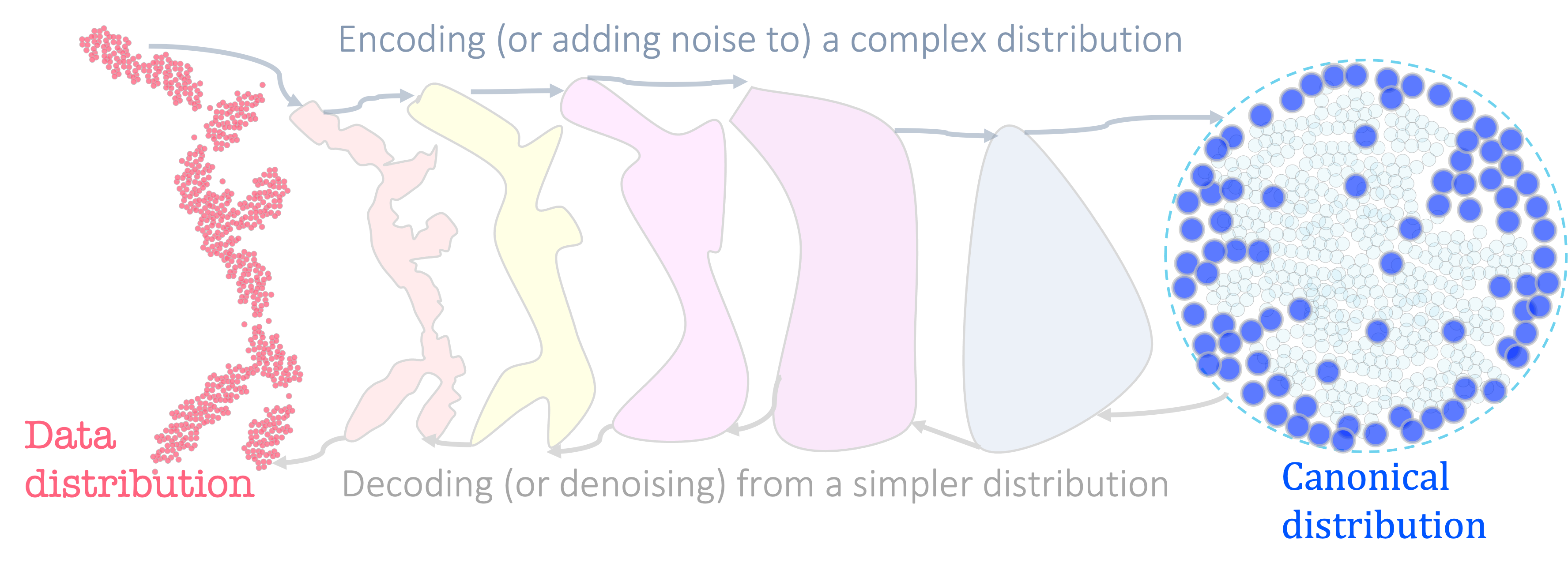
Figure 1: An illustration of the general paradigm followed by most approaches in the literature of deep generative sampling. The data distribution (represented by red dots) gradually evolves into a simpler canonical distribution, such as a Gaussian distribution, either through an encoder, as seen in VAEs and NFs, or by adding noise, as is the case in DDPMs. A canonical distribution facilitates the generation of novel samples which are then mapped back into the data distribution via a decoder as in VAEs, NFs, etc., or via a denoising diffusion process as in DDPMs. The intermediate distributions between the data distribution and the canonical distribution are implied in models such as VAEs while being explicit in NFs or DDPMs. One common limitation of these approaches is that they require a large sample size, which is not available for our problem.

Major advancements have been accomplished in the literature of generating natural images, especially owing to the success of denoising diffusion models [14, 26, 25, 18, 7, 15, 30]. One natural question that arises is whether we can translate this success story to other generative problems that have been of lesser interest to the wider community of computer vision. If so, this would present an opportunity to inherently change the way medical practitioners, such as psychiatrists and neurologists, would operate in the future. Consider, for instance, analyzing electroencephalogram (EEG) signals for the entire duration across all the channels for a patient diagnosed with schizophrenia as if it’s a single image. Generating samples of such images characterizing the missing schizophrenia patients can be highly valuable. Other such use cases include analyzing climate variables like pollution, wind or solar energy, city traffic, or stock markets, etc.

To tackle this unique, unexplored problem of generating entire multivariate time series (MVT) that resemble images, we can utilize state-of-the-art algorithms for generative sampling of images and highly expressive neural architectures, such as Vision Transformers (ViTs) [6]. However, this task also presents some novel challenges. For instance, considering the use case of EEG recordings from patients suffering from schizophrenia, the sample size, or the number of patients for whom recordings can be obtained, is extremely limited, typically consisting of a few hundred patients or even fewer. For an optimal use of such a small number of data points in high dimensions, especially in the context of deep learning, we introduce a fundamentally new approach that is rooted in information theory.

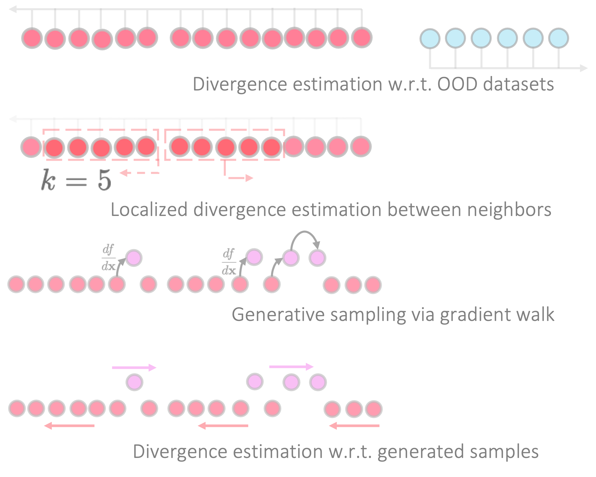
Figure 2: A high-level illustration of our approach for generative sampling. Our key idea is to estimate empirical divergence in its dual form between the observed data points (red dots) and the respective OOD samples (blue dots), so as to implicitly characterize the data distribution of interest in the 1-D dual functional space. The top sketch shows, in the dual space, samples from the two distributions (red vs blue) that are pulled in opposite directions to attain the maximal estimate of the divergence as the optimal measure. The boundary of real samples in the dual space (implicitly) represents the data distribution. For a finer-grained representation of real samples in the dual space, we estimate divergence locally between the nearest neighboring sets. Since the dual space is one-dimensional, it is highly interpretable and straightforward to identify regions (holes) of missing data points. Our algorithm generates (missing) samples in those holes via a gradient walk between the respective clusters. For robustness in generative sampling, we estimate divergence of the observations w.r.t. the generated samples, locally as well as globally.

To understand the motivation behind our novel contributions to generative sampling, we first discuss the general paradigm behind state-of-the-art deep learning approaches for generative sampling, shown in Figure 1. A shared aspect of some of these methods is their reliance on a highly expressive neural decoder as in VAEs [16], Generative Adversarial Networks (GANs) [10, 20, 19, 1, 11, 9], or NFs [21, 4], among others. Another well-established family of score-based methods like DDPMs [14, 26], maps samples generated usually from a canonical base distribution (typically Gaussian) to the data distribution by learning a highly expressive score. In other approaches like f-GANs and Wasserstein GANs, samples are generated such that (empirical) divergence between (the distributions of) generated and observed samples is minimized. Naturally, for training such decoders or denoising processes, one needs a reasonably large sample size, at least many thousands, as typically available for general-purpose natural images. For small datasets, one can imagine that the such machinery is bound to fail due to overfitting.

In consideration of the above, owing to the recent advancements at the intersection of information theory and deep learning, we posit that it is not necessary to sample from a base (canonical) distribution for generating sampling. Instead, it is possible to generate novel samples directly from the one-dimensional dual space of the data distribution which can be obtained by estimating its empirical divergence in the dual form [5] w.r.t. samples from a base canonical distribution (or for that matter, any set of samples deemed as out of distribution). We illustrate this idea in Figure 2. In reference to the figure, besides estimating the dual divergence of the data distribution w.r.t. base (canonical) distribution for representing real samples globally in the dual space, we propose to estimate divergence locally between nearest neighbors within the data distribution (defined as per the global representation of inputs in the dual space itself) so as to learn a fine-grained representation of inputs. We refer the reader to Figure 3 for a more detailed illustration of this particular idea which we refer to as “localized divergence estimation between k-nearest neighbors (kNNs) for multi-scale clustering”. Given a representation of real samples in the dual space, as shown in Figure 2, we propose to generate novel samples simply by a (gradient) walk in the dual space between real samples. To ensure robustness in generating samples that are ID w.r.t. data distribution, we estimate empirical divergence between the two as well. Overall, all the steps mentioned above are performed in an iterative manner for learning the (neural) divergence estimator. Note, although in theory there is a uniquely optimal dual function for estimating divergence between two distributions, we advocate that, in practice, a single expressive neural encoder of images can be universally applied for estimating divergence between different distributions as well as at different scales (local vs global).

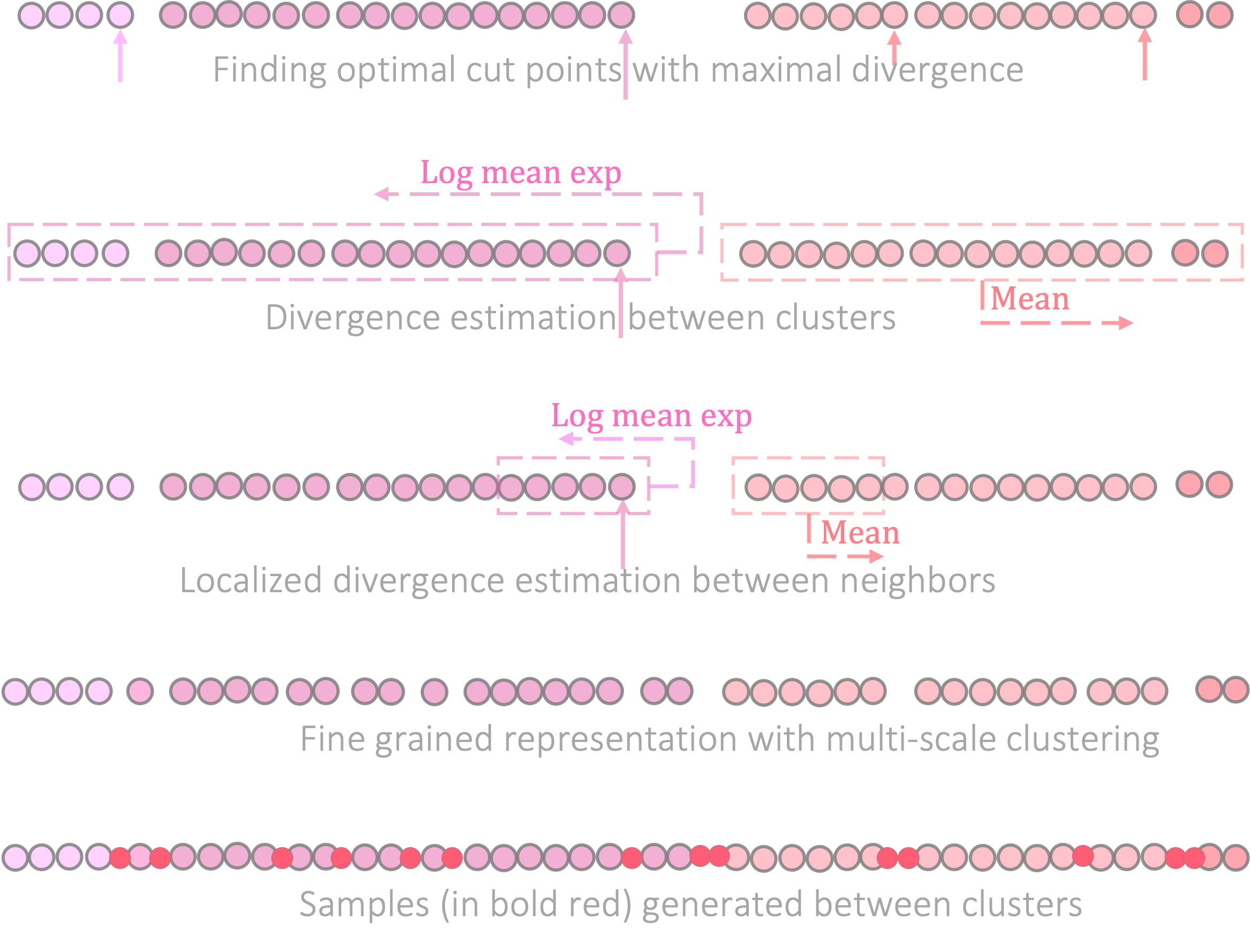
Figure 3: An illustration of our approach for localized divergence estimation at cut points for multi-scale clustering. As established in [8], clusters with maximal (empirical) divergence w.r.t. each other are contiguous in the dual space separated by cut points. As such, the divergence between two clusters at a cut point is estimated by computing softmax and mean statistics using all the samples from the clusters respectively. We instead propose to estimate divergence locally at a cut point by computing the statistics only on the nearest neighbors of the cut point from either side, as shown above. By maximizing localized divergence between neighbors for a small number of cut points while minimizing it on average, we accomplish multi-scale clustering. Having optimized a fine-grained representation of real samples in the dual space, novel samples can be generated in empty space between the clusters (or between distant neighboring data points).

Furthermore, while the proposed approach is generic, we choose to estimate divergence of data distribution specifically w.r.t. the respective marginal distribution (as base distribution) to implicitly model the underlying dependencies between pixels in images, such as those corresponding to neural co-activations in the brain. We argue that it is a particularly suitable choice for our problem of modeling MVT as images, unlike natural images, where it may not suffice to simply have an inductive bias of modeling dependency structure through a choice of neural architecture, such as deep convolutional networks, neither is it practically feasible to learn the dependency structure explicitly, without making any assumptions about it. Moreover, divergence w.r.t. marginals can be estimated with low sample complexity as we propose in this paper; see Figure 4 for details.

Contributions

Our contributions are: (i) We introduce the problem of generative sampling of MVT as an image, and conduct an extensive experimental study, using state-of-the-art deep generative models, for many real-world datasets including EEG recording from patients diagnosed with schizophrenia, spiking neural activity in mouse brains, solar or wind energy, electrical consumption, traffic, pollution, stock returns, etc. (ii) Considering that low sample size is a bottleneck for the success of present methods for the proposed problem, we introduce a novel approach for generative sampling leveraging recent advancements in the literature of divergence estimation via deep learning. Our approach is equipped with efficient algorithms with low sample complexity, and built upon core concepts as introduced above which are simple, intuitive, yet highly effective. (iii) We provide information-theoretic guarantees and demonstrate the empirical superiority of our approach w.r.t. the well-known baselines in the literature of deep generative sampling.

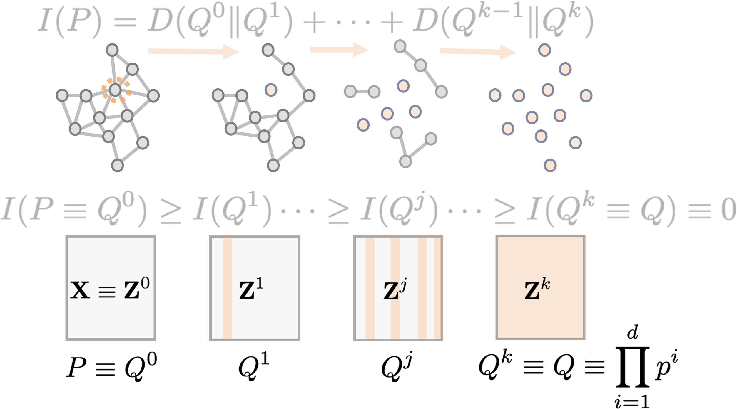
Figure 4: An illustration for sample efficient divergence estimation w.r.t. marginals via dependency diffusion. For an input image, there is an underlying dependency structure between all the dimensions (pixels) which is unknown and never learned explicitly. From the left to right, in each step, we choose a subset of columns in the image and replace the values in there with samples from the respective marginal densities. This, in essence, diffuses the dependencies of the subset of the columns w.r.t. each other (as well as between pixels within each column) and w.r.t. all the other columns as shown in the dependency graphs. In this manner, we obtain samples for all the intermediate densities as well as the marginal distribution without having to learn the density functions or the respective dependency graphs. For each pair of adjacent distributions on the path, $Q^{j-1}$ and $Q^{j}$, we obtain an empirical estimate of $D(Q^{j-1}\|Q^{j})$ in its dual form, and the sum of all the divergence measures along the path gives us an estimate of divergence of the data distribution w.r.t. the marginals, $D(P\|Q)$. The estimation via the path avoids the otherwise exponential sample complexity w.r.t. true measure of $D(P\|Q)$ (in LB by [24]).

2 Deep Generative Sampling in the Dual Space

Let $X\in\mathbb{R}^{d\times d}$ be a random variable corresponding to (unknown) data distribution $P$ of images, and let $Q$ be the respective distribution for the product of the marginals . We are given as input a set of real samples $\mathbf{X}$, representative of the data distribution. Our objective is to generate a set of novel samples, $\mathbf{X}^{g}$, from the data distribution.

First, we introduce core concepts as the basis of our approach for generative sampling, i.e. (sample efficient) divergence estimation of data distribution w.r.t. the marginals in Section 2.1, and local divergence estimation between kNNs in the dual space in Section 2.2. Finally, we present the overall algorithm for generating samples in Section 2.3.

2.1 Dual Divergence Estimation w.r.t. Marginals

We propose to characterize the data distribution by estimating KL-divergence of $Q$ w.r.t. $P$ in its dual form [5] as,

$$D(Q\|P)=\max_{f(.)\in L^{\infty}}\mathbb{E}_{\mathbf{z}\sim Q}\ f(\mathbf{z})-\log\mathbb{E}_{\mathbf{x}\sim P}\ e^{f(\mathbf{x})}.$$ (1)

Here, $f(.)$, is any function from the space of locally $\infty$-integrable functions such that expectations in the expression are finite, referred to as the dual function. Correspondingly, the empirical divergence between samples $\mathbf{X}$ from data distribution $P$ and $\mathbf{Z}$ from marginal distribution $Q$ is defined as,

$$\hat{D}(\mathbf{Z}\|\mathbf{X})=\max_{\hat{f}(.)\in L^{\infty}}\sum_{\mathbf{z}\in\mathbf{Z}}\frac{\hat{f}(\mathbf{z})}{m}-\log\sum_{\mathbf{x}\in\mathbf{X}}\frac{e^{\hat{f}(\mathbf{x})}}{n}$$ (2)

For the empirical estimate of divergence, the dual divergence function $\hat{f}(.)$ can be a deep neural net [2]. For dual representation of images, we can employ any vision architecture such as ViTs [6], CNNs, ResNets [28], etc. For stable learning of the dual function with deep neural nets, standard implementation details such as early stopping, large batch size, low learning rate, gradient clipping, exponential moving averages, are known to be effective in practice [24].

Justifying Marginal as the Base Distribution

The key advantage of taking the product of marginals as the base distribution is its information-theoretic interpretation: the divergence of data distribution w.r.t. the marginals represents the multivariate mutual information among the pixels within an image. This choice of base distribution is particularly suitable for domains such as neuroscience, healthcare, or finance, where marginal distributions are heavily long-tailed and have unique (unknown) dependency structures across input dimensions [3, 22, 17, 27, 12].

Algorithm 1 Estimate divergence locally between kNNs

0:  $\mathbf{X}$, $f(.)$

1:  $\mathbf{f}\leftarrow$ f($\mathbf{X}$);  $\mathbf{f}\leftarrow$ sort($\mathbf{f}$)

2:  for $j=0\to n$ do

3:     $\mathbf{f}_{lnn}\leftarrow\mathbf{f}[j-k:j]$ % kNNs from l.h.s.

4:     $\mathbf{f}_{lnn}\leftarrow\mathbf{f}[j:j+k]$ % kNNs from r.h.s.

5:     $\mathbf{d}_{knn}[j]\leftarrow$ D($\mathbf{f}_{lnn}$, $\mathbf{f}_{rnn}$) % local divergence

6:  end for

7:  Return $\mathbf{d}_{knn}$

2.1.1 Sample Efficient Divergence Estimation via Path

As we illustrate in Figure 4, rather than a direct estimate of divergence between $P$ and $Q$, we propose to estimate it indirectly by establishing a path of diffusing intra- and inter-column dependencies in images towards the base density $Q$.

$$P\equiv Q^{0}\to\cdots\to Q^{j}\to\cdots\to Q^{k}\equiv Q$$ (3)

$$\mathbf{X}\equiv\mathbf{Z}^{0}\to\mathbf{Z}^{1}\to\cdots\to\mathbf{Z}^{j}\to\cdots\to\mathbf{Z}^{k}\equiv\mathbf{Z}$$

$$I(P)\geq\cdots\geq I(Q^{j})\geq\cdots\geq I(Q)\equiv 0$$

Here, $I(.)$ is the multi-variate mutual information function, characterizing dependencies between all the pixels in an image. Our key insight driving the reasoning above is that the divergence of the data distribution w.r.t the product of marginals, $D(P\|Q)$, is equal to the sum of divergence between adjacent distributions along the path of dependency diffusion [29]. The same logic applies to estimating $D(Q\|P)$.

$$D(P\|Q)\equiv D(Q^{0}\|Q^{1})+\cdots+D(Q^{k-1}\|Q^{k})$$ (4)

$$D(Q\|P)\equiv D(Q^{k}\|Q^{k-1})+\cdots+D(Q^{1}\|P)$$

Note that there is no need to explicitly learn the intermediate distributions, $Q^{1},Q^{2},\cdots,Q^{k-1}$, and neither do we need to sample directly from those distributions. We only need to learn the marginal distribution $Q$ which is a tractable problem, from which we take samples $\mathbf{Z}$. Given $\mathbf{X}$ and $\mathbf{Z}$, obtaining samples for the intermediate distributions is straightforward. Thus, we estimate $\hat{D}(\mathbf{Z}\|\mathbf{X})$ indirectly via the path as,

$$\hat{D}(\mathbf{Z}\|\mathbf{X})=\hat{D}(\mathbf{Z}\|\mathbf{Z}^{k-1})+\cdots+\hat{D}(\mathbf{Z}^{1}\|\mathbf{X}).$$ (5)

Accordingly, the respective (normalized) dual function, $\hat{f}_{\eta}(.)$, is also estimated indirectly as,

$$\hat{f}_{\eta}(\mathbf{x}) =\sum_{j=0}^{k-1}f^{j}_{\eta}(\mathbf{x})$$ (6)

$$\hat{f}^{j}_{\eta}(\mathbf{x}) =\hat{f}^{j}(\mathbf{x})-\eta^{f}_{j}$$

$$\eta^{f}_{j} =\log\sum_{\mathbf{z}\in\mathbf{Z}^{j}}e^{f^{j}(\mathbf{z})}-\log(|\mathbf{Z}^{j}|),$$

with dual function $\hat{f}^{j}(.)$ corresponding from estimating $\hat{D}(\mathbf{Z}^{j+1}\|\mathbf{Z}^{j})$. In the following, we establish that sample complexity for estimating the dual function via the path can be exponentially smaller than from the direct estimate.

Sample complexity of the path-based estimator

First, for the sake of completeness, we establish that the proposed divergence estimator via a path of dependency diffusion is consistent. See the supplement for more details. Despite the appeal of divergence estimation in its dual form, the reliability of these estimators has been a topic of debate in the field. One of the most important theoretical results in this regard is due to [24], stating that the variance of the divergence estimate is lower bounded by the exponential of the true divergence. In the following, we argue that it may be possible to avoid the exponential dependence if we estimate it indirectly through the path of dependency diffusion as introduced in Section 2.1.1, in contrast to the direct estimate through a single step.

Algorithm 2 Samples via gradient walk in the dual space

0:  $\mathbf{X}$, $f(.)$

1:  $\mathbf{f}\leftarrow$ f($\mathbf{X}$);  $\mathbf{f}\leftarrow$ sort($\mathbf{f}$)

2:  $\mathbf{d}_{knn}\leftarrow$ estimateLocalDivergence($\mathbf{X}$) % localized divergence estimation between kNNs in the dual space

3:  $\mathbf{c}\leftarrow$ argpartition($\mathbf{d}_{x}$, c) % find indices of cut points with maximal local divergence between the neighbors

4:  for $j=0\to c$ do

5:     $\mathbf{X}^{g}_{j}\leftarrow$ gradWalkDualSpace($f_{c_{j}}$, $f_{c_{j}+1}$) % generate samples between $f_{c_{j}}$ and $f_{c_{j}+1}$ per $\frac{df}{d\mathbf{x}}$

6:  end for

7:  Return $\mathbf{X}_{s}$

Theorem 1.

Variance for the direct estimation of ${D}(P\|Q)$ in its dual form using $n$ samples is,

$$\lim_{n\to\infty}n\ \mathrm{Var}_{P,Q}\hat{D}_{n} \geq-1+e^{D(P\|Q)}$$

$$=-1+\prod_{j=0}^{d-2}e^{D(Q^{j}\|Q^{j+1})},$$ (7)

whereas variance for its estimation via the dependency diffusion path, assuming the divergence estimates for each step to be independent, is:

$$\lim_{n\to\infty}n\mathrm{Var}_{P,Q}\hat{D}_{n}^{ddp}\geq 1-d+\sum_{j=0}^{d-2}e^{D(Q^{j}\|Q^{j+1})}$$ (8)

Here, in Eq. 8, the lower bound for the variance is no longer (exponentially) dependent upon the true measure of $D(P\|Q)\equiv I(P)$, rather dominated by the true measure of maximal divergence between two adjacent distributions on the path. Although it is not guaranteed that one inequality will strictly dominate the other in the worst-case scenario, one can assume that the overall dependency between all pixels in an image is usually greater than the dependency between two columns or rows within an image.

In reference to Figure 2, from estimating divergence of data distribution (red dots) w.r.t. the marginal (blue dots), we obtain global characterization (representation) of data distribution in the dual divergence space. Next, we introduce the idea of localized divergence estimation between nearest neighbors in the dual space, so as to obtain a fine-grained characterization of the data distribution in the dual divergence space.

2.2 Localized Divergence Estimation for Clustering

Besides estimating divergence of the data distribution w.r.t. the respective marginal distribution, we propose to obtain a fine-grained characterization of the data distribution by learning clusters within the input dataset. In particular, we learn clusters such that divergence is maximized between the clusters as originally proposed by [8]. This information-theoretic approach simplifies the problem of clustering to one of finding optimal cut points, the ones with maximal divergence, in the dual divergence space. See Figure 3 and the pseudo-code in Algorithm 1.

Algorithm 3 Overall algorithm for generative sampling

0:  $\mathbf{X}$

1:  $f(.)\leftarrow$ initDualDivFunc($\mathbf{X}$) % (neural) model of images as a dual function to estimate divergence

2:  $\mathbf{Z}\leftarrow$ samplesFromMarginals($\mathbf{X}$)

3:  for $i=0\to t$ do % estimate divergence of inputs w.r.t. the marginals 4:     $\mathbf{f}_{x}\leftarrow$ f($\mathbf{X}$),  $\mathbf{f}_{z}\leftarrow$ f($\mathbf{Z}$) 5:     $d_{xz}\leftarrow$ D($\mathbf{f}_{x}$, $\mathbf{f}_{z}$) % divergence between $\mathbf{X}$ and $\mathbf{Z}$ 6:     $f(.)\leftarrow$ backPropagate($f(.)$, $-d_{xz}$) % local divergence estimation between neighbors 7:     $\mathbf{d}_{knn}\leftarrow$ estimateLocalDivergence($\mathbf{X}$) 8:     $l_{c}\leftarrow\sum_{j}\mathbf{d}_{knn}[j]-\log\sum_{j}e^{\mathbf{d}_{knn}[j]}$ % clustering loss from the local divergence estimation 9:     $f(.)\leftarrow$ backPropagate($f(.)$, $l_{c}$)

10:     if $i\geq t_{w}$ then % sample via gradient walk in the dual space 11:        $\mathbf{X}^{g}\leftarrow$ sampleViaGradientWalk($\mathbf{X}$, $f(.)$) 12:        $\mathbf{f}_{g}\leftarrow$ f($\mathbf{X}^{g}$) 13:        $\hat{D}_{xg}\leftarrow$ D($\mathbf{f}_{x}$, $\mathbf{f}_{g}$) % divergence w.r.t. samples 14:        $f(.)\leftarrow$ backPropagate($f(.)$, $-\hat{D}_{xg}$)

15:     end if

16:  end for

17:  $\mathbf{X}^{g}\leftarrow$ sampleViaGradientWalk($\mathbf{X}$, $f(.)$)

18:  Return $\mathbf{X}^{g}$ % return generated samples

As we show in Figure 3, we propose to have a more localized estimate of divergence at cut points, i.e. divergence between k-nearest neighbors on either side of the cut point. This approach is particularly well-suited to our problem context, where clustering is a secondary objective aimed at learning refined representations of data points in the dual divergence space. Moreover, for the same reason, the number of clusters $c$ in our problem setting is not a fixed (small) number. Rather, owing to the localized divergence estimation at cut points, we learn as many clusters as possible by maximizing softmax ($logsumexp$) of divergence on all the cut points while minimizing the mean statistic for the same. The former can be thought of as inter-cluster divergence and the latter as intra-cluster divergence. Effectively, as illustrated in the figure, we obtain clustering at different scales. As shown in the figure, we can generate novel samples in empty dual space between the clusters.

2.3 Overall Algorithm for Generative Sampling

In the previous sections, we have introduced two fundamental concepts for characterizing the data distribution in the dual space. The first concept involves estimating the divergence between the data distribution and its respective marginal distributions, in order to represent the dependencies between input dimensions (pixels). The second involves estimating the divergence locally between nearest neighbors, in order to achieve a fine-grained representation of data points within the data distribution. Overall, in our proposed approach, we employ a (single) neural model that learns to estimate the divergences in an iterative manner.

In Algorithm 3, in each iteration, the neural model updates its weights to increase the empirical estimate (in the dual form) of divergence of data distribution w.r.t. the marginals, as well as to decrease the clustering loss estimated from the localized divergence estimation. Further, within the same iteration, novel samples are generated in the presently optimized dual space via gradient walk in the empty spaces between the clusters (see Algorithm 2 for more details). Note that the neural model learns to estimate the divergence of data distribution w.r.t. generated samples as well. The intuition behind the latter step is that some of the generated samples may be out of distribution w.r.t. the data distribution. This could arrive due to noisy gradients of the dual function w.r.t. inputs. Estimating divergence w.r.t. samples filters out the OOD samples as well as robustifies the estimation of dual function gradient in the empty space between clusters.

We establish that the divergence of generated samples w.r.t. data distribution can be bounded as below.

Theorem 2.

An empirical estimate of the KL divergence between real samples $X$ and generated samples $X_{g}$ using Eq. 2, can be bounded as $\hat{D}(X_{g}\|X)=O(d^{knn}_{max})$ where $d^{knn}_{max}$ is the maximal distance of a point from $X_{g}$ to its nearest point in $X$ in the one-dimensional dual functional space of both the sets.

Since we generate novel samples in empty space between clusters in the dual space, as per the above theorem, it reduces the empirical divergence of generated samples w.r.t. real samples as a consequence of the reduction in the maximal kNNs distance ($d^{knn}_{max}$) between the two sets.

3 Experiments

We conduct experiments for the problem of generating novel samples of entire multivariate timeseries as images, using several datasets from a diverse set of domains as described below.

(a) EEG

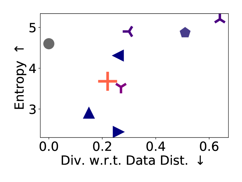
(b) Neuropixels

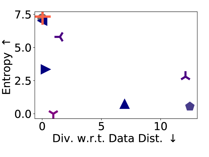
(c) Stock Returns

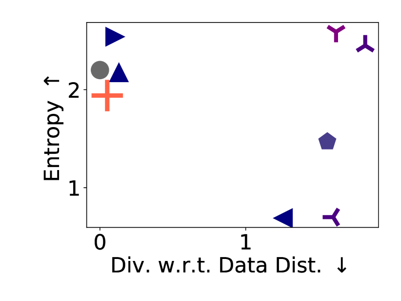
(d) City Traffic

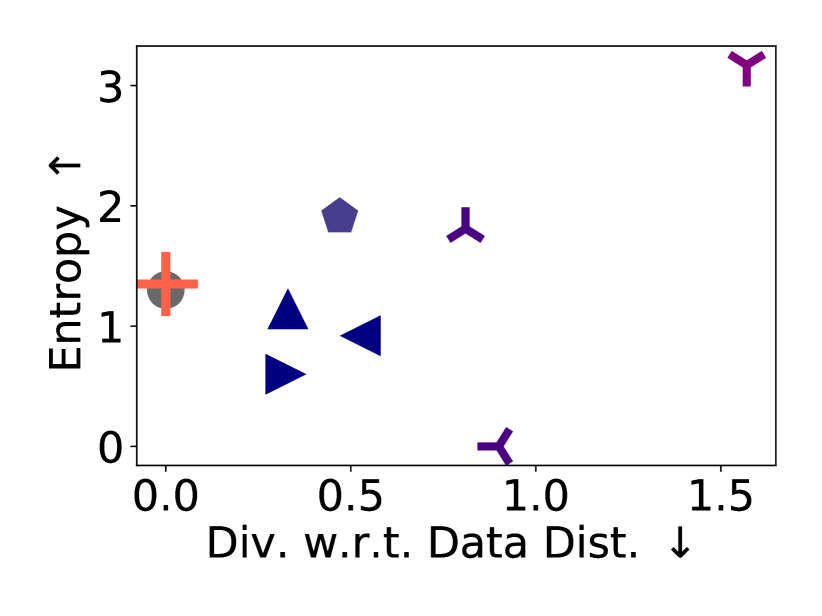
(e) Air Pollution

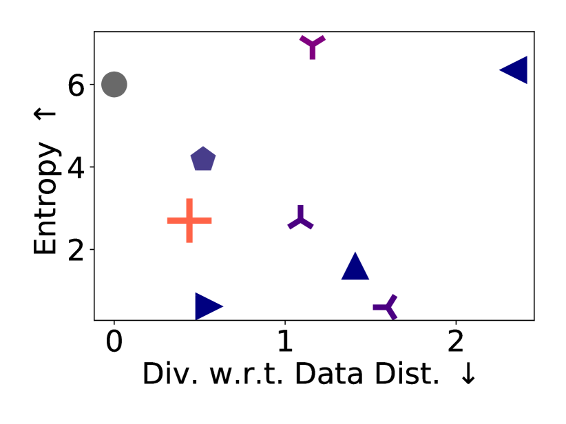
(f) Wind Farms

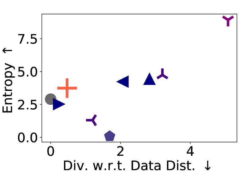
(g) Solar Energy

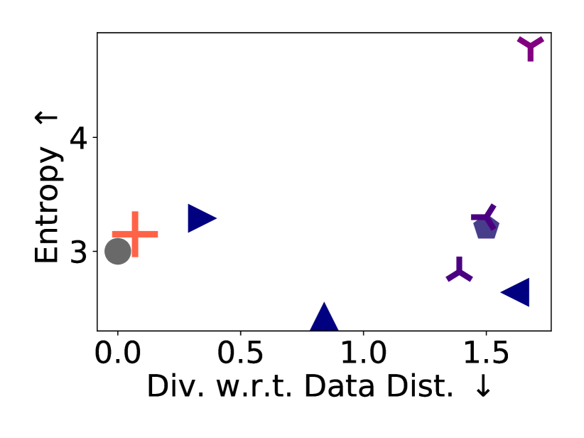
(h) Electrical Consumption

Figure 5: All the methods are compared in terms of KL-Divergence of generated samples w.r.t. data distribution which is desired to be minimized while maximizing entropy of the generated samples.

Datasets

(i) EEG: We are interested in analyzing the electrical activity in the brains of 81 patients diagnosed with schizophrenia, utilizing data from 74 channels per patient. After preprocessing, we obtain 81 real samples of images each of dimension 72x72. (ii) Neuropixels: We model spiking neural activity over a 2-second period, capturing data from diverse regions within mouse brains using 443 high-density extracellular electrophysiology probes [23]. Derived from numerous recording sessions, we acquired 195 preprocessed images, each of dimension 96x96. The preprocessing included the exclusion of probes exhibiting minimal activity. (iii) Stock Returns: We analyze returns for the 50 most liquid securities from the Russell 3000 index with each month from the past corresponding to a single image resulting in a dataset of 160 images, each of size 48x48. (iv) City Traffic: In the city of San Francisco, it is valuable to study hourly traffic across multiple sites in the city. Viewing weekly traffic as a single image, we obtain a dataset of 104 images, each of dimension 168x168. (v) Air Pollution: Air quality indices are analyzed on an hourly basis for major cities across the world (aka KDD Cup 2018). Similar to the traffic dataset, we view weekly pollution data as a single image and obtain a dataset of 56 images, each of dimension 168x168. (vi) Wind Farms: Wind power production is recorded across wind farms in Australia. Analyzing it every 12 hours as an image, we obtain a dataset of 732 images, each of size 144x144. (vii) Solar Energy: Solar power data is measured every 10 minutes at many eastern U.S. locations. Considering the high inter- and intra-day dynamics of solar energy, we preprocess the data to analyze solar energy variation in a day as a single image. This results in a dataset with 386 images, each of size 136x136. (viii) Electrical Consumption: Electricity consumption was recorded every hour at 370 sites from year 2012 to 2014. We preprocess the data and obtain the weekly electricity consumption as a single image. This results in a dataset of 156 images, each of size 168x168. (Additional information about these datasets is available in the supplement.)

Baselines

To illustrate the efficacy of the proposed approach, we evaluate its performance against various established methods for deep generative sampling of images. Specifically, we employ (i) VAE [16], (ii) GAN [10], (iii) WGAN [1], (iv) f-GAN [20], (v) NF [21], (vi) DDPM [14], and (vii) DDPM via stochastic differential equation (SDEs) (DDPM-SDE) [26].

Evaluation Settings

For each method of generative sampling, we explore different choices of architectures for modeling including Convolutional Neural Networks (CNNs), ViTs, or even Feedforward Neural Networks (FNNs) in some cases. In addition to standard encoding of patches within images, we also found it useful to encode all the rows and columns within an image (aka horizontal or vertical patches). While leveraging the official implementations of the baseline methods, considering the (very) small size of training sets, we utilized different strategies to avoid overfitting including dropout, $l_{2}$ regularization, and lighter-weight architecture in terms of the number of layers, among others (see more details in the supplement). For each dataset, we generate 1000 samples from every method and evaluate the samples in terms of diversity, novelty, and being ID w.r.t. data distribution as discussed next.

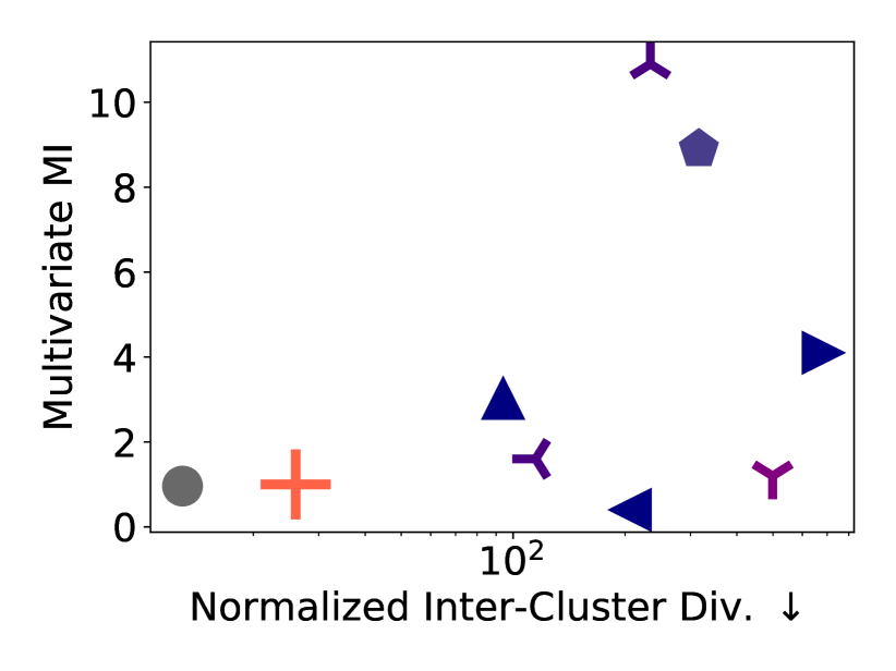
(a) EEG

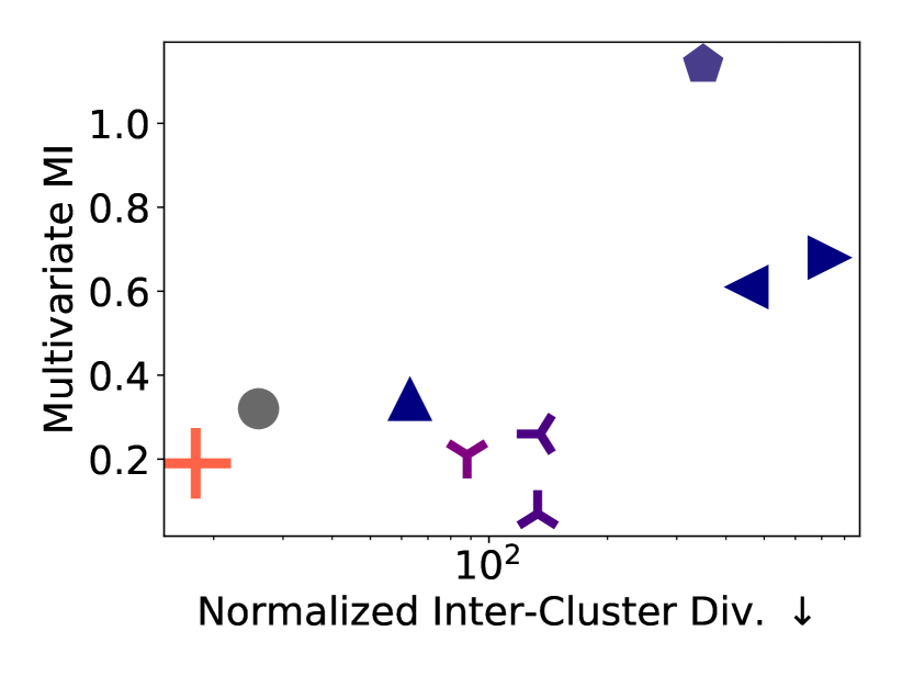
(b) Neuropixels

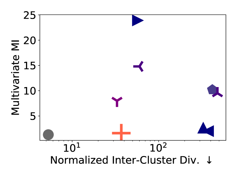
(c) Stock Returns

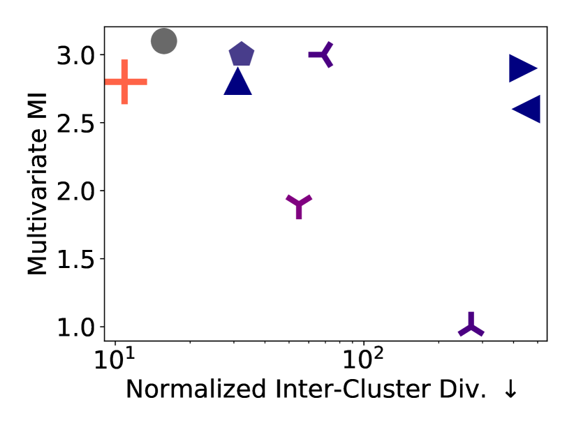
(d) Traffic

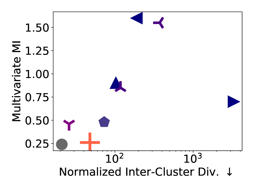
(e) Pollution

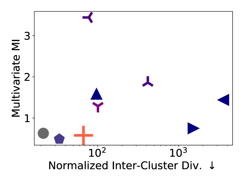
(f) Wind Farms

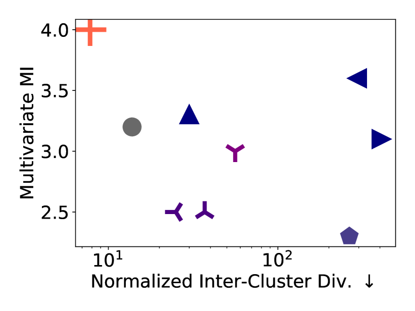
(g) Solar Energy

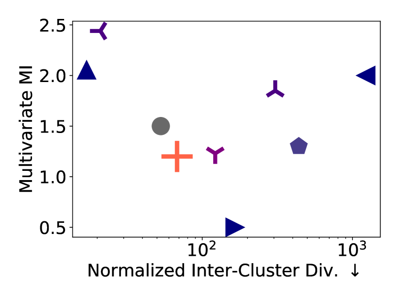
(h) Electrical Consumption

Figure 6: All the methods are evaluated based on two metrics. On the X-axis, we plot (normalized) maximal (empirical) divergence between clusters within the union set of input and generated samples. This measure is desired to be minimized ($\downarrow$), as an indirect proxy for the diversity of generated samples vs real samples. On the Y-axis, we plot estimated MMI between pixels of images (dimensions of samples). MMI for generated samples should close in value to the MMI for real samples.

3.1 Evaluation Results

Assessing methods for generating image samples is as intricate as the problem itself, given their inherent interdependence. Unlike the case of natural images where a pre-trained deep neural network (DNN) (such as InceptionV3) is available for obtaining feature representations of generated images, modeled as multivariate Gaussian so as to measure Fréchet Inception Distance (FID) between the two distributions of images (real and generated) [13], there is no such standardized model to obtain representation of images for our problem. Moreover, assuming the representations of images from a DNN like InceptionV3 to be Gaussian distributed may suffice in practice for natural images, but not necessarily for other possible kinds of images like the ones considered in this paper. Nevertheless, we present a comparison of all the methods as per an FID score in Table 1, establishing superiority of our approach upon all the baselines. 

Dataset	VAE	W-GAN	GAN	f-GAN	NF	DDPM-SDE	DDPM	Ours
EEG	1.03$\pm$0.0	0.61$\pm$0.03	0.71$\pm$0.09	1.34$\pm$0.17	0.15$\pm$0.02	1.2$\pm$0.02	0.34$\pm$0.04	0.12$\pm$0.06
NeuroPixels	6.44$\pm$0.00	0.78$\pm$0.02	1.85$\pm$0.05	1.0$\pm$0.04	0.97$\pm$0.03	3.71$\pm$0.10	1.19$\pm$0.10	0.26$\pm$0.05
Stock Returns	5.21$\pm$0.02	4.43$\pm$0.09	1.2$\pm$0.08	2.16$\pm$0.25	10.43$\pm$0.30	5.78$\pm$0.10	3.8$\pm$0.15	0.32$\pm$0.21
Traffic	4.46$\pm$0.11	3.49$\pm$0.50	26.42$\pm$0.98	1.65$\pm$0.26	9.85$\pm$0.58	36.93$\pm$0.10	20.16$\pm$0.18	0.51$\pm$0.12
Pollution	0.22$\pm$0.04	0.11$\pm$0.0	0.25$\pm$0.01	0.34$\pm$0.02	0.73$\pm$0.02	0.78$\pm$0.01	0.15$\pm$0.01	0.03$\pm$0.00
Wind Farms	1.31$\pm$0.06	6.85$\pm$0.12	19.29$\pm$0.0	10.35$\pm$0.34	4.11$\pm$0.07	12.2$\pm$0.04	10.56$\pm$0.33	0.48$\pm$0.09
Solar Energy	25.88$\pm$0.0	0.85$\pm$0.07	4.58$\pm$0.60	9.4$\pm$0.21	42.91$\pm$0.59	26.74$\pm$0.03	9.55$\pm$0.28	0.70$\pm$0.18
Electrical Consumption	4.94$\pm$0.02	1.1$\pm$0.06	9.56$\pm$0.01	23.15$\pm$0.27	8.2$\pm$0.40	18.06$\pm$0.05	4.8$\pm$0.25	0.36$\pm$0.06

Table 1: FID scores ($\downarrow$) for generated samples. For a set of generated samples from a method which is larger in size (1000) than the original sample size, we randomly select samples from the set as many as the real samples to obtain FID score. Having performed 100 trials, we obtain mean and standard deviation of FID scores for a given method. Our method obtains the lowest FID scores w.r.t. all the other methods.

Because of the aforementioned limitations of FID metric, for the primary analysis, we introduce four advanced (information theoretic) evaluation metrics, estimated without any distribution assumptions or a pre-trained network, as discussed below. The first metric measures the (empirical) divergence of generated samples w.r.t. data distribution (i.e. training set of real samples). It aims to verify whether the generated samples accurately represent the underlying data distribution. While akin to FID, this metric is computed directly on raw images without making any distributional assumptions. Nevertheless, relying solely on this metric can be misleading in cases of overfitting. To address this, we propose to measure the (empirical) entropy of generated samples, estimated via its KL-divergence w.r.t. uniform distribution, as a proxy for the diversity of samples. Before introducing the other two metrics, in reference to Figure 5, we first discuss our evaluation results as per these two metrics. For datasets, EEG, stock returns, and electricity consumption, our approach dominates, exhibiting low divergence and high entropy. In the context of the traffic dataset, our method proves to be highly competitive, with W-GAN and f-GAN generating samples of marginally higher entropy (diversity). However, for the wind farms dataset, GAN outperforms our method, and NF is also highly competitive, albeit with a trade-off of higher divergence of generated samples w.r.t. data distribution. In the case of the solar energy dataset, our approach and W-GAN demonstrate equal competitiveness. DDPM stands out as competitive only for the EEG, neuropixels, and stock returns datasets.

To measure the novelty of generated samples w.r.t. real samples, we introduce a metric in relation to Theorem 2, i.e. (normalized) softmax of divergence between clusters within the joint set of real samples and generated samples. The metric value is inversely proportional to the novelty of the generated samples w.r.t. real samples. In addition, we are also interested in analyzing if generated (image) samples characterize dependencies between pixels as in the original real samples. While it is not possible to estimate dependencies explicitly for comparison between the two sets, we quantify MMI between pixels for real samples vs generated samples. We expect generated samples to have the same MMI value as the real samples. See the comparison between methods as per these two metrics in Figure 6. For datasets, EEG, neuropixels, stock returns, and traffic, our method generates samples with higher novelty w.r.t. other methods while maintaining MMI similar to real samples. For the pollution dataset, when comparing NF to our method, there is a trade-off. A similar trade-off appears for electrical consumption and solar energy datasets. For the wind farms dataset, our method is the most competitive after GAN.

Evaluation using supplementary metrics

Besides the primary evaluation as discussed above, in Table 2, we present our analysis using four supplementary evaluation metrics. The first metric is Inception score (aka IS in the literature) as a proxy for the diversity of samples. This is estimated using the original Inception-v3 model itself. Using Inception-v3, we also estimate the most popular metric FID. Note that the FID scores reported above in Table 1 are different from the ones presented here in Table 2 as the former ones are estimated using a neural MI estimator. Moreover, similar in spirit to the KL-divergence metric (Figure 5), we evaluate generated samples in terms of the Wasserstein distance aka WD (as in W-GAN) w.r.t. the real samples. Lastly, we estimate negative log likelihood (NLL) of generated samples using a DDPM. Overall, across all the metrics and 8 datasets, our method consistently outperforms the competitive approaches.

Data	Metric	VAE	wGAN	GAN	fGAN	NF	DDPMsde	DDPM	Ours
EEG	IS$\uparrow$	1.0	1.3	2.6	5.4	2.0	1.5	1.9	3.1
	FID$\downarrow$	0.52	0.28	0.13	1.04	0.15	0.40	0.25	0.11
	WD$\downarrow$	8.45	3.29	0.27	2.65	0.13	14.41	0.50	0.26
	NLL$\downarrow$	0.18	0.05	0.05	0.46	0.06	0.21	0.03	0.01
NP	IS$\uparrow$	1.2	2.1	3.2	2.5	2.5	2.3	3.8	2.8
	FID$\downarrow$	0.56	0.40	0.69	0.46	0.29	0.49	0.14	0.10
	WD$\downarrow$	0.87	0.28	0.42	0.18	0.12	0.15	0.16	0.05
	NLL$\downarrow$	0.24	0.05	0.15	0.12	0.13	0.24	0.06	0.07
SR	IS$\uparrow$	1.0	1.4	1.1	1.2	1.5	1.5	1.4	3.4
	FID$\downarrow$	1.22	0.24	0.19	1.34	0.37	1.11	0.14	0.05
	WD$\downarrow$	12.62	20.17	0.43	7.23	48.94	30.86	8.53	3.32
	NLL$\downarrow$	0.15	0.08	0.01	0.41	0.09	0.19	0.01	0.03
CT	IS$\uparrow$	2.2	1.6	2.2	2.2	3.4	1.8	2.3	4.7
	FID$\downarrow$	0.53	0.31	0.88	0.36	0.23	1.14	0.33	0.08
	WD$\downarrow$	1.57	0.10	1.29	0.13	0.74	1.43	1.67	0.15
	NLL$\downarrow$	0.12	0.08	0.09	0.06	0.14	0.34	0.06	0.01
AP	IS$\uparrow$	10.4	1.7	1.7	4.5	4.5	1.8	10.4	10.6
	FID$\downarrow$	0.74	1.07	1.12	0.65	0.77	1.04	0.53	0.15
	WD$\downarrow$	0.58	0.43	1.11	0.75	0.34	0.86	1.33	0.02
	NLL$\downarrow$	0.05	0.06	0.12	0.19	0.21	0.29	0.03	0.01
WF	IS$\uparrow$	4.9	3.0	1.0	2.5	6.4	2.3	5.9	5.9
	FID$\downarrow$	0.57	0.78	1.32	1.55	0.63	1.13	0.48	0.17
	WD$\downarrow$	0.28	0.66	1.15	1.51	1.26	1.21	1.53	0.23
	NLL$\downarrow$	0.04	0.05	0.29	0.33	0.07	0.30	0.02	0.01
SE	IS$\uparrow$	1.0	4.3	2.9	3.5	3.4	1.7	10.6	5.8
	FID$\downarrow$	1.77	0.21	0.16	1.4	0.75	1.34	0.32	0.25
	WD$\downarrow$	1.87	0.37	1.96	2.88	4.60	3.23	1.39	1.71
	NLL$\downarrow$	0.01	0.02	0.03	0.42	0.18	0.32	0.02	0.01
EC	IS$\uparrow$	1.2	1.6	1.0	2.0	3.1	1.8	3.8	2.0
	FID$\downarrow$	1.45	0.88	1.52	1.29	1.11	1.63	1.02	0.05
	WD$\downarrow$	0.54	0.25	1.65	1.82	0.61	1.72	1.94	0.10
	NLL$\downarrow$	0.25	0.07	0.19	0.42	0.14	0.29	0.04	0.01

Table 2: Analysis using supplementary evaluation metrics. Due to space constraint, dataset names are abbreviated. The best numbers (within rows) are shown in bold and the second best are in italic.

Visualization of generated samples

In Figure 7, 8, and 9, we show visualization of randomly selected images, both from the original dataset as well as the ones generated by our method. Note, while the images are single channel, we present these as colored ones here simply for more appealing visualization as a practitioner from these data domains would do.

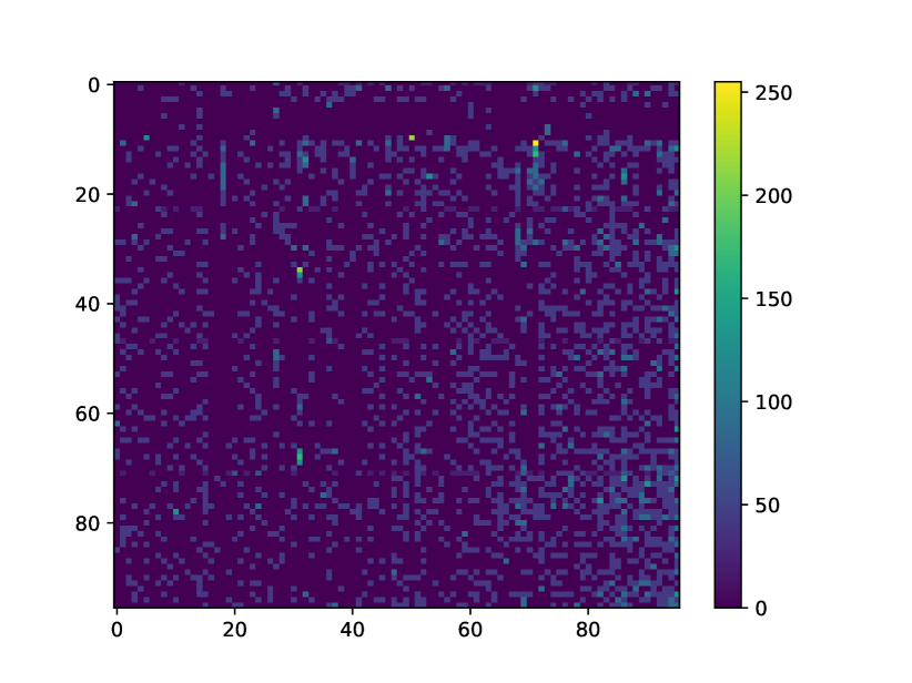
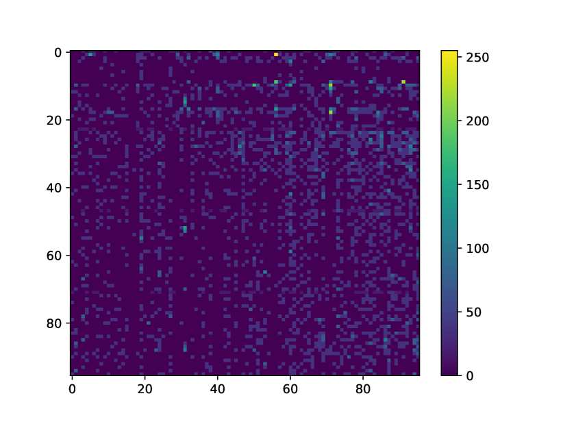
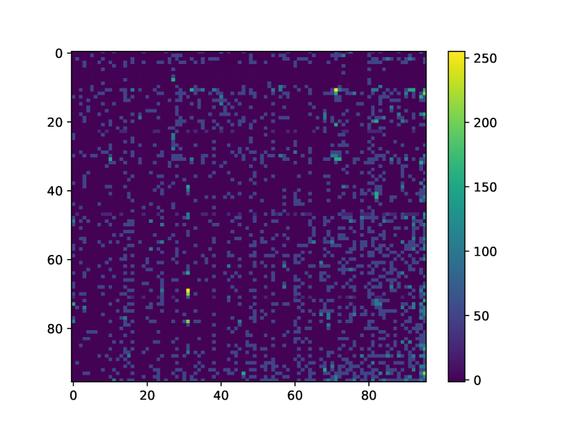
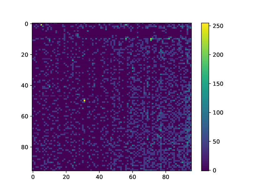
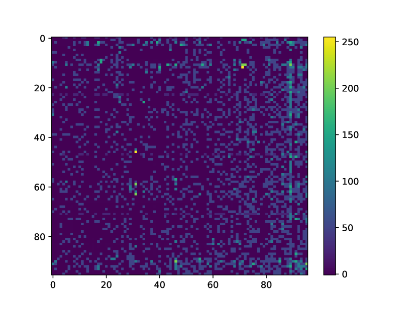
Figure 7: Randomly selected images from Neuropixels datasets. The images in the first row are original images whereas the ones in the second row are generated by our approach.

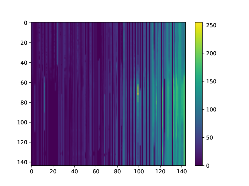
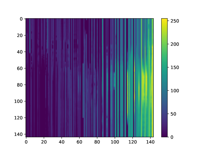
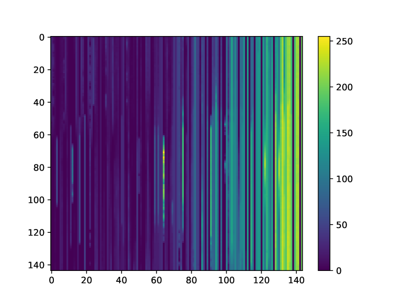
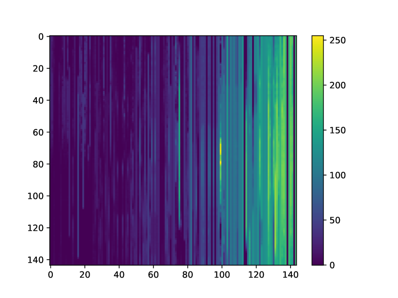
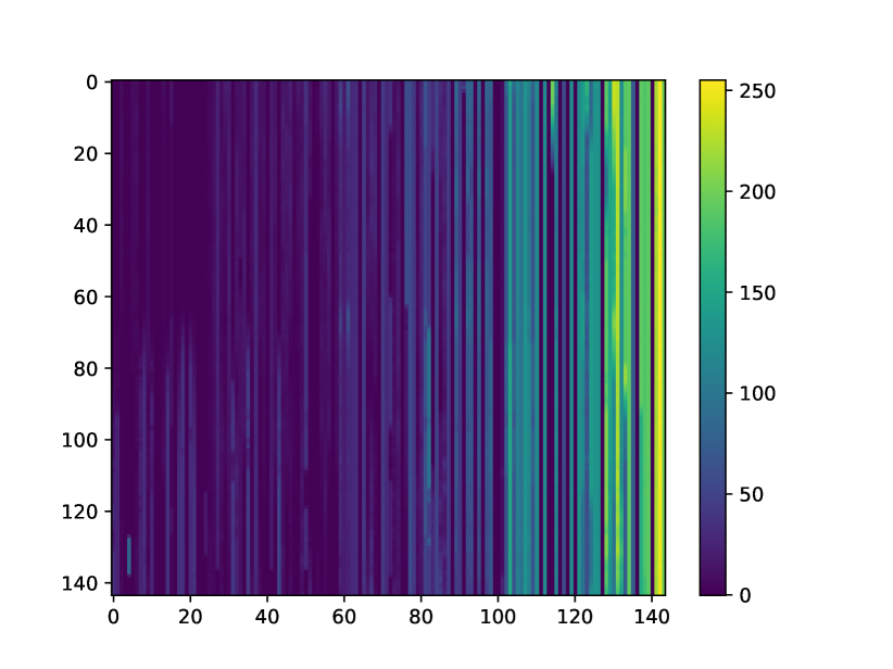
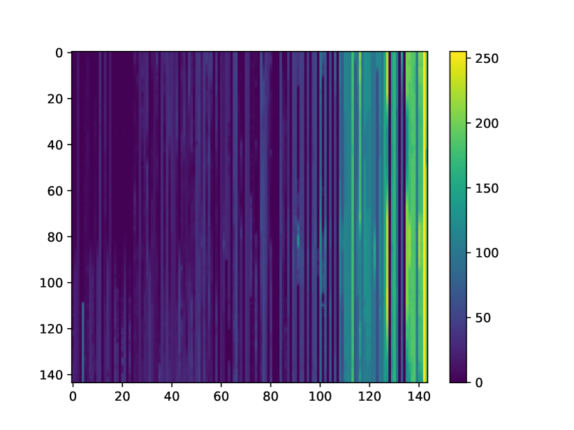
Figure 8: Randomly selected images from Wind Farms dataset. The images in the first row are original images whereas the ones in the second row are generated by our approach.

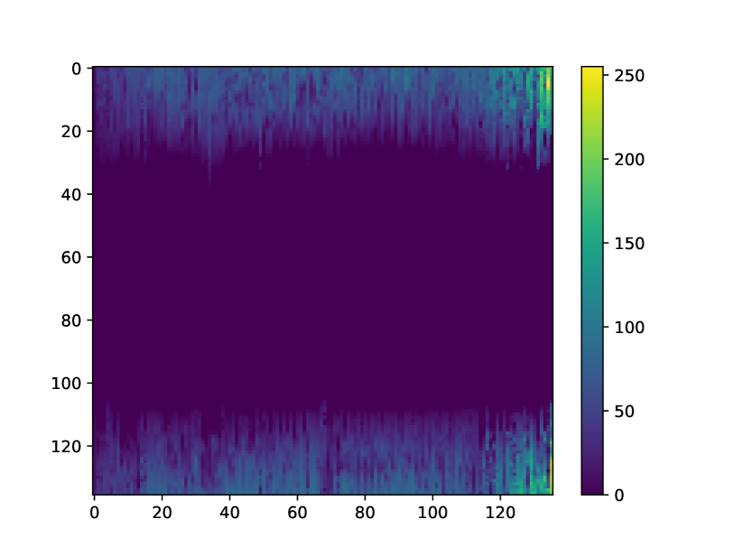
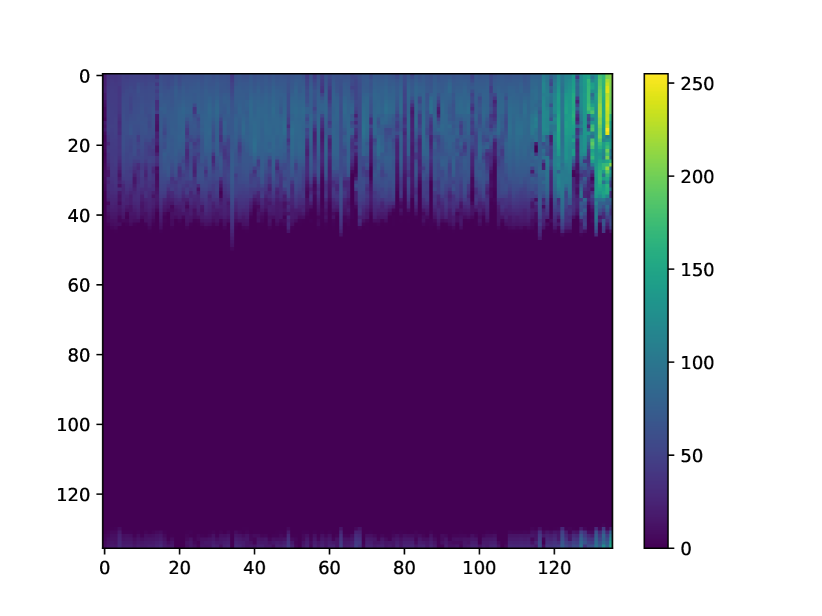
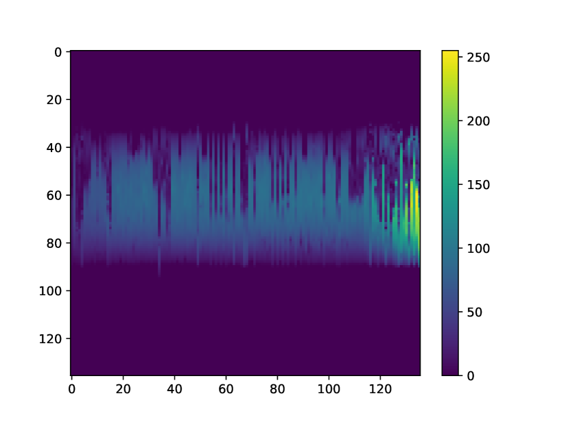
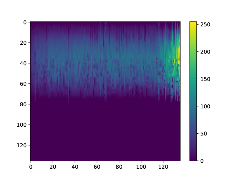
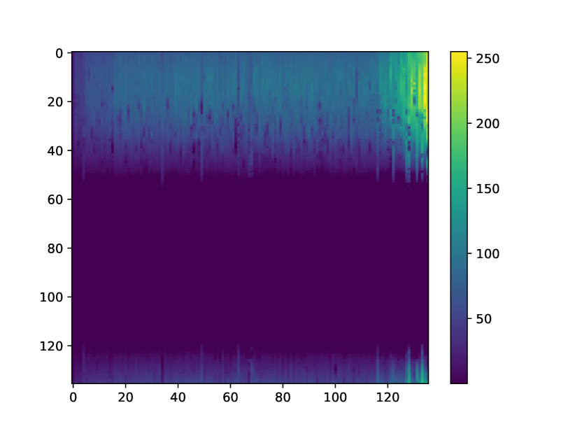
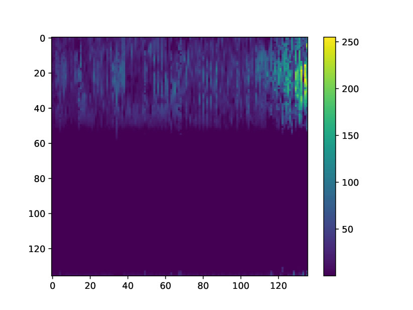
Figure 9: Randomly selected images from Solar Power dataset. The images in the first row are original images whereas the ones in the second row are generated by our approach.

4 Conclusion

We introduced the problem of generating multivariate time-series data in the form of images, with potential applications across diverse domains, including healthcare. Given the inherently small sample sizes in such problems, in contrast to datasets of natural images, state-of-the-art deep learning methods for generative sampling are prone to overfitting. This is due to the fact that in all the methods samples are generated from a canonical distribution and then mapped to data distribution through a highly expressive decoder or denoising diffusion process. To address the issue of sample efficiency, we proposed a deep information theoretic approach for generating samples directly in the dual space of data distribution which is obtained by estimating its divergence in the dual form w.r.t. the respective marginal distribution. Within this framework, we introduced various ideas to ensure robust sampling. Alongside theoretical guarantees, we conducted a comprehensive experimental analysis using several real-world datasets demonstrating the competitiveness of our method in comparison to various established deep generative models.

References

- Arjovsky et al. [2017] Martin Arjovsky, Soumith Chintala, and Léon Bottou. Wasserstein generative adversarial networks. In International conference on machine learning, pages 214–223. PMLR, 2017.
- Belghazi et al. [2018] Mohamed Ishmael Belghazi, Aristide Baratin, Sai Rajeshwar, Sherjil Ozair, Yoshua Bengio, Aaron Courville, and Devon Hjelm. Mutual information neural estimation. In International Conference on Machine Learning, 2018.
- Breakspear [2017] Michael Breakspear. Dynamic models of large-scale brain activity. Nature neuroscience, 20(3):340–352, 2017.
- Chen et al. [2018] Changyou Chen, Chunyuan Li, Liqun Chen, Wenlin Wang, Yunchen Pu, and Lawrence Carin Duke. Continuous-time flows for efficient inference and density estimation. In International Conference on Machine Learning, pages 824–833. PMLR, 2018.
- Donsker and Varadhan [1983] Monroe D Donsker and SR Srinivasa Varadhan. Asymptotic evaluation of certain markov process expectations for large time. iv. Communications on pure and applied mathematics, 36(2):183–212, 1983.
- Dosovitskiy et al. [2020] Alexey Dosovitskiy, Lucas Beyer, Alexander Kolesnikov, Dirk Weissenborn, Xiaohua Zhai, Thomas Unterthiner, Mostafa Dehghani, Matthias Minderer, Georg Heigold, Sylvain Gelly, et al. An image is worth 16x16 words: Transformers for image recognition at scale. ICLR, 2020.
- Eschweiler and Stegmaier [2023] Dennis Eschweiler and Johannes Stegmaier. Denoising diffusion probabilistic models for generation of realistic fully-annotated microscopy image data sets. arXiv preprint arXiv:2301.10227, 2023.
- Garg et al. [2023] Sahil Garg, Mina Dalirrooyfard, Anderson Schneider, Yeshaya Adler, Yuriy Nevmyvaka, Yu Chen, Fengpei Li, and Guillermo Cecchi. Information theoretic clustering via divergence maximization among clusters. In Proceedings of the Thirty-Ninth Conference on Uncertainty in Artificial Intelligence, 2023.
- Gemici et al. [2018] Mevlana Gemici, Zeynep Akata, and Max Welling. Primal-dual wasserstein gan. arXiv preprint arXiv:1805.09575, 2018.
- Goodfellow et al. [2014] Ian Goodfellow, Jean Pouget-Abadie, Mehdi Mirza, Bing Xu, David Warde-Farley, Sherjil Ozair, Aaron Courville, and Yoshua Bengio. Generative adversarial nets. In Advances in neural information processing systems, 2014.
- Gulrajani et al. [2017] Ishaan Gulrajani, Faruk Ahmed, Martin Arjovsky, Vincent Dumoulin, and Aaron C Courville. Improved training of wasserstein gans. Advances in neural information processing systems, 30, 2017.
- Harvey and Oryshchenko [2012] Andrew Harvey and Vitaliy Oryshchenko. Kernel density estimation for time series data. International journal of forecasting, 28(1):3–14, 2012.
- Heusel et al. [2017] Martin Heusel, Hubert Ramsauer, Thomas Unterthiner, Bernhard Nessler, and Sepp Hochreiter. Gans trained by a two time-scale update rule converge to a local nash equilibrium. Advances in neural information processing systems, 30, 2017.
- Ho et al. [2020] Jonathan Ho, Ajay Jain, and Pieter Abbeel. Denoising diffusion probabilistic models. Advances in Neural Information Processing Systems, 33:6840–6851, 2020.
- Khader et al. [2023] Firas Khader, Gustav Müller-Franzes, Soroosh Tayebi Arasteh, Tianyu Han, Christoph Haarburger, Maximilian Schulze-Hagen, Philipp Schad, Sandy Engelhardt, Bettina Baeßler, Sebastian Foersch, et al. Denoising diffusion probabilistic models for 3d medical image generation. Scientific Reports, 13(1):7303, 2023.
- Kingma and Welling [2013] Diederik P Kingma and Max Welling. Auto-encoding variational bayes. arXiv preprint arXiv:1312.6114, 2013.
- Mandelbrot [1997] Benoit B Mandelbrot. The variation of certain speculative prices. In Fractals and scaling in finance, pages 371–418. Springer, 1997.
- Nichol and Dhariwal [2021] Alexander Quinn Nichol and Prafulla Dhariwal. Improved denoising diffusion probabilistic models. In International Conference on Machine Learning, pages 8162–8171. PMLR, 2021.
- Nock et al. [2017] Richard Nock, Zac Cranko, Aditya K Menon, Lizhen Qu, and Robert C Williamson. f-gans in an information geometric nutshell. Advances in Neural Information Processing Systems, 30, 2017.
- Nowozin et al. [2016] Sebastian Nowozin, Botond Cseke, and Ryota Tomioka. f-gan: Training generative neural samplers using variational divergence minimization. Advances in neural information processing systems, 29, 2016.
- Papamakarios et al. [2017] George Papamakarios, Theo Pavlakou, and Iain Murray. Masked autoregressive flow for density estimation. Advances in neural information processing systems, 30, 2017.
- Roberts et al. [2015] James A Roberts, Tjeerd W Boonstra, and Michael Breakspear. The heavy tail of the human brain. Current opinion in neurobiology, 31:164–172, 2015.
- Siegle et al. [2021] Joshua H Siegle, Xiaoxuan Jia, Séverine Durand, Sam Gale, Corbett Bennett, Nile Graddis, Greggory Heller, Tamina K Ramirez, Hannah Choi, Jennifer A Luviano, et al. Survey of spiking in the mouse visual system reveals functional hierarchy. Nature, 592(7852):86–92, 2021.
- Song and Ermon [2020] Jiaming Song and Stefano Ermon. Understanding the limitations of variational mutual information estimators. arXiv preprint arXiv:1910.06222, 2020.
- Song et al. [2020a] Jiaming Song, Chenlin Meng, and Stefano Ermon. Denoising diffusion implicit models. arXiv preprint arXiv:2010.02502, 2020a.
- Song et al. [2020b] Yang Song, Jascha Sohl-Dickstein, Diederik P Kingma, Abhishek Kumar, Stefano Ermon, and Ben Poole. Score-based generative modeling through stochastic differential equations. arXiv preprint arXiv:2011.13456, 2020b.
- Takada et al. [2001] Teruko Takada et al. Nonparametric density estimation: A comparative study. Economics Bulletin, 3(16):1–10, 2001.
- Targ et al. [2016] Sasha Targ, Diogo Almeida, and Kevin Lyman. Resnet in resnet: Generalizing residual architectures. ICLR, 2016.
- Watanabe [1960] Satosi Watanabe. Information theoretical analysis of multivariate correlation. IBM Journal of research and development, 4(1):66–82, 1960.
- Zimmermann et al. [2021] Heiko Zimmermann, Hao Wu, Babak Esmaeili, and Jan-Willem van de Meent. Nested variational inference. Advances in Neural Information Processing Systems, 34:20423–20435, 2021.