Synthesizing Neural Network Controllers with Closed-Loop Dissipativity Guarantees

Abstract

In this paper, a method is presented to synthesize neural network controllers such that the feedback system of plant and controller is dissipative, certifying performance requirements such as $L_{2}$ gain bounds. The class of plants considered is that of linear time-invariant (LTI) systems interconnected with an uncertainty, including nonlinearities treated as an uncertainty for convenience of analysis. The uncertainty of the plant and the nonlinearities of the neural network are both described using integral quadratic constraints (IQCs). First, a dissipativity condition is derived for uncertain LTI systems. Second, this condition is used to construct a linear matrix inequality (LMI) which can be used to synthesize neural network controllers. Finally, this convex condition is used in a projection-based training method to synthesize neural network controllers with dissipativity guarantees. Numerical examples on an inverted pendulum and a flexible rod on a cart are provided to demonstrate the effectiveness of this approach.

, ,

1 Introduction

Neural networks have seen recent success in control tasks, particularly through reinforcement learning, due to their ability to express complex nonlinear behavior. Neural network controllers have been applied to control problems such as cart pole swing-up, walking, and moving multiple degree-of-freedom arms [10]. However, neural network controllers trained through standard reinforcement learning techniques suffer from sensitivity to inputs and may display unexpected behavior. Concerns about neural network controllers are accentuated in safety-critical applications. This has motivated research into safe neural network control, which focuses on acquiring formal guarantees for neural networks used in control applications, while still leveraging the expressiveness of neural networks.

Synthesis and verification of safe neural network controllers have taken a variety of forms, differing in the knowledge of dynamical model they require and the type of constraints they impose. One class of methods focuses on properties of closed-loop systems involving neural networks, usually with the neural network being in the controller. References [28], [8], and [13] present methods to verify asymptotic stability or find an inner approximation to the region of attraction of a feedback system involving neural networks. Methods that synthesize neural network controllers and jointly certify closed-loop stability include [7], [24], and [9]. Reference [7] synthesizes a recurrent neural network while [24] and [9] leverage recent developments in implicit neural networks [4] [1] for more expressive and parameter-efficient controllers. These methods differ in the types of plants considered, with [24] considering linear time-invariant (LTI) plants, [9] considering LTI plants interconnected with sector-bounded uncertainties, and [7] considering LTI plants interconnected with more general uncertainty classes.

Some methods focus on controller properties that can be achieved with little to no knowledge of the plant model. References [20] and [23] use equivariant neural networks to impose symmetry relationships on the inputs and outputs of neural network controllers. References [6] and [14] explore minimizing the upper-bound on the Lipschitz constant of a neural network. This relates to the robustness of a neural network to variation in its inputs.

An important consideration in safe neural network control is computational tractability of controller synthesis methods. A method used in [7] and [9] is to project the controller parameters to a safe set by solving a semidefinite program (SDP) after each reinforcement learning parameter update step. Reference [12] shows that barrier function methods can be used to convert training under SDP constraints into an unconstrained training problem. Reference [24] presents a controller synthesis method that can directly be used with unconstrained gradient-descent methods.

In this paper, we present a method to synthesize neural network controllers for a class of uncertain plants to guarantee closed-loop dissipativity. The closed-loop dissipativity specification enables, for example, certifying closed-loop stability, or a closed-loop $L_{2}$ gain bound. The class of plants we consider consists of LTI systems interconnected with an uncertainty. The uncertainty can be used to describe a variety of behavior including unmodeled dynamics and nonlinearities such as saturation. These have been widely explored in the context of control with LTI controllers, using integral quadratic constraints (IQCs) to describe the uncertainty [11], and linear matrix inequality (LMI) optimization for computation [2]. For example, [21] addresses $\mathcal{H}_{\infty}$ control of uncertain LTI systems and [25] further considers $\mathcal{H}_{\infty}$ control of uncertain linear parameter varying systems, both using LTI controllers. Reference [22] gives a comprehensive overview of analysis of uncertain LTI systems using IQCs and LMIs, with examples focused on $\mathcal{H}_{\infty}$ control.

We leverage recent work on the implicit neural network (or equilibrium network), a neural network model which encompasses common neural network architectures, including the fully connected feedforward network [4], to describe the neural network aspect of the controller. Conveniently for analysis, a controller with memory based on the implicit neural network can be modeled as an uncertain LTI system where the uncertainty consists of the nonlinearities of the neural network. Thus, in the context of literature on control of uncertain LTI systems with LTI controllers, we extend to the case where the controller, too, is an uncertain LTI system.

In this paper, we provide sufficient conditions for an uncertain LTI system to be dissipative when the uncertainty is described by integral quadratic constraints. We leverage these conditions in deriving sufficient convex conditions for the feedback system of a neural network controller and an uncertain LTI system to be dissipative. We present a procedure to train a neural network controller to maximize a reward function while guaranteeing a dissipativity condition. We demonstrate the benefits of our proposed controller in simulated examples on an inverted pendulum and on a flexible rod on a cart.

Compared to [7], this paper considers a wider class of controllers, which has been shown in [9] to be more parameter-efficient. Compared to [24], which considers LTI plants, and [9], which considers LTI plants with sector-bounded nonlinearities, this paper considers a broader class of plants, allowing LTI plants interconnected with uncertainties described with quadratic constraints, static IQCs, or a class of dynamic IQCs. Additionally, while [7], [9], and [24] consider stability or exponential stability, this paper presents a formulation for closed-loop dissipativity, which encompasses stability.

The rest of this paper is structured as follows. In Section 2, the plant and controller models are presented, and characterizations of uncertainty and performance requirements are given. In Section 3, a condition for verifying dissipativity is presented. In Section 4, a convex condition equivalent to the one in Section 3 is derived, and a procedure for synthesizing a controller using reinforcement learning and linear matrix inequalities is presented. In Section 5, the controller synthesis procedure is demonstrated in simulated examples on an inverted pendulum and a flexible rod on a cart.

1.1 Notation

We let the symbol $\mathbb{R}_{\geq 0}$ denote the set of nonnegative real numbers, $\mathcal{L}_{2}^{n}$ the space of square-integrable functions from $\mathbb{R}_{\geq 0}$ to $\mathbb{R}^{n}$, and $\mathcal{L}_{2e}^{n}$ the space of functions from $\mathbb{R}_{\geq 0}$ to $\mathbb{R}^{n}$ which are square-integrable on the interval $[0,T]$ for all $T>0$. We drop the superscript denoting the dimension of the codomain if it is clear from context. We use bold symbols to denote signals and their non-bold counterparts to denote points. For example, $\boldsymbol{x_{p}}$ denotes the element of $\mathcal{L}_{2e}^{n_{p}}$ and $x_{p}$ denotes an element of $\mathbb{R}^{n_{p}}$. For brevity, we use $(\star)^{\top}Xy$ to denote $y^{\top}Xy$ when the expression that appears in place of $y$ is lengthy.

2 Problem Setup

We consider the problem of controlling an uncertain linear time-invariant (LTI) plant with a neural network controller to both satisfy a performance requirement and maximize a reward. This is a constrained optimization problem where the performance requirement is the constraint and the reward is the optimization objective. The interconnection of the plant and controller is depicted in Figure 1.

Figure 1: Interconnection of plant, formed of LTI system $G_{p}$ and uncertainty $\Delta_{p}$, and controller $K$.

The uncertain LTI plant is modeled by the interconnection of an LTI system and an uncertainty $\Delta_{p}$. This is written as

$$\begin{bmatrix}\dot{\boldsymbol{x}}_{\boldsymbol{p}}(t)\\ \boldsymbol{v_{p}}(t)\\ \boldsymbol{e}(t)\\ \boldsymbol{y}(t)\end{bmatrix} =\begin{bmatrix}A_{p}&B_{pw}&B_{pd}&B_{pu}\\ C_{pv}&D_{pvw}&D_{pvd}&D_{pvu}\\ C_{pe}&D_{pew}&D_{ped}&D_{peu}\\ C_{py}&D_{pyw}&D_{pyd}&0\end{bmatrix}\begin{bmatrix}\boldsymbol{x_{p}}(t)\\ \boldsymbol{w_{p}}(t)\\ \boldsymbol{d}(t)\\ \boldsymbol{u}(t)\end{bmatrix},$$ (1)

$$\boldsymbol{w_{p}}(t) =\Delta_{p}(\boldsymbol{v_{p}})(t),$$

where $x_{p}\in\mathbb{R}^{n_{p}}$ is the plant state, $d\in\mathbb{R}^{n_{d}}$ is an exogenous disturbance, $e\in\mathbb{R}^{n_{e}}$ is the performance output, $u\in\mathbb{R}^{n_{u}}$ is the control input, $y\in\mathbb{R}^{n_{y}}$ is the measurement output, $\boldsymbol{v_{p}}\in\mathcal{L}_{2e}^{n_{v}}$ is the input to the uncertainty $\Delta_{p}$, and $\boldsymbol{w_{p}}\in\mathcal{L}_{2e}^{n_{w}}$ is the output of the uncertainty. We assume this system is well-posed, meaning that there exists a unique trajectory $(\boldsymbol{x_{p}},\boldsymbol{v_{p}},\boldsymbol{w_{p}},\boldsymbol{e},\boldsymbol{y})$, with each signal in $\mathcal{L}_{2e}$, satisfying (1) for each combination of plant initial condition $\boldsymbol{x_{p}}(0)=x_{p0}$, input $\boldsymbol{u}\in\mathcal{L}_{2e}^{n_{u}}$, and disturbance $\boldsymbol{d}\in\mathcal{L}_{2e}^{n_{d}}$.

The reward over a time horizon $T$, under a particular control law, is given by the integral of a reward function $r:\mathbb{R}^{n_{p}}\times\mathbb{R}^{n_{u}}\to\mathbb{R}_{\geq 0}$:

$$\mathbb{E}\left[\int_{0}^{T}r(\boldsymbol{x_{p}}(t),\boldsymbol{u}(t))dt\right],$$ (2)

where the expectation is taken over a distribution of disturbance signals and of initial plant states. Note that, even when the plant is LTI, a non-quadratic reward function may lead to an optimal controller that is nonlinear.

2.1 Neural Network Controller Model

The neural network controller is modeled as the interconnection of an LTI system and a nonlinearity $\phi$ (see Figure 2):

$$\begin{bmatrix}\dot{\boldsymbol{x}}_{\boldsymbol{k}}(t)\\ \boldsymbol{v_{k}}(t)\\ \boldsymbol{u}(t)\end{bmatrix} =\begin{bmatrix}A_{k}&B_{kw}&B_{ky}\\ C_{kv}&D_{kvw}&D_{kvy}\\ C_{ku}&D_{kuw}&D_{kuy}\end{bmatrix}\begin{bmatrix}\boldsymbol{x_{k}}(t)\\ \boldsymbol{w_{k}}(t)\\ \boldsymbol{y}(t)\end{bmatrix},$$ (3)

$$\boldsymbol{w_{k}}(t) =\phi(\boldsymbol{v_{k}}(t)),$$

where $x_{k}\in\mathbb{R}^{n_{k}}$ is the controller state, $v_{k}\in\mathbb{R}^{n_{\phi}}$ is the input to the nonlinearity $\phi$, and $w_{k}\in\mathbb{R}^{n_{\phi}}$ is the output of the nonlinearity $\phi$. Many neural networks can be modeled in this form, which mimics the form of the plant model. Our analysis in this paper benefits greatly from this unified representation.

Figure 2: The neural network controller is modeled as the interconnection of an LTI system $G_{k}$ and a nonlinearity $\phi$. The nonlinearity represents the activation functions of the neural network.

The nonlinearity $\phi$ is memoryless and applied elementwise: $\phi$ is constructed from scalar nonlinearities $\phi_{1},\dots,\phi_{n_{\phi}}$ and $w_{k,i}=\phi_{i}(v_{k,i})$. Each scalar nonlinearity is sector-bounded in $[0,1]$, and slope-restricted in $[0,1]$. The scalar nonlinearities are the activation functions of the neural network. Common activation functions that satisfy the sector bounds and slope restrictions are tanh and ReLU.

The controller (3) is well-posed if there exists a unique solution for $w_{k}$ in the implicit equation $w_{k}=\phi(C_{kv}x_{k}+D_{kvw}w_{k}+D_{kvy}y_{k})$ for all $x_{k}$ and $y_{k}$. Ensuring well-posedness requires constraining $D_{kvw}$. Many sufficient conditions are available for well-posedness of this equation (see, for example, [4]). We discuss a condition particularly relevant to this work in Section 4.3, which strengthens a positive semidefinite condition in Sections 3 and 4 to a positive definite condition. Note that neural network architectures where the output is explicitly computed make these equations well-posed, even when modeled in the implicit form.

With $A_{k}$, $B_{kw}$, $B_{ky}$, $C_{kv}$, and $C_{ku}$ equal to zero, this controller model simplifies to $\boldsymbol{u}(t)=D_{kuw}\boldsymbol{w_{k}}(t)+D_{kuy}\boldsymbol{y}(t)$ where $\boldsymbol{w_{k}}(t)=\phi(D_{kvw}\boldsymbol{w_{k}}(t)+D_{kvy}\boldsymbol{y}(t))$. This is an implicit neural network (INN). Common classes of neural networks, including fully connected feedforward neural networks, convolutional layers, max-pooling layers, and residual networks, can be put into the form of an INN [4]. An analysis of the INN can be found in [4] and [1].

The augmentation with controller state $x_{k}$ makes this a recurrent implicit neural network (RINN). Controllers with memory are useful in applications with partially-observed plants [3]. Modeling the neural network controller similarly to the plant simplifies analysis. This model, or similar, has been used for control in [9], and [24]. With $D_{kvw}=0$, this controller simplifies to a recurrent neural network similar to the one used in [7].

2.2 Dissipativity

We model the control performance requirement with the notion of dissipativity. Under assumptions for existence and uniqueness of solutions, the system

$$\dot{\boldsymbol{x}}(t)=f(\boldsymbol{x}(t),\boldsymbol{d}(t)) \boldsymbol{e}(t)=g(\boldsymbol{x}(t),\boldsymbol{d}(t)),$$ (4)

where $x\in\mathbb{R}^{n}$ is dissipative with respect to a supply rate $s:\mathbb{R}^{n_{d}}\times\mathbb{R}^{n_{e}}\to\mathbb{R}$ if there exists a nonnegative storage function $S:\mathbb{R}^{n}\to\mathbb{R}_{\geq 0}$ such that

$$S(\boldsymbol{x}(T))-S(\boldsymbol{x}(0))\leq\int_{0}^{T}s(\boldsymbol{d}(t),\boldsymbol{e}(t))dt$$

for any $T\geq 0$ and trajectory $(\boldsymbol{x},\boldsymbol{d},\boldsymbol{e})$ that satisfies the dynamics in (4). A thorough presentation of dissipativity can be found in [26] and [27].

In particular, we consider a quadratic supply rate

$$s(d,e)=\begin{bmatrix}d\\ e\end{bmatrix}^{\top}X\begin{bmatrix}d\\ e\end{bmatrix}$$ (5)

where

$$X=\begin{bmatrix}X_{dd}&X_{de}\\ X_{de}^{\top}&X_{ee}\end{bmatrix}$$

and a quadratic storage function

$$S(x)=x^{\top}Px$$ (6)

where $P\succeq 0$.

Important classes of quadratic supply rates include $s(d,e)=0$, which corresponds to stability (when we also impose $P\succ 0$), $s(d,e)=\gamma^{2}\|d\|^{2}-\|e\|^{2}$, which corresponds an $L_{2}$ gain bound of $\gamma$, and $s(d,e)=d^{\top}e$, which corresponds to passivity. Note that, when the system described by $f$ and $g$ is LTI, there is no loss in assuming a quadratic storage function [27].

2.3 Integral Quadratic Constraints

The block $\Delta_{p}$ may represent a variety of uncertainties, including unmodeled dynamics, nonlinearities, and uncertain parameters. To characterize $\Delta_{p}$ in a manner convenient for dissipativity analysis, we describe the relationship between its inputs and outputs using a form of time-domain integral quadratic constraints (IQCs) [11] [17] [18] [21].

Define a stable filter $\Psi_{p}$ by

$$\begin{bmatrix}\dot{\boldsymbol{\psi}}_{\boldsymbol{p}}(t)\\ \boldsymbol{z_{p}}(t)\end{bmatrix}=\begin{bmatrix}A_{\psi}&B_{\psi v}&B_{\psi w}\\ C_{\psi}&D_{\psi v}&D_{\psi w}\end{bmatrix}\begin{bmatrix}\boldsymbol{\psi_{p}}(t)\\ \boldsymbol{v_{p}}(t)\\ \boldsymbol{w_{p}}(t)\end{bmatrix}$$ (7)

where $\boldsymbol{\psi_{p}}(0)=0$. Then, with $M_{\Delta_{p}}=M_{\Delta_{p}}^{\top}$, we say $\Delta_{p}$ satisfies the IQC defined by $(\Psi_{p},M_{\Delta_{p}})$ if

$$\int_{0}^{T}\boldsymbol{z_{p}}(t)^{\top}M_{\Delta_{p}}\boldsymbol{z_{p}}(t)dt\geq 0\quad\forall T\geq 0$$ (8)

for all $\boldsymbol{v_{p}}$ and $\boldsymbol{w_{p}}=\Delta_{p}(\boldsymbol{v_{p}})$. This is often referred to as a “hard” IQC [11]. In this paper, we only use hard IQCs, so we henceforth refer to them just as IQCs.

As a special case, we say $\Delta_{p}$ satisfies a static IQC defined by $M_{\Delta_{p}}$ if $\Delta_{p}$ satisfies the IQC defined by $(I,M_{\Delta_{p}})$. This is the case where $\boldsymbol{z_{p}}(t)=\begin{bmatrix}\boldsymbol{v_{p}}(t)^{\top}&\boldsymbol{w_{p}}(t)^{\top}\end{bmatrix}^{\top}$. As a further special case, we say $\Delta_{p}$ satisfies the quadratic constraint (QC) defined by $M_{\Delta_{p}}$ if

$$\begin{bmatrix}\boldsymbol{v_{p}}(t)\\ \boldsymbol{w_{p}}(t)\end{bmatrix}^{\top}M_{\Delta_{p}}\begin{bmatrix}\boldsymbol{v_{p}}(t)\\ \boldsymbol{w_{p}}(t)\end{bmatrix}\geq 0\quad\forall t\geq 0.$$

We say dynamic IQC to refer to IQCs with filters when it is not clear from context if a special case of IQC is being referred to.

The controller nonlinearity $\phi$, due to each scalar nonlinearity being sector-bounded in $[0,1]$, satisfies the quadratic constraint defined by

$$M_{\phi}=\begin{bmatrix}0&\Lambda\\ \Lambda&-2\Lambda\end{bmatrix}$$ (9)

where $\Lambda\succeq 0$ and diagonal [5].

3 Dissipativity Certification

In this section, we derive conditions for an uncertain LTI system to be dissipative with respect to the specified supply rate.

Let the uncertain LTI system be:

$$\begin{bmatrix}\dot{\boldsymbol{x}}(t)\\ \boldsymbol{v}(t)\\ \boldsymbol{e}(t)\end{bmatrix} =\begin{bmatrix}A&B_{w}&B_{d}\\ C_{v}&D_{vw}&D_{vd}\\ C_{e}&D_{ew}&D_{ed}\end{bmatrix}\begin{bmatrix}\boldsymbol{x}(t)\\ \boldsymbol{w}(t)\\ \boldsymbol{d}(t)\end{bmatrix}$$ (10)

$$\boldsymbol{w}(t) =\Delta(\boldsymbol{v})(t),$$

where $x\in\mathbb{R}^{n}$, $v\in\mathbb{R}^{n_{v}}$, $w\in\mathbb{R}^{n_{w}}$, $d\in\mathbb{R}^{n_{d}}$, and $e\in\mathbb{R}^{n_{e}}$. Assume this system is well-posed.

3.1 Static IQCs

We begin with the simplified case where the uncertainty $\Delta$ satisfies a static IQC defined by $M$, and generalize this in the next subsection.

Lemma 1.

The system defined in (10), with the uncertainty satisfying a static IQC defined by $M$, is dissipative with respect to the quadratic supply rate in (5) if there exist $P\succeq 0$ and $\lambda\geq 0$ such that

$$\begin{gathered}\begin{bmatrix}A^{\top}P+PA&PB_{w}&PB_{d}\\ B_{w}^{\top}P&0&0\\ B_{d}^{\top}P&0&0\end{bmatrix}+\lambda(\star)^{\top}M\begin{bmatrix}C_{v}&D_{vw}&D_{vd}\\ 0&I&0\end{bmatrix}\\ -(\star)^{\top}X\begin{bmatrix}0&0&I\\ C_{e}&D_{ew}&D_{ed}\end{bmatrix}\preceq 0\end{gathered}$$ (11)

Consider a trajectory of the system. Multiply (11) on the left and right by $\begin{bmatrix}\boldsymbol{x}(t)^{\top}&\boldsymbol{w}(t)^{\top}&\boldsymbol{d}(t)^{\top}\end{bmatrix}^{\top}$ and its transpose. Note that the first term is then equal to $\boldsymbol{x}(t)^{\top}P\dot{\boldsymbol{x}}(t)+\dot{\boldsymbol{x}}(t)^{\top}P\boldsymbol{x}(t)$, the second term is equal to $\lambda(\star)^{\top}M\begin{bmatrix}\boldsymbol{v}(t)^{\top}&\boldsymbol{w}(t)^{\top}\end{bmatrix}^{\top}$, and the third term is equal to $-(\star)^{\top}X\begin{bmatrix}\boldsymbol{d}(t)^{\top}&\boldsymbol{e}(t)^{\top}\end{bmatrix}^{\top}$. Integrating from $0$ to $T$ shows

$$\begin{gathered}\boldsymbol{x}(T)^{\top}P\boldsymbol{x}(T)-\boldsymbol{x}(0)^{\top}P\boldsymbol{x}(0)+\lambda\int_{0}^{T}\begin{bmatrix}\boldsymbol{v}(t)\\ \boldsymbol{w}(t)\end{bmatrix}^{\top}M\begin{bmatrix}\boldsymbol{v}(t)\\ \boldsymbol{w}(t)\end{bmatrix}dt\\ \leq\int_{0}^{T}\begin{bmatrix}\boldsymbol{d}(t)\\ \boldsymbol{e}(t)\end{bmatrix}^{\top}X\begin{bmatrix}\boldsymbol{d}(t)\\ \boldsymbol{e}(t)\end{bmatrix}dt\end{gathered}$$

where the left hand side can be lower bounded by $\boldsymbol{x}(T)^{\top}P\boldsymbol{x}(T)-\boldsymbol{x}(0)^{\top}P\boldsymbol{x}(0)$ due to the signal pair $(\boldsymbol{v},\boldsymbol{w})$ satisfying the static IQC defined by $M$, and thus the integral involving $M$ being nonnegative. This certifies dissipativity with the storage function $S(x)=x^{\top}Px$.

3.2 Dynamic IQCs

We now extend the result of the previous subsection to a class of dynamic IQCs. Assume $\Delta$ satisfies the IQC defined by $(\Psi,M)$ where

$$\Psi=\begin{bmatrix}\Psi_{1}&0\\ 0&\Psi_{2}\end{bmatrix},\quad M=\begin{bmatrix}I&\\ &-I\end{bmatrix},$$ (12)

and $\Psi$ is invertible, stable, and has a stable proper inverse. This class itself can be used to describe, for example, uncertain LTI dynamics [11]. Methods from [25] can be applied to extend what follows to a broader class of dynamic IQCs.

Note that the operator $\tilde{\Delta}\triangleq\Psi_{2}\Delta\Psi_{1}^{-1}$ satisfies the static IQC defined by $\begin{bmatrix}I&\\ &-I\end{bmatrix}$. In the following, we manipulate (10) to be the interconnection of an LTI system with uncertainty $\tilde{\Delta}$, and then apply the methods from Section 3.1. See Figure 3 for a depiction of this transformation.

Figure 3: The original system, the interconnection of $G$ and $\Delta$, is transformed such that the transformed uncertainty $\tilde{\Delta}$ satisfies a simpler, static, IQC.

We write realizations of $\Psi_{1}$ and $\Psi_{2}$ as follows.

$$\begin{bmatrix}\dot{\boldsymbol{\psi}}_{\boldsymbol{1}}(t)\\ \boldsymbol{\tilde{v}}(t)\end{bmatrix} =\begin{bmatrix}A_{\psi_{1}}&B_{\psi_{1}}\\ C_{\psi_{1}}&D_{\psi_{1}}\end{bmatrix}\begin{bmatrix}\boldsymbol{\psi_{1}}(t)\\ \boldsymbol{v}(t)\end{bmatrix}$$ (13)

$$\begin{bmatrix}\dot{\boldsymbol{\psi}}_{\boldsymbol{2}}(t)\\ \boldsymbol{\tilde{w}}(t)\end{bmatrix} =\begin{bmatrix}A_{\psi_{2}}&B_{\psi_{2}}\\ C_{\psi_{2}}&D_{\psi_{2}}\end{bmatrix}\begin{bmatrix}\boldsymbol{\psi_{2}}(t)\\ \boldsymbol{w}(t)\end{bmatrix}$$ (14)

Defining $\tilde{x}\triangleq\begin{bmatrix}x^{\top}&\psi_{1}^{\top}&\psi_{2}^{\top}\end{bmatrix}^{\top}$, we form the extended system

$$\begin{bmatrix}\dot{\tilde{\boldsymbol{x}}}(t)\\ \boldsymbol{v}(t)\\ \boldsymbol{\tilde{v}}(t)\\ \boldsymbol{e}(t)\end{bmatrix} =\begin{bmatrix}\tilde{A}&\tilde{B}_{w}&\tilde{B}_{d}\\ \begin{bmatrix}C_{v}&0&0\end{bmatrix}&D_{vw}&D_{vd}\\ \tilde{C}_{v}&\tilde{D}_{vw}&\tilde{D}_{vd}\\ \tilde{C}_{e}&\tilde{D}_{ew}&\tilde{D}_{ed}\end{bmatrix}\begin{bmatrix}\boldsymbol{\tilde{x}}(t)\\ \boldsymbol{w}(t)\\ \boldsymbol{d}(t)\end{bmatrix}$$ (15)

$$\boldsymbol{w}(t) =\Delta(\boldsymbol{v})(t).$$

The expansions of $\tilde{A},\dots,\tilde{D}_{ed}$ can be found in Appendix A.

Now, we swap $w$ with $\tilde{w}$ using $w=D_{\psi_{2}}^{-1}\tilde{w}-D_{\psi_{2}}^{-1}C_{\psi_{2}}\psi_{2}$ derived from equation (14), and eliminate the output $v$.

$$\begin{bmatrix}\dot{\tilde{\boldsymbol{x}}}(t)\\ \boldsymbol{\tilde{v}}(t)\\ \boldsymbol{e}(t)\end{bmatrix} =\begin{bmatrix}\tilde{A}&\tilde{B}_{w}&\tilde{B}_{d}\\ \tilde{C}_{v}&\tilde{D}_{vw}&\tilde{D}_{vd}\\ \tilde{C}_{e}&\tilde{D}_{ew}&\tilde{D}_{ed}\end{bmatrix}T\begin{bmatrix}\boldsymbol{\tilde{x}}(t)\\ \boldsymbol{\tilde{w}}(t)\\ \boldsymbol{d}(t)\end{bmatrix}$$ (16)

$$\boldsymbol{\tilde{w}}(t) =\tilde{\Delta}(\boldsymbol{\tilde{v}})(t)$$

where $T$ is defined as follows.

$$T\triangleq\begin{bmatrix}I&0&0\\ \begin{bmatrix}0&0&-D_{\psi_{2}}^{-1}C_{\psi_{2}}\end{bmatrix}&D_{\psi_{2}}^{-1}&0\\ 0&0&I\end{bmatrix}$$

The transformed system in (16) is an uncertain LTI system where the uncertainty $\tilde{\Delta}$ satisfies a static IQC. Further, it is well-posed since (10) is well-posed and $\Psi$ is both stable and has a stable proper inverse. Thus, Lemma 1 provides a dissipativity condition for the transformed system. We now relate dissipativity of the extended and transformed system satisfying a static IQC to dissipativity of the original system satisfying a dynamic IQC.

Lemma 2.

Suppose there exist $P\succeq 0$ and $\lambda\geq 0$ that satisfy the condition in Lemma 1 for the extended and transformed system in (16), with $\tilde{\Delta}$ satisfying the static IQC defined by $\mathrm{diag}(I,-I)$. Then, the system defined in (10), with the uncertainty satisfying a dynamic IQC of the form (12), is dissipative with respect to the quadratic supply rate in (5).

Suppose there exist $P\succeq 0$ and $\lambda\geq 0$ such that Lemma 1 is satisfied for the extended and transformed system in (16). Then, there exists a storage function $S$ which certifies dissipativity of the extended and transformed system. This storage function also certifies dissipativity of the extended system in (15) since an initial condition $\tilde{x}_{0}$ and disturbance signal $\boldsymbol{d}$ induce the same trajectory $(\boldsymbol{\tilde{x}},\boldsymbol{d},\boldsymbol{e})$ in both systems. Thus, $S$ certifies dissipativity of the original system (10) with state consisting of the plant state and the virtual filter state.

4 Controller Synthesis

In this section we present a procedure to synthesize a neural network controller that, in feedback with the plant in (1), guarantees closed-loop dissipativity, and maximizes a reward. First, we derive a matrix inequality that is equivalent to that used in Lemma 1 but is affine in variables corresponding to the controller variables, storage function, and controller nonlinearity IQC multiplier. Second, we present a constrained reinforcement learning procedure to train the controller to maximize reward, while using the dissipativity LMI to ensure dissipativity.

This controller synthesis problem can be posed as finding the controller $K$ that solves the optimization problem

$$K^{*}=\arg\max_{K} \quad\mathbb{E}\left[\int_{0}^{T}r(x(t),u(t))dt\right]$$

$$\mathrm{s.t.} \quad K\ \text{makes closed-loop dissipative }$$

$$\quad K\ \text{is of the form in \eqref{eq:controller}},$$

where the expectation is taken over a distribution of disturbance signals and of initial plant states. This is the typical statement of a reinforcement learning problem [19] with the addition of the dissipativity constraint. The expected reward is maximized over disturbances and initial plant states seen during training, subject to the controller satisfying a dissipativity constraint.

We now begin developing the closed-loop dissipativity condition to apply to the controller. Following the result of Lemma 2, we assume in this section that the plant has been extended and transformed such that it is in the form of (1) where $\Delta_{p}$ satisfies a static IQC. We form the closed-loop system of the plant and controller:

$$\begin{bmatrix}\dot{\boldsymbol{x}}(t)\\ \boldsymbol{v}(t)\\ \boldsymbol{e}(t)\end{bmatrix} =\begin{bmatrix}A&B_{w}&B_{d}\\ C_{v}&D_{vw}&D_{vd}\\ C_{e}&D_{ew}&D_{ed}\end{bmatrix}\begin{bmatrix}\boldsymbol{x}(t)\\ \boldsymbol{w}(t)\\ \boldsymbol{d}(t)\end{bmatrix}$$ (17)

$$\boldsymbol{w}(t) =\Delta(\boldsymbol{v})(t),$$

where $x=\begin{bmatrix}x_{p}^{\top}&x_{k}^{\top}\end{bmatrix}^{\top}$, $v=\begin{bmatrix}v_{p}^{\top}&v_{k}^{\top}\end{bmatrix}^{\top}$, $w=\begin{bmatrix}w_{p}^{\top}&w_{k}^{\top}\end{bmatrix}^{\top}$, and $\Delta:\boldsymbol{v}\mapsto\begin{bmatrix}\Delta_{p}(\boldsymbol{v_{p}})^{\top}&\phi(\boldsymbol{v_{k}})^{\top}\end{bmatrix}^{\top}$. The matrices $A,\dots,D_{ed}$ are expressed in terms of the plant and controller matrices, and are affine in the controller matrices. The expansions of these variables can be found in Appendix B. The combined uncertainty $\Delta$ satisfies the static IQC defined by $M$ defined as

$$M=\begin{bmatrix}M_{vv}&M_{vw}\\ M_{vw}^{\top}&M_{ww}\end{bmatrix}=\left[\begin{array}[]{cc|cc}M_{\Delta_{p}vv}&0&M_{\Delta_{p}vw}&0\\ 0&0&0&\Lambda\\ \hline\cr M_{\Delta_{p}vw}^{\top}&0&M_{\Delta_{p}ww}&0\\ 0&\Lambda&0&-2\Lambda\end{array}\right].$$

This closed-loop system is an uncertain LTI system of the form in (10), with $\Delta$ satisfying a static IQC. Thus, we apply Lemma 1 to get a matrix inequality condition for dissipativity in terms of the closed-loop parameters and $M$. For computational tractability of controller synthesis, we would like the matrix inequality to be linear in the controller matrices and storage function parameter $P$. However, this condition is not affine in the controller matrices due to the term involving $M$ being quadratic in controller matrices when $M_{vv}$ is non-zero, and the term involving $X$ being quadratic when $X_{ee}$ is non-zero.

In the following we let $\theta$ denote the controller parameters:

$$\theta\triangleq\begin{bmatrix}A_{k}&B_{kw}&B_{ky}\\ C_{kv}&D_{kvw}&D_{kvy}\\ C_{ku}&D_{kuw}&D_{kuy}\end{bmatrix}.$$ (18)

This section proceeds by first transforming the condition given by Lemma 1 into a bilinear matrix inequality condition for dissipativity, then using a change of variables to arrive at a linear matrix inequality, and finally presenting a projection-based reinforcement learning algorithm for using the LMI dissipativity condition in training the neural network controller to maximize reward.

4.1 Bilinear Matrix Inequality (BMI) Condition for Dissipativity

To convert the condition given by Lemma 1 into a BMI, we make two assumptions: that $X_{ee}\preceq 0$ and that $M_{\Delta_{p}vv}\succeq 0$. This allows definition of $L_{X}$ and $L_{\Delta_{p}}$ such that

$$X_{ee}=-L_{X}^{\top}L_{X},\quad M_{\Delta_{p}vv}=L_{\Delta_{p}}^{\top}L_{\Delta_{p}}.$$ (19)

Then, we define $L_{\Delta}=\mathrm{diag}(L_{\Delta_{p}},0)$, such that $M_{vv}=L_{\Delta}^{\top}L_{\Delta}$. Common quadratic supply rates that satisfy this negative semidefiniteness condition on $X_{ee}$ include those for $L_{2}$ gain and passivity. Common IQC multipliers that satisfy this positive semidefiniteness condition on $M_{\Delta_{p}vv}$ include those that characterize LTI dynamics, multiplication by a (possibly time-varying) real scalar, and memoryless nonlinearities sector-bounded in $[0,1]$; see [11].

Going forward, we let $\lambda=1$. This is without loss of generality since $\lambda$ can be absorbed into the $M_{\Delta_{p}}$ and $\Lambda$ variables.

With the semidefiniteness assumptions in (19), we can apply the Schur complement to (11) to arrive at the equivalent condition

$$\begin{bmatrix}F&\begin{bmatrix}C_{v}^{\top}L_{\Delta}^{\top}&C_{e}^{\top}L_{X}^{\top}\\ D_{vw}^{\top}L_{\Delta}^{\top}&D_{ew}^{\top}L_{X}^{\top}\\ D_{vd}^{\top}L_{\Delta}^{\top}&D_{ed}^{\top}L_{X}^{\top}\end{bmatrix}\\ \begin{bmatrix}L_{\Delta}C_{v}&L_{\Delta}D_{vw}&L_{\Delta}D_{vd}\\ L_{X}C_{e}&L_{X}D_{ew}&L_{X}D_{ed}\end{bmatrix}&-I\end{bmatrix}\preceq 0$$ (20)

where

$$F= \begin{bmatrix}A^{\top}P+PA&PB_{w}&PB_{d}\\ B_{w}^{\top}P&0&0\\ B_{d}^{\top}P&0&0\end{bmatrix}$$

$$+(\star)^{\top}\begin{bmatrix}0&M_{vw}\\ M_{vw}^{\top}&M_{ww}\end{bmatrix}\begin{bmatrix}C_{v}&D_{vw}&D_{vd}\\ 0&I&0\end{bmatrix}$$

$$-(\star)^{\top}\begin{bmatrix}X_{dd}&X_{de}\\ X_{de}^{\top}&0\end{bmatrix}\begin{bmatrix}0&0&I\\ C_{e}&D_{ew}&D_{ed}\end{bmatrix}.$$

Since the matrices of the closed-loop system are affine in the controller parameters $\theta$, this condition is a bilinear matrix inequality in $P$, $\theta$, $\Lambda$, $L_{\Delta_{p}}$, $M_{\Delta_{p}vw}$, $M_{\Delta_{p}ww}$, $X_{dd}$, $X_{de}$, and $L_{X}$.

4.2 Partial Convexification of BMI

We now use a change of variables to arrive at a matrix inequality that is linear in the new decision variables, such that $P$, $\Lambda$, and $\theta$ can be recovered from the new decision variables. This change of variables is based on the one introduced in [16] for $\mathcal{H}_{\infty}$ control. For simplicity, we restrict the dimension of the controller state to match the dimension of the plant state, so $n_{k}=n_{p}$. See [16] for notes on when the controller dimension differs from the plant dimension.

To apply this change of variables, we first require positive definiteness of the storage function parameter: $P\succ 0$. Then, we introduce the following partition of $P$ and $P^{-1}$:

$$P=\begin{bmatrix}S&U\\ U^{\top}&\star\end{bmatrix}\quad P^{-1}=\begin{bmatrix}R&V\\ V^{\top}&\star\end{bmatrix},$$

where $S,R,U,V\in\mathbb{R}^{n_{p}\times n_{p}}$, $S\succ 0$, and $R\succ 0$. Further, define

$$Y\triangleq\begin{bmatrix}R&I\\ V^{\top}&0\end{bmatrix}.$$ (21)

We now left- and right-multiply the matrix in (20) by $\mathrm{diag}(Y^{\top},I)$ and its transpose to get the condition

$$\begin{bmatrix}\begin{bmatrix}Y^{\top}&\\ &I\end{bmatrix}F\begin{bmatrix}Y&\\ &I\end{bmatrix}&\begin{bmatrix}Y^{\top}C_{v}^{\top}L_{\Delta}^{\top}&Y^{\top}C_{e}^{\top}L_{X}^{\top}\\ D_{vw}^{\top}L_{\Delta}^{\top}&D_{ew}^{\top}L_{X}^{\top}\\ D_{vd}^{\top}L_{\Delta}^{\top}&D_{ed}^{\top}L_{X}^{\top}\end{bmatrix}\\ \begin{bmatrix}L_{\Delta}C_{v}Y&L_{\Delta}D_{vw}&L_{\Delta}D_{vd}\\ L_{X}C_{e}Y&L_{X}D_{ew}&L_{X}D_{ed}\end{bmatrix}&-I\end{bmatrix}\preceq 0$$ (22)

where

$$\begin{bmatrix}Y^{\top}&\\ &I\end{bmatrix}F\begin{bmatrix}Y&\\ &I\end{bmatrix}=$$

$$\begin{bmatrix}Y^{\top}A^{\top}PY+Y^{\top}PAY&Y^{\top}PB_{w}&Y^{\top}PB_{d}\\ B_{w}^{\top}PY&0&0\\ B_{d}^{\top}PY&0&0\end{bmatrix}$$

$$+(\star)^{\top}\begin{bmatrix}0&M_{vw}\\ M_{vw}^{\top}&M_{ww}\end{bmatrix}\begin{bmatrix}C_{v}Y&D_{vw}&D_{vd}\\ 0&I&0\end{bmatrix}$$

$$-(\star)^{\top}\begin{bmatrix}X_{dd}&X_{de}\\ X_{de}^{\top}&0\end{bmatrix}\begin{bmatrix}0&0&I\\ C_{e}Y&D_{ew}&D_{ed}\end{bmatrix}.$$

We construct the following variables from $P$, $\theta$, and $\Lambda$:

$$\begin{aligned} N_{A}&\triangleq\begin{bmatrix}SA_{p}R&0\\ 0&0\end{bmatrix}\\ &\hphantom{\triangleq\ }+\begin{bmatrix}U&SB_{pu}\\ 0&I\end{bmatrix}\begin{bmatrix}A_{k}&B_{ky}\\ C_{ku}&D_{kuy}\end{bmatrix}\begin{bmatrix}V^{\top}&0\\ C_{py}R&I\end{bmatrix}\\ N_{B}&\triangleq SB_{pu}D_{kuw}+UB_{kw}\\ N_{C}&\triangleq\Lambda D_{kvy}C_{py}R+\Lambda C_{kv}V^{\top}\\ \hat{D}_{kvy}&\triangleq\Lambda D_{kvy}\\ \hat{D}_{kvw}&\triangleq\Lambda D_{kvw}.\end{aligned}$$ (23)

With these definitions, the new decision variables are $\hat{\theta}=\{S,R,N_{A},N_{B},N_{C},D_{kuw},\hat{D}_{kvy},\hat{D}_{kvw},\Lambda\}$. The matrix in (22) is affine in $\hat{\theta}$, $M_{\Delta_{p}ww}$, and $X_{dd}$. See (24) for the expansions of the terms in (22) in terms of the new decision variables.

$$\begin{gathered}\begin{aligned} Y^{\top}PAY&=\begin{bmatrix}A_{p}R+B_{pu}N_{A21}&A_{p}+B_{pu}N_{A22}C_{py}\\ N_{A11}&SA_{p}+N_{A12}C_{py}\end{bmatrix}&\quad Y^{\top}PB_{w}&=\begin{bmatrix}B_{pw}+B_{pu}N_{A22}D_{pyw}&B_{pu}D_{kuw}\\ SB_{pw}+N_{A12}D_{pyw}&N_{B}\end{bmatrix}\\ Y^{\top}PB_{w}&=\begin{bmatrix}B_{pw}+B_{pu}N_{A22}D_{pyw}&B_{pu}D_{kuw}\\ SB_{pw}+N_{A12}D_{pyw}&N_{B}\end{bmatrix}&\quad Y^{\top}PB_{d}&=\begin{bmatrix}B_{pd}+B_{pu}N_{A22}D_{pyd}\\ SB_{pd}+N_{A12}D_{pyd}\end{bmatrix}\end{aligned}\\ \begin{gathered}M_{vw}^{\top}C_{v}Y=\begin{bmatrix}M_{\Delta_{p}vw}^{\top}(C_{pv}R+D_{pvu}N_{A21})&M_{\Delta_{p}vw}^{\top}(C_{pv}+D_{pvu}N_{A22}C_{py})\\ N_{C}&\hat{D}_{kvy}C_{py}\end{bmatrix}\\ -X_{de}C_{e}Y=-X_{de}\begin{bmatrix}C_{pe}R+D_{peu}N_{A21}&C_{pe}+D_{peu}N_{A22}C_{py}\end{bmatrix}\end{gathered}\\ \begin{aligned} L_{\Delta}C_{v}Y&=\begin{bmatrix}L_{\Delta_{p}}\begin{bmatrix}C_{pv}R+D_{pvu}N_{A21}&C_{pv}+D_{pvu}N_{A22}C_{py}\end{bmatrix}\\ 0\end{bmatrix}&\quad L_{X}C_{e}Y&=L_{X}\begin{bmatrix}C_{pe}R+D_{peu}N_{A21}&C_{pe}+D_{peu}N_{A22}C_{py}\end{bmatrix}\\ M_{vw}^{\top}D_{vw}&=\begin{bmatrix}M_{\Delta_{p}vw}^{\top}(D_{pvw}+D_{pvu}N_{A22}D_{pyw})&M_{\Delta_{p}vw}^{\top}D_{pvu}D_{kuw}\\ \hat{D}_{kvy}D_{pyw}&\hat{D}_{kvw}\end{bmatrix}&\quad M_{vw}^{\top}D_{vd}&=\begin{bmatrix}M_{\Delta_{p}vw}^{\top}(D_{pvd}+D_{pvu}N_{A22}D_{pyd})\\ \hat{D}_{kvy}D_{pyd}\end{bmatrix}\end{aligned}\end{gathered}$$ (24)

Theorem 3.

For a fixed $M_{\Delta_{p}}$ and $X$, there exists a controller of the same order as the plant and a quadratic storage function that satisfies Lemma 1 with positive definite $P$ and $\Lambda$, certifying closed-loop dissipativity, if and only if there exist $\hat{\theta}=\{S,R,N_{A},N_{B},N_{C},D_{kuw},\hat{D}_{kvy},\hat{D}_{kvw},\Lambda\}$ that satisfy (22) where $S\succ 0$, $R\succ 0$, $\Lambda\succ 0$, and $\begin{bmatrix}R&I\\ I&S\end{bmatrix}\succ 0$.

First we show necessity. Suppose there exists a controller and a $P\succ 0$ satisfying Lemma 1, certifying closed-loop dissipativity. Then, (20) holds by applying the Schur complement. This condition implies (22). Defining variables as in (23) shows necessity.

Now we show sufficiency. Suppose there exists a solution $\hat{\theta}$ to (22) where $S,R,\Lambda\succ 0$, and $\begin{bmatrix}R&I\\ I&S\end{bmatrix}\succ 0$. Note that $S\succ 0$ along with $\begin{bmatrix}R&I\\ I&S\end{bmatrix}\succ 0$ implies $I-RS$ is invertible. First, construct $U$ and $V$ through SVD of $I-RS$ as follows: $VU^{\top}=I-RS$. Since $I-RS$ is invertible, so are $V$ and $U$. Since both $R$ and $V$ are invertible, so is $Y$. This gives a construction of $P$ by $\begin{bmatrix}I&S\\ 0&U^{\top}\end{bmatrix}Y^{-1}$. Then, reconstruct $D_{kvy}$ and $D_{kvw}$ by solving for them in the equations for $\hat{D}_{kvy}$ and $\hat{D}_{kvw}$ in (23). Next, the equations for $N_{A}$, $N_{B}$, and $N_{C}$ are solved for $(A_{k},B_{ky},C_{ku},D_{kuy})$, $B_{kw}$, and $C_{kv}$ respectively. Due to the invertibility of $Y$, (22) is equivalent to (20). Finally, through the Schur complement, (20) is equivalent to the original dissipativity condition provided by Lemma 1. This completes the proof of sufficiency. Note that (22) is also affine in $M_{\Delta_{p}ww}$ and $X_{dd}$, so these may also be made decision variables. For example, when expressing the supply rate for $L_{2}$ gain as $s(d,e)=\gamma\|d\|^{2}-\|e\|^{2}$, this allows minimizing $\gamma$ subject to (22).

4.3 Training Procedure

Algorithm 1 gives a projection-based procedure for training a RINN controller to maximize the specified reward function, while satisfying the dissipativity condition. For brevity of notation, $\hat{\Theta}(M_{\Delta_{p}},X)$ is the set of $\hat{\theta}$ that satisfy the conditions listed in Theorem 3 given $M_{\Delta_{p}}$ and $X$, and $\Theta(M_{\Delta_{p}},X,P,\Lambda)$ is the set of $\theta$ that satisfy the conditions listed in Lemma 1 (using the closed-loop matrices) given $M_{\Delta_{p}}$, $X$, and $\Lambda$.

Algorithm 1 Neural Network Controller Training

1:$\theta\leftarrow$ arbitrary

2:$P,\Lambda\leftarrow I$

3:for $i=1,\dots$ do

4:$\triangleright$ Reinforcement learning step $\triangleleft$

5:     $\theta^{\prime}\leftarrow\textsc{ReinforcementLearningStep}(\theta)$

6:$\triangleright$ Dissipativity-enforcing step $\triangleleft$

7:     if $\exists P^{\prime},\Lambda^{\prime}:\theta^{\prime}$ is dissipative then

8:         $\theta,P,\Lambda\leftarrow\theta^{\prime},P^{\prime},\Lambda^{\prime}$

9:     else

10:         $\hat{\theta}^{\prime}\leftarrow\textsc{ConstructThetaHat}(\theta^{\prime},P,\Lambda)$

11:         $\hat{\theta}\leftarrow\textsc{ThetaHatProject}(\hat{\theta}^{\prime},\hat{\Theta}(M_{\Delta_{p}},X))$

12:         $P,\Lambda\leftarrow\textsc{ExtractFrom}(\hat{\theta})$

13:         $\theta\leftarrow\arg\min_{\theta}\|\theta-\theta^{\prime}\|:\theta\in\Theta(M_{\Delta_{p}},X,P,\Lambda)$

14:     end if

15:end for

Algorithm 1 alternates between a reinforcement learning training step and a dissipativity-enforcing step. This enables it to be easily integrated into reinforcement learning algorithms. To ensure dissipativity, we track parameters $P$ and $\Lambda$ that certify dissipativity. For simplicity, these can be initialized to the identity, as in Algorithm 1 line 2. However, prior knowledge can be used to initialize $\theta$, $P$, and $\Lambda$. For example, an LTI controller and corresponding storage function parameter $P$ can be used to initialize these variables, setting $\Lambda$ to 0.

In the training loop, the training step of the reinforcement learning algorithm changes the controller parameters, and the new controller may not satisfy the dissipativity condition. Therefore, we include a step to modify the controller if necessary. First, we check if there exist parameters $P$ and $\Lambda$ that certify the modified controller parameters satisfy the dissipativity condition (line 7). If so, the controller needs no further modification.

If there do not exist such parameters $P$ and $\Lambda$, then we apply a projection step to construct new controller variables which satisfy the dissipativity condition (lines 10-13). First, we construct $\hat{\theta}^{\prime}$ from the current controller parameters and the most recent $P$ and $\Lambda$. Then, in ThetaHatProject, a well-conditioned dissipative $\hat{\theta}$ is constructed that is similar to $\hat{\theta}^{\prime}$. This involves first solving for the minimum projection error $\delta^{*}=\min_{\hat{\theta}}\|\hat{\theta}-\hat{\theta}^{\prime}\|_{F}$ s.t. $\hat{\theta}\in\hat{\Theta}(M_{\Delta_{p}},X)$. Then, to improve conditioning of the $\theta$ that is reconstructed from $\hat{\theta}$, a $\hat{\theta}$ projection problem is solved again, modified to allow slight suboptimality in projection. In particular, we solve for $\hat{\theta}$ and an auxiliary decision variable $\epsilon_{RS}$ to maximize $\epsilon_{RS}$ subject to $\hat{\theta}\in\hat{\Theta}(M_{\Delta_{p}},X)$, $\begin{bmatrix}R&I\\ I&S\end{bmatrix}\succ\epsilon_{RS}$, and $\|\hat{\theta}-\hat{\theta}^{\prime}\|_{F}^{2}\leq\beta^{2}{\delta^{*}}^{2}$. Here, $\beta$ is a backoff factor that tunes suboptimality, e.g. $\beta=1.1$ allows projection error to be at most 10% greater than optimal. The final step is to construct $\theta$ from $\hat{\theta}$. While one option would be to use the reconstruction process described in the proof of Theorem 3, we instead extract $P$ and $\Lambda$ from $\hat{\theta}$ and then project $\theta^{\prime}$ into the set of controllers certified to be dissipative by $P$ and $\Lambda$. This ensures that the resulting $\theta$ is as close as possible to $\theta^{\prime}$.

An alternate training procedure is to train directly on $\hat{\theta}$ by constructing $\theta$ from $\hat{\theta}$ through the process described in the proof of Theorem 3, as used in [9]. This leverages the reinforcement learning algorithm to take gradients through the reconstruction process of $\theta$ from $\hat{\theta}$, and directly improve $\hat{\theta}$. This avoids the second projection step (line 13 in Algorithm 1), and further is amenable to speedup through barrier function techniques such as those explored in [12]. However, we find Algorithm 1 to perform more consistently in a range of experiments.

Although Algorithm 1 and previous sections assume that the neural network controller is in the form of a RINN for convenience of analysis, this is not needed for training. Instead, during training, the neural network controller can be converted into and out of the form of a RINN as needed for the dissipativity checks and projection step. A description of modeling neural networks in the implicit form can be found in [4]. Imposing specific neural network architectures amounts to constraining certain elements of $D_{kvw}$ (or $\hat{D}_{kvw}$) to be $0$.

If directly training an implicit neural network, well-posedness of the controller must be ensured. A convenient condition to use here is $\Lambda D_{kvw}+D_{kvw}^{\top}\Lambda-2\Lambda\prec 0$, where $\Lambda\succ 0$ and diagonal. This condition imposes well-posedness when the nonlinearity $\phi$ is monotone and slope-restricted in $[0,1]$, which holds for common neural network activation functions [15]. This constraint parallels the $\Lambda D_{kvw}+D_{kvw}^{\top}\Lambda-2\Lambda\preceq 0$ constraint that appears in the dissipativity condition, but with definiteness instead of semidefiniteness. When applying conditions in the $\hat{\theta}$ variables, this condition becomes $\hat{D}_{kvw}+\hat{D}_{kvw}^{\top}-2\Lambda\prec 0$, which is affine in $\hat{\theta}$. These constraints can be added to $\hat{\Theta}(M_{\Delta_{p}},X)$ and $\Theta(M_{\Delta_{p}},X,P,\Lambda)$ to ensure well-posedness of the controllers synthesized during training.

5 Simulation

We demonstrate the performance of this neural network controller approach through simulation on an inverted pendulum and a flexible rod on a cart. We compare the performance of our neural network controller with dissipativity guarantees against several other controller models. To differentiate between our method and standard, unconstrained RINNs, we refer to a RINN trained through Algorithm 1 as a Dissipative RINN, and an unconstrained RINN as a Standard RINN. We compare our Dissipative RINN (D-RINN) against a Standard RINN (S-RINN), a full-order LTI controller (LTI), and a fully connected neural network (FCNN), where a shorthand is provided in parentheses. The Dissipative RINN and LTI controllers provide dissipativity guarantees while the Standard RINN and fully connected neural network do not.

We define plant models, the RINN controllers, and the LTI controllers in continuous time, and implement them by discretizing with the Runge-Kutta 4th order method to simulate between time steps. We simulate the controller and plant independently between time steps assuming the inputs to each model is held constant: the controller is simulated from time $t_{k}$ to $t_{k+1}$ assuming $y(t)=y(t_{k})$ for $t\in[t_{k},t_{k+1})$, and the plant is simulated from time $t_{k}$ to $t_{k+1}$ assuming $u(t)=u(t_{k})$ and $d(t)=d(t_{k})$ for $t\in[t_{k},t_{k+1})$. An additional implementation consideration is tuning the condition number of $U$ and $V$ to avoid ill-conditioned inverses. While the suboptimal projection mentioned in Section 4.3 largely fixes this problem, we further improve conditioning by modifying the condition $\begin{bmatrix}R&I\\ I&S\end{bmatrix}\succ 0$ to be

$$\begin{bmatrix}R&t_{RS}I\\ t_{RS}I&S\end{bmatrix}\succ 0,$$ (25)

and selecting $t_{RS}$ experimentally [16].

All models are implemented in PyTorch for use in the RLLib reinforcement learning framework. We use RLLib’s implementation of proximal policy optimization, modified to include a dissipativity-enforcing step as specified in Algorithm 1. We train the RINN models without specifying any structure on $D_{kvw}$. The resulting implicit layer is implemented using TorchDEQ, which uses iterative methods to find the fixed point of the implicit equations. Both the RINN models use the tanh activation function for all scalar nonlinearities. All code is available at https://github.com/neelayjunnarkar/stabilizing-ren.

5.1 Nonlinear Inverted Pendulum

In this example we consider the following inverted pendulum model:

$$\dot{\boldsymbol{x}}_{\boldsymbol{1}}(t) =\boldsymbol{x_{2}}(t)$$

$$\dot{\boldsymbol{x}}_{\boldsymbol{2}}(t) =-\frac{\mu}{m\ell^{2}}\boldsymbol{x_{2}}(t)+\frac{g}{\ell}\sin(\boldsymbol{x_{1}}(t))+\frac{1}{m\ell^{2}}\boldsymbol{u}(t)$$

$$\boldsymbol{y}(t) =\boldsymbol{x_{1}}(t)$$

where $x_{1}$ is the angle of the pendulum from vertical, $x_{2}$ is the angular velocity of the pendulum, $u$ is the control input torque, $m=0.15$ kg is the mass, $\ell=0.5$ m is the length of the pendulum, and $\mu=0.05$ Nms/rad is the coefficient of friction. This is modeled in the form of (1) by setting $\Delta_{p}(x_{1})=\sin(x_{1})$. We characterize this uncertainty by the sector bound of $[0,1]$, which holds over $[-\pi,\pi]$, and construct $M_{\Delta_{p}}=\begin{bmatrix}0&1\\ 1&-2\end{bmatrix}$.

Note: an alternative, equivalent, formulation would be to manipulate the dynamical model such that the LTI system is the linearization, and $\Delta_{p}(x_{1})=\sin(x_{1})-x_{1}$. This can be implemented with $M_{\Delta_{p}}=\begin{bmatrix}0&-1\\ -1&-2\end{bmatrix}$ to represent a sector bound of $[-1,0]$, which holds over $[-\pi,\pi]$.

We compare the performances of the controllers on this inverted pendulum with a reward constructed to incentivize minimal control effort. The reward for each step of a rollout, which is of length 201, is set to $r(x,u)=\exp(-u^{2})$. Initial conditions for the inverted pendulum are sampled uniformly at random with $x_{1}\in[-0.6\pi,0.6\pi]$ rad and $x_{2}\in[-2,2]$ rad/s. If, during a rollout, $|x_{1}|>\pi$ rad or $|x_{2}|>8$ rad/s, then the rollout is terminated and the remainder of the rollout is given a reward of 0. The control input is limited (saturated) to remain in the interval $[-2,2]$. We simulate using a time step of $0.01$ seconds.

We train a Dissipative RINN as per Algorithm 1, with $e=\begin{bmatrix}x_{1}\\ x_{2}\end{bmatrix}$ and $X=0$. This guarantees closed-loop stability. The state size, $n_{k}$, of the Dissipative RINN is the same as that of the plant, and the nonlinearity size, $n_{\phi}$, is 16. We initialize the Dissipative RINN with an LTI controller. The LTI controller is synthesized by first constructing a $\hat{\theta}$ corresponding to $\theta=0$, $P=I$, and $\Lambda=0$, and then projecting this to a dissipative $\hat{\theta}$ using the method described for ThetaHatProject in Section 4.3, but restricted to LTI controllers. The LTI controller is then recovered from the dissipative $\hat{\theta}$ using the process described in the proof of Theorem 3. We use a $t_{RS}$ value of 1.5 in (25) for all projections, and train this model using a learning rate of $10^{-3}$.

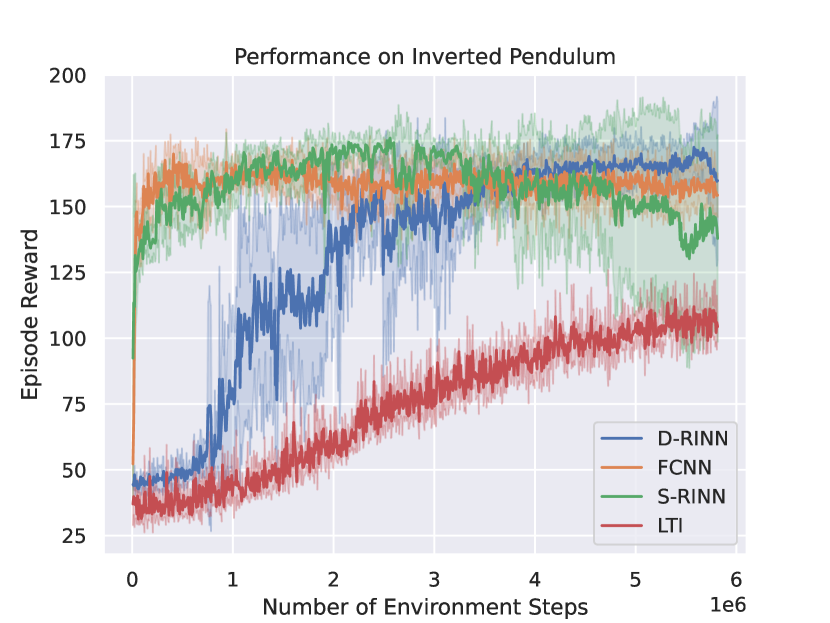
Figure 4: Evaluation reward vs. number of training environment steps for the Dissipative Recurrent Implicit Neural Network (D-RINN, our method), Fully Connected Neural Network (FCNN), Standard RINN (S-RINN), and linear time-invariant (LTI) controllers on the inverted pendulum. The solid line represents the mean, and the shaded region represents 1 standard deviation. The reward is upper bounded by 201, and lower bounded by 0. Higher reward indicates lower control effort. The Dissipative RINN and LTI controllers both guarantee stability of the inverted pendulum.

We compare the Dissipative RINN with the following controllers:

• Standard RINN: This model has the same state and nonlinearity sizes as the Dissipative RINN. After each training step, $\|D_{kvw}\|_{\infty}$ is reduced to be less than 1 to guarantee well-posedness [4]. We use a learning rate of $10^{-3}$ for this model.

• LTI: This model has the same state size as the Dissipative RINN. It is initialized using the same method as used for the Dissipative RINN, and is trained using Algorithm 1, with the only difference being that the $\hat{\theta}$ and $\theta$ projection steps are restricted so that they correspond only to LTI controllers. We use the same $t_{RS}$ value in (25) as for the Dissipative RINN. We use a learning rate of $10^{-2}$ for this model since it gives faster convergence without a performance penalty.

• Fully Connected Neural Network: The fully connected neural network has two hidden layers, both with size 19, to give a total number of parameters roughly the same as the two RINN controllers. We use a learning rate of $10^{-4}$ for this model.

Figure 4 plots the performance of the four controllers vs. the number of training environment steps sampled. Each controller is trained five times, and the mean and standard deviations of the reward of these runs is plotted. The Standard RINN controller reaches the highest reward of the four models, with the fully connected neural network achieving similar reward. The Dissipative RINN and LTI controllers both guarantee closed-loop stability, and due to a common initialization method, start with similar reward. However the Dissipative RINN ultimately reaches reward comparable to the Standard RINN and fully connected neural network, while the LTI controller reward stabilizes at a level below the neural network controllers. Thus, in this experiment, our Dissipative RINN controller achieves both the performance of an unconstrained neural network controller and the stability guarantees of a standard LTI controller.

5.2 Flexible Rod on a Cart

In this example we consider a flexible rod on a cart (see Figure 5 for a diagram). This consists of a movable cart with a metal rod fixed on top and a mass at the top of the rod. Unlike the typical cart pole setup, there is no joint at the base of the rod. However, the rod is flexible, so the horizontal position of the top and bottom of the rod can differ. Training is conducted with the higher-fidelity flexible model (26) below, but $L_{2}$ gain constraints (where applied) are formulated with respect to a simplified model where the rod is rigid, allowing some uncertainty. We compare the Dissipative RINN, Standard RINN, LTI, and fully connected neural network controllers on a reward function that rewards a combination of the state of the flexible rod on a cart being close to 0 and of the control effort being small.

Figure 5: Diagram of the flexible rod on a cart.

The true dynamics, with the flexible rod, are taken as:

$$\dot{\boldsymbol{x}}_{\boldsymbol{f}}(t) =\begin{bmatrix}0&I\\ -M^{-1}K&-M^{-1}B\end{bmatrix}\boldsymbol{x_{f}}(t)+\begin{bmatrix}0\\ M^{-1}\begin{bmatrix}1\\ 0\end{bmatrix}\end{bmatrix}\boldsymbol{u}(t)$$ (26)

$$\boldsymbol{y}(t) =\begin{bmatrix}1&1&0&0\end{bmatrix}\boldsymbol{x_{f}}(t)$$

$$M =\begin{bmatrix}m_{b}+m_{r}+\rho L&m_{t}+\frac{\rho L}{3}\\ m_{t}+\frac{\rho L}{3}&m_{t}+\frac{\rho L}{5}\end{bmatrix}$$

$$K =\begin{bmatrix}0&0\\ 0&\frac{4EI}{L^{3}}\end{bmatrix}$$

$$B =\begin{bmatrix}0&0\\ 0&0.9\end{bmatrix}$$

where $x_{f}=\begin{bmatrix}x_{b}&h&\dot{x_{b}}&\dot{h}\end{bmatrix}^{\top}\in\mathbb{R}^{4}$ is the state of the flexible rod on a cart, $x_{b}$ is the position of the base of the rod, $h$ is the horizontal deviation of the top of the rod from the base of the rod, $m_{b}=1$ kg is the mass of the base, $m_{t}=0.1$ kg is the mass of an object at the top of the rod, $L=1$ m is the length of the rod, $\rho=0.1$ N/m is the mass density of the rod, $r=10^{-2}$ m is the radius of the rod cross-section, $E=200\cdot 10^{-9}$ GPa is the Young’s modulus of steel, and $I=\frac{\pi}{4}r^{4}$ m⁴ is the area second moment of inertia. The output $y$ represents the measurement of the position of the tip of the rod.

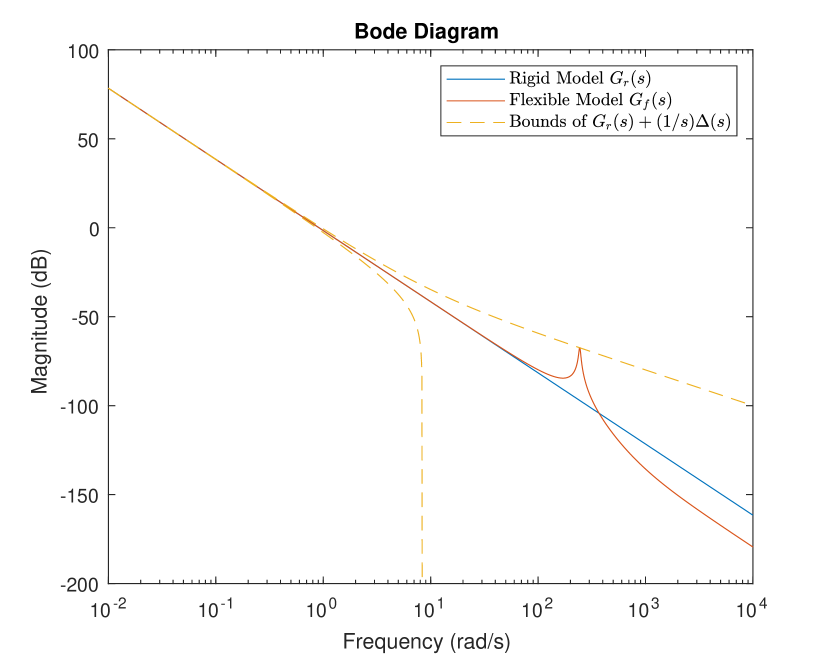
Figure 6: Bode magnitude plot, for the flexible rod on a cart, of the rigid model, the flexible model, and the bounds on the uncertain rigid model. The flexible model lies within the bounds of the uncertain rigid model.

The Dissipative RINN and LTI controllers are designed with respect to the following uncertain rigid model:

$$\dot{\boldsymbol{x}}_{\boldsymbol{r}}(t) =\begin{bmatrix}0&1\\ 0&0\end{bmatrix}\boldsymbol{x_{r}}(t)$$

$$\hphantom{=}+\begin{bmatrix}0\\ \frac{1}{m_{b}+m_{r}+\rho L}\end{bmatrix}(\boldsymbol{u}(t)+\boldsymbol{d}(t))+\begin{bmatrix}1\\ 0\end{bmatrix}\boldsymbol{w}(t)$$

$$\boldsymbol{w}(t) =\Delta(\boldsymbol{u}+\boldsymbol{d})(t)$$

$$\boldsymbol{y}(t) =\boldsymbol{x_{b}}(t)$$

$$\boldsymbol{e}(t) =\boldsymbol{x_{r}}(t),$$

where $x_{r}=\begin{bmatrix}x_{b}&\dot{x}_{b}\end{bmatrix}^{\top}$ and $\|\Delta\|\leq 0.1$. The norm-bounded $\Delta$ block is used to represent uncertainty in the dynamical model. If the rigid model with no uncertainty ($\Delta=0$) has a transfer function from input $\boldsymbol{u+d}$ to output $\boldsymbol{y}$ of $G_{r}(s)$, then this uncertain model represents transfer functions of the form $G_{r}(s)+\frac{1}{s}\Delta(s)$ where $\|\Delta(s)\|\leq 0.1$. The value of $0.1$ is chosen such that this set includes $G_{f}(s)$, the transfer function from input to output of the flexible model. This ensures that a controller designed with closed-loop properties for this uncertain rigid model will satisfy the same properties for the flexible model. See Figure 6 for a Bode magnitude plot of $G_{r}(s)$, $G_{f}(s)$, and the bounds on $G_{r}(s)+\frac{1}{s}\Delta(s)$.

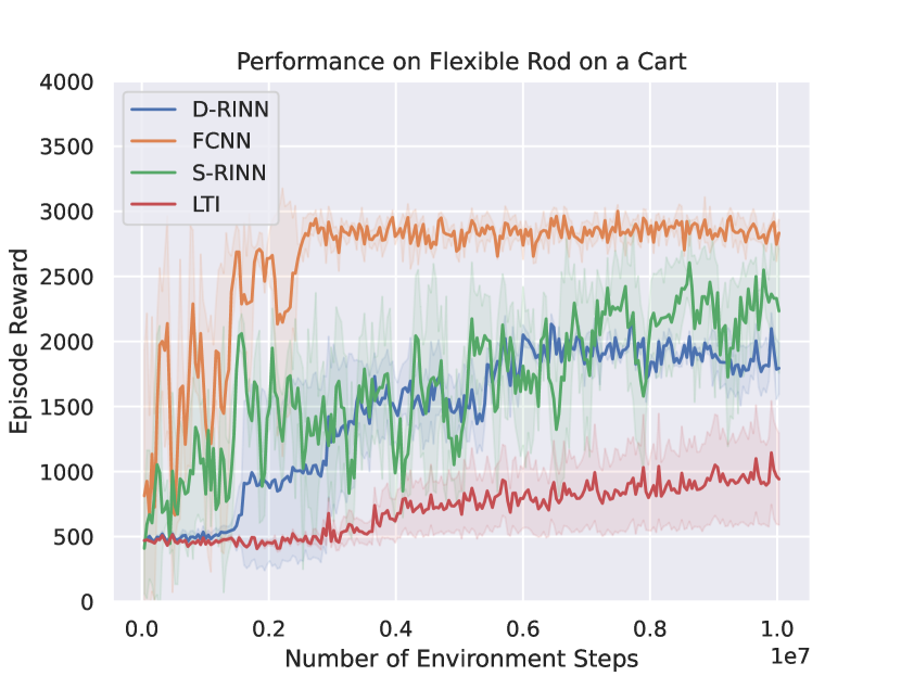
Figure 7: Evaluation reward vs. number of training environment steps for the Dissipative Recurrent Implicit Neural Network (D-RINN, our method), Fully Connected Neural Network (FCNN), Standard RINN (S-RINN), and linear time-invariant (LTI) controllers on the flexible rod on a cart. The solid line represents the mean, and the shaded region represents 1 standard deviation. The reward is upper bounded by 4000, and lower bounded by 0. Higher reward indicates a combination of lower control effort and the state of the flexible rod on a cart being close to 0. The Dissipative RINN and LTI controllers both guarantee an $L_{2}$ gain of at most 0.99 from a disturbance in the control input to the state for the uncertain rigid model.

The norm-bound on $\Delta$ is characterized with a quadratic constraint of $M_{\Delta_{p}}=5\begin{bmatrix}0.1^{2}&0\\ 0&-1\end{bmatrix}$. The scaling factor of 5 is the $\lambda$ value used in Lemma 1. This affects the feasible set, but not the norm-bound. The supply rate in synthesizing these controllers is set to $0.5\begin{bmatrix}0.99&0\\ 0&-I\end{bmatrix}$, constraining the $L_{2}$ gain from disturbance into the control input to the rigid model state being less than or equal to 0.99. Scaling the supply rate does not change the $L_{2}$ gain property. We use a $t_{RS}$ value of 1.0 (in (25)) and a backoff factor of $\beta=1.05$ to tune suboptimality of the projection (as described in Section 4.3).

We simulate the controllers and plant with a time step of $0.001$ seconds, and train with a time horizon of 2 seconds. The reward for each time step is $\exp(-\|x_{f}\|^{2})+\exp(-u^{2})$. Initial conditions are sampled uniformly at random with $x_{b}\in[-1,1]$ m, $h\in[-0.44,0.44]$ m, $\dot{x}_{b}\in[-0.25,0.25]$ m/s, and $\dot{h}\in[-2,2]$ m/s. The control input is limited (saturated) to remain in the interval $[-20,20]$.

We experiment with a Dissipative RINN with a state size, $n_{k}$, of 2, and a nonlinearity size, $n_{\phi}$, of 16. The controller is initialized with an LTI controller as described in Section 5.1. We use a learning rate of $10^{-5}$ for this model to improve stability during training. We compare the Dissipative RINN with the following controllers:

• Standard RINN: This model has the same state and nonlinearity sizes as the Dissipative RINN. After each training step, $\|D_{kvw}\|_{\infty}$ is reduced to be less than 1 to guarantee well-posedness [4]. We use a learning rate of $5\cdot 10^{-5}$ for this model.

• LTI: This model has the same state size as the Dissipative RINN. It is initialized using the same method as used for the Dissipative RINN, and is trained as described in Section 5.1. We use a learning rate of $5\cdot 10^{-5}$ for this model.

• Fully Connected Neural Network: The fully connected neural network has two hidden layers, both with size 19, to give a total number of parameters roughly the same as the two RINN controllers. We use a learning rate of $5\cdot 10^{-5}$ for this model.

The results of performance vs. number of training environment steps sampled is plotted in Figure 7, with each controller trained thrice and the mean and standard deviations taken. The fully connected feed forward neural network achieves the highest reward. The Standard RINN achieves the next highest, closely followed by the Dissipative RINN. The LTI controller achieves the least reward. In this example, the Dissipative RINN demonstrates a significant performance advantage over the LTI controller, while maintaining the same robustness guarantee, but does not quite achieve the performance of the unconstrained feed forward neural network.

6 Conclusion

In this paper, we derived a convex condition for certifying dissipativity of a feedback system of an uncertain LTI plant and a neural network controller. The derivation of this condition leverages implicit neural networks and integral quadratic constraints to model the neural network controller and the plant in the same form. We used this condition in a method to train neural network controllers that provide closed-loop guarantees. We applied this method to an inverted pendulum model to train a stabilizing controller to use minimal control effort, and to a flexible rod on a cart model to train a controller guaranteeing a closed-loop $L_{2}$ gain upper bound to stabilize the system with small control effort. These experiments showed that the neural network controller with formal closed-loop guarantees achieved significantly higher performance than that of an LTI controller and closer to that of an unconstrained neural network controller.

Future directions of research include reducing conservatism of the over-approximation of the neural network nonlinearity, improving the scalability of this LMI-based approach, improving the stability of training RINNs, and accelerating training of RINNs.

Appendix A Expansion of Extended and Transformed System

This section includes the expansion of the system that is the result of augmenting an uncertain LTI system with the filters corresponding to the dynamic IQC as described in Section 3.2. The definitions of the tilde variables are as follows.

$$\begin{gathered}\begin{bmatrix}\tilde{A}&\tilde{B}_{w}&\tilde{B}_{d}\\ \tilde{C}_{v}&\tilde{D}_{vw}&\tilde{D}_{vd}\\ \tilde{C}_{e}&\tilde{D}_{ew}&\tilde{D}_{ed}\end{bmatrix}=\\ \left[\begin{array}[]{ccc|c|c}A&0&0&B_{w}&B_{d}\\ B_{\psi_{1}}C_{v}&A_{\psi_{1}}&0&B_{\psi_{1}}D_{vw}&B_{\psi_{1}}D_{vd}\\ 0&0&A_{\psi_{2}}&B_{\psi_{2}}&0\\ \hline\cr D_{\psi_{1}}C_{v}&C_{\psi_{1}}&0&D_{\psi_{1}}D_{vw}&D_{\psi_{1}}D_{vd}\\ \hline\cr C_{e}&0&0&D_{ew}&D_{ed}\end{array}\right]\end{gathered}$$

Appendix B Expansion of Closed-Loop System

This section includes the expansion of the feedback system of plant and controller, described in Section 4.

$$A =\begin{bmatrix}A_{p}+B_{pu}D_{kuy}C_{py}&B_{pu}C_{ku}\\ B_{ky}C_{py}&A_{k}\end{bmatrix}$$

$$B_{w} =\begin{bmatrix}B_{pw}+B_{pu}D_{kuy}D_{pyw}&B_{pu}D_{kuw}\\ B_{ky}D_{pyw}&B_{kw}\end{bmatrix}$$

$$B_{d} =\begin{bmatrix}B_{pd}+B_{pu}D_{kuy}D_{pyd}\\ B_{ky}D_{pyd}\end{bmatrix}$$

$$C_{v} =\begin{bmatrix}C_{pv}+D_{pvu}D_{kuy}C_{py}&D_{pvu}C_{ku}\\ D_{kvy}C_{py}&C_{kv}\end{bmatrix}$$

$$D_{vw} =\begin{bmatrix}D_{pvw}+D_{pvu}D_{kuy}D_{pyw}&D_{pvu}D_{kuw}\\ D_{kvy}D_{pyw}&D_{kvw}\end{bmatrix}$$

$$D_{vd} =\begin{bmatrix}D_{pvd}+D_{pvu}D_{kuy}D_{pyd}\\ D_{kvy}D_{pyd}\end{bmatrix}$$

$$C_{e} =\begin{bmatrix}C_{pe}+D_{peu}D_{kuy}C_{py}&D_{peu}C_{ku}\end{bmatrix}$$

$$D_{ew} =\begin{bmatrix}D_{pew}+D_{peu}D_{kuy}D_{pyw}&D_{peu}D_{kuw}\end{bmatrix}$$

$$D_{ed} =D_{ped}+D_{peu}D_{kuy}D_{pyd}$$

References

- [1] Shaojie Bai, J. Zico Kolter, and Vladlen Koltun. Deep equilibrium models. In Advances in Neural Information Processing Systems, volume 32. Curran Associates, Inc., 2019.
- [2] Stephen P. Boyd, editor. Linear Matrix Inequalities in System and Control Theory. Number vol. 15 in SIAM Studies in Applied Mathematics. Society for Industrial and Applied Mathematics, 1994.
- [3] Frank M. Callier and Charles A. Desoer. Linear System Theory. Springer Texts in Electrical Engineering. Springer, 1991.
- [4] Laurent El Ghaoui, Fangda Gu, Bertrand Travacca, Armin Askari, and Alicia Tsai. Implicit deep learning. SIAM Journal on Mathematics of Data Science, 3(3):930–958, 2021. Publisher: Society for Industrial and Applied Mathematics.
- [5] Mahyar Fazlyab, Manfred Morari, and George J. Pappas. Safety verification and robustness analysis of neural networks via quadratic constraints and semidefinite programming. IEEE Transactions on Automatic Control, 67(1):1–15, 2022.
- [6] Mahyar Fazlyab, Alexander Robey, Hamed Hassani, Manfred Morari, and George Pappas. Efficient and accurate estimation of Lipschitz constants for deep neural networks. In Advances in Neural Information Processing Systems, volume 32. Curran Associates, Inc., 2019.
- [7] Fangda Gu, He Yin, Laurent El Ghaoui, Murat Arcak, Peter Seiler, and Ming Jin. Recurrent neural network controllers synthesis with stability guarantees for partially observed systems. Proceedings of the AAAI Conference on Artificial Intelligence, 36(5):5385–5394, 2022.
- [8] Navid Hashemi, Justin Ruths, and Mahyar Fazlyab. Certifying incremental quadratic constraints for neural networks via convex optimization. In Proceedings of the 3rd Conference on Learning for Dynamics and Control, pages 842–853. PMLR, 2021.
- [9] Neelay Junnarkar, He Yin, Fangda Gu, Murat Arcak, and Peter Seiler. Synthesis of stabilizing recurrent equilibrium network controllers. In 2022 IEEE 61st Conference on Decision and Control (CDC), pages 7449–7454, 2022. ISSN: 2576-2370.
- [10] Timothy P. Lillicrap, Jonathan J. Hunt, Alexander Pritzel, Nicolas Heess, Tom Erez, Yuval Tassa, David Silver, and Daan Wierstra. Continuous control with deep reinforcement learning. In Yoshua Bengio and Yann LeCun, editors, 4th International Conference on Learning Representations, ICLR 2016, San Juan, Puerto Rico, May 2-4, 2016, Conference Track Proceedings, 2016.
- [11] A. Megretski and A. Rantzer. System analysis via integral quadratic constraints. IEEE Transactions on Automatic Control, 42(6):819–830, 1997.
- [12] Patricia Pauli, Niklas Funcke, Dennis Gramlich, Mohamed Amine Msalmi, and Frank Allgöwer. Neural network training under semidefinite constraints. In 2022 IEEE 61st Conference on Decision and Control (CDC), pages 2731–2736, 2022. ISSN: 2576-2370.
- [13] Patricia Pauli, Dennis Gramlich, Julian Berberich, and Frank Allgöwer. Linear systems with neural network nonlinearities: Improved stability analysis via acausal Zames-Falb multipliers. In 2021 60th IEEE Conference on Decision and Control (CDC), pages 3611–3618, 2021.
- [14] Patricia Pauli, Anne Koch, Julian Berberich, Paul Kohler, and Frank Allgöwer. Training robust neural networks using Lipschitz bounds. IEEE Control Systems Letters, 6:121–126, 2022.
- [15] Max Revay, Ruigang Wang, and Ian R. Manchester. Recurrent equilibrium networks: Flexible dynamic models with guaranteed stability and robustness. IEEE Transactions on Automatic Control, pages 1–16, 2023.
- [16] Carsten Scherer, Pascal Gahinet, and Mahmoud Chilali. Multiobjective output-feedback control via LMI optimization. IEEE Transactions on Automatic Control, 42(7):896–911, 1997.
- [17] Carsten W. Scherer. Dissipativity and Integral Quadratic Constraints: Tailored Computational Robustness Tests for Complex Interconnections. 42(3):115–139.
- [18] Peter Seiler. Stability analysis with dissipation inequalities and integral quadratic constraints. IEEE Transactions on Automatic Control, 60(6):1704–1709, 2015. Conference Name: IEEE Transactions on Automatic Control.
- [19] Richard S. Sutton and Andrew Barto. Reinforcement Learning: An Introduction. Adaptive Computation and Machine Learning. The MIT Press, second edition, 2020.
- [20] Elise van der Pol, Daniel Worrall, Herke van Hoof, Frans Oliehoek, and Max Welling. MDP homomorphic networks: Group symmetries in reinforcement learning. In H. Larochelle, M. Ranzato, R. Hadsell, M.F. Balcan, and H. Lin, editors, Advances in Neural Information Processing Systems, volume 33, pages 4199–4210. Curran Associates, Inc., 2020.
- [21] Joost Veenman and Carsten W. Scherer. IQC-Synthesis with general dynamic multipliers. International Journal of Robust and Nonlinear Control, 24(17):3027–3056, 2014.
- [22] Joost Veenman, Carsten W. Scherer, and Hakan Köroğlu. Robust stability and performance analysis based on integral quadratic constraints. European Journal of Control, 31:1–32, 2016.
- [23] Dian Wang, Robin Walters, and Robert Platt. SO-2 Equivariant Reinforcement Learning. In International Conference on Learning Representations, 2022.
- [24] Ruigang Wang, Nicholas H. Barbara, Max Revay, and Ian R. Manchester. Learning over all stabilizing nonlinear controllers for a partially-observed linear system. IEEE Control Systems Letters, 7:91–96, 2023.
- [25] Shu Wang, Harald Pfifer, and Peter Seiler. Robust synthesis for linear parameter varying systems using integral quadratic constraints. Automatica, 68:111–118, 2016.
- [26] Jan C. Willems. Dissipative dynamical systems part I: General theory. Archive for Rational Mechanics and Analysis, 45(5):321–351, 1972.
- [27] Jan C. Willems. Dissipative dynamical systems part II: Linear systems with quadratic supply rates. Archive for Rational Mechanics and Analysis, 45(5):352–393, 1972.
- [28] He Yin, Peter Seiler, and Murat Arcak. Stability analysis using quadratic constraints for systems with neural network controllers. IEEE Transactions on Automatic Control, 67(4):1980–1987, 2022.