Gradient Networks

Abstract

Directly parameterizing and learning gradients of functions has widespread significance, with specific applications in optimization, generative modeling, and optimal transport. This paper introduces gradient networks (GradNets): novel neural network architectures that parameterize gradients of various function classes. GradNets exhibit specialized architectural constraints that ensure correspondence to gradient functions. We provide a comprehensive GradNet design framework that includes methods for transforming GradNets into monotone gradient networks (mGradNets), which are guaranteed to represent gradients of convex functions. We establish the approximation capabilities of the proposed GradNet and mGradNet. Our results demonstrate that these networks universally approximate the gradients of (convex) functions. Furthermore, these networks can be customized to correspond to specific spaces of (monotone) gradient functions, including gradients of transformed sums of (convex) ridge functions. Our analysis leads to two distinct GradNet architectures, GradNet-C and GradNet-M, and we describe the corresponding monotone versions, mGradNet-C and mGradNet-M. Our empirical results show that these architectures offer efficient parameterizations and outperform popular methods in gradient field learning tasks.

1 Introduction

Deep neural networks have the ability to parameterize and learn complicated, high-dimensional functions. Considerable attention has been devoted to training deep neural networks to achieve state of the art performance on numerous tasks spanning computer vision [1], natural language processing [2], and reinforcement learning [3]. The neural networks used in these tasks are commonly unconstrained and effectively parameterize the space of all functions. However, many applications demand the learned function to exhibit specific properties. Such applications thus motivate design of neural networks that exclusively correspond to specific function classes – a problem that has seldom been studied. Constraining neural networks to be in a particular function class can not only enhance interpretability, but can also lead to theoretical performance guarantees essential for deploying learned models in safety-critical applications.

In particular, the ability to parameterize neural networks precisely corresponding to gradients of functions has broad significance across several disciplines in science and engineering. For example, in physics, one often wishes to characterize the gradient field of a potential function, such as the temperature gradient over a surface, from a finite set of measurements. Score-based generative models are another application of learning gradient functions where neural networks are trained to represent the score function, $\nabla_{\boldsymbol{x}}p(\boldsymbol{x})$, of an unknown probability distribution $p(\boldsymbol{x})$ [4, 5]. Such score-based methods can be applied to tasks including 3D shape [6] and molecule [7] generation.

Learning gradients of convex functions holds particular significance in the theory of optimal transport. Brenier’s theorem states that the unique solution to the Monge problem with Euclidean cost is given by the gradient of a convex function [8, 9]. The theorem highlights the utility of gradients of convex functions in density estimation applications and further warrants their use in generative models like normalizing flows [10]. Applications of learned gradients of convex functions also extend to gradient-based optimization. Optimization routines can incorporate a learned gradient map to characterize a set of iterative updates that map a given input to a desired output. In particular, gradients of convex functions can be used to define gradients of regularization terms in optimization algorithms. Such methods have become popular especially for addressing ill-posed inverse problems and yield strong theoretical guarantees [11, 12].

Contributions: We propose gradient networks (GradNets) for directly parameterizing gradients of arbitrary functions. We adapt GradNets to monotone gradient networks (mGradNets) that correspond to gradients of convex functions. Our proposed neural network architectures directly model the gradient function $\nabla F$ without first modeling the underlying potential function $F$. We analyze the expressivity of our proposed GradNet and mGradNet networks and prove that they are respectively universal approximators of gradients of general functions and gradients of convex functions. We also describe methods by which these networks can be modified to represent popular subsets of these function classes, including gradients of sums of (convex) ridge functions and their (convexity-preserving) transformations. In our gradient field approximation experiments, we compare to existing methods and find that our architectures achieve significantly lower mean squared error.

Paper Organization: We first review existing methods for representing gradients of functions in Sec. 2. We then present gradient networks (GradNets) for learning gradients of arbitrary functions in Sec. 3 and show how they can be modified to represent gradients of convex functions. These modified GradNets are called monotone gradient networks (mGradNets) and are described in Sec. 4. We analyze the expressivity of our proposed GradNets and mGradNets in Sec. 5 and demonstrate methods for composing GradNets and mGradNets to learn gradients of specific function classes described in Fig. 1. We present architectural enhancements in Sec. 6 that empirically yield efficient parameterizations for gradient functions. Finally, in Sec. 7, we evaluate the efficacy of our proposed models on a series of gradient field learning tasks.

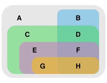
Figure 1: Relationships between relevant function classes: A) all functions, B) monotone functions, C) gradient functions, D) monotone gradient functions, E) gradients of transformed sums of ridges, F) gradients of transformed sums of convex ridges, G) gradients of sums of ridges, H) gradients of sums of convex ridges.

Notation: $\boldsymbol{w}$ and $\boldsymbol{W}$ respectively denote vectors and matrices. $\nabla F(\boldsymbol{x})$ is the gradient of a scalar-valued function $F$ at a point $\boldsymbol{x}$ and is a vector-valued function. $\boldsymbol{H}_{F}(\boldsymbol{x})$ is the Hessian of $F$ at $\boldsymbol{x}$, the matrix of second-order partial derivatives. When a function $f$ is vector-valued, $\boldsymbol{J}_{f}(\boldsymbol{x})$ denotes the Jacobian of $f$ at $\boldsymbol{x}$, the matrix of partial derivatives. $\boldsymbol{A}\succeq 0$ indicates $\boldsymbol{A}$ is symmetric positive semidefinite (PSD). $\mathrm{diag}(\cdot)$ is the vector-to-diagonal-matrix operator. $C(\mathcal{D})$ and $C^{k}(\mathcal{D})$ respectively denote the space of continuous and $k$-times continuously differentiable functions that map from domain $\mathcal{D}$ to the real numbers $\mathbb{R}$. $C^{k}_{\times}(\mathcal{D})$ are the convex functions in $C^{k}(\mathcal{D})$. $\odot$ is the Hadamard (entrywise) vector product and $\|\cdot\|$ denotes the $\ell_{2}$ norm for vectors and the spectral norm for matrices.

2 Related Work

The majority of existing work uses standard neural networks to directly model the gradient of a function [13, 14, 15]. While these methods demonstrate satisfactory empirical performance, they lack theoretical justification and are often considered heuristic approaches. It is not guaranteed, and in fact highly unlikely, that an arbitrary neural network with matching input and output dimension corresponds to the gradient of a scalar-valued function. More formally, let $\mathcal{F}$ be such that each function $F\in\mathcal{F}$ is the gradient of a scalar-valued function. Given $F\in\mathcal{F}$, standard neural network architectures, e.g., multilayer perceptrons (MLPs) and convolutional neural networks (CNNs), with nonpolynomial activations can be used to approximate $F$. However, these architectures offer no guarantee that the learned function $\widehat{F}$ is itself in $\mathcal{F}$. In contrast, the methods and network architectures discussed in this paper ensure that the approximator $\widehat{F}$ is always a member of $\mathcal{F}$, thereby enhancing interpretability of the network and enabling robust theoretical guarantees in practice.

Rather than directly approximating the gradient of a function using a standard neural network, an attractive, indirect approach may be to first parameterize and learn the underlying scalar potential function using a standard neural network. Subsequently differentiating the network with respect to its input extracts a gradient function that is guaranteed to have an antiderivative. It is worth noting that this approach is theoretically flawed because, in general, closely approximating a target function $F$ with a function $G$ does not guarantee that $\nabla G$ closely approximates $\nabla F$ [16]. Empirical evidence in [17] confirms this fact when the approximating functions are neural networks. An alternative approach is to directly train the gradient map of a standard neural network. For instance, ref. [18] employs automatic differentiation on an MLP to obtain a gradient network architecture. Nevertheless, these approaches often exhibit ill-behaved product structures [19] and, by the Runge phenomena [20], optimizing their parameters becomes cumbersome as the input dimension grows [21].

The literature on parameterizing and learning the gradients of convex functions (monotone gradient functions) includes various approaches. Input Convex Neural Networks (ICNN) [22] parameterize only convex functions by requiring positive weight matrices and convex, monotonically increasing elementwise activation functions. Refs. [23, 24, 10] use a computationally-expensive, two-step approach of first computing a convex function with an ICNN and then differentiating the network with respect to its input (via backpropagation) to evaluate its gradient. While [10] provides theoretical justification for this approach, in practice the ICNN’s architectural restrictions still result in training difficulties that have been well-documented [21, 25]. Our approach in this paper avoids these challenges and bypasses the two-step process by directly characterizing and learning the gradient.

Input Convex Gradient Networks (ICGNs) [21] use a different two-step process to learn monotone gradient functions. ICGNs first train a restricted neural network to approximate a factor of the positive semidefinite (PSD) Jacobian of a monotone gradient function, which corresponds to the PSD Hessian of a convex function. As detailed in [21], the only neural network architecture currently known to satisfy the partial differential equation constraint are perceptrons without any hidden layers. Nevertheless, the monotone gradient function is obtained by numerically integrating the Gram matrix corresponding to the neural network’s output matrix. Numerical integration additionally faces severe computational challenges for modern, high-dimensional problems [26].

A single hidden layer neural network with learnable spline activation functions is proposed in [11] to directly parameterize the gradient of a convex function. The elementwise spline activations enable fast training in practice, but require additional hyperparameter tuning and training procedures beyond standard backpropagation. The spline activations limit the representation power of the network, restricting it to approximate the gradient of a sum of convex ridge functions: $f(\boldsymbol{x})=\sum_{i=1}^{n}\psi_{i}(\boldsymbol{w}_{i}^{\top}\boldsymbol{x})$, where $\psi_{i}:\mathbb{R}\to\mathbb{R}$ is convex and continuously differentiable. Note the class of functions expressible as a sum of convex ridge is limited and does not include several common convex functions, including:

$$\text{Max}: \max\{\boldsymbol{x}_{1},\boldsymbol{x}_{2},\dots,\boldsymbol{x}_{n}\}$$ (1)

$$\text{Infinity Norm}: \max\{|\boldsymbol{x}_{1}|,|\boldsymbol{x}_{2}|,\dots,|\boldsymbol{x}_{n}|\}$$ (2)

$$\text{Exponential Product}: \exp\left(\sum_{i=1}^{n}\boldsymbol{x}_{i}\right)$$ (3)

$$\text{LogSumExp}: \log\left[\sum_{i=1}^{n}\exp(\boldsymbol{x}_{i})\right]$$ (4)

In contrast to the approach in [11], the architectures we propose can be trained with standard backpropagation to approximate the gradient of any function. Our further refinements in Sections 4,5.2, and 5.3 respectively enable approximating the gradient of any convex function, any sum of (convex) ridges, and transformed sums of (convex) ridges. The framework we establish for the design of such networks is general, and notably, the network in [11] emerges as a specific instance of the methods we describe.

3 Gradient Networks (GradNet)

In this section, we introduce gradient networks (GradNet) for parameterizing and learning gradients of twice continuously differentiable functions. We first state necessary and sufficient conditions for a neural network to be a GradNet. We then discuss various approaches for constructing a GradNet.

Definition 1.

(GradNet) A neural network $f$ is a gradient network (GradNet) if $f=\nabla F$ for some $F\in C^{2}\left(\mathbb{R}^{d}\right)$.

By Def. 1, differentiating a neural network that parameterizes a function $F\in C^{2}(\mathbb{R}^{d})$ yields a GradNet. However, for the reasons discussed in Sec. 2, this paper focuses on directly parameterizing and learning $\nabla F$ (without first characterizing $F$). Our design of GradNets is inspired by a theorem credited to Clairaut, Schwarz, and Young, among others.

Theorem 1 (Clairaut’s Theorem on symmetry of second derivatives [27]).

If $F\in C^{2}(\mathbb{R}^{d})$, then the Hessian of $F$ is symmetric everywhere, i.e., $\forall\boldsymbol{x}\in\mathbb{R}^{d},\;\boldsymbol{H}_{F}(\boldsymbol{x})=\boldsymbol{H}_{F}(\boldsymbol{x})^{\top}$.

Recall that the Hessian of a function is the transposed Jacobian of its gradient map: $\boldsymbol{H}_{F}=\boldsymbol{J}_{\nabla F}^{\top}$. Thus, Thm. 1 implies that the Jacobian of a GradNet must be everywhere symmetric. However, note that Thm. 1 does not ensure existence of an antiderivative for a function with symmetric Jacobian. The next theorem uses the Poincaré Lemma[28] to guarantee existence of an antiderivative and show that the symmetric Jacobian condition is both necessary and sufficient.

Theorem 2.

A differentiable function $f:\mathbb{R}^{d}\to\mathbb{R}^{d}$ is a GradNet if and only if its Jacobian is symmetric everywhere, i.e., $\forall\boldsymbol{x}\in\mathbb{R}^{d}\;\boldsymbol{J}_{f}(\boldsymbol{x})=\boldsymbol{J}_{f}(\boldsymbol{x})^{\top}$.

Proof.

($\rightarrow$): By Def. 1, we have $\boldsymbol{J}^{\top}_{f}=\boldsymbol{J}^{\top}_{\nabla F}=\boldsymbol{H}_{F}$, which must be symmetric by Thm. 1. ($\leftarrow$): The proof leverages the theory of differential forms and the Poincaré lemma (see [28] for details). We express the smooth (differentiable) vector field $f$ as its corresponding 1-form, $f=\sum_{i=1}^{n}f_{i}dx^{i}$, where $f_{i}(\boldsymbol{x})=[f(\boldsymbol{x})]_{i}$. The exterior derivative [28] of $f$ is:

$$df =\sum_{i=1}^{n}d(f_{i})\wedge dx^{i}=\sum_{i=1}^{n}\sum_{j=1}^{n}\frac{\partial f_{i}}{\partial x^{j}}dx^{j}\wedge dx^{i}$$ (5)

where $\wedge$ denotes the wedge product. Since $dx^{i}\wedge dx^{i}=0$, the terms with $i=j$ sum to $0$. For the terms with $i\neq j$,

$$\frac{\partial f_{i}}{\partial x^{j}}dx^{j}\wedge dx^{i}=-\frac{\partial f_{i}}{\partial x^{j}}dx^{i}\wedge dx^{j}=-\frac{\partial f_{j}}{\partial x^{i}}dx^{i}\wedge dx^{j}$$ (6)

where the first equality follows by the wedge product’s antisymmetric property and the second equality follows by symmetry of $\boldsymbol{J}_{f}$. Therefore, terms in (5) with $i\neq j$ also sum to 0. This means $df=0$ and $f$ is a closed 1-form. The Poincaré lemma states that every closed 1-form on a simply connected open subset of $\mathbb{R}^{d}$ is exact, that is, there exists a 0-form $F$ such that $dF=\sum_{i=1}^{n}\frac{\partial F}{\partial x^{i}}dx^{i}=f$. Converting the 1-form $f$ to its associated vector field, we get $f=\begin{bmatrix}\frac{\partial F}{\partial x_{1}}&\dots&\frac{\partial F}{\partial x_{n}}\end{bmatrix}^{\top}=\nabla F$ and thus $f$ is a GradNet. ∎

Thus, a neural network is a GradNet if and only if its Jacobian, with respect to the input, is everywhere symmetric. Since symmetry of the Jacobian is preserved under linear combinations, Thm. 2 implies the following:

Corollary 2.1.

A linear combination of GradNets is also a GradNet.

Traditional feedforward neural networks consist of an affine transformation in the first layer followed by successive alternating nonlinear and affine transformations in subsequent layers. By Thm. 2, composing these layers to construct a GradNet requires ensuring that the network’s Jacobian is everywhere symmetric. The next corollary specifies a composition that satisfies this condition and produces a GradNet.

Corollary 2.2.

Let $f:\mathbb{R}^{d}\to\mathbb{R}^{m}$ be the affine function $f(\boldsymbol{x})=\boldsymbol{W}\boldsymbol{x}+\boldsymbol{b}$ and $g:\mathbb{R}^{m}\to\mathbb{R}^{d}$ be differentiable. If $\forall\boldsymbol{x}\in\mathbb{R}^{d},$ $\boldsymbol{J}_{g}(\boldsymbol{x})=\boldsymbol{W}^{\top}\boldsymbol{M}(\boldsymbol{x})$, where $\boldsymbol{M}(\boldsymbol{x})$ is symmetric everywhere, then the composition $g\circ f$ is a GradNet.

Proof.

$\boldsymbol{J}_{g\circ f}(\boldsymbol{x})=\boldsymbol{J}_{g}(f(\boldsymbol{x}))\boldsymbol{J}_{f}(\boldsymbol{x})=\boldsymbol{W}^{\top}\boldsymbol{M}(f(\boldsymbol{x}))\boldsymbol{W}$ and is symmetric everywhere. By Thm. 2, $g\circ f$ is a GradNet. ∎

Cor. 2.2 is a sufficient condition that provides a practical method for designing subsequent layers that ensure symmetry of $\boldsymbol{J}_{g}(\boldsymbol{x})\boldsymbol{W}$ without placing additional restrictions on $\boldsymbol{W}$. We next use it to readily specify a single hidden layer GradNet.

Proposition 2.1.

The single hidden layer neural network

$$\boldsymbol{W}^{\top}\sigma(\boldsymbol{W}\boldsymbol{x}+\boldsymbol{a})+\boldsymbol{b}$$ (7)

is a GradNet if the differentiable activation $\sigma:\mathbb{R}^{m}\to\mathbb{R}^{m}$ has a symmetric Jacobian $\boldsymbol{J}_{\sigma}$ everywhere, or equivalently, $\exists\psi\in C^{2}(\mathbb{R}^{m})$ such that $\sigma=\nabla\psi$.

Proof.

The Jacobian of the neural network in (7) is $\boldsymbol{W}^{\top}\boldsymbol{J}_{\sigma}(\boldsymbol{W}\boldsymbol{x}+\boldsymbol{a})\boldsymbol{W}$. This is everywhere symmetric if $\boldsymbol{J}_{\sigma}(\boldsymbol{W}\boldsymbol{x}+\boldsymbol{a})$ is symmetric $\forall\boldsymbol{x}\in\mathbb{R}^{d}$. By Thm. 2, this is equivalent to $\exists\psi\in C^{2}(\mathbb{R}^{d})$ such that $\sigma=\nabla\psi$. ∎

To construct a GradNet, any differentiable activation function $\sigma$ which operates elementwise on its input can be utilized in (7) since all such elementwise functions have diagonal Jacobian matrices. Furthermore, the activation functions themselves can be parameterized by neural networks.

Corollary 2.3.

Let the network in (7) have elementwise activation function

$$\sigma(\boldsymbol{x})=\begin{bmatrix}\sigma_{1}(\boldsymbol{x}_{1})&\sigma_{2}(\boldsymbol{x}_{2})&\dots&\sigma_{n}(\boldsymbol{x}_{n})\end{bmatrix}^{\top}$$

If each $\sigma_{i}$ is a neural network $f_{\boldsymbol{\theta}_{i}}\in C^{1}(\mathbb{R})$ with parameters $\boldsymbol{\theta}_{i}$, then the resulting network is a GradNet.

Since $\sigma(\boldsymbol{x})$ in Cor. 2.3 is an elementwise activation function, and therefore has diagonal Jacobian, the proof follows directly from Prop. 2.1. Interestingly, we later prove in Sec. 5 that the network in Cor. 2.3 can approximate the gradient of any twice differentiable function that is the sum of ridge functions.

This section established fundamental conditions for designing GradNets, neural networks guaranteed to correspond to gradients of twice continuously differentiable functions. It introduced the single hidden layer GradNet, which we analyze in Sec. 5 and serves as a foundation for designing other GradNet architectures like monotone gradient networks.

4 Monotone Gradient Networks (mGradNet)

Monotone gradient networks (mGradNet) are neural networks guaranteed to represent the gradients of convex functions and are a subset of gradient networks (GradNet) [29]. This section introduces mGradNets in a manner similar to the presentation of GradNets in Section 3. We define mGradNets, discuss properties of such networks, and describe how to adapt GradNets to form mGradNets.

Definition 2.

(mGradNet) A neural network $f$ is a monotone gradient network (mGradNet) if $f=\nabla F$ for some $F\in C_{\times}^{2}(\mathbb{R}^{d})$, the set of convex twice-differentiable functions.

Recall that a differentiable function is convex if and only if its gradient is monotone [30], therefore mGradNets are guaranteed to be monotone functions as defined below.

Definition 3 (Monotonicity).

A function $f:\mathbb{R}^{d}\to\mathbb{R}^{d}$ is monotone if:

$$\forall\boldsymbol{x},\boldsymbol{y}\in\mathbb{R}^{d},\;(f(\boldsymbol{x})-f(\boldsymbol{y}))^{\top}(\boldsymbol{x}-\boldsymbol{y})\geq 0$$ (8)

It is generally challenging to use Def. 3 for designing a monotone gradient network since it is difficult to satisfy (8) for all pairs of inputs. It is instead more tractable to design mGradNets using the fact that $F\in C^{2}(\mathbb{R}^{d})$ is convex if and only if its Hessian $\boldsymbol{H}_{f}$ is everywhere positive semidefinite (PSD) [31]. Since $\boldsymbol{H}_{F}=\boldsymbol{J}_{\nabla F}^{\top}$, parameterizing a monotone $\nabla F$ with an mGradNet requires the Jacobian of the mGradNet, with respect to its input, to be PSD everywhere.

Theorem 3.

A neural network $f:\mathbb{R}^{d}\to\mathbb{R}^{d}$ is an mGradNet if and only if $\forall\boldsymbol{x}\in\mathbb{R}^{d},\;\boldsymbol{J}_{f}(\boldsymbol{x})\succeq 0$.

Proof.

This holds by Thm. 2 and the fact that $F\in C^{2}(\mathbb{R}^{d})$ is convex if and only if its Hessian is everywhere PSD [31]. ∎

Similar to Cor. 2.1, mGradNets can be combined to produce other mGradNets by noting that conical (nonnegative) weighted sums of PSD matrices are also PSD.

Corollary 3.1.

A conical combination of mGradNets (linear combination with nonnegative coefficients) is an mGradNet.

Furthermore, by adding a scaled version of the input to the output of the mGradNet, any mGradNet can be modified to correspond to a $\mu$-strongly convex function. This feature is particularly valuable when we have prior knowledge regarding the monotone gradient that is to be learned, or in optimization applications where specific convergence rates are required.

Proposition 3.1.

Let $\mu>0$ and $f$ be an mGradNet. Then the function $g(\boldsymbol{x})=f(\boldsymbol{x})+\mu\boldsymbol{x}$ is an mGradNet corresponding to the gradient of a twice-differentiable $\mu$-strongly convex function, i.e., $G\in C^{2}(\mathbb{R}^{d})$ such that $\forall\boldsymbol{x}\in\mathbb{R}^{d},\;\boldsymbol{H}_{G}(\boldsymbol{x})\succeq\mu\boldsymbol{I}$.

Proof.

$\boldsymbol{J}_{g}(\boldsymbol{x})=\boldsymbol{J}_{f}(\boldsymbol{x})+\mu\boldsymbol{I}$, which is guaranteed to have real eigenvalues at least equal to $\mu$ since, by Def. 2, $\boldsymbol{J}_{f}\succeq 0$. ∎

The result in Prop. 3.1 exploits the fact that the lower bound on the Lipschitz constant of a function can be increased by adding a scaled version of the input to the output. The same idea can be used to convert any GradNet to an mGradNet.

Proposition 3.2.

Let $L>0$ and $f$ be a GradNet that is L-Lipschitz, i.e., $\forall\boldsymbol{x}\in\mathbb{R}^{d},\;\boldsymbol{J}_{f}(\boldsymbol{x})\preceq L\boldsymbol{I}$. Then the network of the form $g(\boldsymbol{x})=L\boldsymbol{x}-f(\boldsymbol{x})$ is an mGradNet.

Proof.

$\boldsymbol{J}_{g}(\boldsymbol{x})=L\boldsymbol{I}-\boldsymbol{J}_{f}(\boldsymbol{x})$, which is PSD everywhere since $f$ is $L$-Lipschitz. By Thm. 3, $g$ is an mGradNet. ∎

Prop. 3.2 demonstrates the value of gradient networks as they can directly be used to parameterize gradients of convex functions. The result offers a straightforward approach for using the Lipschitz constant to convert gradient networks into monotone gradient networks. Next, we propose alternative methods to directly parameterize monotone gradients without computing the Lipschitz constant of a GradNet. We first demonstrate how layers of a neural network can be composed to ensure that the Jacobian of the network is everywhere PSD:

Corollary 3.2.

Let $f:\mathbb{R}^{d}\to\mathbb{R}^{m}$ be the affine function $f(\boldsymbol{x})=\boldsymbol{W}\boldsymbol{x}+\boldsymbol{b}$ and $g:\mathbb{R}^{m}\to\mathbb{R}^{d}$ be differentiable. If there exists matrix $\boldsymbol{M}(\boldsymbol{x})\succeq 0$ such that $\forall\boldsymbol{x}\in\mathbb{R}^{d},$ $\boldsymbol{J}_{g}(\boldsymbol{x})=\boldsymbol{W}^{\top}\boldsymbol{M}(\boldsymbol{x})$, then the composition $g\circ f$ is an mGradNet.

Proof.

$\boldsymbol{J}_{g\circ f}(\boldsymbol{x})=\boldsymbol{J}_{g}(f(\boldsymbol{x}))\boldsymbol{J}_{f}(\boldsymbol{x})=\boldsymbol{W}^{\top}\boldsymbol{M}(f(\boldsymbol{x}))\boldsymbol{W}$ and is PSD everywhere. By Thm. 3, $g\circ f$ is an mGradNet. ∎

This sufficient condition enables us to specify an mGradNet that adapts the previously presented single hidden layer GradNet.

Proposition 3.3.

The single hidden layer neural network in (7) is an mGradNet if the differentiable activation function $\sigma:\mathbb{R}^{m}\to\mathbb{R}^{m}$ has a PSD Jacobian everywhere, or equivalently, there exists convex $\psi\in C^{2}(\mathbb{R}^{d})$ such that $\sigma=\nabla\psi$.

Proof.

The Jacobian of (7) is $\boldsymbol{W}^{\top}\boldsymbol{J}_{\sigma}(\boldsymbol{W}\boldsymbol{x}+\boldsymbol{a})\boldsymbol{W}$, which is everywhere PSD if $\boldsymbol{J}_{\sigma}$ is everywhere PSD. By Thm. 3, $\boldsymbol{J}_{\sigma}\succeq 0$ is equivalent to $\exists\psi\in C_{\times}^{2}(\mathbb{R}^{d})$ such that $\sigma=\nabla\psi$. ∎

Note that the mGradNet in Prop. 3.3 resembles the GradNet in Prop. 2.1 with the additional requirement that $\sigma$ is monotone. While this requirement may initially appear restrictive, we note that most popular elementwise activations, including softplus, tanh, and sigmoid, are nondecreasing and can be used to specify $\sigma$ in Prop. 3.3 . In Sec. 5.2, we show that an elementwise activation in a single layer mGradNet can also be composed of scalar-valued mGradNets. Furthermore, $\sigma$ can be a group activation as long as it has PSD Jacobian everywhere, like the softmax function. In fact, in the following section, we prove that there exists a sequence of mGradNets with softmax activation functions that can universally approximate gradients of convex functions.

5 Universal Approximation Results

In this section, we analyze the expressivity of mGradNet and GradNet architectures respectively specified by Propositions 3.3 and 2.1. We specifically show that the single hidden layer architectures can universally approximate various function classes. We first formally define universal approximation and a set of gradient functions, which we use throughout the section.

Definition 4 (Universal Approximation).

Let $\mathcal{S}\subset\mathbb{R}^{d}$ be compact, $\mathcal{F}:\mathcal{S}\to\mathbb{R}^{d}$ be a class of continuous functions, and $\mathcal{G}:\mathcal{S}\to\mathbb{R}^{d}$ be a class of approximators. $\mathcal{G}$ universally approximates $\mathcal{F}$ if for any $f\in\mathcal{F}$, there exists a sequence $g_{n}\in\mathcal{G}$ that uniformly converges to $f$.

Def. 4 is equivalent to $\mathcal{G}$ being dense in $\mathcal{F}$ with respect to the supremum norm. Since $\mathcal{S}$ must be a subset of some scaled and shifted version of $[0,1]^{d}$, our universal approximation proofs, without loss of generality, consider functions defined on $[0,1]^{d}$.

Definition 5 (Set of gradient functions).

Let $\mathcal{F}$ be a set of differentiable functions. Then the set $\nabla\mathcal{F}=\{\nabla F:F\in\mathcal{F}\}$.

In Sec. 5.1, we prove that the mGradNet in (7) with scaled softmax activation and increasing hidden dimension can universally approximate the gradient of any convex function. We extend this result to show that the difference of two mGradNets can universally approximate the gradient of any function with bounded Hessian. In Sec. 5.2, we analyze the effect of the activation function on the approximation capabilities of the networks, and show that GradNets and mGradNets with sigmoid activations can learn the gradient of any function expressible as the sum of ridge and convex ridge functions, respectively. Finally, in Sec. 5.3, we introduce a simple augmentation that enables the networks to universally approximate the gradient of a transformation of a sum of (convex) ridges. Our approximation results differ from those in [10] as they do not require the depth of the network to scale with its width.

5.1 (Monotone) Gradients

We start by proving that mGradNets of the form (7) can universally approximate monotone gradients of convex functions. The proof leverages the following lemma from [32], which states that approximators for a convex function can be differentiated to yield approximators for its monotone gradient. We later demonstrate that LogSumExp (LSE) functions can closely approximate any convex function, and hence the gradients of the LSE functions, which correspond to mGradNets in Prop. 3.3 with softmax activation, can universally approximate the gradient of any convex function. Recall that $C^{1}_{\times}(\mathcal{S})$ is the set of convex, continuously differentiable functions on $\mathcal{S}$.

Lemma 1.

( [32] Theorem 25.7) Let $\mathcal{S}\subseteq\mathbb{R}^{d}$ be open, convex and let $F\in C^{1}_{\times}(\mathcal{S})$ be finite. Let $G_{i}\in C^{1}_{\times}(\mathcal{S})$ be a sequence of finite functions such that $\forall\boldsymbol{x}\in\mathcal{S},~{}\lim_{i\to\infty}G_{i}(\boldsymbol{x})=F(\boldsymbol{x})$. Then $\forall\boldsymbol{x}\in\mathcal{S},\lim_{i\to\infty}\nabla G_{i}(\boldsymbol{x})=\nabla F(\boldsymbol{x})$. The sequence $\nabla G_{i}$ converges uniformly to $\nabla F$ on every compact subset of $\mathcal{S}$.

We emphasize that Lemma 1 is specific to convex functions and generally does not extend to arbitrary functions [16]. To prove universal approximation of monotone gradients, we next constructively design a sequence of functions that approximate any given convex function. The sequence uses the LogSumExp (LSE) function, which is convex, and can be used to smoothly approximate the max function.

Lemma 2.

Let $t>0$. Define the scaled LSE (LogSumExp) of a nonempty set $\mathcal{U}$ as $\frac{1}{t}\mathrm{LSE}(t\mathcal{U})=\frac{1}{t}\log\left(\sum_{u\in\mathcal{U}}\exp(tu)\right)$. Then $\max(\mathcal{U})\leq\frac{1}{t}\mathrm{LSE}(t\mathcal{U})\leq\max(\mathcal{U})+\frac{\log(|\mathcal{U}|)}{t}$. The first inequality is strict if $|\mathcal{U}|>1$ and the second inequality is strict if $\mathcal{U}$ is not a multiset.

Proof.

Let $x=\max(\mathcal{U})$. By monotonicity of $\exp$ and $\log$,

$$\exp(tx) \leq\sum_{u\in\mathcal{U}}\exp(tu)\leq|\mathcal{U}|\exp(tx)$$ (9)

$$tx \leq\mathrm{LSE}(t\mathcal{U})\leq\log(|\mathcal{U}|)+tx$$ (10)

Dividing through by $t$ yields the main result. Clearly if $|\mathcal{U}|>1$, then $\sum_{u\in\mathcal{U}}\exp(tu)>\exp(tx)$. Note that $\sum_{u\in\mathcal{U}}\exp(tu)=|\mathcal{U}|\exp(tx)$ only if $\mathcal{U}$ is a multiset with identical elements. ∎

We now show that scaled LSE of affine functions can universally approximate convex functions and, by Lemma 1, their gradients can approximate gradients of convex functions.

Lemma 3.

Let $\mathcal{G}$ be scaled LSE of affine functions of the form $\frac{1}{t}\mathrm{LSE}(t\{\boldsymbol{a}_{1}^{\top}\boldsymbol{x}+b_{1},\dots,\boldsymbol{a}_{n}^{\top}\boldsymbol{x}+b_{n}\})$. $\mathcal{G}$ universally approximates $C_{\times}^{1}([0,1]^{d})$.

Proof.

The proof expands the approach in [10] (Proposition 2, Appendix C) to smooth approximations of the maximum function by applying Lemma 2. Let $\epsilon>0$ and $F\in C_{\times}^{1}([0,1]^{d})$. By the Heine-Cantor Theorem [33], $F\in C_{\times}^{1}([0,1]^{d})$ is uniformly continuous on $[0,1]^{d}$, implying $\exists\delta>0$ such that $\forall\boldsymbol{x},\boldsymbol{y}\in[0,1]^{d}$, $\|\boldsymbol{x}-\boldsymbol{y}\|<\delta\implies|F(\boldsymbol{x})-F(\boldsymbol{y})|<\epsilon$. Select $n\in\mathbb{N}$ such that $2^{-n}<\delta$ and define $\mathcal{X}$ as the set of points with coordinates lying in $\{i2^{-n}:1\leq i\leq 2^{n}-1\}$. This means $|\mathcal{X}|=(2^{n}-1)^{d}$. For each $\boldsymbol{y}\in\mathcal{X}$, let $L_{\boldsymbol{y}}(\boldsymbol{x})=\nabla F(\boldsymbol{y})^{\top}(\boldsymbol{x}-\boldsymbol{y})+F(\boldsymbol{y})$ be a supporting hyperplane of $F$ at $\boldsymbol{y}$. With $\boldsymbol{x}\in[0,1]^{d}$, $t>0$, and $\mathcal{U}=\{L_{\boldsymbol{y}}(\boldsymbol{x}):\boldsymbol{y}\in\mathcal{X}\}$, applying Lemma 2 gives

$$\left|F(\boldsymbol{x})-\frac{1}{t}\log\left(\sum_{y\in\mathcal{X}}e^{tL_{\boldsymbol{y}}(\boldsymbol{x})}\right)\right| <\max\biggr{(}F(\boldsymbol{x})-\max_{y\in\mathcal{X}}L_{\boldsymbol{y}}(\boldsymbol{x}),$$ (11)

$$\qquad\qquad\qquad\left|F(\boldsymbol{x})-\max_{y\in\mathcal{X}}L_{\boldsymbol{y}}(\boldsymbol{x})-\frac{d}{t}\log(2^{n}-1)\right|\biggr{)}$$ (12)

For the second term on the RHS, triangle inequality gives

$$\left|F(\boldsymbol{x})-\max_{y\in\mathcal{X}}L_{\boldsymbol{y}}(\boldsymbol{x})-\frac{d}{t}\log(2^{n}-1)\right| \leq\left|F(\boldsymbol{x})-\max_{y\in\mathcal{X}}L_{\boldsymbol{y}}(\boldsymbol{x})\right|+\left|\frac{d}{t}\log(2^{n}-1)\right|$$ (13)

$$\leq(d+1)\epsilon+\frac{d}{t}\log(2^{n}-1)$$ (14)

For the first term of the RHS in (12), Appendix C Prop. 2 of [10] shows that the Cauchy-Schwarz inequality implies

$$0\leq F(\boldsymbol{x})-\max_{y\in\mathcal{X}}L_{\boldsymbol{y}}(\boldsymbol{x})\leq(d+1)\epsilon$$ (15)

Therefore, given a desired error threshold $c>0$, there exists sufficiently small $\epsilon,\delta>0$ and sufficiently large, finite $t,n>0$ such that the RHS of (12) is bounded by $c$. Note: choice of $\epsilon$ affects $\delta$, $n$, and $t$. Thus, there exists a sequence of diminishing thresholds $c_{k}$ such that the corresponding sequence of functions $\frac{1}{t}\mathrm{LSE}(\{tL_{\boldsymbol{y}}(\boldsymbol{x}):\boldsymbol{y}\in\mathcal{X}_{k}\})=\frac{1}{t}\log(\sum_{y\in\mathcal{X}_{k}}e^{tL_{\boldsymbol{y}}(\boldsymbol{x})})$ converges uniformly to $f$ on $[0,1]^{d}$. ∎

Combining Lemma 1 with Lemma 3 enables us to show in Thm. 4 below that the mGradNet in Prop. 3.3 can universally approximate gradients of convex functions. The proof is constructive and shows that the sequence of approximating functions corresponds to a sequence of mGradNets with softmax activation and increasing width.

Theorem 4 (Universal Approximation for Gradients of Convex Functions).

Let $\mathcal{F}=C^{1}_{\times}([0-\delta,1+\delta]^{d})$ with $\delta>0$. mGradNets in Prop. 3.3 with scaled softmax activation universally approximate $\nabla\mathcal{F}$ on $[0,1]^{d}$.

Proof.

Let $F\in\mathcal{F}$. By Lemma 3, let $G_{n}\in C^{2}_{\times}([0-\delta,1+\delta]^{d})$ be a sequence of the form $\frac{1}{t}\mathrm{LSE}(t\{\boldsymbol{a}_{1}^{\top}\boldsymbol{x}+b_{1},\dots,\boldsymbol{a}_{n}^{\top}\boldsymbol{x}+b_{n}\})$ that converges uniformly to $F$. By the extreme value theorem [16], $F$ and all $G_{n}$ are finite. Let the open convex set $\mathcal{A}=(0-\delta/2,1+\delta/2)^{d}\subset[0-\delta,1+\delta]^{d}$ and observe that the sequence $G_{n}$ also converges uniformly to $F$ on $\mathcal{A}$. By Lemma 1, $\nabla G_{n}\to\nabla F$ uniformly on any compact subset of $\mathcal{A}$, including $[0,1]^{d}$. Note that $\forall n$

$$\nabla G_{n} =\nabla_{\boldsymbol{x}}\frac{1}{t}\mathrm{LSE}(t\{\boldsymbol{w}_{1}^{\top}\boldsymbol{x}+b_{1},\dots,\boldsymbol{w}_{n}^{\top}\boldsymbol{x}+b_{n}\})$$ (16)

$$=\boldsymbol{W}^{\top}\mathrm{softmax}(t(\boldsymbol{W}\boldsymbol{x}+\boldsymbol{b}))$$ (17)

which is a single hidden layer mGradNet in Prop. 3.3 with scaled softmax activation. ∎

The ability of the mGradNet to universally approximate any monotone gradient function enables us to prove that the difference of two mGradNets, with softmax activations, can universally approximate the gradient of any function with bounded Hessian. We use the fact that a function with bounded Hessian can be decomposed as the sum of convex and concave functions [34].

Lemma 4 (Convex-Concave Decomposition [34]).

Let $F\in C^{2}(\mathbb{R}^{d})$ be a function with bounded Hessian: $\exists L>0$ such that $\forall\boldsymbol{x},\;-L\boldsymbol{I}\preceq\boldsymbol{H}_{F}(\boldsymbol{x})\preceq L\boldsymbol{I}$. Then there exist twice differentiable convex $G_{\cup}$ and concave $G_{\cap}$ such that $F=G_{\cup}+G_{\cap}$.

Using Thm. 4, we show mGradNet can universally approximate gradients corresponding to the convex and concave portions.

Theorem 5 (Universal Approximation for Gradients of Functions with Bounded Hessians).

Let $\delta>0$ and $\mathcal{F}$ be functions in $C^{2}([0-\delta,1+\delta]^{d})$ with bounded Hessians. Let $g_{1}(\boldsymbol{x}),g_{2}(\boldsymbol{x})$ each be mGradNets in Prop. 3.3 with scaled softmax activations. Then GradNets $g(\boldsymbol{x})=g_{1}(\boldsymbol{x})-g_{2}(\boldsymbol{x})$ universally approximate $\nabla\mathcal{F}$ on $[0,1]^{d}$.

Proof.

Let $F\in\mathcal{F}$. By Lemma 4 and linearity of the gradient, $\nabla F=\nabla G_{\cup}+\nabla G_{\cap}$. By Thm. 4, there exists a sequence of mGradNets that uniformly converges to $\nabla G_{\cup}$ on $[0,1]^{d}$. Thm. 4 also implies that there exists a sequence of mGradNets with negated output that uniformly converges to $\nabla G_{\cap}$ on $[0,1]^{d}$. By Cor. 2.1, the difference of these two sequences is a sequence of GradNets and uniformly converges to $\nabla F$. ∎

5.2 Gradients of sums of (convex) ridge functions

In this section, we analyze the expressivity of GradNets and mGradNets when the activation function $\sigma$ is restricted to operate elementwise. We show that GradNets (mGradNets) with learnable, elementwise activation functions can universally approximate the gradient of any function expressible as the sum of (convex) ridges. Our architectures use popular sigmoidal activations and can be trained with standard backpropagation. This contrasts with architectures in [11], which universally approximate the same class of functions by using linear spline activations and implementing a customized training procedure to avoid pseudoinverse computations in backpropagation.

While we proved universal approximation for any (convex) gradient in Sec. 5, this section demonstrates how using an elementwise activation function in (7) leads to learning gradients of families of functions that are beneficial for domain-specific applications. We begin by defining what it means for a function to be expressible as the sum of (convex) ridges.

Definition 6 (Sum of (convex) ridge functions).

$F\in C^{k}(\mathbb{R}^{d})$ is expressible as the finite sum of ridge functions if

$$F(\boldsymbol{x})=\sum_{i=1}^{N}\psi_{i}(\boldsymbol{a}_{i}^{\top}\boldsymbol{x}+b_{i})$$ (18)

where each profile function $\psi_{i}\in C^{k}(\mathbb{R})$. $F$ is expressible as the sum of convex ridge functions if each $\psi_{i}\in C_{\times}^{k}(\mathbb{R})$.

We prove below that GradNets with learnable, elementwise neural network activations can represent the gradient of any function expressible as the sum of ridges. The proof shows that the gradient of (18) resembles the GradNet in (7) with elementwise activations $\psi_{i}^{\prime}$, which can be characterized by neural networks.

Theorem 6 (Universal Approximation for Gradients of Sums of Ridges).

Let $\mathcal{F}$ be functions in $C^{1}([0,1]^{d})$ that are expressible as a finite sum of ridge functions. Let each $\sigma_{i}:\mathbb{R}\to\mathbb{R}$ be a differentiable neural network with sigmoid activations and define $\sigma(\boldsymbol{x})=\begin{bmatrix}\sigma_{1}(x_{1})\ \dots\ \sigma_{n}(x_{n})\end{bmatrix}^{\top}$. GradNets in (7), with this elementwise activation $\sigma$, universally approximate $\nabla\mathcal{F}$.

Proof.

If $F\in\mathcal{F}$, then $\nabla_{\boldsymbol{x}}F(\boldsymbol{x})=\sum_{i=1}^{N}\boldsymbol{a}_{i}\psi_{i}^{\prime}(\boldsymbol{a}_{i}^{\top}\boldsymbol{x}+b_{i})$. Let $\boldsymbol{A}=\begin{bmatrix}\boldsymbol{a}_{1}\ \dots\ \boldsymbol{a}_{N}\end{bmatrix}^{\top}$, $\boldsymbol{b}=\begin{bmatrix}b_{1}\ \dots\ b_{N}\end{bmatrix}^{\top}$, and $\Psi(\cdot)=\begin{bmatrix}\psi^{\prime}_{1}(\cdot)\ \dots\ \psi^{\prime}_{N}(\cdot)\end{bmatrix}^{\top}$. Then $\nabla_{\boldsymbol{x}}F(\boldsymbol{x})=\boldsymbol{A}^{\top}\Psi(\boldsymbol{A}\boldsymbol{x}+\boldsymbol{b})$, which readily resembles the GradNet in (7) with elementwise activation $\Psi$ and $N\times d$ matrix $\boldsymbol{W}=\boldsymbol{A}$. Note that $\boldsymbol{a}_{i}^{\top}(\cdot)+b_{i}$ is a continuous affine transformation that maps $[0,1]^{d}$ to a compact subset $\mathcal{S}_{i}\subset\mathbb{R}$. For each $\psi_{i}^{\prime}$, which by Def. 6 is continuous, fix some $\epsilon_{i}>0$. Since neural networks can universally approximate any continuous function on compact subsets of $\mathbb{R}^{d}$ [35], there exists a sufficiently large network $\sigma_{i}$ with sigmoid activations such that $\forall x\in\mathcal{S}_{i},~{}|\psi_{i}^{\prime}(x)-\sigma_{i}(x)|<\epsilon_{i}$. With $\boldsymbol{W}=\boldsymbol{A}$, the GradNet in (7) has approximation error

$$\left\|\sum_{i=1}^{N}\boldsymbol{a}_{i}(\psi_{i}^{\prime}(\boldsymbol{a}_{i}^{\top}\boldsymbol{x}+b_{i})-\sigma_{i}(\boldsymbol{a}_{i}^{\top}\boldsymbol{x}+b_{i}))\right\|$$ (19)

$$\quad\leq\sum_{i=1}^{N}|\psi_{i}^{\prime}(\boldsymbol{a}_{i}^{\top}\boldsymbol{x}+b_{i})-\sigma_{i}(\boldsymbol{a}_{i}^{\top}\boldsymbol{x}+b_{i})|\left\|\boldsymbol{a}_{i}\right\|\leq\sum_{i=1}^{N}\epsilon_{i}\|\boldsymbol{a}_{i}\|$$ (20)

Given any error threshold $\epsilon>0$, there exist sufficiently small $\epsilon_{i}$, corresponding to sufficiently large networks $\sigma_{i}$, such that the RHS of the final inequality above is bounded by $\epsilon$. ∎

Ref. [35] shows that a neural network with only a single hidden layer and sigmoid activations is theoretically sufficient for approximating any continuous function. Taking each $\sigma_{i}$ in Thm. 6 to be a single hidden layer network with sigmoid activation, we show that single hidden layer GradNets can approximate the gradient of any sum of ridges.

Corollary 6.1.

Let $\mathcal{F}$ be functions in $C^{1}([0,1]^{d})$ expressible as a sum of ridge functions. GradNets in (7), with elementwise scaled sigmoid activations, universally approximate $\nabla\mathcal{F}$.

Proof.

By ref. [35], for any $\epsilon_{i}>0$, $\exists\boldsymbol{u}_{i},\,\boldsymbol{v}_{i},\,\boldsymbol{\beta}_{i}\in\mathbb{R}^{m_{i}}$ such that $\left|\boldsymbol{u}_{i}^{\top}s(\boldsymbol{v}_{i}\cdot x+\boldsymbol{\beta}_{i})-\psi_{i}^{\prime}(x)\right|<\epsilon_{i}$ for all $x$ on a compact subset of $\mathbb{R}$, where $s(\cdot)$ denotes the elementwise sigmoid activation. In the proof of Thm. 6, we can approximate each $\psi_{i}^{\prime}$ by ${\boldsymbol{u}_{i}^{\top}s(\boldsymbol{v}_{i}(\cdot)+\boldsymbol{\beta}_{i})}$ to get the GradNet

$$\sum_{i=1}^{N}\boldsymbol{a}_{i}\boldsymbol{u}_{i}^{\top}s(\boldsymbol{v}_{i}\cdot(\boldsymbol{a}_{i}^{\top}\boldsymbol{x}+b_{i})+\boldsymbol{\beta}_{i})$$

We observe that the previous expression can be rewritten as

$$\sum_{i=1}^{N}\boldsymbol{A}^{\top}_{i}\mathrm{diag}(\boldsymbol{u}_{i})s(\mathrm{diag}(\boldsymbol{v}_{i})(\boldsymbol{A}_{i}\boldsymbol{x}+\boldsymbol{b}_{i})+\boldsymbol{\beta}_{i})$$

where the $m_{i}\times d$ matrix $\boldsymbol{A}_{i}$ contains $\boldsymbol{a}_{i}^{\top}$ as its rows. Since $s$ operates elementwise, we can rewrite the GradNet as

$$\boldsymbol{A}^{\top}\boldsymbol{U}s(\boldsymbol{V}(\boldsymbol{A}\boldsymbol{x}+\boldsymbol{b})+\boldsymbol{\beta})$$

where the $(N\cdot\prod_{i=1}^{N}m_{i})\times d$ matrix $\boldsymbol{A}$ vertically stacks the $\boldsymbol{A}_{i}$ matrices and the vector $\boldsymbol{\beta}$ stacks the $\boldsymbol{\beta}_{i}$ vectors. The diagonal matrices $\boldsymbol{U},\boldsymbol{V}$ respectively have $\mathrm{diag}(\boldsymbol{u}_{i}),\mathrm{diag}(\boldsymbol{v}_{i})$ along their diagonals. Therefore, the expression resembles the single layer GradNet in (7) with intermediate diagonal matrices corresponding to scaled sigmoid activations. ∎

We also note that since any $f\in C([0,1])$ is clearly expressible as a sum of ridges, Cor. 6.1 shows that GradNets universally approximate $C([0,1])$. Now, we shift focus to convex ridges and prove similar results with mGradNets.

We prove that mGradNets with elementwise sigmoid activations can represent the gradient of any function expressible as the sum of convex ridges. The results we present also motivate our results on compositions of mGradNets in Sec. 5.3 and deeper networks in Sec. 6.1. The proof proceeds as follows. We first show that mGradNets, with sigmoid activations and the form in Prop. 3.3, can universally approximate any monotone function on $\mathbb{R}$. Similar to the proof of Thm. 6, we then show that this mGradNet can be employed to learn $\psi_{i}^{\prime}$, the monotone derivatives of the convex ridges.

Theorem 7.

Let $\mathcal{F}$ be monotonically increasing functions in $C([0,1])$. Let

$$\sigma(\boldsymbol{x})=\begin{bmatrix}\sigma_{1}(x_{1})\ \dots\ \sigma_{n}(x_{n})\end{bmatrix}^{\top}$$

where each $\sigma_{k}:\mathbb{R}\to\mathbb{R}$ is continuous, bounded, monotonically increasing, and has finite asymptotic end behavior. mGradNets in Prop. 3.3, with this elementwise activation $\sigma$, universally approximate $\mathcal{F}$.

Proof.

Let $f\in\mathcal{F}$ and, without loss of generality, let each $\sigma_{k}(x):\mathbb{R}\to[0,1]$ with $\lim_{x\to-\infty}=0$ and $\lim_{x\to\infty}=1$. We uniformly partition the domain $[0,1]$ into subintervals $\mathcal{I}_{n,k}=[\frac{k-1}{2^{n}},\frac{k}{2^{n}}]$ with $k\in\{1,2,\dots,2^{n}\}$. Consider the sequence of approximators

$$g_{n,t}(x) =f(0)+\sum_{i=1}^{2^{n}}\Delta_{n,i}\sigma_{i}(t(2^{n+1}x-2i+1))$$ (21)

where $t\geq 1$, each $\sigma_{i}$ satisfies conditions given in the theorem, and $\Delta_{n,i}=f\left(\frac{i}{2^{n}}\right)-f\left(\frac{i-1}{2^{n}}\right)\geq 0$. Next, we bound

$$\max_{x\in[0,1]}|f(x)-g_{n,t}(x)|=\max_{k}\max_{x\in\mathcal{I}_{n,k}}|f(x)-g_{n,t}(x)|$$ (22)

To do so, we introduce $\widetilde{g}_{n,t}$, which has the same form as $g_{n,t}$ except each $\sigma_{i}$ is replaced by $\widetilde{\sigma}$:

$$\widetilde{\sigma}(x)=\begin{cases}0,\quad x\leq-1\\ x,\quad-1<x<1\\ 1,\quad x\geq 1\end{cases}$$ (23)

In each of the $2^{n}$ subintervals, $\widetilde{g}_{n,t}$ smoothly interpolates $f$ between the values that $f$ takes at the beginning and end of the subinterval. For a specific $k$ on the RHS of (22), we get the following bound:

$$\max_{x\in\mathcal{I}_{n,k}}|f(x)-g_{n,t}(x)|\leq$$ (24)

$$\qquad\qquad\max_{x\in\mathcal{I}_{n,k}}|f(x)-\tilde{g}_{n,t}(x)|+|\tilde{g}_{n,t}(x)-g_{n,t}(x)|$$ (25)

Let $\epsilon>0$. For any $n\in\mathbb{N},t\geq 1$, monotonicity of $f$ implies that the first term on the RHS of (25) is bounded as follows:

$$\max_{x\in\mathcal{I}_{n,k}}|f(x)-\widetilde{g}_{n,t}(x)|\leq\Delta_{n,k}$$ (26)

Now, by the Heine-Cantor Theorem [33], $f$ is uniformly continuous on $[0,1]$. Hence let $n\geq n_{0}\in\mathbb{N}$ such that $\forall k,~{}\Delta_{{n_{0}},k}=f\left({k}/{2^{n_{0}}}\right)-f\left({(k-1)}/{2^{n_{0}}}\right)<\epsilon/3$.

For a given $k$, the second term on the RHS of (25) can be bounded by separately considering the absolute difference between $\tilde{g}(x)$ and $g(x)$ in intervals $i<k$, $k$, and $i>k$:

$$\max_{x\in\mathcal{I}_{n,k}}|\tilde{g}_{n,t}(x)-g_{n,t}(x)| \leq\max_{x\in\mathcal{I}_{n,k}}\biggr{\{}\sum_{i<k}\Delta_{n,i}[1-\sigma_{i}(t(2^{n+1}x-2i+1))]$$ (27)

$$\hskip 56.9055pt+\Delta_{n,k}|\widetilde{\sigma}(t(2^{n+1}x-2k+1))-\sigma_{k}(t(2^{n+1}x-2k+1))|$$ (28)

$$\hskip 56.9055pt+\sum_{i>k}\Delta_{n,i}\sigma_{i}(t(2^{n+1}x-2i+1))\biggr{\}}$$ (29)

Since the range of both $\widetilde{\sigma}$ and $\sigma_{k}$ is $[0,1]$, we have $\forall x,$ $|\widetilde{\sigma}(x)-\sigma_{k}(x)|\leq 1$ and the middle term in (29) is upper-bounded by $\Delta_{n,k}<\epsilon/3$. Using the aforementioned value of $n$, there exists corresponding $t>1$ such that the sum of the remaining two terms of (29) is bounded by $\epsilon/3$. Therefore, $\max_{x\in[0,1]}|f(x)-g_{n,t}(x)|$ is bounded by $\epsilon$ and $g_{n,t}$ universally approximates $\mathcal{F}$. Note that $g_{n,t}$ can be written in the form (7) with monotonically increasing activations and is therefore an mGradNet:

$$g_{n,t} =f(0)+\boldsymbol{1}^{\top}\overline{\sigma}(\boldsymbol{1}x+\boldsymbol{b})$$ (30)

where $\overline{\sigma}$ is an elementwise activation with $\overline{\sigma}_{k}(x)=\Delta_{n,k}\sigma_{k}(2^{n+1}tx)$ and $\boldsymbol{b}_{k}=(-2k+1)/2^{n+1}$. ∎

Thm. 7 demonstrates that a sufficiently wide single hidden layer mGradNet with scaled sigmoid activations can closely approximate any differentiable monotone function on $\mathbb{R}$. Next, we state universal approximation results for sums of convex ridges. The subsequent proofs leverage Thm. 7 and are similar to proofs for Thm. 6 and Cor. 6.1 on sums of general ridges.

Theorem 8 (Universal Approximation for Gradients of Sums of Convex Ridges).

Let $\mathcal{F}$ be convex functions in $C_{\times}^{1}([0,1]^{d})$ that are expressible as the finite sum of convex ridge functions. Let $\sigma(\boldsymbol{x})=\begin{bmatrix}\sigma_{1}(x_{1})\ \dots\ \sigma_{n}(x_{n})\end{bmatrix}^{\top}$, where each $\sigma_{i}:\mathbb{R}\to\mathbb{R}$ is itself a differentiable mGradNet in Prop. 3.3 with elementwise scaled sigmoid activations. mGradNets in Prop. 3.3, with this elementwise $\sigma$, universally approximate $\nabla\mathcal{F}$.

Proof.

Since $F\in\mathcal{F}$, we get $\nabla_{\boldsymbol{x}}F(\boldsymbol{x})=\sum_{i=1}^{N}\boldsymbol{a}_{i}\psi_{i}^{\prime}(\boldsymbol{a}_{i}^{\top}\boldsymbol{x})$, where each $\psi_{i}^{\prime}$ is scalar-valued and monotone. By Thm. 7, we can approximate each $\psi_{i}^{\prime}$ on a compact subset of $\mathbb{R}$ within arbitrary error using a single hidden layer mGradNet with scaled sigmoid activations. The remainder of the proof is identical to the proof of Thm. 6. ∎

Corollary 8.1.

Let $\mathcal{F}$ be convex functions in $C_{\times}^{1}([0,1]^{d})$ that are expressible as the finite sum of convex ridge functions. mGradNets in Prop. 3.3 with elementwise scaled sigmoid activation universally approximate $\nabla\mathcal{F}$.

Proof.

The proof is identical to that of Cor. 6.1 except the approximator for $\psi_{i}^{\prime}$ has the form (30) defined in Thm. 7. ∎

5.3 Gradients of (convex monotone) transformations of sums of (convex) ridges

This section presents methods for designing architectures that parameterize a broader subset of (monotone) gradient functions than those discussed in Sec. 5.2. We specifically examine methods for composing vector-valued gradient networks with scalar-valued networks to learn gradients of transformations of sums of ridges. We then further adapt these networks to learn gradients of convex monotone transformations of sums of convex ridges. These parameterizations use sigmoid activations, as discussed in the previous section, to yield enhanced representational power. We first define a transformation of a sum of (convex) ridges.

Definition 7 ((Convex monotone) transformation of a sum of (convex) ridge functions).

$F\in C^{k}(\mathbb{R}^{d})$ is a transformation of a finite sum of ridge functions if it can be written as

$$F(\boldsymbol{x})=T\left(\sum_{i=1}^{N}\psi_{i}(\boldsymbol{a}_{i}^{\top}\boldsymbol{x}+b_{i})\right)$$ (31)

where $\psi_{i},T\in C^{k}(\mathbb{R})$. $F$ is a convex, monotone transformation of a finite sum of convex ridge functions if $\psi_{i},T\in C_{\times}^{k}(\mathbb{R})$ and $T$ is additionally monotone[31].

Def. 7 closely resembles Def. 6 with the addition of a transformation $T$ applied to the sum of ridges. Before describing a method for learning the gradient of such functions, we prove a useful lemma which shows that approximating $\nabla F$ with $\nabla G$ implies that $G$ approximates $F$.

Lemma 5.

Let $\epsilon>0$, $f:[0,1]^{d}\to\mathbb{R}$ be a differentiable function approximated by a differentiable function $\widehat{f}$. If $\sup_{\boldsymbol{x}\in[0,1]^{d}}\|\nabla\widehat{f}(\boldsymbol{x})-\nabla f(\boldsymbol{x})\|<\epsilon$, then $\widehat{f}$ can recover $f$ such that $\sup_{\boldsymbol{x}\in[0,1]^{d}}|\widehat{f}(\boldsymbol{x})-f(\boldsymbol{x})|<\epsilon\sqrt{d}$, assuming $\exists\boldsymbol{x}_{0}\in[0,1]^{d}$ such that $f(\boldsymbol{x}_{0})$ is known.

Proof.

Define $p(\boldsymbol{x})=\widehat{f}(\boldsymbol{x})-f(\boldsymbol{x})$, where $\widehat{f}(\boldsymbol{x})$ is the antiderivative of the known $\nabla\widehat{f}$, with a constant of integration determined by $\boldsymbol{x}_{0}$. Note that $\nabla p(\boldsymbol{x})=\nabla\widehat{f}(\boldsymbol{x})-\nabla f(\boldsymbol{x})$. By the multivariate mean value theorem [16], $\forall\boldsymbol{x},\boldsymbol{y}\in[0,1]^{d},~{}\exists c\in(0,1)$ such that $\boldsymbol{z}=(1-c)\boldsymbol{x}+c\boldsymbol{y}$ and

$$p(\boldsymbol{x})-p(\boldsymbol{y}) =\nabla p(\boldsymbol{z})^{\top}(\boldsymbol{x}-\boldsymbol{y})$$ (32)

$$\widehat{f}(\boldsymbol{x})-f(\boldsymbol{x})-\widehat{f}(\boldsymbol{y})+f(\boldsymbol{y}) =(\nabla\widehat{f}(\boldsymbol{z})-\nabla f(\boldsymbol{z}))^{\top}(\boldsymbol{x}-\boldsymbol{y})$$ (33)

Let $\boldsymbol{y}=\boldsymbol{x}_{0}$ so that $-\widehat{f}(\boldsymbol{y})+f(\boldsymbol{y})=0$. By the Cauchy-Schwarz inequality and an upper bound on $\|\boldsymbol{x}-\boldsymbol{x}_{0}\|$,

$$|\widehat{f}(\boldsymbol{x})-f(\boldsymbol{x})| \leq\|\nabla\widehat{f}(\boldsymbol{z})-\nabla f(\boldsymbol{z})\|\|\boldsymbol{x}-\boldsymbol{x}_{0}\|\leq\epsilon\sqrt{d}$$ (34)

Note that if $\nabla\widehat{f}_{n}$ is a sequence of functions that converges to $\nabla f$, with a corresponding sequence of $\epsilon_{n}>0$ converging to $0$, then the recovered sequence of antiderivatives $\widehat{f}_{n}$ converge to $f$ regardless of the dimension $d$. ∎

Using the above lemma, we describe a method for learning functions specified in Def. 7.

Theorem 9.

Let $\mathcal{F}$ be functions in $C^{1}([0,1]^{d})$ expressible as transformations of finite sums of ridge functions. Let $G\in C^{2}([0,1]^{d})$, $g(\boldsymbol{x})=\nabla_{\boldsymbol{x}}G(\boldsymbol{x})$, and $\gamma\in C^{1}(\mathbb{R})$. Let $h$ be a function of the form

$$h(\boldsymbol{x}) =\gamma(G(\boldsymbol{x})+\beta)\cdot g(\boldsymbol{x})$$ (35)

where $\beta\in\mathbb{R}$ is a learnable bias. If $\gamma$ universally approximates continuous functions on any compact subset of $\mathbb{R}$ and $g$ universally approximates gradients of sums of ridge functions on $[0,1]^{d}$, then functions of the form $h$ are GradNets and they universally approximate $\nabla\mathcal{F}$.

Proof.

Note that $\boldsymbol{J}_{h}$ exists everywhere and is given by

$$\boldsymbol{J}_{h}(\boldsymbol{x}) =\gamma(G(\boldsymbol{x})+\beta)\boldsymbol{J}_{g}(\boldsymbol{x})+\gamma^{\prime}(G(\boldsymbol{x})+\beta)g(\boldsymbol{x})g(\boldsymbol{x})^{\top}$$ (36)

Since $\boldsymbol{H}_{G}=\boldsymbol{J}_{g}^{\top}$, by Thm. 1, the first term on the RHS is symmetric. Since the second term is a Gram matrix, $\boldsymbol{J}_{h}$ is everywhere symmetric and $h$ is a GradNet. If $F\in\mathcal{F}$, then

$$\nabla F=T^{\prime}\left(\sum_{i=1}^{N}\psi_{i}(\boldsymbol{a}_{i}^{\top}\boldsymbol{x}+b_{i})\right)\cdot\left(\sum_{i=1}^{N}\boldsymbol{a}_{i}\psi^{\prime}_{i}(\boldsymbol{a}_{i}^{\top}\boldsymbol{x}+b_{i})\right)$$ (37)

Observe that $\nabla F$ is of the same form as $h$. By Stone–Weierstrass Theorem [16], functions in $C^{1}$ are dense in $C$. Therefore, by definition, $\gamma$ can approximate $T^{\prime}$ within arbitrary error. Note that since $g(\boldsymbol{x})$ can universally approximate the gradient of the sum of ridge functions, it can approximate $\sum_{i=1}^{N}\boldsymbol{a}_{i}\psi_{i}^{\prime}(\boldsymbol{a}_{i}^{\top}\boldsymbol{x}+b_{i})$ within arbitrary error. Furthermore $G(\boldsymbol{x})+\beta$ can simultaneously approximate $\sum_{i=1}^{N}\psi_{i}(\boldsymbol{a}_{i}^{\top}\boldsymbol{x}+b_{i})$, as shown in Lemma 5. Thus, each function in (35) can learn the corresponding function in (37) within arbitrary error and functions of the form $h$ universally approximate $\nabla\mathcal{F}$. ∎

Thm. 9 demonstrates that gradients of functions specified by Def. 7 can be learned by parameterizing $\gamma$ as a scalar-valued neural network (since neural networks are universal function approximators [35]) and taking $g(\boldsymbol{x})$ to be a network of the form given in Thm. 6, which can approximate gradients of sums of ridges to arbitrary error. Note that Thm. 9 requires a known $G$, the antiderivative of $g$. While determining the antiderivative for arbitrary parameterizations of $g$ may be difficult, Cor. 6.1 allows us to parameterize $g$ with a single hidden layer neural network whose antiderivative is simple to compute when the activation is elementwise.

We now extend Thm. 9 to specifically use mGradNets to learn gradients of monotone convex transformations of sums of convex ridges. The parameterization requires a function $\gamma$ that universally approximates monotone nonnegative functions. The following construction of $\gamma$ leverages the universality of the mGradNet on $\mathbb{R}$, as proved in Thm. 7.

Lemma 6.

Let $\mathcal{F}$ be the set of continuous, monotone $[0,1]\to I\subseteq\mathbb{R}$ functions. Let $\tau$ universally approximate monotone functions in $C([0,1])$ and $\rho:\mathbb{R}\to I$ be uniformly continuous, and strictly monotone. Then functions of the form $\rho(\tau(x))$ universally approximate $\mathcal{F}$.

Proof.

Let $f\in\mathcal{F}$. Since $\rho$ is strictly monotone, it is invertible. By uniform continuity of $\rho$, for any $\epsilon>0$, there exists $\delta>0$ such that $\forall x,~{}|\tau(x)-\rho^{-1}(f(x))|<\delta$ implies that $|\rho(\tau(x))-f(x)|<\epsilon$. Since $\rho^{-1}(f(x))$ is continuous and monotone, there exists $\tau$, by definition, such that $\max_{x\in[0,1]^{d}}|\tau(x)-\rho^{-1}(f(x))|<\delta$. ∎

Lemma 6 demonstrates how composing a universal approximator of differentiable monotone functions with another function can yield a universal approximator of differentiable monotone functions that map to a subset of $\mathbb{R}$. Recall that Lipschitz functions are uniformly continuous, thus taking $\rho$ to be softplus and $\tau$ to be an mGradNet in Thm. 7 yields a universal approximator of differentiable, nonnegative, monotone functions $\gamma$. We extend Thm. 9 with this construction for $\gamma$.

Theorem 10.

Let $\mathcal{F}$ be functions in $C_{\times}^{1}([0,1]^{d})$ expressible as monotone convex transformations of finite sums of convex ridge functions. Let $h$ be as in (35), where $G\in C^{2}_{\times}([0,1]^{d})$ has compact codomain $I$, $g(\boldsymbol{x})=\nabla_{\boldsymbol{x}}G(\boldsymbol{x})$, $\gamma:I\to\mathbb{R}_{\geq 0}$ is differentiable and monotone, and $\beta\in\mathbb{R}$ is a learnable bias. If $\gamma$ universally approximates continuous nonnegative functions on any compact subset of $\mathbb{R}$ and $g$ universally approximates gradients of sums of convex ridge functions on $[0,1]^{d}$, then functions of the form $h$ are mGradNets and they universally approximate $\nabla\mathcal{F}$.

Proof.

$\boldsymbol{J}_{h}$ exists everywhere and is given by (36) from Thm. 9. Since $G$ is convex, $\boldsymbol{H}_{G}=\boldsymbol{J}_{g}^{\top}$, and since $\gamma$ is nonnegative-valued, the first term of $\boldsymbol{J}_{h}$ is PSD. The second term of $\boldsymbol{J}_{h}$ is also PSD as it is a Gram matrix and $\gamma$ being monotone implies $\gamma^{\prime}$ is nonnegative. Thus $h$ is an mGradNet. Let $F\in\mathcal{F}$. Then $\nabla_{\boldsymbol{x}}F(\boldsymbol{x})$ is as in (37), where convexity of $\psi_{i}$ and monotonicity of $T$ respectively imply that the $\psi_{i}^{\prime}$ are monotone and $T^{\prime}$ is nonnegative. Lemma 6, with differentiable $\rho$ and $\tau$, provides a construction for differentiable $\gamma$ that can approximate $T^{\prime}$ within arbitrary error. Note that the proof for Lemma 6 still holds when $\tau$ and $\rho$ are additionally differentiable. For instance, $\tau$ can be as described in Thm. 7 and $\rho$ can be any Lipschitz, monotonically increasing function such as softplus. The remainder of the proof is nearly identitical to that of Thm. 9 with $G,g$ appropriately corresponding to convex ridge functions. ∎

Thm. 10 demonstrates that $h$ can be parameterized using an mGradNet to yield the gradient of any function expressible as the convex monotone transformation of a sum of convex ridges. As in Thm. 9, knowledge of the antiderivative of the mGradNet $g(\boldsymbol{x})$ is required. However, as shown in Cor. 8.1, there exist mGradNets with known antiderivatives that can learn the gradient of any sum of convex ridges.

6 Architectural Enhancements

In this section, we propose methods for enhancing single layer GradNets and mGradNets respectively described in Props. 2.1 and 3.3. Previously, Thm. 4 showed that mGradNets in Prop. 3.3 universally approximate convex gradients and Lemma 4 further showed how they can be used to universally approximate general gradient maps. However, the network architectures we propose in this section provide efficient parameterizations maintain universal approximation properties while empirically being more amenable for optimization. In the following subsections, we initially describe conditions under which our proposed architectures are GradNets and then discuss stricter conditions under which the networks become mGradNets.

6.1 Cascaded (Monotone) Gradient Networks (GradNet-C, mGradNet-C)

In this section, we generalize the GradNet and mGradNet, described by (7), to achieve deeper networks. The architecture is inspired by Thm. 6, which states that the GradNet in (7) with elementwise neural network activations can universally approximate the gradient of any function expressible as the sum of ridges.

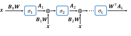
Figure 2: Cascaded gradient network (GradNet-C) defined in (38)-(40), where $\boldsymbol{A}_{\ell}=\mathrm{diag}\left({\boldsymbol{\alpha}_{\ell}}\right)$ and $\boldsymbol{B}_{\ell}=\mathrm{diag}\left({\boldsymbol{\beta}_{\ell}}\right)$.

We propose a cascaded gradient network (GradNet-C), illustrated in Fig. 2 and defined by the layerwise equations

$$\small\boldsymbol{z}_{0} =\boldsymbol{\beta}_{0}\odot\boldsymbol{W}\boldsymbol{x}+\boldsymbol{b}_{0}$$ (38)

$$\boldsymbol{z}_{\ell} =\boldsymbol{\beta}_{\ell}\odot\boldsymbol{W}\boldsymbol{x}+\boldsymbol{\alpha}_{\ell}\odot\sigma_{\ell}(\boldsymbol{z}_{\ell-1})+\boldsymbol{b}_{\ell}$$ (39)

$$\texttt{GradNet-C}(\boldsymbol{x}) =\boldsymbol{W}^{\top}\left[\boldsymbol{\alpha}_{L}\odot\sigma_{L}\left(\boldsymbol{z}_{L-1}\right)\right]+\boldsymbol{b}_{L}$$ (40)

where $\boldsymbol{z}_{\ell},\boldsymbol{b}_{\ell}$, and $\sigma_{\ell}$ respectively denote the output, bias, and activation function at the $\ell$th layer of the network. The weight matrix $\boldsymbol{W}$ is shared across all layers whereas the intermediate scaling weight vectors $\boldsymbol{\alpha}_{\ell},\boldsymbol{\beta}_{\ell}$ are unique to each layer.

Theorem 11 (GradNet-C conditions).

The GradNet-C in (38)-(40) is a GradNet if the $\sigma_{\ell}$ are differentiable elementwise activations.

Proof.

Let $\boldsymbol{A}_{\ell}=\mathrm{diag}\left({\boldsymbol{\alpha}_{\ell}}\right),\boldsymbol{B}_{\ell}=\mathrm{diag}\left({\boldsymbol{\beta}_{\ell}}\right)$. The Jacobian of $\texttt{GradNet-C}(\boldsymbol{x})$ with respect to $\boldsymbol{x}$ is:

$$\boldsymbol{J}_{\texttt{GradNet-C}}(\boldsymbol{x}) =\boldsymbol{W}^{\top}\boldsymbol{D}\boldsymbol{W}$$ (41)

$$\boldsymbol{D} =\sum_{\ell=1}^{L}\left(\prod_{i=0}^{L-\ell}\boldsymbol{A}_{L-i}\boldsymbol{J}_{\sigma_{L-i}}\left(\boldsymbol{z}_{L-i-1}\right)\right)\boldsymbol{B}_{\ell-1}$$ (42)

The activation Jacobians $\boldsymbol{J}_{\sigma_{\ell}}$ are diagonal matrices since each $\sigma_{\ell}$ operates elementwise on the input. Therefore $\boldsymbol{D}$ is a diagonal matrix and $\boldsymbol{J}_{\texttt{GradNet-C}}$ is symmetric. ∎

The activation $\sigma_{\ell}$ in Thm. 11 can be a fixed function applied elementwise, e.g., tanh, softplus, and sigmoid, or a learnable function that operates on individual elements of the input vector. Thus, the proposed approach also permits scalar-valued neural network activation functions as described in Thm. 6. The proposed cascaded networks also remain GradNets if all $\boldsymbol{\beta}_{\ell}$ are 0. However, [36, 37] show that skip connections accelerate training as they address the vanishing gradient problem in deep networks and smoothen the loss landscape.

We now introduce the monotone GradNet-C:

Corollary 11.1 (mGradNet-C conditions).

The GradNet-C in (38)-(40) is an mGradNet, and referred to as mGradNet-C, if, at each layer, the scaling weights $\boldsymbol{\alpha}_{\ell},\boldsymbol{\beta}_{\ell}$ are nonnegative and the $\sigma_{\ell}$ are differentiable, monotonically-increasing elementwise activation functions.

Proof.

Consider $\boldsymbol{J}_{\texttt{GradNet-C}}$ from (41)-(42). By the assumptions in the theorem, for all $\ell$, $\boldsymbol{A}_{\ell},\boldsymbol{B}_{\ell}$ are nonnegative diagonal matrices and the activation Jacobians $\boldsymbol{J}_{\sigma_{\ell}}$ are also nonnegative diagonal matrices. Thus, $\boldsymbol{D}$ is everywhere PSD and it follows that $\boldsymbol{J}_{\texttt{GradNet-C}}$ is everywhere PSD. ∎

The condition in Cor. 11.1 states that the activations $\sigma_{\ell}$ of an mGradNet-C should be monotonically increasing. This condition is not restrictive since most popular elementwise activation functions, e.g., tanh, softplus, and sigmoid, satisfy this requirement and furthermore enables the use of learned, elementwise mGradNet activations as discussed in Thm. 8. While the requirement that the intermediate elementwise scaling weights of mGradNet-C at each layer are nonnegative vectors is more restrictive, it is easy to parameterize in practice. Moreover, we empirically observe in Sec. 7 that imposing nonnegativity constraints on the intermediate weight vectors does not impair optimization or final performance.

6.2 Modular (Monotone) Gradient Networks (GradNet-M, mGradNet-M)

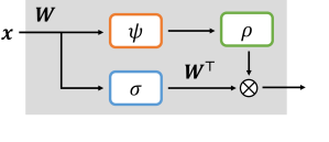
Figure 3: Single module of the modular gradient network (GradNet-M) defined in (43)-(44).

In this section, we describe modular gradient networks (GradNet-M) and their monotone counterparts (mGradNet-M), both of which achieve wider modular architectures by respectively using GradNets and mGradNets, with different weight matrices, as building blocks. GradNet-Ms leverage the facts that a linear combinations of GradNets and a composition of a GradNet with a scalar-valued, differentiable function both yield GradNets, as described respectively in Cor. 2.1 and Thm. 9. We first provide the defining equations for the GradNet-M, after which we give conditions under which the network is a GradNet and an mGradNet.

The GradNet-M is defined by the following equations and generalizes the architecture we previously proposed in [29]:

$$\boldsymbol{z}_{m} =\boldsymbol{W}_{m}\boldsymbol{x}+\boldsymbol{b}_{m}$$ (43)

$$\texttt{GradNet-M}(\boldsymbol{x}) =\boldsymbol{a}+\sum_{m=1}^{M}\rho_{m}(\phi_{m}\left(\boldsymbol{z}_{m}\right))\boldsymbol{W}_{m}^{\top}\sigma_{m}\left(\boldsymbol{z}_{m}\right)$$ (44)

where $\boldsymbol{a}$ denotes a learnable bias and $M$ denotes the number of modules – a hyperparameter tunable based on the application. $\sigma_{m},\boldsymbol{W}_{m}$ and $\boldsymbol{b}_{m}$ respectively denote the activation function, weight matrix, and bias corresponding to the $m^{th}$ module. The block diagram corresponding to a single module output is shown in Fig. 3. The $\phi_{m}$ are vector-to-scalar functions and $\rho_{m}$ are scalar-to-scalar functions. We first provide conditions for $\phi_{m},\rho_{m},$ and $\sigma_{m}$ under which the GradNet-M is a GradNet.

Theorem 12 (GradNet-M conditions).

If $\rho_{m},\phi_{m},\sigma_{m}$ are all differentiable and $\sigma_{m}=\nabla\phi_{m}$, the GradNet-M in (43)-(44) is a GradNet.

Proof.

Consider the $m^{th}$ module $\rho_{m}(\phi_{m}(\boldsymbol{z}_{m}))\boldsymbol{W}_{m}^{\top}\sigma_{m}(\boldsymbol{z}_{m})$. The Jacobian of the $m^{th}$ module with respect to $\boldsymbol{x}$ is

$$\boldsymbol{J}_{m}(\boldsymbol{x}) =\rho_{m}^{\prime}(\phi_{m}(\boldsymbol{z}_{m}))(\boldsymbol{W}_{m}^{\top}\sigma_{m}(\boldsymbol{z}_{m}))(\boldsymbol{W}_{m}^{\top}\sigma_{m}(\boldsymbol{z}_{m}))^{\top}$$

$$\qquad\quad+\rho_{m}(\phi_{m}(\boldsymbol{z}_{m}))\boldsymbol{W}^{\top}_{m}\boldsymbol{J}_{\sigma_{m}}(\boldsymbol{z}_{m})\boldsymbol{W}_{m}$$ (45)

The first term on the RHS is a Gram matrix scaled by $\rho^{\prime}_{m}(\phi_{m}(\boldsymbol{z}_{m}))$, and hence symmetric. The second term on the RHS is symmetric by Thm. 1 since $\boldsymbol{J}^{\top}_{\sigma_{m}}=\boldsymbol{H}_{\phi_{m}}$. Thus, each module is a GradNet and the result holds by Cor. 2.1. ∎

Next, we introduce the monotone GradNet-M:

Corollary 12.1 (mGradNet-M conditions).

The GradNet-M defined by (43)-(44) is an mGradNet, and referred to as mGradNet-M, if, for each module,

1. $\phi_{m}:\mathbb{R}^{d}\to I_{m}\subseteq\mathbb{R}$ is convex, twice differentiable

2. $\rho_{m}:I_{m}\to\mathbb{R}_{\geq 0}$ is differentiable and monotone

3. $\sigma_{m}=\nabla\phi_{m}$

Proof.

The Jacobian of the $m^{th}$ module is given by (6.2). Convexity of $\phi_{m}$ implies $J_{\sigma_{m}}$ is everywhere PSD. Since $\rho_{m}$ is nonnegative-valued, the second term on the RHS of (6.2) is PSD. Monotonicity of $\rho_{m}$ implies that $\rho_{m}^{\prime}$ is everywhere nonnegative, making the first term of (6.2) also PSD. Hence, each module is an mGradNet and the result holds by Cor. 3.1. ∎

While it may appear that the conditions on $\rho_{m},\phi_{m},$ and $\sigma_{m}$ in Cor. 12.1 are restrictive, there are several suitable choices. For example, $\phi_{m}(\boldsymbol{x})=\mathrm{LSE}(\boldsymbol{x})$, $\sigma_{m}(\boldsymbol{x})=\mathrm{softmax}(\boldsymbol{x})$ and $\rho_{m}$ can be any differentiable, monotone nonnegative function on $\mathbb{R}$ such as softplus. As another example, one can take $\sigma_{m}$ to be the elementwise $\mathrm{sigmoid}$ activation function with $\phi_{m}(\boldsymbol{x})=\sum_{i}\mathrm{softplus}(x_{i})$ and $\rho(x)=\alpha x+\beta,\text{ where }\alpha>0$.

7 Experiments

We examine the proficiency of our networks in learning gradients of predefined scalar functions over the unit square.

7.1 Convex Field

We start with the benchmark in [21]:

$$F(x_{1},x_{2})=x_{1}^{4}+\frac{x_{1}^{2}}{2}+\frac{x_{1}x_{2}}{2}+\frac{3x_{2}^{2}}{2}-\frac{x_{2}^{3}}{3}$$ (46)

which is convex on the unit square $x_{1},x_{2}\in[0,1]$. The gradient of the function with respect to the input $\boldsymbol{x}=\begin{bmatrix}x_{1}&x_{2}\end{bmatrix}^{\top}$ is monotone on the unit square and given by

$$\nabla F(x_{1},x_{2})=\begin{bmatrix}4x_{1}^{3}+\frac{1}{2}x_{2}+x_{1}\\ 3x_{2}-x_{2}^{2}+\frac{1}{2}x_{2}\end{bmatrix}$$ (47)

Fig. 4 shows a contour plot of $F$ and a quiver plot of $\nabla F(\boldsymbol{x})$.

We compare the performance of the proposed mGradNet-C and mGradNet-M, respectively defined in (38)-(40) and (43)-(44), with the Input Convex Neural Network (ICNN) [22], Input Convex Gradient Network (ICGN) [21], and Convex Ridge Regularizer (CRR) [11]. The mGradNet-M consists of 4 modules with a hidden dimension of 7, $\rho(x)=1$, and $\sigma(\boldsymbol{x})$ as the softmax function. The outputs of the modules are conically combined via learnable, nonnegative parameters such that the entire network remains monotone in $\boldsymbol{x}$. The mGradNet-C has $L=3$ hidden layers, each with a hidden dimension of 7, elementwise tanh activation, and intermediate nonnegative weight vectors $\boldsymbol{\alpha}_{\ell},\boldsymbol{\beta}_{\ell}$. We use a 2 hidden layer ICNN with hidden dimension 7 and softplus activations, and a zero hidden layer ICGN with hidden dimension 32 and sigmoid activation. The CRR architecture has a hidden dimension of 10 and each learnable spline activation has 7 knots.

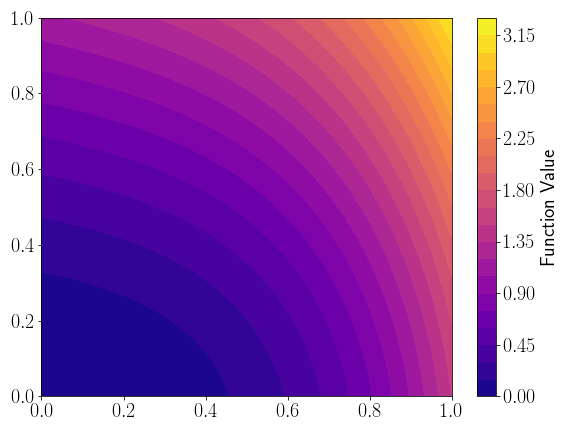
(a) Contour plot of $F(\boldsymbol{x})$

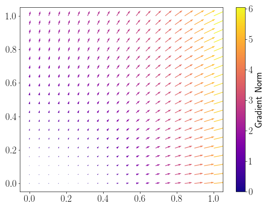
(b) Quiver plot of $\nabla_{\boldsymbol{x}}F(\boldsymbol{x})$

Figure 4: $F(\boldsymbol{x})$ and its corresponding gradient on the unit square.

We sample 100,000 points uniformly at random on the unit square for training and separately sample 10,000 points for validation. Each network, except for the ICNN, takes $\boldsymbol{x}$ as input and is trained to directly output $\nabla F(\boldsymbol{x})$ in (47). The gradient of the ICNN, with respect to $\boldsymbol{x}$, is trained to match $\nabla F(\boldsymbol{x})$. All networks are trained using mean squared error loss for 200 epochs with the Adam optimizer, constant learning rate of 0.005, and minibatch size of 1000. To compare the relative expressiveness of the networks, they have approximately the same number of parameters. The trained models are tested using 10,000 uniformly spaced points within the unit square. We repeat the training and testing procedure for 5 trials.

Table 1: RMSE from estimating monotone gradient $\nabla F(\boldsymbol{x})$ in (47) over the unit square (5 trials). *Our methods.

		RMSE (dB)
Model	Parameters	Mean	Std
ICNN [22]	109	-17.13	2.53
ICGN [21]	96	-10.61	0.80
CRR [11]	102	-15.70	2.04
mGradNet-C*	100	-24.08	0.44
mGradNet-M*	94	-23.57	2.61

Table 1 reports the average root mean squared error (RMSE) across all trials in log scale. The proposed mGradNet-M and mGradNet-C exhibit significantly lower error rates than that of the ICNN, ICGN, and CRR. The mGradNet-M and mGradNet-C respectively achieve roughly 6 and 7 dB lower RMSE than the ICNN, the best among the baselines. Fig. 5 illustrates the $\ell_{2}$ norm difference between the gradient predicted by each model and the true gradient of $\nabla F(\boldsymbol{x})$ at each point in the unit square.

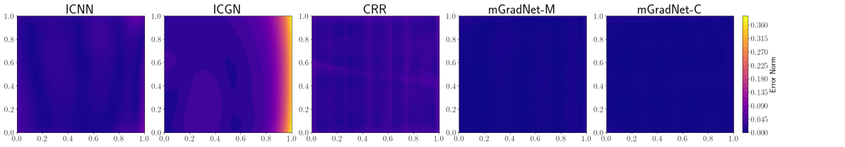
Figure 5: $\ell_{2}$ norm of error between predicted and true gradient $\nabla F$ in (47) at each point $\boldsymbol{x}=(x_{1},x_{2})$ in the unit square.

The error visualizations of the proposed mGradNet-M and mGradNet-C exhibit fewer artifacts than the error plots of the ICNN, ICGN and CRR, which reflects more accurate learning across the unit square.

7.2 Nonconvex Field

Next, we study the efficacy of our networks in learning gradients of nonconvex functions.

Our experiment uses the gradient of the function

$$G(\boldsymbol{x}) =\frac{1}{4}\sin(2\pi x_{1})\cos(\pi x_{2})+\frac{x_{1}x_{2}}{2}-\frac{x_{2}^{2}}{2}$$ (48)

The function exhibits several stationary points within the unit square, as illustrated in Fig. 6(a). As before, we consider learning $\nabla G$, which is illustrated in Fig. 6(b) and given by

$$\nabla G(\boldsymbol{x}) =\begin{bmatrix}\frac{\pi}{2}\cos(2\pi x_{1})\cos(\pi x_{2})+\frac{x_{2}}{2}\\ -\frac{\pi}{4}\sin(2\pi x_{1})\sin(\pi x_{2})+\frac{x_{1}}{2}-x_{2}\end{bmatrix}$$ (49)

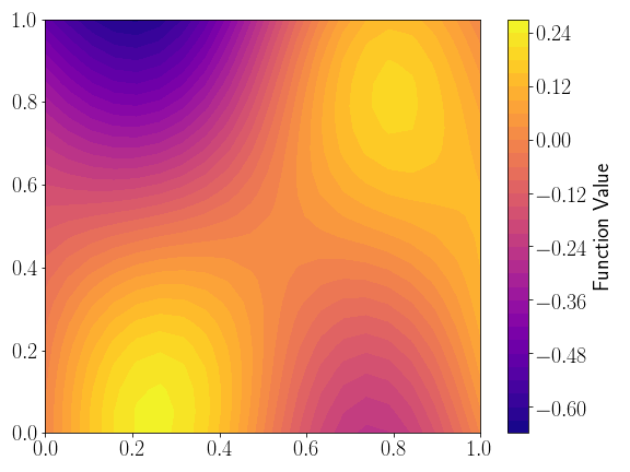
(a) Contour plot of $G(\boldsymbol{x})$

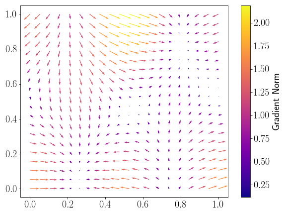
(b) Quiver plot of $\nabla G(\boldsymbol{x})$

Figure 6: $G(\boldsymbol{x})$ and its corresponding gradient on the unit square.

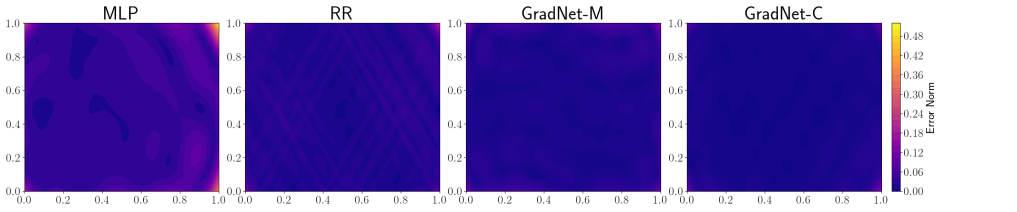
Figure 7: $\ell_{2}$ norm of error between predicted and true gradient $\nabla G$ in (49) at each point $\boldsymbol{x}=(x_{1},x_{2})$ in the unit square.

We evaluate the performance of the proposed modular gradient network (GradNet-M) and cascaded gradient network (GradNet-C) for learning $\nabla G(\boldsymbol{x})$ on the unit square and compare the performance to that of a multilayer perceptron (MLP) and the ridge regularizer (RR) network proposed in [11]. The ridge regularization function from [11] has the same architecture as the CRR used in the convex gradient field experiment, however the spline activation functions are no longer constrained to be monotonically increasing. The input to the RR, GradNet-M, and GradNet-C is again the point $\boldsymbol{x}$ and the networks are trained to directly output $\nabla G(\boldsymbol{x})$. The input to the MLP is also $\boldsymbol{x}$ and the gradient of the MLP, with respect to $\boldsymbol{x}$, is trained to be $\nabla G(\boldsymbol{x})$. GradNet-M has the same architecture as the mGradNet-M used in the prior experiment, however the module outputs are linearly combined using learnable parameters that can be negative. The GradNet-C also has the same architecture as the mGradNet-C from the prior experiment except the intermediate weight vectors $\boldsymbol{\alpha},\boldsymbol{\beta}$ are no longer constrained to be nonnegative. The nonconvex gradient field is performed using the same number of data samples and optimization hyperparameters as described for the convex field experiment.

Table 2: RMSE from estimating gradient $\nabla G(\boldsymbol{x})$ in (49) over the unit square ($G$ nonconvex; 5 trials). *Our methods.

		RMSE (dB)
Model	Parameters	Mean	Std
MLP	102	-12.83	1.04
RR [11]	102	-16.23	1.83
mGradNet-C*	100	-18.99	2.03
mGradNet-M*	94	-17.00	1.90

Table 2 reports the average RMSE across 5 trials in log scale. As in the convex field experiment, the cascaded architecture performs the best among the considered model architectures. The proposed cascaded architecture, GradNet-C, achieves the best performance – which is nearly 3 dB better than the baseline ridge regularizer proposed in [11]. The $\ell_{2}$ error plots in Fig. 7 show that GradNet-C learns the gradient nearly everywhere in the unit square, whereas other methods struggle to learn the gradient near the corners of the square.

8 Conclusion

This paper presented gradient networks, novel classes of neural networks for directly parameterizing and learning gradients of functions. We first introduced gradient networks that are guaranteed to be gradients of scalar-valued functions. We subsequently demonstrated methods to convert gradient networks into monotone gradient networks that specifically correspond to the gradients of convex functions. In addition, we proposed a general framework for designing (monotone) gradient networks and established their universal approximation capabilities. Our experimental results on gradient field learning problems not only highlight the theoretical underpinnings of GradNets and mGradNets, but also demonstrate their utility in practical applications.

References

- [1] A. Krizhevsky, I. Sutskever, and G. E. Hinton, “Imagenet classification with deep convolutional neural networks,” Advances in Neural Information Processing Systems, vol. 25, 2012.
- [2] A. Vaswani, N. Shazeer, N. Parmar, J. Uszkoreit, L. Jones, A. N. Gomez, Ł. Kaiser, and I. Polosukhin, “Attention is all you need,” Advances in Neural Information Processing Systems, vol. 30, 2017.
- [3] V. Mnih, K. Kavukcuoglu, D. Silver, A. A. Rusu, J. Veness, M. G. Bellemare, A. Graves, M. Riedmiller, A. K. Fidjeland, G. Ostrovski et al., “Human-level control through deep reinforcement learning,” Nature, vol. 518, no. 7540, pp. 529–533, 2015.
- [4] A. Hyvärinen and P. Dayan, “Estimation of non-normalized statistical models by score matching.” Journal of Machine Learning Research, vol. 6, no. 4, pp. 695–709, 2005.
- [5] Y. Song and S. Ermon, “Generative modeling by estimating gradients of the data distribution,” Advances in Neural Information Processing Systems, vol. 32, 2019.
- [6] R. Cai, G. Yang, H. Averbuch-Elor, Z. Hao, S. Belongie, N. Snavely, and B. Hariharan, “Learning gradient fields for shape generation,” in Computer Vision–ECCV 2020: 16th European Conference, Glasgow, UK, August 23–28, 2020, Proceedings, Part III 16. Springer, 2020, pp. 364–381.
- [7] C. Shi, S. Luo, M. Xu, and J. Tang, “Learning gradient fields for molecular conformation generation,” in International Conference on Machine Learning. PMLR, 2021, pp. 9558–9568.
- [8] Y. Brenier, “Polar factorization and monotone rearrangement of vector-valued functions,” Communications on Pure and Applied Mathematics, vol. 44, no. 4, pp. 375–417, 1991.
- [9] F. Santambrogio, “Optimal transport for applied mathematicians,” Birkäuser, NY, vol. 55, no. 58-63, p. 94, 2015.
- [10] C.-W. Huang, R. T. Q. Chen, C. Tsirigotis, and A. Courville, “Convex potential flows: Universal probability distributions with optimal transport and convex optimization,” in International Conference on Learning Representations, 2021. [Online]. Available: https://openreview.net/forum?id=te7PVH1sPxJ
- [11] A. Goujon, S. Neumayer, P. Bohra, S. Ducotterd, and M. Unser, “A neural-network-based convex regularizer for inverse problems,” IEEE Transactions on Computational Imaging, vol. 9, pp. 781–795, 2023.
- [12] R. Cohen, Y. Blau, D. Freedman, and E. Rivlin, “It has potential: Gradient-driven denoisers for convergent solutions to inverse problems,” Advances in Neural Information Processing Systems, vol. 34, pp. 18 152–18 164, 2021.
- [13] R. Fermanian, M. Le Pendu, and C. Guillemot, “PnP-ReG: Learned regularizing gradient for plug-and-play gradient descent,” SIAM Journal on Imaging Sciences, vol. 16, no. 2, pp. 585–613, 2023.
- [14] Y. Song and S. Ermon, “Improved techniques for training score-based generative models,” Advances in Neural Information Processing Systems, vol. 33, pp. 12 438–12 448, 2020.
- [15] M. Andrychowicz, M. Denil, S. Gomez, M. W. Hoffman, D. Pfau, T. Schaul, B. Shillingford, and N. De Freitas, “Learning to learn by gradient descent by gradient descent,” Advances in Neural Information Processing Systems, vol. 29, 2016.
- [16] W. Rudin, Principles of mathematical analysis. McGraw-hill New York, 1964, vol. 3.
- [17] W. M. Czarnecki, S. Osindero, M. Jaderberg, G. Swirszcz, and R. Pascanu, “Sobolev training for neural networks,” Advances in Neural Information Processing Systems, vol. 30, 2017.
- [18] D. B. Lindell, J. N. P. Martel, and G. Wetzstein, “AutoInt: Automatic integration for fast neural volume rendering,” in Proceedings of the IEEE/CVF Conference on Computer Vision and Pattern Recognition (CVPR), June 2021, pp. 14 556–14 565.
- [19] S. Saremi, “On approximating with neural networks,” arXiv preprint arXiv:1910.12744, 2019.
- [20] L. Metz, C. D. Freeman, S. S. Schoenholz, and T. Kachman, “Gradients are not all you need,” arXiv preprint arXiv:2111.05803, 2021.
- [21] J. Richter-Powell, J. Lorraine, and B. Amos, “Input convex gradient networks,” arXiv preprint arXiv:2111.12187, 2021.
- [22] B. Amos, L. Xu, and J. Z. Kolter, “Input convex neural networks,” in International Conference on Machine Learning. PMLR, 2017, pp. 146–155.
- [23] Y. Chen, Y. Shi, and B. Zhang, “Optimal control via neural networks: A convex approach,” International Conference on Learning Representations, 2018.
- [24] A. Makkuva, A. Taghvaei, S. Oh, and J. Lee, “Optimal transport mapping via input convex neural networks,” in International Conference on Machine Learning. PMLR, 2020, pp. 6672–6681.
- [25] A. Korotin, L. Li, A. Genevay, J. M. Solomon, A. Filippov, and E. Burnaev, “Do neural optimal transport solvers work? a continuous wasserstein-2 benchmark,” Advances in Neural Information Processing Systems, vol. 34, pp. 14 593–14 605, 2021.
- [26] P. J. Davis and P. Rabinowitz, Methods of Numerical Integration. Courier Corporation, 2007.
- [27] T. Tao, Analysis II. Springer, 2016.
- [28] J. M. Lee, Smooth Manifolds. Springer, 2012.
- [29] S. Chaudhari, S. Pranav, and J. M. Moura, “Learning gradients of convex functions with monotone gradient networks,” in ICASSP 2023 - 2023 IEEE International Conference on Acoustics, Speech and Signal Processing (ICASSP), 2023, pp. 1–5.
- [30] R. T. Rockafellar and R. J.-B. Wets, Variational Analysis. Springer Science & Business Media, 2009, vol. 317.
- [31] S. Boyd, S. P. Boyd, and L. Vandenberghe, Convex Optimization. Cambridge University Press, 2004.
- [32] R. T. Rockafellar, Convex Analysis. Princeton University Press, 1970, vol. 18.
- [33] A. H. Smith and W. A. Albrecht, Fundamental Concepts of Analysis. Prentice-Hall, 1966.
- [34] A. L. Yuille and A. Rangarajan, “The concave-convex procedure (CCCP),” Advances in Neural Information Processing Systems, vol. 14, 2001.
- [35] G. Cybenko, “Approximation by superpositions of a sigmoidal function,” Mathematics of Control, Signals and Systems, vol. 2, no. 4, pp. 303–314, 1989.
- [36] K. He, X. Zhang, S. Ren, and J. Sun, “Deep residual learning for image recognition,” in Proceedings of the IEEE Conference on Computer Vision and Pattern Recognition, 2016, pp. 770–778.
- [37] H. Li, Z. Xu, G. Taylor, C. Studer, and T. Goldstein, “Visualizing the loss landscape of neural nets,” Advances in Neural Information Processing Systems, vol. 31, 2018.