Recovering the gas properties of protoplanetary disks through parametric visibility modeling: MHO 6

Abstract

Context. The composition and distribution of the gas in a protoplanetary disk plays a key role in shaping the outcome of the planet formation process. Observationally, the recovery of information such as the emission height and brightness temperature from interferometric data is often limited by the imaging processes.

Aims. To overcome the limitations of image-reconstruction when analyzing gas emission from interferometric observations, we have introduced a parametric model to fit the main observable properties of the gaseous disk component in the visibility plane. This approach is also known as parametric visibility modeling.

Methods. We applied our parametric visibility modeling to the gas brightness distribution of the molecular line emission from ¹²CO J=3-2 and ¹³CO J=3-2 in the disk around MHO 6, a very-low-mass star in the Taurus star-forming Region. To improve the flux fidelity of our parametric models, we combined models with different pixel resolution before the computation of their visibilities, referred to as “nesting images.”

Results. When we apply our parametric visibility modeling to MHO 6, with independent fits to the emission from its CO isopotologues, the models return the same consistent results for the stellar mass, disk geometry, and central velocity. The surface height and brightness temperature distribution are also recovered. When compared to other disks, MHO 6 surface height is among the most elevated surfaces, consistent with the predictions for disks around very-low-mass stars.

Conclusions. This work demonstrates the feasibility of running rapidly iterable parametric visibility models in moderate resolution and sensitivity interferometric observations. More importantly, this methodology opens the analysis of disk’s gas morphology to observations where image-based techniques are unable to robustly operate, as in the case of the compact disk around MHO 6.

1 Introduction

The gas emission of protoplanetary disks is a key observational tracer of the temperature distribution (e.g., Schwarz et al. 2016; Zhang et al. 2021), kinematics (e.g., Teague 2019; Wölfer et al. 2023), morphology of the emitting region (e.g., Pinte et al. 2018; Law et al. 2021b; Paneque-Carreño et al. 2023), and chemical properties (e.g., Öberg et al. 2021). All of these properties play a key role in shaping the architecture and composition of forming planets. The majority of these studies have only become possible through the superb sensitivity and angular resolution of interferometers such as the Atacama Large (sub-)Millimeter Array (ALMA). Interferometers sample the Fourier transform of the observed source, also known as the “visibilities” (for a more detailed explanation, we refer to Czekala et al. 2021, and references therein), and images of the brightness distribution need to be reconstructed from the visibilities with algorithms such as CLEAN (Högbom 1974; Clark 1980; Briggs 1995) or maximum entropy and likelihood methods (e.g., Ponsonby 1973; Ables 1974; Cornwell & Evans 1985; Narayan & Nityananda 1986; Casassus et al. 2006; Cárcamo et al. 2018). Even though the visibility coverage of ALMA is dense enough to recover high fidelity reconstructed images of its observations, any analysis performed on those images will be dependent on the specific imaging method chosen, as different images can deviate with regard to their features (see Zawadzki et al. 2023).

In the case of low signal-to-noise ratio (S/N) observations, information recovery from interferometric data can be maximized when assuming that the brightness distribution follows a coherent morphology. This is a common assumption for protoplanetary disks, which have a dominant axisymmetric structure (e.g., Andrews et al. 2018; Long et al. 2018; Cieza et al. 2021). In the dust continuum emission, applying priors on the morphology of disks allows for parametric (e.g., Tazzari et al. 2017) and non-parametric (e.g., Jennings et al. 2020) models to successfully recover very small-scale structures (e.g., Kurtovic et al. 2022; Jennings et al. 2022), to search for faint emitting sources (e.g., Andrews et al. 2021), and to characterize disk sizes and brightness distribution (e.g., Hendler et al. 2020). The visibility modeling of the gas emission, however, has the additional challenge of generating velocity-dependent models to follow the disk’s rotation, which considerably increases the difficulty of implementing prior emission morphologies compared to the dust visibility modeling. Nevertheless, visibility-based approaches to analyzing the gas emission of protoplanetary disks have been applied when recovering the turbulence level of disks (e.g., Flaherty et al. 2015, 2020) and the dynamical mass of stellar hosts (Czekala et al. 2015; Pegues et al. 2021; Long et al. 2021), as well as in match-filtering faint emission (Loomis et al. 2018).

In this work, we explore the advantages and limitations of describing the properties of the gas surface-emitting layer with a parametric visibility-based modeling. Our aim is to extend the tools that are widely used to analyze dust continuum emission to the gas emission observations. We analyze the source MHO 6, an M5.0 star a mass of $M_{\star}\sim 0.2\,M_{\odot}$ (Kurtovic et al. 2021; Pegues et al. 2021), located in the Taurus star-forming region at 154 pc (Gaia DR3, Gaia Collaboration et al. 2021). MHO 6 was chosen as it is spatially resolved in dust continuum and ¹²CO J=3-2 emission when observed with 15 au resolution. Also, it is one of the few disks around a very low mass star (VLMS) with a large gap at millimeter wavelengths (Pinilla 2022), which could have been produced by planet-disk interaction (Kurtovic et al. 2021). In the 0.9 mm continuum, MHO 6 shows a single ring peaking at 11 au; while in the gas emission, the disk extends for approximately 200 au in radius. Unlike several other VLMS disks in the Taurus Region, the CO isotopologue emission in the MHO 6 disk is not completely absorbed by the cloud in the low-velocity channels (e.g., Kurtovic et al. 2021; Hashimoto et al. 2021). This allows us to detect the disk in blueshifted and redshifted molecular line emission, with some absorption detected close to the systemic velocity of MHO 6. Due to its moderate brightness and relatively small angular extent, MHO 6 is not an ideal source to be studied in the image plane, as it would need to be targeted with very extended baselines for long exposure times. For these reasons, we chose to describe the disk morphology directly in the visibilities.

In Sect. 2, we summarize the observations analyzed in this work. In Sect. 3 we describe the visibility fitting process, and we introduce our solution for generating intensity models of the inner disk emission. We present the results of our modeling in Sect. 4, and we further discuss the benefits and limitations of our visibility approach in Sect. 5. Finally, we present our conclusions in Sect. 6.

2 Observations

This work includes 0.87 mm observations of the disk around MHO 6. The dataset was obtained by ALMA in Band 7, as part of the project 2018.1.00310.S (PI: P. Pinilla). The self-calibration and data preparation process was already published in Kurtovic et al. (2021). As a summary, our observations include two spectral windows covering dust continuum emission: one spectral window covering the molecular line ¹²CO J=3-2 transition (from now on referred to as ¹²CO) and one spectral window covering the molecular line ¹³CO J=3-2 transition (from now on referred to as ¹³CO). With CASA 5.6.2 (McMullin et al. 2007), we averaged the continuum-subtracted measurement sets into $30$ s bins to reduce data volume. We applied the task cvel2 to the self-calibrated and time-binned ¹²CO, redefining the channels to start from -3.5 km s^-1, with 0.5 km s^-1 of channel width to increase the S/N of the emission, using 32 channels in total. This range covers the channels where emission was detected, along with a few channels with undetected emission on each side of the line. Compared to the native frequency resolution of the observation, we increased the channel width from 244.1 kHz to 576.7 kHz. For the ¹³CO, we started from -3.5 km s^-1 with 0.9 km s^-1 of channel width, using 19 channels in total to cover a similar velocity range as the ¹²CO. The visibility table of each channel was extracted and converted to wavelength units using each channel central frequency.

For visual reference, we generated image cubes of each line with the CASA task tclean, with a robust parameter of 0.5 to obtain a good balance between the sensitivity and the angular resolution. No visibility tapering was applied. The beam size for the ¹²CO cube is $110\times 80$ mas with a position angle of $31.5\,$deg. The ¹³CO cube has a resolution of $124\times 89$ mas with a position angle of $34.6\,$deg. Thus, the spatial resolution of each image cube is about $16\times 12$ au and $18\times 13$ au for ¹²CO and ¹³CO, respectively. Additional image cubes from synthetic models or residuals were reconstructed with the same tclean setup, and they share the observations angular resolution.

3 Methodology: Parametric visibility modeling

We analyze the ¹²CO and ¹³CO emission of MHO 6 directly in the visibility plane. To do so, we followed a similar approach as that applied to the continuum visibility modeling presented in Kurtovic et al. (2022). We generated a model image following a parametric description for the intensity distribution, and we used the galario package (Tazzari et al. 2017) to calculate the visibilities of the model. When fitting gas emission, an image has to be generated for each fitted channel, as the brightness distribution is velocity-dependent. Therefore, we generated 32 images to fit the ¹²CO and 19 for the ¹³CO.

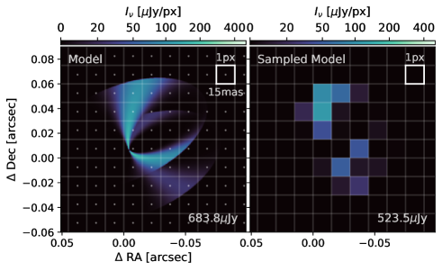
Figure 1: Left panel: Image representative of the parametric model for the inner 10 au intensity distribution of a single velocity channel of MHO 6 (centered at 6 km s^-1). The total flux from the image is shown in the lower right corner. The white lines represent the pixel grid used to sample the intensity distribution, prior to calculating its visibilities. The white dots show the location of the pixels center. Right panel: Sampled model image, where each pixel has the value of the intensity distribution evaluated at the pixel center. Each pixel is 15 mas per side, close to 2 au at the distance of MHO 6. Due to an incomplete intensity sampling, the total flux is underestimated.

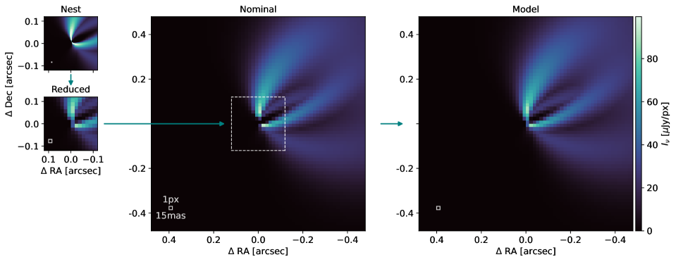
Figure 2: Example of the nesting image process. The nest image is averaged into the reduced image, which then replaces the center of the nominal image to obtain the model image. In this example, the nest image was generated with a nest of level $n=3$. The pixel size is shown with a square in the bottom left corner of each panel.

3.1 Elevation, intensity, and combination of emitting layers

The intensity distribution was calculated over a coordinate system that considers the elevation of the emitting layers. Those coordinates were calculated based on the functions from the python package eddy (Teague 2019), which are organized for image cube generation in the git-hub repository wrinkleology (Teague 2022). Two emitting layers are calculated for each line: front (upper) and back (bottom), one on each side of the midplane. The height of the emission surface $z(r)$ is described with an exponentially tapered power law as a function of the radial distance from the star $r$, as its commonly done in the literature (e.g., Teague 2019; Law et al. 2021b; Izquierdo et al. 2021). As an approximation for both CO isotopologues, we imposed the front and back layer should have the same height ($z_{b}=-z_{f}$) relative to the disk midplane (see Section 5 for a discussion on this decision). The equation describing $z_{f}$ is thus given by:

$$z_{f}(r)\,=\,z^{\prime}_{f0}\cdot\left(\frac{r}{r_{0}}\right)^{\psi}\cdot\exp\left(-\left(\frac{r}{r_{z}}\right)^{\phi}\right)\text{,}$$ (1)

where $z^{\prime}_{f0}$ is the elevation of the emitting layer at a distance $r_{0}$, before being tapered by the exponential part of the function. This function has a degeneracy between the parameters $z^{\prime}_{f0}$ and $r_{0}^{\psi}$, which can be combined into $z_{f0}=z^{\prime}_{f0}/r_{0}^{\psi}$, the equivalent to fixing $r_{0}=1^{\prime\prime}$ for a radial distance given in units of arcseconds (as in Law et al. 2021b). This reduces the number of free parameters describing the elevation of the emitting surface to four: $(z_{f0},\psi,\phi,r_{z})$.

Next, we set the intensity of the front layer $I_{f}(r)$ of each pixel as a function of its central coordinates in the disk-frame. We chose to also describe it with an exponentially tapered power law, following:

$$\centering I_{f}(r)\,=\,I^{\prime}_{f0}\cdot\left(\frac{r}{r_{0}}\right)^{\alpha}\cdot\exp\left(-\left(\frac{r}{r_{I}}\right)^{\beta}\right)\text{.}\@add@centering$$ (2)

During the calculation, the transformation, $I_{f0}=I^{\prime}_{f0}/r_{0}^{\alpha}$, is also applied, with the same assumption over $r_{0}$ as in $z_{f}$. For the back layer, the intensity, $I_{b}$, is also described as in Eq. 2, but with different values for $(I_{f0},\alpha,\beta)$ and sharing $r_{I}$ with $I_{f}$.

To calculate the emission of individual channel maps, the intensity of the emitting layers ($I_{f}$, $I_{b}$) has to be filtered as a function of the projected velocity of each pixel $v_{proj}$. In the current model, the velocity field is approximated to be purely Keplerian, which is only consistent with disks where $M_{\text{disk}}\ll M_{\star}$, and without local perturbations from stellar companions or planets. Additionally, we assumed a Gaussian line-broadening in the velocity, where the linewidth of the emission in each pixel is described as a function of the radii:

$$\centering\delta v(r)\,=\,\delta v^{\prime}_{0}\cdot\left(\frac{r}{r_{0}}\right)^{-q}\text{,}\@add@centering$$ (3)

where $\delta v^{\prime}_{0}$ is the linewidth at the distance $r_{0}$, which we fix to $r_{0}=1^{\prime\prime}$. Then, for a certain channel $k$ with a central velocity $v_{k}$, the contribution of a pixel with projected velocity $v_{proj}$ to the intensity of the front layer emission $I_{f}$ is given by:

$$\centering I_{f,k}\,=\,I_{f}\cdot\exp\left(-\frac{1}{2}\left(\frac{v_{proj}-v_{k}}{\delta v}\right)^{2}\right)\text{,}\@add@centering$$ (4)

where we assumed that $I_{f}$ has been projected onto the sky plane, and is described in the same coordinate system as $v_{proj}$. The same calculation is performed to obtain $I_{b,k}$, which describes the back layer emission. We include an additional parameter to describe a possible cavity in the the $I_{f}$ and $I_{b}$ emission, called $r_{cav}$. This parameters shifts the beginning of the brightness profile by a distance of $r_{cav}$ from the center.

After obtaining the emission of each layer in a specific channel $k$, the next step for generating the model image of the channel is to combine the emission of the front and the back layer into a single image. For simplicity, we assume that the intensity value of each pixel in the model image is the maximum between upper and lower emission surface:

$$\centering I_{k}=\left\{\begin{aligned} I_{f,k}\,\text{,}&\hskip 17.07182pt\text{for }I_{f,k}\geq I_{b,k}\\ I_{b,k}\,\text{,}&\hskip 17.07182pt\text{for }I_{f,k}<I_{b,k}\\ \end{aligned}\right.\text{,}\@add@centering$$ (5)

which is a first approximation for an optically thick front layer over the whole channel velocity width. This assumption is also considered in similar frameworks, such as discminer (Izquierdo et al. 2021) and it has shown to be a good first approach to describe the ¹²CO emission from young circumstellar disks (e.g., Izquierdo et al. 2022). An example of combining layers in a single channel through this method is shown in the left panel of Fig. 1. We also attempted an alternative combination, different from this binary selection between $I_{f,k}$ and $I_{b,k}$, with a smooth transition with a power law weighting. This alternative did not produce significant improvements over the fitting, and its details are described in the Appendix B.

As the CO lines from MHO 6 are affected by surrounding cloud absorption, this contribution needs to be considered in order to fit the flux distribution of each channel. We assume that the absorption decreases the emission of the whole channel by a proportional factor as a function of velocity, which we describe with a Gaussian function ($G_{ext}$). This parametrization of the absorption has three free parameters: the velocity center ($c_{v0}$), the velocity width ($c_{\sigma}$), and the amplitude of the absorption ($c_{a}$), which we fit for both CO isotopologues. No cloud contribution in positive emission was considered in our fitting.

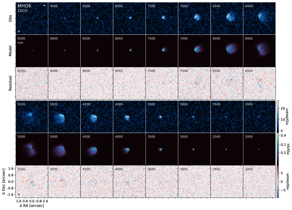
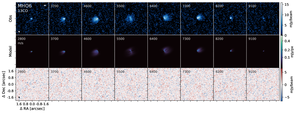
Figure 3: ¹²CO J=3-2 and ¹³CO J=3-2 channel maps. Each row shows the CLEAN image of the observation, the best visibility model, and the image made from the residual visibilities. The scale bar in the upper left panels is 10 au in size, while the beam size is shown in the lower left corner of the first panels. The number in the upper left corner shows the channel velocity relative to the resting frequency of each line, in m s^-1.

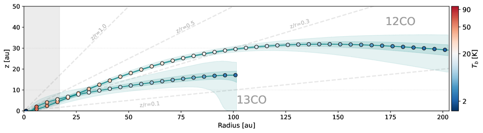
Figure 4: Height of the surface emitting layer for the ¹²CO and ¹³CO of MHO 6. The darker and lighter shaded regions surrounding each profile represent the $1\sigma$ and $3\sigma$ confidence levels, respectively. The grey shaded region on the left shows the spatial extent of one angular resolution element, as measured from the disk center. The distance in the x-y axis is shown in a 1:1 scale.

3.2 Nesting images

The method of visibility fitting is based on matching the visibilities of an observation to those calculated from a given intensity distribution model. Since the model visibilities are calculated numerically, an underlying assumption is that the brightness associated with each pixel is representative of the flux contained inside the region covered by the pixel extent. As an example, let us assume a parametric function that describes $I_{k}$ (the intensity of a channel $k$), represented in the left panel of Fig. 1 with extremely high spatial resolution. In order to numerically calculate the visibilities of this channel, we need to create an image of $I_{k}$ (the “sampled Model”), shown in the right panel of Fig. 1. The pixel size of 15 mas is comparable to the pixel size in high angular resolution observations of gas tracers with ALMA. In the sampled model, the value of each pixel is the value of the function at the center of the pixel; thus, if the pixel size is larger than the scale of spatial variations in the intensity model, the flux contained in each pixel will not be representative of the integrated flux inside such a region. This effect commonly leads to flux underestimation in the inner regions of the disk, as shown with a 10 au disk in Fig. 1, and it can influence the fitting even if the affected region is spatially unresolved. To overcome this problem, the pixel size needs to be small enough to sample each channel intensity distribution. In a single image, such pixel size can be prohibitively small for the inner disk region, forcing the number of pixels contained in an image to be unnecessarily large to properly cover the outer regions of the disk.

We explored a solution to the issue of Fig. 1 by generating two images of the same intensity distribution: The first covers an extended field of view that includes the whole disk emission, while the second is smaller and has a higher pixel resolution to sample the inner disk region. In the following, we refer to the first image as the “nominal”, and the second as the “nest,” as exemplified in Fig. 2. To combine both, we averaged the pixels of the nest image to match the pixel size of the nominal, creating a “reduced” image. Then, the central section of the nominal image is replaced with the reduced image, obtaining a “model” image with the same image size and pixel size as the nominal, but with a higher flux fidelity. We further refer to this process as “nesting” images.

We explored oversampling the pixels of the nominal image in multiples of 4. Thus, an image with no nesting would be the same as oversampling with a factor of $4^{0}$; one level of nesting would mean that every pixel in the nominal image is oversampled with $4^{1}$ pixels; and, more generally, an $n$ level of nesting means that every nominal pixel in the central region is oversampled with $4^{n}$ pixels. An example of the difference between using different levels of nesting, up to level 6, is shown in Fig. 11 in the appendix, where the flux of each pixel in the reduced image is compared to that of an image generated with model with a nesting level of 6. A more detailed exploration of flux conservation with nested images is also given in Section C in the Appendix. For MHO 6, we used a nominal image of 512 px in size, with each pixel being 15 mas. The inner 64 pixels of the nominal image are replaced by a nest image of level $n=2$, which means that it oversamples the nominal pixel with $4^{n=2}$ pixels. The size of the region covered by the nest image is determined empirically, and we discuss this topic further in Sect. 5.4.

3.3 MCMC fitting

We fitted both CO isotopologues independently, with the same parametric functions. Thus, parameters such as the disk geometry ($\Delta$RA, $\Delta$Dec, inc, PA), stellar mass ($M_{\star}$), central disk velocity, and cloud velocity (VLSR, c_v0), are allowed to be different for each line, to test for consistency. We sampled each parameter density distribution with the Markov chain Monte Carlo (MCMC) code emcee (Foreman-Mackey et al. 2013), using eight times the number of walkers with respect to the free parameters. Each parameter has a flat uniform prior over the allowed parameter range, which extends far enough so that the walkers do not interact with it. Each model results are sampled from the last $10^{5}$ steps, after a burning period of at least $10^{5}$ steps.

4 Results

The results of our MCMC fitting are shown in Fig. 3 for a subset ¹²CO and ¹³CO channels around the central velocity. Both CO isotopologues find consistent solutions for the shared parameters, such as the midplane geometry, the stellar mass, $M_{\star}$, and the central velocity, VLSR. The ¹²CO emission constrains $M_{\star}=0.164\pm 0.003$, which is consistent with the ¹³CO modeling result, and also with the literature (Ward-Duong et al. 2018; Kurtovic et al. 2021; Pegues et al. 2021). Furthermore, the models successfully disentangle the regions corresponding to the front and back emitting layers, which allows us to estimate their brightness temperature profiles. The front emitting layer of the ¹²CO emission reaches its maximum height at a radii of about $100$ to $125$ au, close to the $z/r=0.3$ ratio, after which it starts declining towards the midplane, as shown in Fig. 4. Starting from about 20 au, the best model for the ¹³CO emission has a height below that of the ¹²CO. Within the first 20 au, which closely coincides with the spatial resolution of the dataset, the height of the ¹²CO and ¹³CO are consistent within the $1\sigma$ limit. We note that the turnover parameters $\beta_{f}$ and $\phi$ of the ¹³CO emission are very unconstrained, as the turnover distances, $r_{z}$ and $r_{I}$, coincide with the $R_{95\%}$.

Our fitting also recovers the magnitude of cloud transparency as a function of velocity. As expected, the ¹³CO emission is less affected by the cloud absorption, with the lowest transparency being approximately $70\%$ at the central velocity of the disk. On the other hand, the ¹²CO emission has the lowest transparency of $50\%$ at the central velocity channel. By knowing the magnitude of the absorption, we can correct the measured fluxes of each disk, as listed in Table 1. All our analyses of the disk sizes and temperature were carried out with the absorption-corrected models.

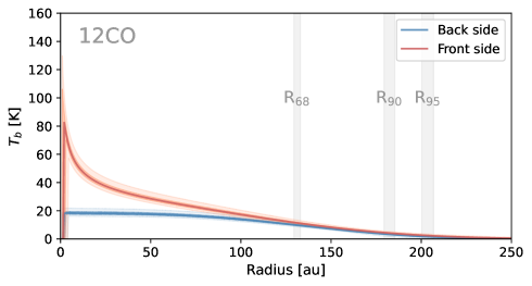
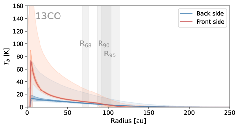
Figure 5: Azimuthally averaged brightness temperature profile for the ¹²CO and ¹³CO emission in the upper and lower panel, respectively. The darker and lighter shaded regions represent the $1\sigma$ and $3\sigma$ uncertainty of the brightness temperature, respectively. The solid line shows the best model. The vertical bands in grey show the $3\sigma$ radii region that includes the 68%, 90% and 95% of the emission.

Our channel-by-channel model describes the ¹³CO emission down to the sensitivity level of the observation, leaving no significant residuals in the reconstructed image. In the ¹²CO emission, however, structured low-contrast non-axisymmetric residuals are detected around the central velocity channels, which we further discuss in Sect. 5. We calculated the brightness temperature of each model by converting the emission from intensity units in Jy px^-1 to temperature in Kelvin. This was done under the Rayleigh-Jeans approximation for black body emission in the low frequency regime, assuming the emission is entirely optically thick. Thus, the azimuthal profile of the brightness temperature is directly recovered from our fitting to both CO isotopologues, as shown in Fig. 5.

The size of the disk is measured by constraining the radii enclosing $68\%$, $90\%$, and $95\%$ of the total flux as measured from the front layer emission surface. Those values are listed in Table 1 for both lines and also shown to their $1\sigma$ confidence in Fig. 5. Despite using a different definition when measuring the disk size, we found values that are consistent with those measured from integrating the moment 0 emission with an elliptical aperture in Kurtovic et al. (2021). Therefore, we confirm the gas to dust size ratio of 3.9 when comparing the 0.87 mm emission to the ¹²CO J=3-2 emission. It is not uncommon to observe such a high ratio among young disks (Long et al. 2022) and it suggests that radial drift has influenced the disk evolution (Trapman et al. 2019). Interestingly, both the front and back emission layer converge to the same brightness temperature at the $R_{68\%}$ size of the front layer in both CO isotopologues.

5 Discussion

5.1 Morphology of MHO6 CO isotopologues emission

The elevation and intensity of the CO isotopologues emitting layer is well described by an exponentially tapered power law in radius. The ¹³CO exhibits no significant residuals after model subtraction, and only low-contrast residuals are observed in the ¹²CO channel maps. There is a consistent difference in the brightness temperature distribution of the front and back layers in both CO isotopologues, as illustrated in Fig. 5. Notably, the brightness temperature of the back layer maintains a nearly constant value of $18\pm 1$ K within the first 100 au of ¹²CO emission. This temperature aligns with the expectations for an optically thick layer tracing the region where CO freezes onto dust grains, and is consistent with the 17 K detected in TW Hya (Qi et al. 2013) and 21 K observed in IM Lup (Pinte et al. 2018). This unprecedented measurement from a moderate resolution and moderate sensitivity observation suggests a cold midplane with $T<20$ K. A similar nearly constant value is observed in ¹³CO emission within the initial 50 au, followed by a rapid decline, likely due to optical depth effects. We note that our model does not consider possible absorption in the midplane to the emission from the back layer, which could be lowering the observed brightness temperature.

Our model for the brightness temperature becomes highly uncertain for $r<10$ au in both CO isotopologues, due to the limited angular resolution and fitted velocity range. At all radii, the brightness temperature of the ¹²CO front layer is consistently higher than that of the ¹³CO front layer (see Fig. 5), as well as more elevated from the midplane (see Fig. 4), therefore suggesting the detection of a vertical temperature gradient (as in Law et al. 2021b; Paneque-Carreño et al. 2023). It is unclear, however, how the optical depth contributes to this result. Additional observations with alternative gas tracers could help disentangle this degeneracy and provide a robust constraint on the vertical temperature structure of the disk. Additionally, our parameter $r_{cav}$ does not find a robust detection of an empty cavity, as it is consistent with being $r_{cav}=0$ within the $3\sigma$ given by the MCMC.

In the dust continuum emission, MHO 6 shows a ring peaked at 11 au and a resolved cavity (Kurtovic et al. 2021). Our visibility models of the CO isotopologues, however, do not find robust conclusive evidence of an emission cavity, at least at the sensitivity and resolution of the observations. One potential explanation could involve a combination of high optical depth in the inner regions and the presence of gas flowing from the millimeter dust ring location to the cavity. A higher angular resolution observation is required to test this hypothesis.

The residuals of our models do not show evidence of additional ringed structures, as observed in the ¹²CO emission of other Class II disks (e.g., Teague 2019; Law et al. 2022). However, we do observe non-azimuthally symmetric structured residuals after subtracting the best model of ¹²CO emission. These residuals form an “X” pattern when collapsed in a moment 0 image, as shown in Fig. 10 in the appendix. This pattern is a known radiative transfer effect generated by optically thick emission originating from two emitting layers, and it is commonly observed in CO isotopologues moment 0 images of disks with mid-inclinations (see Keppler et al. 2019; Law et al. 2021a; Zhang et al. 2021). Detecting this “X” residual suggests an incomplete description of the interaction between emission from the front and back layer, which we combined using the binary selection shown in Eq. 5.

An additional experiment was attempted to combine both layers using only two additional free parameters, assuming a simple relation between optical depth and intensity, as explained in Appendix B. However, this model did not significantly improve the residual structure compared to Eq. 5, suggesting that a more detailed approach might be necessary, including independent optical depth variations in radii and azimuth. Due to its low brightness contrast and non-azimuthal structure, the “X” shape is unlikely to significantly influence the results obtained for $h(r)$ and $I(r)$. Nonetheless, its detection after subtracting the best model demonstrates the sensitivity of visibility-based approaches to very subtle radiative transfer effects. This opens the possibility of conducting temperature and optical depth studies even in moderate sensitivity observations.

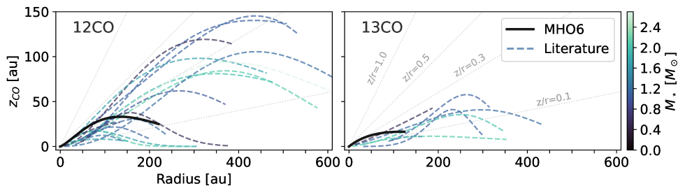
Figure 6: Line emission surface height of the MHO 6 disk compared to the fitted surfaces of ¹²CO and ¹³CO emission from Law et al. (2021b, 2022, 2023). Surfaces are only shown over their fitting range, while MHO 6 is shown until its $R_{95\%}$. The color of each line represents the mass of the central star.

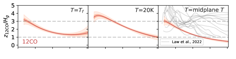
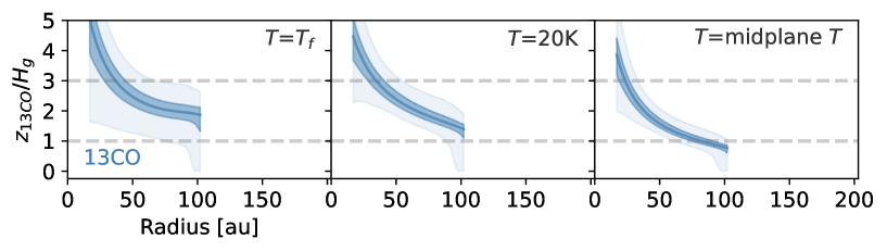
Figure 7: Ratio between the elevation of the emitting layer $z(r)$ over the expected pressure scale height $H_{g}$ for different midplane temperature prescriptions. Left: Temperature profile equal to the front layer temperature of each isotopologue. Middle: Temperature constant equal to 20 K. Right: Temperature follows Eq. 7. The darker and lighter shaded regions represent the $1\sigma$ and $3\sigma$ uncertainty of each profile, respectively. The gray lines in the top right panel show the $z/H$ ratio from the disks analyzed in Law et al. (2022).

5.2 Comparison of MHO6 with other sources

MHO 6 is the first very low mass star for which there is a direct measurement of the elevation of its emitting layer and brightness temperature as a function of its radii. In the following, we compare some of its measured properties to other disks that have been observed with ALMA.

The elevation of the emitting surface $z(r)$ of MHO 6 was modeled with the same functional form as in Law et al. (2022, 2023) in the image plane, which allows for a direct comparison of the results. The disks studied in those works are Class II sources with mid-inclination midplanes relative to the line of sight, covering a range of stellar masses from $0.5\,M_{\odot}$ to $2.7\,M_{\odot}$. In Fig. 6, we compare the elevation of the emitting surfaces of those disks to our measurement in MHO 6, which is the star with the lowest mass of the sample ($0.164\,M_{\odot}$ from ¹²CO). Within the first 50 au in radii, MHO 6 is among the most elevated emitting surfaces in both CO isotopologues when measured in distance from the midplane. This result is consistent with models which predicted disks around VLMS to be geometrically thicker due to the reduced force of gravity from the central star (Mulders & Dominik 2012; Sinclair et al. 2020). The ¹²CO emitting layer is at $z/r>0.3$ until a radii of 100 au, where it starts decreasing due to the more compact disk extension compared to the other sources.

Next, we investigated the ratio between the height of the emmitting surface and the gas pressure scale height $H_{g}$. As in Law et al. (2022), we describe $H_{g}$ as a function of radii under the assumption of vertical hydrostatic equilibrium, following:

$$H_{g}=\sqrt{\frac{k_{B}\,T_{\rm{mid}}\,r^{3}}{\mu\,m_{p}\,G\,M_{\star}}}\text{,}$$ (6)

where $k_{B}$ is the Boltzmann constant, $G$ the gravitational constant, $m_{p}$ is the mass of the proton, and $\mu$ the mean molecular weight of the studied species. The only unknown quantity is the value of $T_{\rm{mid}}$ as a function of radii; this is because the mass of the star, $M_{\star}$, is constrained by our model. For each CO isotopologue, we calculate three different $H_{g}$ as a function of radii, by considering different descriptions for the midplane temperature. First, we considered the temperature to be that of the isotopologue front layer, as an approximation of a vertically isothermal disk; second, we set the temperature to be constant equal to 20 K; and third, we assume the midplane temperature is described by the simplified expression for a passively heated, flared disk in radiative equilibrium (Kenyon & Hartmann 1987; Chiang & Goldreich 1997; D’Alessio et al. 1998; Dullemond et al. 2001), as in Law et al. (2022):

$$T_{\rm{mid}}\,=\,\left(\frac{\varphi L_{\star}}{8\pi r^{2}\sigma_{SB}}\right)^{1/4}\text{,}$$ (7)

where $\varphi$ is the flaring angle, which we set to 0.02 for comparison with the literature, $\sigma_{SB}$ is the Stefan-Boltzmann constant, and $L_{\star}$ is the stellar luminosity. By using $L_{\star}=0.06L_{\odot}$ from Kurtovic et al. (2021), derived from Herczeg & Hillenbrand (2014), Eq. 7 returns a $T_{\text{mid}}$ ranging between $20$ to $5$ K between the radii of $10$ to $150$ au, being the lowest of the three temperature descriptions.

Despite having one of the most elevated emission surfaces, MHO 6 shows one of the lowest ratios of $z/H_{g}$ among the sample of disks where this ratio has been measured, as shown in Fig. 7. For the ¹²CO emission, the main source of uncertainty to estimate the scale height of the emission layer comes from the $T_{\rm{mid}}$ assumption. Depending on the temperature prescription, we find that $z/H_{g}$ ranges from $1$ to $3\times H_{g}$. This estimate of an average $z/H_{g}\approx 2$ is consistent with the relations found in Law et al. (2022), where $z/H_{g}$ changes weakly with $M_{\star}$, and has a positive correlation with $R_{90\%}$. In the case of ¹³CO, the ratio $z/H_{g}$ is poorly constrained due to the uncertainty in $z_{13CO}(r)$, although the estimates appear to prefer the region of $1$ to $4\times H_{g}$ to a $1\,\sigma$ of uncertainty.

As expected for a very low mass star, MHO 6 shows a very low ¹²CO brightness temperature when compared to its more massive counterparts. At 100 au, the brightness temperature of the ¹²CO emission is $17\pm 1$ K, a few degrees lower than the coldest disk from the Law et al. (2022) sample (GW Lup, with $26\pm 0.5$ K at 100 au). However, the role of the optical depth in this measurement is still unclear, given that at 100 au the brightness temperature of the front and back layer becomes comparable (see Fig. 5).

5.3 Advantages of image- versus visibility-based analysis

Among the advantages of analyzing gas emission through parametric visibility modeling, the most notable is the incorporation of prior information on the model morphology. Typical image reconstruction methods, such as CLEAN, generate individual models for each channel without including information on the brightness distribution in the surrounding velocity channels. Consequently, the model of each channel is constrained by the individual channel sensitivity. This conservative approach is advantageous when the brightness distribution does not follow a characterizable spatially coherent structure in space and velocity, as observed in disks with strong Keplerian deviations, inflows, or outflows. However, it also limits the recovery of disk-like emission structures that are spread over many velocity channels. The generation of additional imaging products, such as moment maps, tends to limit the sensitivity of those collapsed images to be, at best, that of a single channel due to the cumulative effect of adding thermal noise. In contrast, prior assumptions over the emission morphology enable the characterization of faint structures that span several channels, substantially increasing the detection sensitivity.

The advantages that come with the implementation of a disk-like prior for the emission morphology can also be obtained through parametric image modeling. Previous works have used this approach to recover super-resolution structures in the inner disk from observations with high frequency resolution (e.g., Bosman et al. 2021), or to estimate deviations from expected pure Keplerian motion in the outer disk (e.g., Izquierdo et al. 2021). The difference between parametric image modeling and parametric visibility modeling comes in the stage at which the disk-like prior is assumed. In the image-based analysis, the prior is assumed after generating a model image for the visibilities of each channel. In a visibility-based analysis, the prior is assumed when generating the model image, thus preventing image reconstruction issues from influencing the model properties. Most of those issues are related to the beam convolution of CLEAN: (i) The beam convolution can artificially erase resolved emission structures that are well detected in the visibility plane (e.g., Andrews et al. 2021; Jennings et al. 2022); (ii) an inclined beam can modify the brightness distribution by enhancing the emission over the beam’s major axis; (iii) the emission can dilute within the beam if the beam area is larger than the emitting area, such as in the inner regions of the disk, leading to an underestimation of the brightness temperature; and (iv) faint large scale emission structures can be diluted in the noise background due to small beam sizes, even if the emission is detected in the visibilities (e.g., the outer ring of TW Hya, Ilee et al. 2022). Compared to the image plane, fitting in the visibility plane has the advantage of fitting uncorrelated noise. Although the inclined beam problem can be mitigated by forcing circularization of the point spread function (e.g., with visibility tappering, as in MAPS, Czekala et al. 2021), this circularization only increases the image spatial resolution loss. As for the dilution of emission in small and large scales, a typical imaging approach is to increase the weight towards more compact or extended baselines or to exclude specific ranges of the sampled visibilities. The visibilities, however, have the additive properties of the Fourier transform, and thus, excluding visibilities or modifying the weight given to them during the imaging process leads to further loss of total information. By creating and fitting a model in the visibility plane, the model must simultaneously fit all the visibility coverage, which mitigates issues related to spatial information loss and beam dilution. At the same time, the brightness distribution is controlled from the parametric model, avoiding biases from a non-symmetric visibility coverage.

Fitting all spatial scales covered by the visibilities with a disk morphology also has limitations. In an image-based approach, certain complex disk regions can be masked out of the fit, commonly isolating the outer or inner disk emission (e.g., Teague et al. 2021; Bosman et al. 2021, respectively), thus simplifying the models to focus them on a particular science case. Masking spatial regions is not possible with visibility modeling. As an example of adding complexity to a model, our visibility fitting of MHO 6 needed to include cloud contamination to the line emission as additional free parameters. If not accounted for, the model fitting would fit the cloud contribution by changing other disk parameters, such as the inclination or elevation of the emitting surface, thus misleading the recovery of disk information.

Another relevant comparative aspect of image versus visibility-based parametric modeling is their scalability with data volume. For a fixed frequency resolution, the fitted data volume in an image is determined by the image size and pixel size, as increasing the exposure time of the observation will result in higher image sensitivity, not in larger images. Further data volume reduction can be done by calculating the moment maps of the channels, which also allows for independent studies focused solely on the emission morphology or the kinematics. In the case of visibility analysis, increasing exposure time will continuously increase the fitted data volume due to the additive properties of the Fourier transform, and there is no feasible visibility simile to creating a moment map with the visibilities. Thus, a visibility model must describe intensity distribution and gas kinematics simultaneously. The selection of one method over another becomes dependent on the scientific goal. Overall, the advantages of visibility-based approaches are maximized when studying observations inaccessible to image-based techniques. One example is the recovery of the ¹³CO emission morphology of MHO 6 shown in Fig. 3, which despite being detected in several channels, does not allow for an image characterization of its structure due to the low S/N in each beam. Thus, emission detected with low sensitivity, or disk regions resolved by only a few resolution elements are the ideal study cases to be considered for visibility modeling.

5.4 How much nesting is needed

Increasing the level of nesting results in better pixel flux conservation in the inner disk, as exemplified in Fig. 13, where the flux ratio between a nested image of $n=6$ is compared to models with fewer levels of nesting. However, additional nesting levels come with additional computational cost. The acceptable flux loss should be decided on the basis of a comparison with an observation’s sensitivity, such that the dominant uncertainty source is the single channel sensitivity and not the model’s flux loss.

The level of nesting needed to model a specific observation will be dependent on the spatial resolution, frequency resolution, and disk properties. The main driver for flux loss during the construction of a parametric model is the undersampling of emitting regions in the inner disk, when the scale of brightness variations becomes smaller than the pixel size. This effect should be most significant for observations with very high-frequency resolution towards disks with high midplane inclinations or small line broadening in the line of sight.

In the case of the MHO 6, a pixel size of 15 mas is small enough to model the spatial frequencies covered in the visibilities, as the pixel is about seven times smaller than the angular resolution. However, as shown in Fig. 12 and Fig. 13, the inner 10 au can have a flux loss as large as 20% with this pixel size, which is about 0.2 Jy for the ¹²CO emission. Increasing the nesting level from $n=0$ to $n=2$ leads to a decrease in flux loss from 20% to 2%, which is about 0.022 Jy for the inner 10 au. By dividing over the 32 fitted channels, the nesting of $n=2$ leads to an average flux loss of $\sim 0.7$ mJy per channel, or $\sim 1.8$ K in brightness temperature considering that a region of 10 au is contained in a single beam. Thus, the flux loss is below $0.5\sigma$ per channel, and is below the profile noise level in the inner 10 au (see uncertainty in Fig. 5). Even though a nesting of $n=2$ is appropriate for this observation of MHO 6, the value of $n$ should be considered for every source and every observation separately.

An important consideration to determine $n$ is that the flux loss due to pixel undersampling is proportional to the total flux. Therefore, disks with very bright emission lines and high sensitivity observations could require a higher level of nesting compared to fainter disks observed at the same angular resolution, frequency resolution, and exposure time.

6 Conclusions

We present a novel method that uses parametric visibility modeling to analyze the emission profile of molecular lines obtained with interferometric millimeter observations of protoplanetary disks. To reach flux conservation with a non-prohibitive pixel size, we explored oversampling the central pixels using “nested images,” thereby increasing the flux fidelity of the models without using Monte Carlo-based radiative transfer methods. By remaining purely parametric, the modeling becomes rapidly iterable, which is key for testing different parametric combinations to describe the emission properties.

We applied this new method to the observations of ¹²CO and ¹³CO of the protoplanetary disk around the very-low-mass star MHO 6. Our method confirms the stellar mass of MHO 6 obtained in previous works (Kurtovic et al. 2021; Pegues et al. 2021), independently obtaining consistent results with each isotopologue. When compared to the sample of Law et al. (2022), we find the surface of MHO 6 to be among the most elevated surfaces in distance from the midplane within the first $50\,$au in radii. This is in agreement with the geometrically thicker morphology that is expected for disks around very-low-mass stars compared to Solar-type disks. We also recover the brightness temperature of the back emission layer in the ¹²CO emission, which is consistent with the freezing temperature of this molecule.

Using the emission of our models, we obtain the gas disk radii and confirm that the ratio of gas to dust size is around 4, which has been suggested as evidence of dust evolution through radial drift (Trapman et al. 2019). The emission in the ¹²CO shows evidence of a low-contrast non-azimuthally symmetric temperature distribution, which could be a result of an incomplete description of an optical depth effect.

The robustness of a parametric visibility modeling approach to analyzing the gas emission of protoplanetary disks is demonstrated with our fit to the ¹³CO emission. Despite the ¹³CO being compact in size, and only detected in a few channels with poor frequency resolution, our model recovers consistent results compared to the ¹²CO model, providing precise measurements and uncertainties for the emission morphology, size, and flux. Visibility modeling represents an alternative approach to analyzing those observations where image-based methods are not able to disentangle emission surfaces, directly recovering all the relevant properties of the disk for comparison with models of planet formation.

Appendix A Parametric visibility modeling results

The Figures showing the modeled cloud transparency and the moment maps for the ¹²CO observation and model are shown in Figs. 8 and 9, respectively. The best parameters of the ¹²CO and ¹³CO models are shown in Table 1.

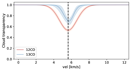
Figure 8: Cloud transparency for ¹²CO and ¹³CO emission. The shaded regions show the $1\sigma$ confidence levels. The systemic velocity from Table 1 is shown with a dashed line.

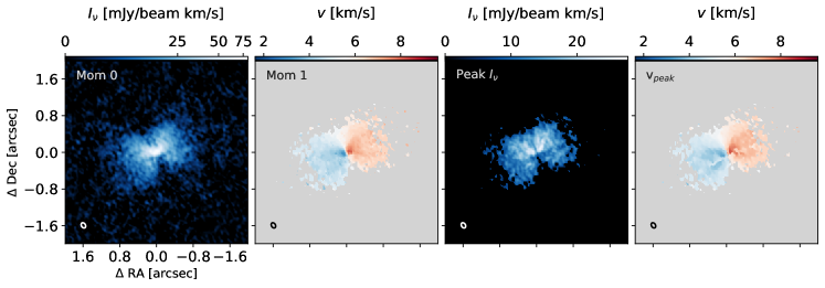
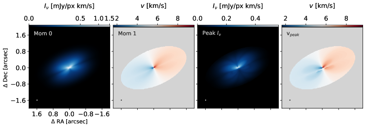
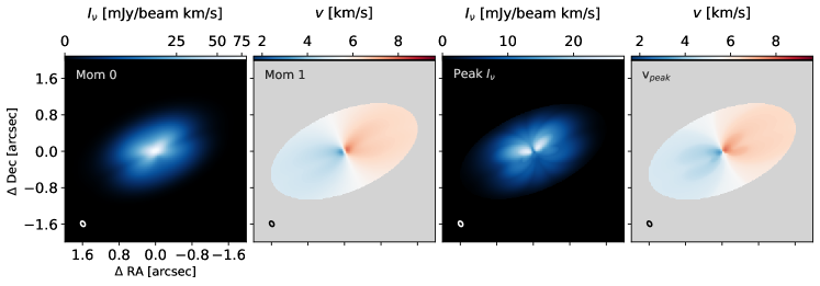
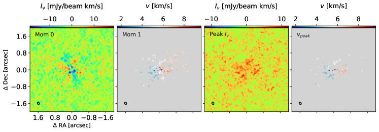
Figure 9: Moment maps of the ¹²CO emission. From top to bottom row: Moment maps of the ALMA observation, the best model with a nominal pixel resolution, the best model after beam convolution, and the residual images. All moment maps where generated using a Keplerian mask.

Table 1: Results of the MCMC fitting for the ¹²CO and ¹³CO emission of MHO 6. The uncertainties are measured from the 16th and 84th percentiles of each distribution. The fluxes ($F_{sky}$, $F_{corr}$) and the radii ($R_{68\%}$, $R_{90\%}$, $R_{95\%}$) are calculated from the models, and they are not free parameters.

Parameter	12CO	13CO	units	Parameter	12CO	13CO	units
$\delta_{\rm{RA}}$	$6.3_{-1.5}^{+1.0}$	$7.8_{-3.7}^{+3.3}$	mas	$I_{b}$	$0.36_{-0.03}^{+0.01}$	$0.17_{-0.04}^{+0.02}$	mJy/px
$\delta_{\rm{Dec}}$	$5.2_{-1.8}^{+1.3}$	$1.6_{-4.8}^{+5.1}$	mas	$\alpha_{b}$	$0.01_{-0.01}^{+0.01}$	$0.04_{-0.4}^{+0.23}$	-
inc	$59.1_{-0.5}^{+2.8}$	$59.6_{-1.4}^{+1.7}$	deg	$\beta_{b}$	$2.95_{-0.06}^{+0.38}$	$1.92_{-0.06}^{+0.69}$	-
PA	$293.5_{-0.3}^{+0.2}$	$293.8_{-0.9}^{+0.5}$	deg
$M_{\star}$	$0.164_{-0.003}^{+0.003}$	$0.171_{-0.010}^{+0.009}$	$M_{\odot}$	$\delta v_{0}$	$457.9_{-7.4}^{+6.6}$	$780.9_{-42.4}^{+48.3}$	m s-1
VLSR	$5627.0_{-3.6}^{+3.8}$	$5690.9_{-13.4}^{+13.4}$	m s-1	$q$	$0.40_{-0.02}^{+0.02}$	$0.15_{-0.05}^{+0.05}$	-
				$\delta v_{max}$	$<1371.4_{-44.5}^{+430.8}$	$<1466.7_{-309.5}^{+359.8}$	m s-1
$r_{z}$	$49.5_{-6.9}^{+46.8}$	$105.1_{-4.6}^{+138.3}$	au	$cl_{v0}$	$2.6_{-14.2}^{+14.4}$	$-6.1_{-72.6}^{+81.8}$	m s-1
$r_{I}$	$152.1_{-0.1}^{+3.5}$	$98.1_{-2.05}^{+10.0}$	au	$cl_{\sigma}$	$986.2_{-70.9}^{+77.1}$	$563.3_{-151.4}^{+180.9}$	m s-1
$r_{max}$	$<839.5_{-450.1}^{+49.5}$	$<578.3_{-287.0}^{+283.8}$	au	$cl_{a}$	$0.47_{-0.02}^{+0.02}$	$0.30_{-0.04}^{+0.07}$	-
$r_{cav}$	$1.6_{-0.9}^{+1.0}$	$4.2_{-1.2}^{+0.5}$	au				-
$z_{0}$	$205.2_{-60.9}^{+59.3}$	$24.7_{-3.7}^{+23.9}$	au	$F_{sky}$	$6.56_{-0.05}^{+0.05}$	$1.42_{-0.03}^{+0.04}$	mJy km s-1
$\psi$	$1.56_{-0.13}^{+0.10}$	$0.60_{-0.09}^{+0.15}$	-	$F_{corr}$	$9.68_{-0.38}^{+0.46}$	$1.59_{-0.07}^{+0.10}$	mJy km s-1
$\phi$	$0.87_{-0.10}^{+0.15}$	$19.15_{-18.08}^{+27.57}$	-
$I_{f}$	$0.42_{-0.03}^{+0.02}$	$0.09_{-0.01}^{+0.02}$	mJy/px	$R_{68\%}$	$131.2_{-1.8}^{+1.9}$	$72.4_{-4.3}^{+3.8}$	au
$\alpha_{f}$	$0.32_{-0.01}^{+0.03}$	$0.80_{-0.11}^{+0.05}$	-	$R_{90\%}$	$182.3_{-3.0}^{+3.0}$	$94.6_{-8.2}^{+8.7}$	au
$\beta_{f}$	$2.58_{-0.11}^{+0.13}$	$15.74_{-11.26}^{+3.76}$	-	$R_{95\%}$	$203.6_{-3.3}^{+3.2}$	$102.2_{-10.7}^{+11.9}$	au

Appendix B Alternative combination of emitting layers

Alternatively to Eq. 5, we experimented using a smooth transition from $I_{f,k}$ to $I_{b,k}$ with a power law weighting:

$$\centering I_{k}=\left\{\begin{aligned} I_{f,k}\,\text{,}&\,\,\,\,\,\text{for }I_{f,k}\geq\mu\\ I_{f,k}+\epsilon I_{b,k}\,\text{,}&\,\,\,\,\,\text{for }I_{f,k}<\mu\\ \end{aligned}\right.\text{,}\@add@centering$$ (8)

where $\mu$ is the threshold at which the emission of the front layer stops being completely optically thick, and $\beta$ is a function of range $[0,1]$ calculated in the region of interest as:

$$\centering\epsilon=1-\left(\frac{I_{f,k}}{\mu}\right)^{\gamma}\text{,}\@add@centering$$ (9)

thus, the combination is described with two free parameters, $\mu$ and $\gamma$. A fit to the ¹²CO data was done using this $(\mu,\gamma)$ approximation to combine the layers, with consistent results for $z_{f}$, $I_{f}$ and $I_{b}$ compared to Eq. 5. The best results were $\mu=0.355\pm 0.04$ mJy/px and $\gamma=0.3\pm 0.05$, but no significant change is seen in the residuals map, as shown in Fig. 10.

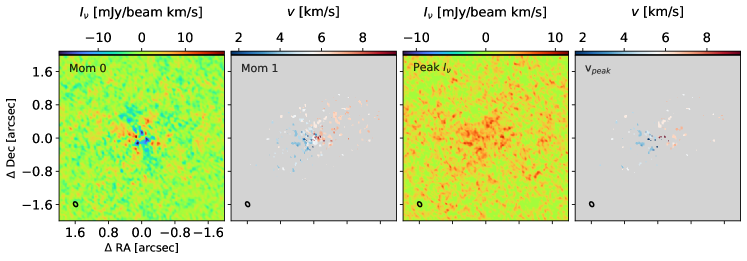
Figure 10: Moment maps of the residuals from the best model where the front and back layers where combined with Eq. 8. All moments where generated using a Keplerian mask.

Appendix C Nesting images

Figure 11: For a given velocity channel, the same model is shown with different nesting levels. All the nested images are then integrated into a reduced image, with the same pixel size for all of them. The lower row shows the residual between the reduced image generated with $n=6$ and models with lower $n$.

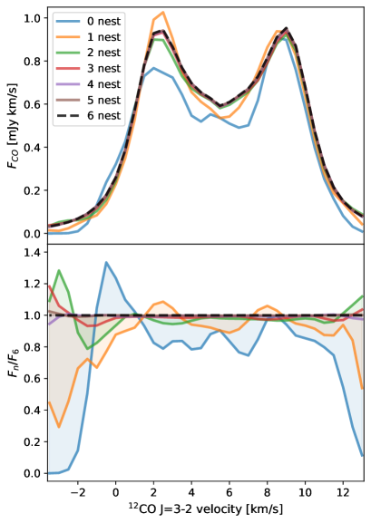
Figure 12: Flux variations as a function of velocity, for a disk of 10 au in size with the same model parameters as those from the ¹²CO of MHO 6. Upper panel: Total flux as a function of velocity for different nesting levels. Lower panel: Flux ratio between a model with $n=6$ and models with lower nesting level.

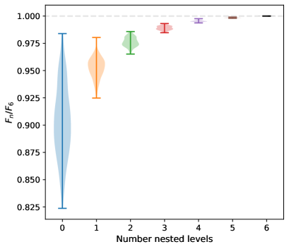
Figure 13: Distribution of flux ratio between models with different levels of nesting and a model with a nesting of $n=6$ as a reference. For each nested level, 256 models where generated by shifting the center of the disk by 1 mas in the RA and Dec grid, covering the full extent of one nominal pixel. For each nested level the width of the shape is representative of the density distribution of the sample.

The nesting image process is used to create model images with higher flux fidelity for the inner disk region, oversampling the nominal images by $4^{n}$, where $n$ is the level of nesting. In order to compare the flux difference between models with the same parameters but different nesting levels, we generate model images for a disk of 10 au in radius with similar model parameters to those of MHO 6 ¹²CO emission. The nominal pixel size is set to $15\,$mas, as in the ¹²CO fit.

We generated models from $n=0$ (no nesting) to $n=6$ (oversample each nominal pixel with $4^{6}$ pixels), and took the model images with $n=6$ as the reference for true flux. In Fig. 11, we show the residuals between each reduced image relative to the $n=6$ reduced image for a single channel. In Fig. 12, we show the total flux difference between $n=6$ and lower levels of nesting as a function of velocity. The models with $n=0$ and $n=1$ show the largest deviations from the true flux. In the lower panel of Fig. 12, the proportion between the flux of each model is compared to that of $n=6$, showing that even with $n=2$ or $n=3$, the channels with very faint emission could have discrepancies as large as 30% at high velocities. Thus, the nesting level has to be chosen so that those variations do not dominate the noise during the fitting process.

In order to investigate the impact of small spatial variations of the disk center relative to the pixel grid, we ran the same model with levels of nesting from $n=0$ to $n=6$, changing the disk center by 1 mas in RA and Dec until a full 15 mas offset was completed (the pixel size in the nominal image). This gave us a grid of 256 models per level of nesting. The flux variation is shown in Fig. 13, where it can be seen that spatial offsets of the disk center can change the total flux of the inner 10 au by a factor of $\sim 15\%$ when no nesting is being applied. Increasing $n$ has an asymptotic improvement over the flux conservation.

References

- Ables (1974) Ables, J. G. 1974, A&AS, 15, 383
- Andrews et al. (2021) Andrews, S. M., Elder, W., Zhang, S., et al. 2021, ApJ, 916, 51
- Andrews et al. (2018) Andrews, S. M., Huang, J., Pérez, L. M., et al. 2018, ApJ, 869, L41
- Bosman et al. (2021) Bosman, A. D., Bergin, E. A., Loomis, R. A., et al. 2021, ApJS, 257, 15
- Briggs (1995) Briggs, D. S. 1995, PhD thesis, New Mexico Institute of Mining and Technology
- Cárcamo et al. (2018) Cárcamo, M., Román, P. E., Casassus, S., Moral, V., & Rannou, F. R. 2018, Astronomy and Computing, 22, 16
- Casassus et al. (2006) Casassus, S., Cabrera, G. F., Förster, F., et al. 2006, ApJ, 639, 951
- Chiang & Goldreich (1997) Chiang, E. I. & Goldreich, P. 1997, ApJ, 490, 368
- Cieza et al. (2021) Cieza, L. A., González-Ruilova, C., Hales, A. S., et al. 2021, MNRAS, 501, 2934
- Clark (1980) Clark, B. G. 1980, A&A, 89, 377
- Cornwell & Evans (1985) Cornwell, T. J. & Evans, K. F. 1985, A&A, 143, 77
- Czekala et al. (2015) Czekala, I., Andrews, S. M., Jensen, E. L. N., et al. 2015, ApJ, 806, 154
- Czekala et al. (2021) Czekala, I., Loomis, R. A., Teague, R., et al. 2021, ApJS, 257, 2
- D’Alessio et al. (1998) D’Alessio, P., Cantö, J., Calvet, N., & Lizano, S. 1998, ApJ, 500, 411
- Dullemond et al. (2001) Dullemond, C. P., Dominik, C., & Natta, A. 2001, ApJ, 560, 957
- Flaherty et al. (2020) Flaherty, K., Hughes, A. M., Simon, J. B., et al. 2020, ApJ, 895, 109
- Flaherty et al. (2015) Flaherty, K. M., Hughes, A. M., Rosenfeld, K. A., et al. 2015, ApJ, 813, 99
- Foreman-Mackey et al. (2013) Foreman-Mackey, D., Hogg, D. W., Lang, D., & Goodman, J. 2013, PASP, 125, 306
- Gaia Collaboration et al. (2021) Gaia Collaboration, Brown, A. G. A., Vallenari, A., et al. 2021, A&A, 649, A1
- Hashimoto et al. (2021) Hashimoto, J., Dong, R., & Muto, T. 2021, AJ, 161, 264
- Hendler et al. (2020) Hendler, N., Pascucci, I., Pinilla, P., et al. 2020, ApJ, 895, 126
- Herczeg & Hillenbrand (2014) Herczeg, G. J. & Hillenbrand, L. A. 2014, ApJ, 786, 97
- Högbom (1974) Högbom, J. A. 1974, A&AS, 15, 417
- Ilee et al. (2022) Ilee, J. D., Walsh, C., Jennings, J., et al. 2022, MNRAS, 515, L23
- Izquierdo et al. (2022) Izquierdo, A. F., Facchini, S., Rosotti, G. P., van Dishoeck, E. F., & Testi, L. 2022, ApJ, 928, 2
- Izquierdo et al. (2021) Izquierdo, A. F., Testi, L., Facchini, S., Rosotti, G. P., & van Dishoeck, E. F. 2021, A&A, 650, A179
- Jennings et al. (2020) Jennings, J., Booth, R. A., Tazzari, M., Rosotti, G. P., & Clarke, C. J. 2020, MNRAS, 495, 3209
- Jennings et al. (2022) Jennings, J., Tazzari, M., Clarke, C. J., Booth, R. A., & Rosotti, G. P. 2022, MNRAS, 514, 6053
- Kenyon & Hartmann (1987) Kenyon, S. J. & Hartmann, L. 1987, ApJ, 323, 714
- Keppler et al. (2019) Keppler, M., Teague, R., Bae, J., et al. 2019, A&A, 625, A118
- Kurtovic et al. (2021) Kurtovic, N. T., Pinilla, P., Long, F., et al. 2021, A&A, 645, A139
- Kurtovic et al. (2022) Kurtovic, N. T., Pinilla, P., Penzlin, A. B. T., et al. 2022, A&A, 664, A151
- Law et al. (2022) Law, C. J., Crystian, S., Teague, R., et al. 2022, ApJ, 932, 114
- Law et al. (2021a) Law, C. J., Loomis, R. A., Teague, R., et al. 2021a, ApJS, 257, 3
- Law et al. (2021b) Law, C. J., Teague, R., Loomis, R. A., et al. 2021b, ApJS, 257, 4
- Law et al. (2023) Law, C. J., Teague, R., Öberg, K. I., et al. 2023, ApJ, 948, 60
- Long et al. (2022) Long, F., Andrews, S. M., Rosotti, G., et al. 2022, ApJ, 931, 6
- Long et al. (2021) Long, F., Andrews, S. M., Vega, J., et al. 2021, ApJ, 915, 131
- Long et al. (2018) Long, F., Pinilla, P., Herczeg, G. J., et al. 2018, ApJ, 869, 17
- Loomis et al. (2018) Loomis, R. A., Öberg, K. I., Andrews, S. M., et al. 2018, AJ, 155, 182
- McMullin et al. (2007) McMullin, J. P., Waters, B., Schiebel, D., Young, W., & Golap, K. 2007, in Astronomical Society of the Pacific Conference Series, Vol. 376, Astronomical Data Analysis Software and Systems XVI, ed. R. A. Shaw, F. Hill, & D. J. Bell, 127
- Mulders & Dominik (2012) Mulders, G. D. & Dominik, C. 2012, A&A, 539, A9
- Narayan & Nityananda (1986) Narayan, R. & Nityananda, R. 1986, ARA&A, 24, 127
- Öberg et al. (2021) Öberg, K. I., Guzmán, V. V., Walsh, C., et al. 2021, ApJS, 257, 1
- Paneque-Carreño et al. (2023) Paneque-Carreño, T., Miotello, A., van Dishoeck, E. F., et al. 2023, A&A, 669, A126
- Pegues et al. (2021) Pegues, J., Czekala, I., Andrews, S. M., et al. 2021, ApJ, 908, 42
- Pinilla (2022) Pinilla, P. 2022, European Physical Journal Plus, 137, 1206
- Pinte et al. (2018) Pinte, C., Ménard, F., Duchêne, G., et al. 2018, A&A, 609, A47
- Ponsonby (1973) Ponsonby, J. E. B. 1973, MNRAS, 163, 369
- Qi et al. (2013) Qi, C., Öberg, K. I., & Wilner, D. J. 2013, ApJ, 765, 34
- Schwarz et al. (2016) Schwarz, K. R., Bergin, E. A., Cleeves, L. I., et al. 2016, ApJ, 823, 91
- Sinclair et al. (2020) Sinclair, C. A., Rosotti, G. P., Juhasz, A., & Clarke, C. J. 2020, MNRAS, 493, 3535
- Tazzari et al. (2017) Tazzari, M., Testi, L., Natta, A., et al. 2017, A&A, 606, A88
- Teague (2019) Teague, R. 2019, The Journal of Open Source Software, 4, 1220
- Teague (2019) Teague, R. 2019, Research Notes of the American Astronomical Society, 3, 74
- Teague (2022) Teague, R. 2022, wrinkleology, https://github.com/richteague/wrinkleology
- Teague et al. (2021) Teague, R., Bae, J., Aikawa, Y., et al. 2021, ApJS, 257, 18
- Trapman et al. (2019) Trapman, L., Facchini, S., Hogerheijde, M. R., van Dishoeck, E. F., & Bruderer, S. 2019, A&A, 629, A79
- Ward-Duong et al. (2018) Ward-Duong, K., Patience, J., Bulger, J., et al. 2018, AJ, 155, 54
- Wölfer et al. (2023) Wölfer, L., Facchini, S., van der Marel, N., et al. 2023, A&A, 670, A154
- Zawadzki et al. (2023) Zawadzki, B., Czekala, I., Loomis, R. A., et al. 2023, PASP, 135, 064503
- Zhang et al. (2021) Zhang, K., Booth, A. S., Law, C. J., et al. 2021, ApJS, 257, 5