Interactive Learning of Physical Object Properties Through Robot Manipulation and Database of Object Measurements

Abstract

This work presents a framework for automatically extracting physical object properties, such as material composition, mass, volume, and stiffness, through robot manipulation and a database of object measurements. The framework involves exploratory action selection to maximize learning about objects on a table. A Bayesian network models conditional dependencies between object properties, incorporating prior probability distributions and uncertainty associated with measurement actions. The algorithm selects optimal exploratory actions based on expected information gain and updates object properties through Bayesian inference. Experimental evaluation demonstrates effective action selection compared to a baseline and correct termination of the experiments if there is nothing more to be learned. The algorithm proved to behave intelligently when presented with trick objects with material properties in conflict with their appearance. The robot pipeline integrates with a logging module and an online database of objects, containing over 24,000 measurements of 63 objects with different grippers. All code and data are publicly available, facilitating automatic digitization of objects and their physical properties through exploratory manipulations.

Figure 1: Exploratory action selection to estimate object properties – schematic overview. Using the current belief, next action is selected to maximize the expected Information Gain (IG), taking the uncertainty of each action into account. After each action, new belief is computed using inference of Bayesian Network, and new action is selected.

I Introduction

While rapid progress is being made in automatically extracting information about objects from large image datasets and text corpora, estimating physical properties remains a challenge. This work paves the way to automatic extraction of physical object properties such as material composition, mass, volume or stiffness, which typically require physically manipulating the object. We present a theoretical framework and its experimental evaluation that deals with exploratory action selection to maximize what can be learned about objects on the table in front of a robot manipulator. In our demonstrator, there is a partially adversarial mix of 17 household objects of different shapes and from different materials (incl. a real and a plastic banana, wine glass from glass and plastic, a soft and a hard sponge with identical appearance), 6 object properties (2 discrete – category and material; 4 continuous – elasticity, density, volume, and mass), and 5 actions the robot system can perform (2 based on vision – estimate the category or material from the image; 3 manipulation actions – squeeze, poke, and lift). We expressed the conditional dependencies between the properties using a Bayesian Network (BN) (see Fig. 2 and added freely available prior probability distributions as well as uncertainty associated with different measurement actions. After specifying which object property should be estimated, our algorithm chooses the best exploratory action based on expected IG, updates all object properties using inference in the BN, and picks the next optimal action to be executed. We demonstrate that the overall average performance of the system outperforms a baseline and analyze interesting runs showing how the algorithm automatically and efficiently discovers object properties. The robot pipeline is integrated with a logging module and an online database of objects, currently containing more than 24000 measurements of 63 different objects using four different grippers. We make publicly available all code and data, which provides a starting point for automatic digitization of objects and their physical properties by exploratory manipulations.

Task and motion planning for robot manipulation, including sequences of actions, has been extensively studied using symbolic and recently also neuro-symbolic or neural approaches. In this work, the goal is not to perform a task (e.g., stack objects) but to learn about the properties of objects. Embodied reasoning for discovering object properties via manipulation was used in [1]; correct execution of a verbally specified task (e.g., stack objects by weight) required specific actions to learn about physical object properties. In this work, the order of actions is chosen not as to produce a cumulative result in the environment, but so that the action chosen next is optimal with respect to what can be learned about the object in front of the robot.

Active manipulation for perception can be non-prehensile (e.g. “push to know” [2, 3]) or prehensile, i.e. grasping the object or exploring it with robot fingers (e.g., [4]). In most cases, manipulation serves object localization, shape reconstruction, or recognition; learning physical object properties has been less studied [5]. Haptic exploration of physical object properties using several actions and sensory modalities is extremely rare ([6] a notable exception). The exploratory movements are typically chosen based on some form of probabilistic model and information theoretic measures like entropy or IG (see e.g., [7]).

An accompanying video is at https://youtu.be/h_ZIYUmzv-8; the code used in this work is available at https://github.com/ctu-vras/actsel; The object database and source code are available at https://cmp.felk.cvut.cz/ipalm/.

II Exploratory Action Selection Driven by Information Gain

Our method is based on a Bayesian Network (BN). Beliefs about each of the variables can be updated through measurements. The action-to-node relation can be found in Fig. 2. The BN consists of five nodes ordered by their enumerability types. (i) categorical (enumerable): Category and Material; (ii) continuous (non-enumerable): Elasticity, Density, and Volume. Discrete variables are represented with a Probability Mass Function (PMF); continuous variables with a Probability Density Function (PDF).

We consider 10 object Categories: bottle, bowl, box, can, dice, fruit, mug, plate, sodacan, wineglass.

We consider 8 Material classes: ceramic, glass, metal, soft plastic, hard plastic, wood, paper, foam.

Elasticity is a continuous variable expressed in Young’s modulus [kPa], Density in homogeneous density [kg/$m^{3}$], and Volume in the volume of the object’s material in [m³].

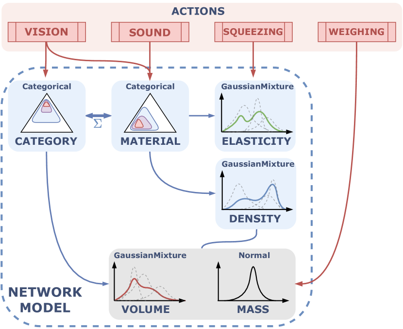
Figure 2: Bayesian Network Structure.

II-A Initialization

To establish initial beliefs for each property, first, a uniform PMF is set up for Category and Material. Those in turn initialize each continuous variable expressed by the relationships in the BN (Fig. 2), as shown in Fig. 3, giving rise to a Gaussian Mixture Model (GMM) for each continuous variable.

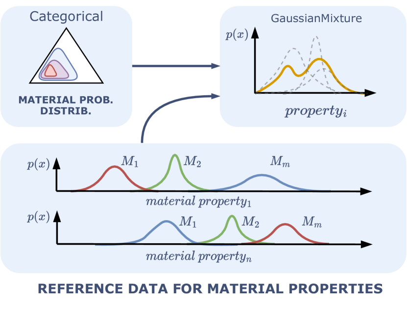
Figure 3: Initialization of GMM from the reference data by weighting by corresponding probability mass function.

The Category PMF is translated into the Volume PDF through the values in Table I. The Material PMF is translated into the Elasticity and Density PDFs through the means and Standard Deviations in Table II, extracted from technical literature [8, 9, 10, 11].

Volume [cm3]	Bottle	Bowl	Box	Can	Dice
	$30\pm 50$	$40\pm 80$	$10\pm 26$	$8\pm 60$	$37\pm 50$
	Fruit	Mug	Plate	Sodacan	Wineglass
$155\pm 28$	$97\pm 27$	$0\pm 15$	$5\pm 10$	$85\pm 20$

TABLE I: Reference values for Volume. The values are means and Standard Deviations (SDs) scraped from an online store.

	Ceramic	Glass	Metal	Soft Plastic
Density [kg$\cdot$ m-3]	$2300\pm 100$	$2600\pm 200$	$7900\pm 600$	$1300\pm 300$
Elasticity [kPa]	$150\pm 10$	$140\pm 10$	$130\pm 10$	$55\pm 30$
	Hard Plastic	Wood	Paper	Foam
Density [kg$\cdot$ m-3]	$1500\pm 300$	$646\pm 183.6$	$756.8\pm 223.8$	$91.9\pm 127.7$
Elasticity [kPa]	$75\pm 30$	$120\pm 10$	$35\pm 28$	$10\pm 15$

TABLE II: Reference values for density and elasticity. The values are means and Standard Deviations (SDs) extracted from the literature.

The conditional dependence between Category and Volume as well as the covariance matrix linking Category and Material were initialized using data extracted from the text descriptions of products available at an online store.

II-B Inference

Following the execution of an action, the network is updated based on the obtained results (measurement update). These data points are then incorporated as a product into the distribution of the given property. For categorical properties, the posterior distribution post-update is propagated to all other nodes in the BN, adhering to the network’s connections as an undirected graph. This updating process, known as message passing, involves transmitting message vectors between nodes. The format and order of these message vectors correspond to the relevant probability functions: for interactions between nodes related to Material, the format aligns with the material PMF, while for other interactions, it aligns with the category PMF.

When the message originates from a continuous property node, such as Elasticity, the continuum must be first transformed into a finite vector to align with the required message format. Given our knowledge of the original reference distribution of materials for Density, we only need to estimate the weights of the GMM using the Expectation–maximization (EM) algorithm. This approach allows the classification of unknown objects into material categories without necessitating a class for every known material. Consequently, objects that fall between two classes can be represented, for instance, as a blend, like $0.5\times property_{1},0.5\times property_{2}$. Subsequently, this message vector from Elasticity serves as a virtual measurement for the Material node. Posterior probabilities are computed using a confusion matrix to simulate the uncertainty inherent in message passing. Specifically, this confusion matrix is unique to each connection between nodes; it is computed beforehand at the initialization step from the reference data for every blue arrow in the network model depicted in Fig. 2.

When the message originates from a categorical property, i.e., a vector, the estimation step is bypassed, and message passing occurs directly from the product of the measurement vector and the associated confusion matrix.

II-C Measurement Models

The action selection algorithm needs to estimate the consequences of performing different actions, i.e. measurements. A measurement model, i.e. the accuracy of every measurement is required. For categorical variables, confusion matrices are used to compute the expected measurement. For brevity, only the average accuracy for each categorical action is given. Complete confusion matrices are available in the code repository. For continuous variables, a measurement is modeled as a normal distribution. The measurement accuracies and SDs are provided in the Table III. The SD for density was experimentally obtained based on the average performance of extracting a correct density belief from a mass measurement and a volume belief on the available experimental data. The mass measurement with our experimental setup has an accuracy of $\pm$ 6 [grams] for up to a 1 [kg] payload.

Action	Target node	Accuracy	SD $\sigma$	Units
mat-vision	Material (categorical)	0.2431	-	-
mat-sound	Material (categorical)	0.1002	-	-
cat-vision	Category (categorical)	0.6345	-	-
weighing	Density (continuous)	-	223	[kg$\cdot$m-3]
squeezing	Elasticity (continuous)	-	10	[kPa]

TABLE III: Measurement accuracy. Accuracies and Standard Deviations (SDs) from experimental data.

II-D Expected Information Gain

In our framework, IG quantifies the reduction in entropy of the probability distribution of one or more variables in our BN after executing an action. It reflects how much information the action and its associated measurement have provided. When we compute the difference in entropy before and after conducting an action, we refer to it as experimental or true IG. While experimental IG offers insight into the performance of an algorithm, by definition, it alone cannot be used to decide which action to take. Therefore, to guide the decision-making, one must create an emulation—an estimation of how the property distribution will likely appear after each action—to choose the action most likely to reduce entropy, thus increasing IG. The experimental IG is formalized as:

$$\Delta H(\nu)=H(\nu_{k})-H(\nu_{k+1}),$$ (1)

where $\nu$ represents a distribution of a node, either continuous or categorical (e.g., Elasticity: PDF or Category: PMF), $\Delta H(\nu)$ denotes the experimental IG, which is the difference in entropies. Here, $H(\nu{{}_{k}})$ is the entropy of a node distribution at algorithm iteration $k$, representing the prior, and $H(\nu_{k+1})$ is the entropy of the same node distribution at the next iteration step $k+1$, representing the posterior after the measurement. The expected IG is formalized as follows

$$\mathbb{E}[\Delta H(\nu)]=H(\nu_{k})-\mathbb{E}[H(\bar{\nu_{k}})],$$ (2)

where $\mathbb{E}[\Delta H(\nu)]$ is the expected IG, and $\mathbb{E}[H(\bar{\nu_{k}})]$ is the expected entropy of the posterior distribution, which is the entropy of the emulation. Note that the emulation also contains the index $k$, not $k+1$, to emphasize that it reflects only an expectation of the posterior based on the current belief. For the continuous properties, theoretically, the emulation could involve sampling infinitely many possible scenarios of the action measurements based on the probability density function of a given property. However, such an approach would require simulating Bayesian updates for a large number of samples, which consumes considerable CPU time. Since the variance of the action related to a given property is available, we chose a more efficient option—convolving the continuous prior probability density function of a given property $\nu_{k}$ with a normal distribution having a zero mean and variance equal to the variance of the action measurement in question $\mathcal{N}(0,\sigma_{a}^{2})$. This procedure propagates the expected error across the entire continuous probability density function of the property. Formally:

$$\bar{\nu_{k}}=\nu_{k}\ast\mathcal{N}(0,\sigma_{a}^{2}).$$ (3)

Subsequently, the expected continuous entropy is numerically calculated as:

$$\mathbb{E}[H(\bar{\nu_{k}})]=-\sum_{\mathcal{X}}h_{\mathcal{X}}\bar{\nu_{k}}(x)\log_{2}\bar{\nu_{k}}(x),$$ (4)

where the entropy is computed for each step on the support $\mathcal{X}$ of the property distribution. $h_{\mathcal{X}}$ denotes the normalization factor, determined by the bin size used for computing the sum-integral approximation. Strictly mathematically speaking, the Eq. (4) provides an integral approximation.

To represent the variance of the measurements for categorical properties, such as the Category vision module, the confusion matrix is employed. From this confusion matrix, a sample entropy vector is computed to create a categorical equivalent of the emulation in Eq. (3). Each element of the sample entropy vector at index $i$ is computed as

$$H(\bar{\nu_{k}}|m_{i})=-\sum_{j}C_{a}(i,j)\log_{2}C_{a}(i,j),$$ (5)

where $C_{a}$ is a row-unit-sum confusion matrix corresponding to action $a$, $m_{i}$ signifies the $i$-th member of the categorical property, e.g. ceramic for the Material node or a mug for the Category node. In the case of a column-unit-sum confusion matrix, the indices $(i,j)$ in Eq. (5) would interchange. To compute the expected entropy of the emulation, we use the resultant vector from Eq. (5) as:

$$\mathbb{E}_{m}[H(\bar{\nu_{k}})]=\sum_{m_{i}}C_{a}\nu_{k}(m_{i})H(\bar{\nu_{k}}|m_{i}),$$ (6)

where the result is a sum of the sample entropy vector weighted by an expected measurement computed as a matrix multiplication of the prior distribution and confusion matrix as $C_{a}\nu_{k}$. The result Eq. (6) is then substituted into Eq. (2) to obtain the expected IG.

II-E Action Selection Algorithm

The approach is schematically illustrated in Fig. 1 and the pseudo-algorithm is shown in Alg. 1. Formally, the optimal exploratory action is chosen as:

$$a^{*}=\text{argmax}_{a\in\mathcal{A}}\mathbb{E}[\Delta H(\nu|a)],$$ (7)

where $a$ is a specific action from the total set of available actions $\mathcal{A}$, and $a^{*}$ is the optimal action that maximizes the expected IG.

1

2for k in iterations do

3       $\eta_{k}:=\text{getNetworkEntropy}(N)$

4       for a $\in\mathcal{A}$ do

5             $\nu_{k,a}:=\nu_{k}\in N\;|\;a\rightarrow\nu_{k}$

6             $\overline{\nu_{k}}:=\text{emulatePosterior}(\nu_{k,a},a)$

7             $\mu_{k}:=\text{generateMessages}(\overline{\nu_{k}})$

8             $\overline{N}:=\text{propagateMessages}(N,\mu_{k})$

9             $\overline{\eta_{k}}:=\text{getExpectedNetworkEntropy}(\overline{N})$

10             $\mathbb{E}_{k}[\Delta H(N)]:=\eta_{k}-\overline{\eta_{k}}$

11            

12       end for

13      $a_{k}^{*}\in\textit{argmax}_{a\in\mathcal{A}_{k}}\mathbb{E}_{k}[\Delta H(N)]$

14      

15 end for

Algorithm 1 Action selection (ACSEL)

III Objects, Robot Setup, Action Repertoire

The setup and robot actions are illustrated in the accompanying video at https://youtu.be/h_ZIYUmzv-8.

III-A Manipulated Objects

We selected 17 objects, most of them from the YCB dataset [12], to be diverse in size, weight, volume, and material composition—see Fig. 4. We also included “trick” or adversarial objects where their material composition does not correspond to the best guess from their appearance (real and plastic bananas, a soft sponge and an identical but hardened sponge, wine glass from glass or plastic).

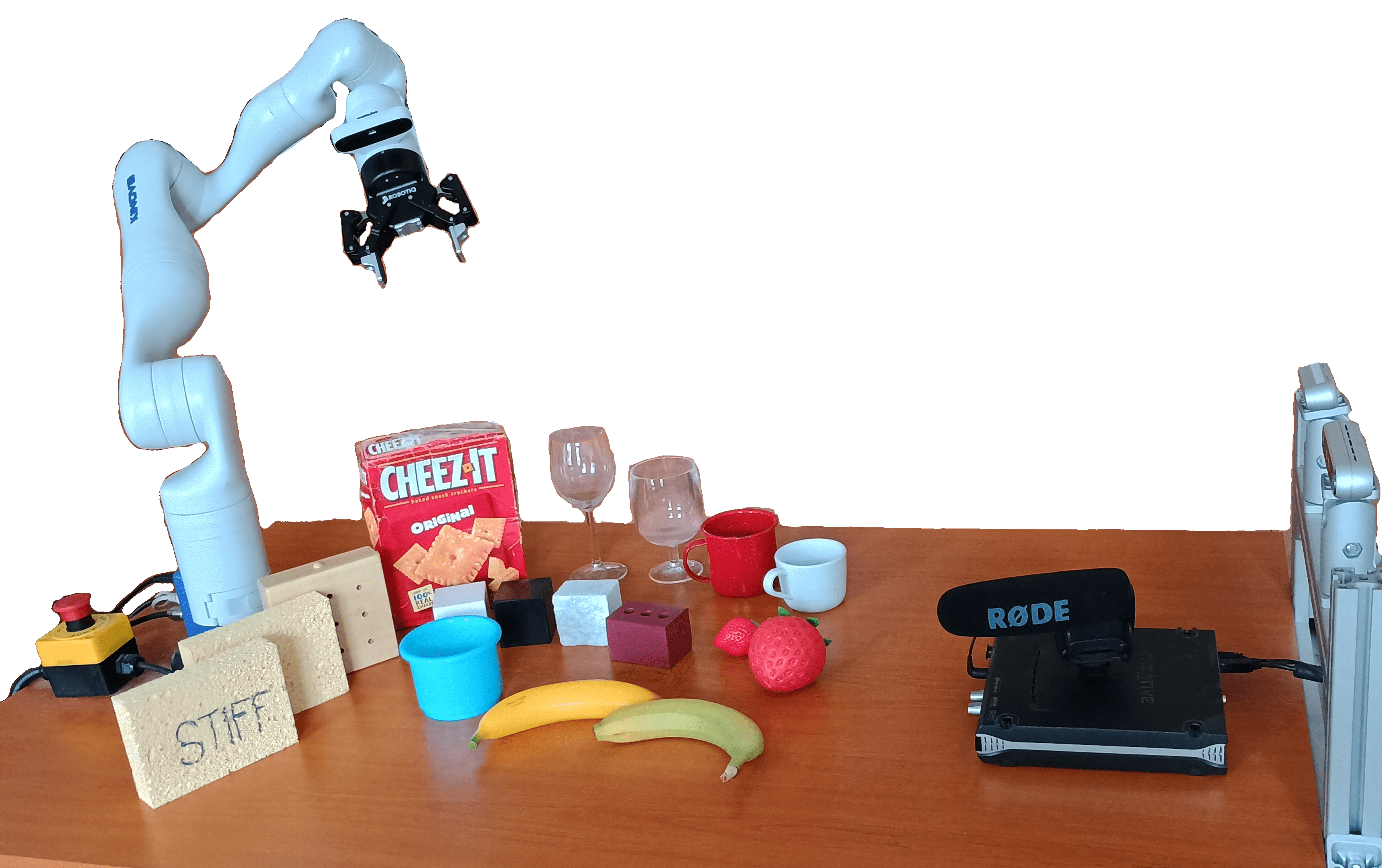
Figure 4: All 17 objects used and experimental setup. Kinova Gen3 robot, Robotiq 2f-85 gripper, Rode VideoMic Pro microphone, and RealSense D435 camera (on the right; only the RGB from one camera was used).

III-B Robot Setup

The real-world robot setup (Fig. 4) consisted of a Kinova Gen3 robotic manipulator (7 degrees of freedom), equipped with a Robotiq 2f-85 gripper used for squeezing and weighing actions. In addition, the gripper was used to poke objects to generate sounds for material classification (mat-sound). For this purpose, a professional shotgun microphone Rode VideoMic Pro was used. RGB images from a RealSense D435 camera were used for the measurements relying on vision (cat-vision, mat-vision).

III-C Action Repertoire

Weigh. The mass of objects is estimated by lifting them using the robot arm using torque measurements in the robot’s joints in a configuration where a certain robot joint axis is perpendicular to the force of gravity. The torque in this joint $\tau_{m}$ can be described by the formula $\tau_{m}=mgl+\tau_{0}$, where $m$ is the object mass, $l$ is the effective lever from the joint axis to the object center of mass, and $g$ is the gravitation constant, and $\tau_{0}$ is a reference torque recorded by moving the robot to the measuring pose while the gripper is empty.

Squeeze. Grasping or squeezing the object between the jaws of a parallel gripper provides force and displacement data—the stress-strain response of every object. We adapted the module we developed in [13] and approximated the stress-strain curve with a line—a coarse approximation of the object’s stiffness.

Material from sound. We used sound generated by poking the object with the closed gripper jaws to recognize the material. Audio recordings from the interactions were preprocessed and converted to grayscale melodic spectrograms and then fed into a modified ResNet34 network, with output labels representing the material classes. More details can be found in [14].

Material and Category from Vision. We used the Detectron2 algorithm [15] with R50-FPN backbone and trained the model using our dataset consisting of objects from the YCB dataset [12], SHOP-VRB [16] and our own generated in Unity.

IV Experiments and Results

In our experiments, one of 17 objects was placed in front of the robot. There were 5 actions or measurements (cat-vision, mat-vision, mat-sound, weighing, squeezing) in the repertoire that could be selected by our algorithm based on their expected IG, i.e. their likelihood to maximally reduce the uncertainty in one or more of the object properties. There were five object properties (2 discrete variables with PMF – Category and Material; 3 continuous with PDF – Elasticity, Density, Volume/Mass)—see Fig. 2 for an overview. The action/measurement informing the Category node was cat-vision; mat-vision or mat-sound could be employed to update the Material node; squeezing measured Elasticity. Density and Volume nodes did not have a corresponding measurement that would update them directly and relied on relationships within the BN.

The actions were selected “without replacement”, i.e. once a particular action was chosen, it was not available in the next step of the algorithm. Thus, with 5 actions in the repertoire, there were at most 5 algorithm steps. After every measurement, the BN was updated as explained in Section II-B. We ran two variants of the experiments: (a) with no stopping criterion—5 actions were always executed; (b) with stopping—if at a given algorithm step, there was no action available with positive expected IG, the algorithm would terminate. There were 5 runs of the algorithm for every object.

Optimization modes. To drive the action selection, one of the nodes could be selected for which the uncertainty should be reduced (say the user is interested in a specific object property). For Category or Material, the expected discrete IG for every action was be evaluated and the best action executed. For the continuous variables (Elasticity, Density, Volume), the corresponding differential IGs were evaluated. We have also assessed runs optimizing Category and Material together or the three continuous property nodes together. Aiming to reduce uncertainty in all five nodes at the same time would require adding the discrete and differential IG which is not mathematically rigorous, so this regime was not evaluated. Please note that all actions have their associated measurement models, i.e. the system has an estimate of the noise associated with every action. Thus, optimizing one property does not always lead to executing the action that directly measures that property.

IV-A Qualitative Illustration of the System’s Operation

The operation of the system is illustrated in Fig. 5 on three selected objects. In the first row (Panels A1-A4), the YCB wineglass, which is plastic, is explored while the Category variable is optimized. Cat-vision has the highest expected IG (panel A2) and is always chosen (panel A3). In the single run (panel A2), additional steps of the algorithm are shown. However, in this particular run, if termination was on, no more action would be executed as all actions have negative expected IG at step 1. Panel A4, right, shows the correct identification of the object Category as wineglass.

The other two rows show exploration of a sponge—a hardened exemplar in the middle (B1-B4) and a soft one at the bottom (C1-C4) (see accompanying video at https://youtu.be/h_ZIYUmzv-8);, in both cases with learning about Elasticity as the objective. Although the goal was to learn about the object stiffness, Cat-vision was chosen as the first most informative action to serve this objective. The squeezing action executed in the next step (see B2 and B3) adds information about the object being stiff, as is apparent in the final elasticity distribution as well as the material distribution (B4 vs. C4).

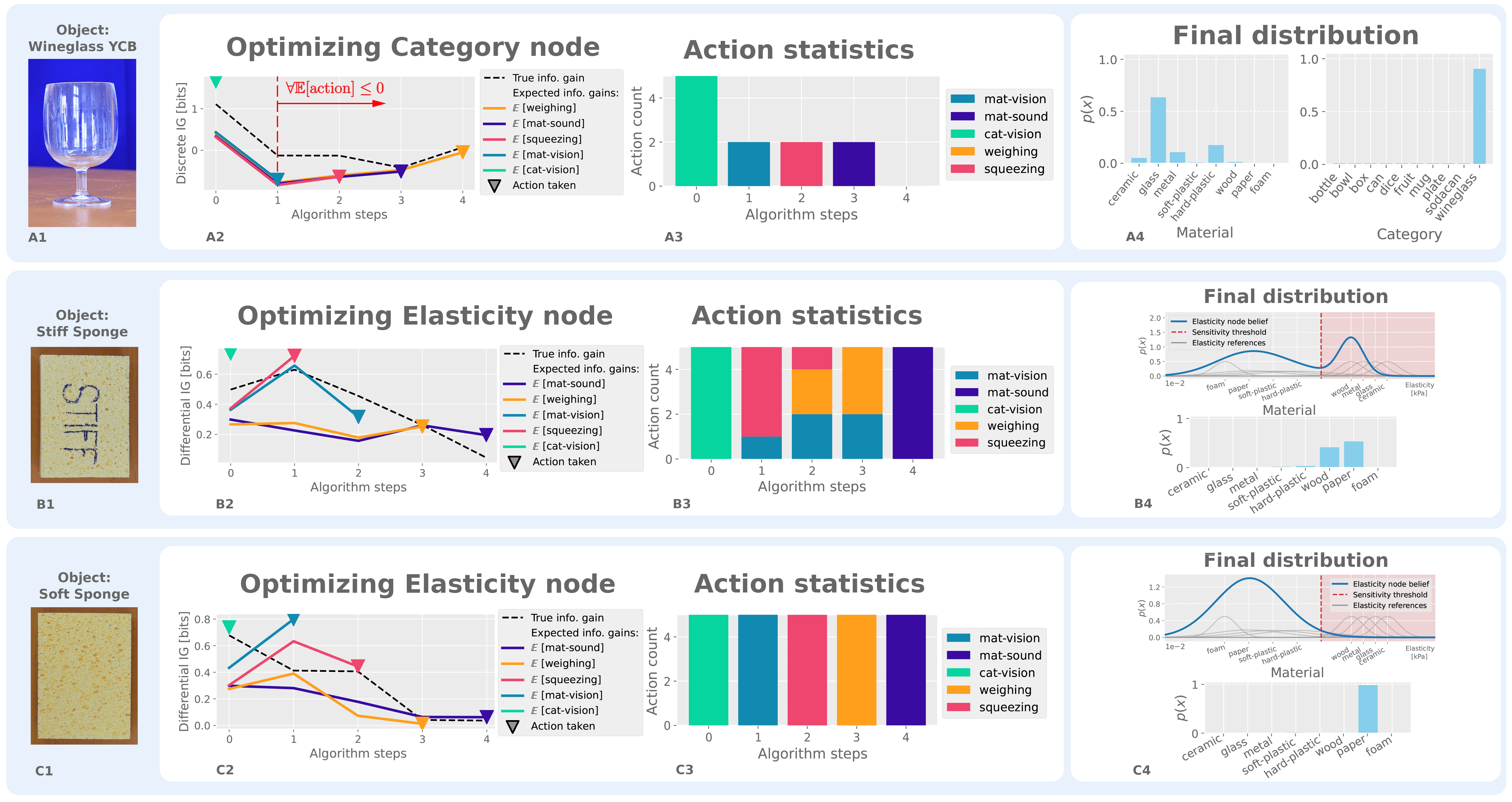
Figure 5: System operation and performance – examples. (Left – A1/B1/C1) Object name and image. (A2/B2/C2) Single run of experiment with termination criterion off. Expected IG of the actions shown. Triangle markers show which action was chosen in a given step. The dashed black line shows the experimental true IG after the action was executed. This action is not shown anymore in subsequent algorithm steps. (A3/B3/C3) Count of actions chosen during the runs with the termination on (if all available actions at a given step had negative expected IG, execution stopped). (A4/B4/C4) Probability distributions of relevant variables of the single run shown in (A2/B2/C2).

IV-B Action Statistics and Intelligent Exploration Termination

Fig. 6 shows how many times different actions were executed when different object properties, i.e. different nodes in the BN, were selected to be “learned about”. When reducing the uncertainty in the Category node is the target, Panel A shows that cat-vision was always selected as the first action. In about half the cases, the algorithm then terminated. In the other cases, mat-vision was picked in the second step. When asked to learn about the Material (Panel C), interestingly, the algorithm picked the Weighing action as the most effective in all cases, rather than the mat-vision or mat-sound actions that directly target the Material node through their measurement update. This illustrates how the algorithm automatically takes the complete BN and the measurement uncertainties into account. For the continuous variables (Panels B, D), the algorithm typically performed all five actions. Cat-vision wass the most informative action to learn about Category (Panel A), Elasticity (B), and all the continuous together variables (D) but not about Material (C).

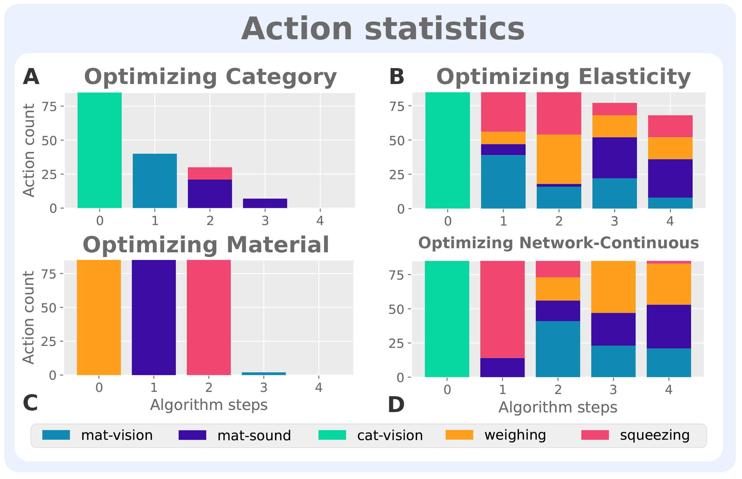
Figure 6: Action statistics. Running the algorithm in the active termination mode across all objects, 5 repetitions each. The bar plots show the count of actions selected at every step. Shorter bars indicate that some runs terminated as there was no action with positive expected IG. Optimizing Network-Continuous jointly optimizes all the continuous variables in the BN.

IV-C Average performance across all objects

To demonstrate the effectiveness of the proposed algorithm over all the objects, we ran the algorithm with 5 repetitions on each of the 17 objects, using the action selection algorithm proposed optimizing the Category node and with random action selection as a baseline (i.e., 2 action selection regimes x 17 objects x 5 repetitions x 5 algorithm steps). For comparison purposes, the termination check was off. Fig. 7 shows the average entropy of the Category variable after 5 steps of the algorithm in the two action selection regimes, including the variance. The intelligent action selection (ACSEL) outperforms RAND. Furthermore, in the ACSEL regime, the plot shows a dramatic drop in entropy after the execution of the first action/measurement, demonstrating that the most effective action was chosen in the first step for the majority of the objects.

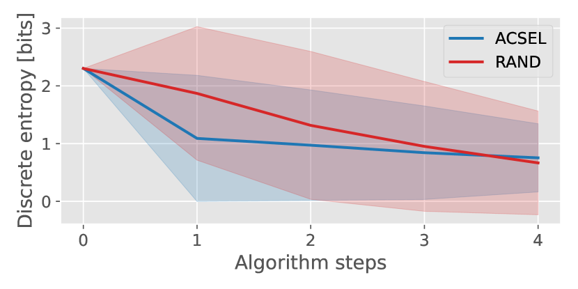
Figure 7: Average entropy (lower is better) of the Category node – Optimizing Category, 17 objects, 5 repetitions each. Comparing action selection based on IG (ACSEL) and random action selection (RAND).

To complement the analysis in Fig. 8 that shows entropy, which can be measured autonomously by the system, Fig. 8 displays cross-entropy which considers how well the current probability distribution of a node corresponds to the ground truth—in this case the true label for a given Category or Material. For both properties, ACSEL on average outperforms RAND. The first algorithm step is on average effective in reducing the cross-entropy. Additional measurements may, in fact, add noise to the system, increasing the entropy of the PDFs. However, in these cases, these steps will often not be executed (see Fig. 6 A,C).

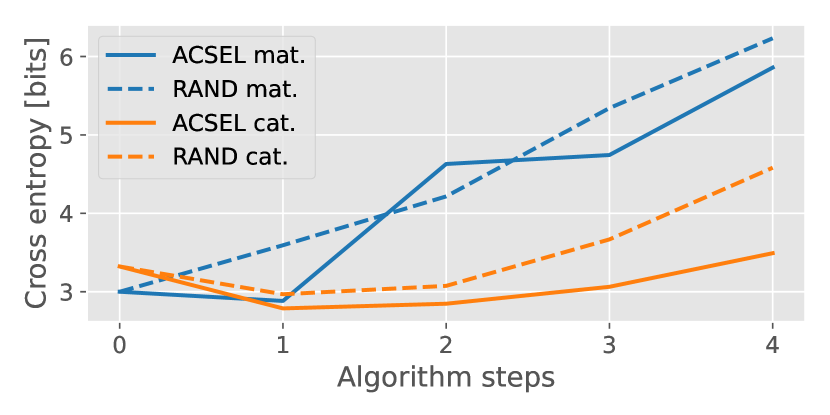
Figure 8: Cross-entropy of the Category and Material nodes – Optimizing Category, 17 objects, 5 repetitions each. Comparing action selection based on IG (ACSEL) and random action selection (RAND).

V Database of object properties and measurements for robot manipulation

Object datasets related to robot manipulation typically contain object models and visual-based representations like images, point clouds, or meshes (e.g., YCB [12]). Datasets containing physical object properties are an exception (e.g., [17, 18, 19]).

The measurements collected in this work provided the foundation for a database of measurements of object physical properties. These measurements are naturally dependent on the objects manipulated and also highly dependent on the embodiment of the robot (e.g., stiffness measurements on the gripper used and the force/effort feedback)—unlike for images where the camera that recorded the images plays less critical role. To be useful, such a database needs to cover different setups: different robots, grippers, sensors, etc. and their description in the metadata. The structure of the database we created is shown in Fig. 9; it is available at https://cmp.felk.cvut.cz/ipalm/.

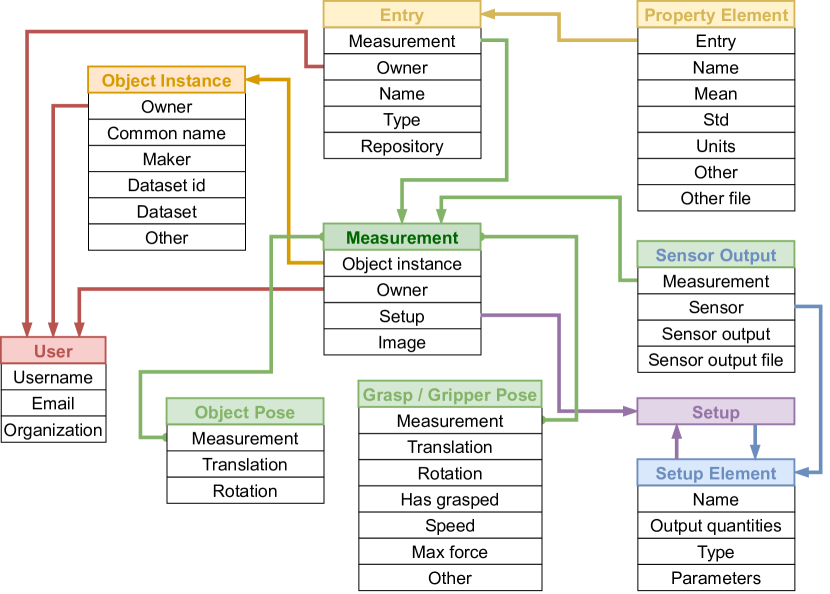
Figure 9: Database of object properties and measurements for robot manipulation – structure.

The database contains all the measurements collected in this work (images, stress/strain curves for stiffness estimation, joint angle and joint torque measurements for mass estimation, and audio responses after poking objects). We have already extended the database with elasticity measurements of the same and different objects using several other grippers (OnRobot RG6, Barrett Hand, QB SoftHand, professional elasticity measurement setup).

Our contribution is aligned with the efforts of others to share robot data across platforms and continents [20]. However, while [20] contains mainly image and joint angle streams, our database is more “strongly embodied”, allowing for storage of multimodal, in particular haptic data. We invite the community to contribute. To make data collection easier in the correct format, we developed a tool that automates this—a Python decorator (Butler), and its source code is available on the database website. One can use this decorator to save data in the desired directory structure and upload them to the database. Using this workflow, we populated the database with more than 24000 measurements for over 60 objects. Ultimately, once enough instances of every object type appear in the database, category-level description grounded in the physical measurements will become available. Generalization across the different devices, which were used to collect the haptic data, remains a fundamental challenge.

VI Conclusion, Discussion, Future Work

We presented an algorithmic framework and experimental setup for learning physical object properties through robot manipulation. Our approach involved exploratory action selection to maximize IG about objects on a table in front of a robot manipulator. At its core, the framework employs a BN model to represent the probabilistic relationships between different object properties. The BN consists of nodes corresponding to various object properties, including categorical properties like Category and Material, as well as continuous properties such as Elasticity, Density, and Volume. We demonstrated the effectiveness of our method through experimental evaluation, showcasing its ability to automatically extract properties such as material composition, mass, volume, and stiffness. The algorithm outperformed random action selection baseline and showed promising results in discovering object properties on a partially adversarial object dataset (with “fake objects” like a stiff sponge). The algorithm can automatically terminate based on the expected IG of the available actions. The code used in this work is available at https://github.com/ctu-vras/actsel. The object database and source code are available at https://cmp.felk.cvut.cz/ipalm/.

Every measurement type in our framework has its own limitations. For example, the Young’s modulus for Elasticity is limited by the resolution of current flowing through the gripper. There is a threshold above which the gripper cannot provide any specific information on the object deformation. This threshold was experimentally found to be $95$ [kPa]. In such cases, the output is binary, providing a half-open set of moduli from the threshold onward. This is an uninformative measurement over all properties above this experimental threshold. This brings a discontinuous change of elasticity belief distribution.

Another source of information degradation is the inference of categorical weights from the continuous GMMs using the EM algorithm. This stems from uncertainties on the numerical level when the belief distribution mean moved too far from the reference labels. Therefore, the only information that the EM algorithm possesses at the location of reference labels is from the far tails of the normal distributions. In the process of normalization to unit-sum probabilities from very small numbers, the numerical errors provide a large variance in results. We tried to tackle this problem using Monte Carlo Markov Chains, more specifically Gibbs’ sampling method, although this has shown to be too computationally expensive to run in real-time.

As part of future work, community engagement and dataset expansion are essential endeavors. By making our dataset and codebase openly accessible, we aim to foster collaboration and knowledge-sharing among researchers in the field of robot learning and manipulation. We encourage contributions from the community to enrich the dataset with diverse object measurements and annotations, facilitating a broader range of research applications and algorithm evaluations. Additionally, active engagement with the community allows us to gather valuable feedback and insights, guiding the evolution of our framework and ensuring its relevance and usefulness in real-world settings. Together, these efforts contribute to the collective advancement of robot learning and manipulation capabilities, ultimately driving innovation and progress in the field.

Another promising avenue for advancement lies in the development of adaptive exploration strategies. By leveraging techniques from reinforcement learning and advanced decision-making algorithms, robots can autonomously learn and refine their exploration policies over time. Adaptive exploration strategies can dynamically adjust the selection of actions based on the robot’s past experience and the current state of uncertainty in object properties. This allows robots to prioritize actions that are more likely to yield informative measurements, leading to more efficient and effective learning of physical object properties.

References

- [1] J. K. Behrens, M. Nazarczuk, K. Stepanova, M. Hoffmann, Y. Demiris, and K. Mikolajczyk, “Embodied reasoning for discovering object properties via manipulation,” in 2021 IEEE International Conference on Robotics and Automation (ICRA). IEEE, 2021, pp. 10 139–10 145.
- [2] A. Dutta, E. Burdet, and M. Kaboli, “Push to know!-visuo-tactile based active object parameter inference with dual differentiable filtering,” in 2023 IEEE/RSJ International Conference on Intelligent Robots and Systems (IROS). IEEE, 2023, pp. 3137–3144.
- [3] T. N. Le, F. Verdoja, F. J. Abu-Dakka, and V. Kyrki, “Probabilistic surface friction estimation based on visual and haptic measurements,” IEEE Robotics and Automation Letters, vol. 6, no. 2, 2021.
- [4] D. Xu, G. E. Loeb, and J. A. Fishel, “Tactile identification of objects using Bayesian exploration,” in 2013 IEEE International Conference on Robotics and Automation. IEEE, 2013, pp. 3056–3061.
- [5] A. Petrovskaya and K. Hsiao, “Active manipulation for perception,” Springer Handbook of Robotics, pp. 1037–1062, 2016.
- [6] V. Chu, I. McMahon, L. Riano, C. G. McDonald, Q. He, J. M. Perez-Tejada, M. Arrigo, N. Fitter, J. C. Nappo, T. Darrell, et al., “Using robotic exploratory procedures to learn the meaning of haptic adjectives,” in 2013 IEEE International Conference on Robotics and Automation. IEEE, 2013, pp. 3048–3055.
- [7] J. A. Fishel and G. E. Loeb, “Bayesian Exploration for Intelligent Identification of Textures,” Frontiers in neurorobotics, vol. 6, p. 4, 2012.
- [8] M. Mahendran, “The Modulus of Elasticity of Steel - Is It 200 GPa?” International Specialty Conference on Cold-Formed Steel Structures, vol. 5, Oct 1996.
- [9] M. Dondi, E. G., M. M., M. C., and C. Mingazzini, “The chemical composition of porcelain stoneware tiles and its influence on microstructure and mechanical properties,” InterCeram: International Ceramic Review, vol. 48, pp. 75–83, 01 1999.
- [10] T. Húlan and I. Štubňa, “Young’s modulus of kaolinite-illite mixtures during firing,” Applied Clay Science, vol. 190, p. 105584, 2020.
- [11] D. C. Giancoli, Physics: Principles with Applications. Pearson, 2014.
- [12] B. Calli, A. Singh, A. Walsman, S. Srinivasa, P. Abbeel, and A. M. Dollar, “The YCB object and Model set: Towards common benchmarks for manipulation research,” in 2015 International Conference on Advanced Robotics (ICAR), 2015, pp. 510–517.
- [13] S. P. Patni, P. Stoudek, H. Chlup, and M. Hoffmann, “Online elasticity estimation and material sorting using standard robot grippers,” arXiv preprint arXiv:2401.08298, 2024.
- [14] M. Dimiccoli, S. Patni, M. Hoffmann, and F. Moreno-Noguer, “Recognizing object surface material from impact sounds for robot manipulation,” in 2022 IEEE/RSJ International Conference on Intelligent Robots and Systems (IROS). IEEE, 2022, pp. 9280–9287.
- [15] Y. Wu, A. Kirillov, F. Massa, W.-Y. Lo, and R. Girshick, “Detectron2,” https://github.com/facebookresearch/detectron2, 2019.
- [16] M. Nazarczuk and K. Mikolajczyk, “SHOP-VRB: A Visual Reasoning Benchmark for Object Perception,” International Conference on Robotics and Automation (ICRA), 2020.
- [17] Z. Chen, K. Yi, Y. Li, M. Ding, A. Torralba, J. B. Tenenbaum, and C. Gan, “Comphy: Compositional physical reasoning of objects and events from videos,” in International Conference on Learning Representations, 2022.
- [18] M. Purri and K. Dana, “Teaching cameras to feel: Estimating tactile physical properties of surfaces from images,” in European Conference on Computer Vision. Springer, 2020, pp. 1–20.
- [19] M. Thosar, C. A. Mueller, G. Jäger, J. Schleiss, N. Pulugu, R. Mallikarjun Chennaboina, S. V. Rao Jeevangekar, A. Birk, M. Pfingsthorn, and S. Zug, “From Multi-Modal Property Dataset to Robot-Centric Conceptual Knowledge About Household Objects,” Frontiers in Robotics and AI, vol. 8, p. 87, 2021.
- [20] Open X-Embodiment Collaboration, A. Padalkar, et al., “Open X-Embodiment: Robotic learning datasets and RT-X models,” https://arxiv.org/abs/2310.08864, 2023.