Sequential Decision Making with Expert Demonstrations under Unobserved Heterogeneity

Abstract

We study the problem of online sequential decision-making given auxiliary demonstrations from experts who made their decisions based on unobserved contextual information. These demonstrations can be viewed as solving related but slightly different tasks than what the learner faces. This setting arises in many application domains, such as self-driving cars, healthcare, and finance, where expert demonstrations are made using contextual information, which is not recorded in the data available to the learning agent. We model the problem as a zero-shot meta-reinforcement learning setting with an unknown task distribution and a Bayesian regret minimization objective, where the unobserved tasks are encoded as parameters with an unknown prior. We propose the Experts-as-Priors algorithm (ExPerior), a non-parametric empirical Bayes approach that utilizes the principle of maximum entropy to establish an informative prior over the learner’s decision-making problem. This prior enables the application of any Bayesian approach for online decision-making, such as posterior sampling. We demonstrate that our strategy surpasses existing behaviour cloning and online algorithms for multi-armed bandits and reinforcement learning, showcasing the utility of our approach in leveraging expert demonstrations across different decision-making setups.

1 Introduction

The allure of reinforcement learning (RL) is evident in its significant successes in various complex decision-making tasks, spanning areas such as game playing (Mnih et al.,, 2013; Silver et al.,, 2016, 2017), robotics (Silver et al.,, 2014; Lillicrap et al.,, 2015), and aligning with human preferences (Ouyang et al.,, 2022). As intelligent and autonomous decision-making systems become more prevalent, the role of RL becomes increasingly central.

However, RL’s considerable sample inefficiency, necessitating millions of training frames for convergence, remains a significant challenge. A notable body of work within RL has been dedicated to integrating expert demonstrations to accelerate the learning process, employing strategies like offline pretraining (Wagenmaker and Pacchiano,, 2023) and the use of combined offline-online datasets (Song et al.,, 2022; Ball et al.,, 2023). While these approaches are theoretically sound and empirically validated (Nair et al.,, 2018; Cabi et al.,, 2019), they typically presume homogeneity between the offline demonstrations and online RL tasks. A vital question arises regarding the effectiveness of these methods when expert demonstrations embody heterogeneous tasks, indistinguishable by the learner.

An important example of such heterogeneity is in situations where experts operate with additional information not available to the learner, a scenario previously explored in imitation learning with unobserved contexts (Briesch et al.,, 2010; Yu et al.,, 2019; Kallus and Zhou,, 2021; Bennett et al.,, 2021). Existing literature either relies the availability of experts to query during training (Choudhury et al.,, 2018; Walsman et al.,, 2022; Shenfeld et al.,, 2023) or focuses on the assumptions that enable imitation learning with unobserved contexts, sidestepping online reward-based interactions (Zhang et al.,, 2020; Swamy et al.,, 2022). Recent contributions by Hao et al., 2023a ; Hao et al., 2023b suggest the utilization of offline expert data for online RL, albeit without accounting for unobserved contextual variations.

Our work addresses the more general challenge of online sequential decision-making given auxiliary offline expert demonstration data with unobserved heterogeneity. We view such demonstrations as solving related yet distinct tasks from those faced by the learner, where differences remain invisible to the learner. For instance, in a personalized education scenario, while a learning agent might access observable characteristics like grades or demographics, it might remain oblivious to factors such as learning styles or family background, which are visible to an expert teacher and can significantly influence teaching methods. A naïve imitation learning algorithm that lacks access to this ”private” information will only learn a single policy for each observed characteristic, leading to sub-optimal decisions. On the other hand, a purely online approach will require extensive trial and error to result in meaningful decisions.

We propose integrating offline expert data with online RL, treating the scenario as a zero-shot meta-reinforcement learning (meta-RL) problem with an unknown distribution over tasks (unobserved factors). Unlike typical meta-RL frameworks where the learner is exposed to multiple tasks during training (different students in our example) to learn the underlying task distribution (Cella et al.,, 2020; Cella and Pontil,, 2021), our approach only leverages offline expert demonstrations to infer this distribution, thus embodying a zero-shot meta-RL paradigm (Mardia et al.,, 2020). In particular, we define a Bayesian regret minimization objective and consider different tasks as parameters under an unknown prior distribution. Using the maximum entropy principle, we derive an informative prior over the decision-making task from the expert data. We then use the learned prior distribution to drive exploration in the online RL task, using approaches like posterior sampling (Osband et al.,, 2013). We call our method Experts-as-Priors or ExPerior for short. See Figure 1 for an illustration of ExPerior in a goal-oriented RL task.

Finally, to rigorously analyze the impact of expert demonstration data under unobserved heterogeneity, we conduct an empirical regret analysis for multi-armed bandits. Our analysis demonstrates that the Bayesian regret incurred by ExPerior is proportional to the entropy of the optimal action under the prior distribution, aligning with the entropy of expert policy if the experts are optimal. Our results suggest the use of entropy of expert demonstrations to evaluate the impact of unobserved factors. In summary, our contributions are:

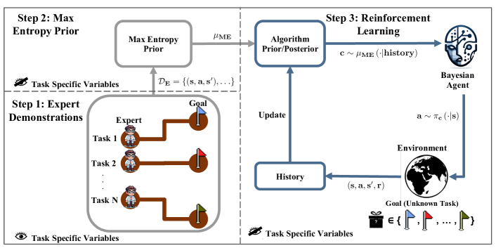
Figure 1: Illustration of ExPerior in a goal-oriented RL task. Step 1 (Offline): The experts demonstrate their policies for related but different tasks (different goals) while observing the goal type. Step 2 (Offline): The expert demonstrations $\mathcal{D}_{\text{E}}$ only contain the trajectories of states and actions taken by experts — goal types are not collected. We form an informative (max-entropy) prior over tasks using $\mathcal{D}_{\text{E}}$. Step 3 (Online): The goal type is unknown but drawn from the same distribution of goals in step 1. The learner uses the derived prior from step 2 and runs posterior sampling.

1. We formulate the use of expert demonstrations in sequential decision-making with unobserved heterogeneity as a zero-shot meta-RL problem, adopting a Bayesian regret minimization perspective that treats unobserved factors as unknown parameters.

2. We propose a nonparametric empirical Bayes approach, guided by the principle of maximum entropy, to derive an informative prior from the expert demonstrations, which in turn aids exploration through Bayesian methods.

3. We empirically showcase the superiority of our algorithm compared to offline, online, and offline-online baselines in multi-armed bandits and RL and provide an empirical regret analysis in multi-armed bandits.

2 Related Work

Our work is an addition to the recent body of reinforcement learning research that leverages offline demonstrations to speed up online learning (Rajeswaran et al.,, 2017; Nair et al.,, 2018, 2020; Wagenmaker and Pacchiano,, 2023; Ball et al.,, 2023). Classic algorithms such as DDPGfD (Vecerik et al.,, 2017) and DQfD (Hester et al.,, 2018) achieve this by combining imitation learning and RL. They modify DDPG (Lillicrap et al.,, 2015) and DQN (Mnih et al.,, 2013) by warm-starting the algorithms’ replay buffers with expert trajectories and ensuring that the offline data never gets overridden by online trajectories. Closely related to our study is the meta-RL literature, which aims to accelerate learning in a given RL task by using prior experience from related tasks (Gupta et al.,, 2018; Nagabandi et al.,, 2018; Beck et al.,, 2023). These papers present model-agnostic meta-learning training objectives to maximize the expected reward from novel tasks as efficiently as possible.

Two unique features distinguish our problem from the settings considered above. First, our setting assumes heterogeneity within the offline demonstration data and with the online RL task that is unobserved to the learner, while the (optimal) experts are privy to that heterogeneity. Second, we assume the learner will only interact with one online task, making our setup similar to zero-shot meta-RL (Mardia et al.,, 2020; Verma et al.,, 2020; Jiang et al.,, 2023).

Most similar to our work is the ExPLORe algorithm (Li et al.,, 2024), which assigns optimistic rewards to the offline data during the online interaction and runs an off-policy algorithm using both online data and labelled offline data as buffers. For our problem setting, the algorithm incentivizes the learner to explore the expert trajectories, leading to faster convergence - we consider this work one of our baselines.

Our methodology utilizes only the state-action trajectory data from expert demonstrations without task-specific information or reward labels. Other similar methods require additional offline information. For example, Nair et al., (2020) assume that the offline data contains the reward labels and use that to pre-train a policy, which is then fine-tuned online. Mendonca et al., (2019) require task labelling for each trajectory and use the offline data to learn a single meta-learner. Similarly, Zhou et al., (2019) and Rakelly et al., (2019) require the task label and reward labels. They then infer the task during online interaction and use the task-specific offline data.

Finally, our methodology builds on posterior sampling (Russo et al.,, 2018). Hao et al., 2023a ; Hao et al., 2023b consider a similar problem using posterior sampling to leverage offline expert demonstration data to improve online RL. However, they assume homogeneity between the expert data and online tasks. In contrast, our setting accounts for heterogeneity.

3 Problem Setup

Decision Model for Unobserved Heterogeneity of Tasks. To account for unobserved heterogeneity, we consider a generalization of finite-horizon Markov Decision Processes (MDPs) with a notion of probabilistic task variables (Hallak et al.,, 2015; Yu et al.,, 2019; Swamy et al.,, 2022). In this setup, the MDP’s underlying model will additionally depend on an unobserved task variable that encapsulates some information about the specific task. For example, consider a personalized education system where educating a specific student corresponds to a task, and the learning agent can observe the students’ characteristics, like their demographic information and grades. However, other factors, such as the student’s learning style (e.g., whether they are visual learners or learn more efficiently during self-study), may not be readily available, even though they are important in determining the optimal teaching style.

To make it concrete, let $\mathcal{C}$ be the set of all unobserved variables that can describe the heterogeneity of potential tasks (e.g., the set of all possible learning styles). A (contextual) MDP $\mathcal{M}=\left(\mathcal{S},\mathcal{A},\mathcal{T},R,H,\rho,\mu^{\star}\right)$ is parameterized by states $\mathcal{S}$, actions $\mathcal{A}$, transition function $\mathcal{T}:\mathcal{S}\times\mathcal{A}\times\mathcal{C}\to\Delta(\mathcal{S})$, reward function $R:\mathcal{S}\times\mathcal{A}\times\mathcal{C}\to\Delta(\operatorname{\mathbb{R}})$, horizon $H>0$, initial state distribution $\rho\in\Delta(\mathcal{S})$, and task distribution $\mu^{\star}$. We assume the transition/reward functions and $\mu^{\star}$ are unknown, and for simplicity, $\rho$ does not depend on the task variable. For each task $c\sim\mu^{\star}$, we consider $T$ episodes, where at the beginning of each episode $t\in[T]$, an initial state $s_{1}\sim\rho$ is sampled. Then, at each timestep $h\in[H]$, the learner chooses an action $a_{h}\in\mathcal{A}$, observes a reward $r_{h}\sim R\left(s_{h},a_{h},c\right)$ and the next state $s_{h+1}\sim\mathcal{T}\left(s_{h},a_{h},c\right)$. Without loss of generality, we assume the states are partitioned by $[H]$ to make the notation invariant to timestep $h$. Let $\Pi$ be the set of all Markovian policies. For a policy function $\pi:\mathcal{S}\to\Delta(\mathcal{A})\in\Pi$ and task variable $c$, we define the value function and Q-function as

$$V_{c}\left(\pi\right)=\operatorname{\mathbb{E}}\left[\sum_{h=1}^{H}r_{h}\ \middle|\ \pi,c\right]\ \text{and}\quad\forall s\in\mathcal{S},a\in\mathcal{A}:\ Q^{\pi}_{c}\left(s,a\right):=\operatorname{\mathbb{E}}\left[\sum_{h^{\prime}=h}^{H}r_{h^{\prime}}\ \middle|\ s_{h}=s,a_{h}=a,\pi,c\right].$$ (1)

Moreover, we define the optimal policy for a task variable $c\in\mathcal{C}$ as $\pi_{c}:=\operatorname*{arg\,max}_{\pi\in\Pi}V_{c}\left(\pi\right)$. Note that since the task variable is unobserved, the learner’s policy will not depend on it. The learner’s goal is to learn history-dependent distributions $p^{1},\ldots,p^{T}\in\Delta(\Pi)$ over Markovian policies to minimize the following notion of regret:

$$\text{Reg}:=\operatorname{\mathbb{E}}_{c\sim\mu^{\star}}\left[\sum_{t=1}^{T}V_{c}(\pi_{c})-\operatorname{\mathbb{E}}_{\pi^{t}\sim p^{t}}\left[V_{c}(\pi^{t})\right]\right].$$ (2)

In the personalized education example, the setup above assumes a fixed distribution $\mu^{\star}$ over the set of learning styles and aims to minimize the expected regret over the whole population of students. Our setup and regret defined in 2 assume the unobserved factors remain fixed during training (the student’s learning style remains unchanged). Making this assumption is practical as the unobserved variables often correspond to less-variant factors (e.g., genetics and lifestyle habits). In general, no learning algorithm can control the regret value if we allow the unobserved factors to change throughout $T$ episodes with no extra structures or access to hidden information. To see this, consider a two-armed bandit with a task value that is drawn with uniform probability from $\mathcal{C}=\{c_{1},c_{2}\}$ and can change at each episode. Now, assume the expected reward of the first arm under $c_{1}$ ($c_{2}$) is one (zero), and it is reversed for the other. It is easy to see that any algorithm that does not have access to $c$ would result in linear regret.

Remark.

Our setup can be formulated as a Bayesian model parameterized by $\mathcal{C}$, and 2 can be seen as the Bayesian regret of the learner. However, the distribution $\mu^{\star}$ here is not the learner’s prior belief about the true model as it is often formulated in Bayesian learning, but a distribution over potential tasks that the learner can encounter. Our setup can be thus seen as a meta-learning or multi-task learning problem. In fact, it is a zero-shot meta-learning problem since we do not assume having access to more than one online task during training — we only learn the prior distribution using the offline data.

Expert Demonstrations. In addition to the online setting described above, we assume the learner has access to an offline dataset of expert demonstrations $\mathcal{D}_{\text{E}}$, where each demonstration $\tau_{\text{E}}=\left(s_{1},a_{1},s_{2},a_{2},\ldots,s_{H},a_{H},s_{H+1}\right)$ refers to an interaction of the expert with a decision-making task during a single episode, containing the actions made by the expert and the resulting states. We assume that the unobserved task-specific variables for $\mathcal{D}_{\text{E}}$ are drawn i.i.d. from distribution $\mu^{\star}$, and the expert had access to such unobserved variables (private information) during their decision-making. Moreover, we assume the expert follows a near-optimal strategy (Hao et al., 2023a, ; Hao et al., 2023b, ).

Assumption 1 (Noisily Rational Expert).

For any $c\in\mathcal{C}$, experts select actions based on a distribution $p_{\text{E}}$ defined as:

$$\forall s\in\mathcal{S},a\in\mathcal{A}:\ p_{\text{E}}\left(a\ \middle|\ s\,;\,c\right)\propto\exp\left\{\beta\cdot Q^{\pi_{c}}_{c}(s,a)\right\},$$ (3)

for some known value of $\beta\in[0,\infty]$. In particular, the expert follows the optimal policy if $\beta\to\infty$.

Note that our setup assumes that the experts do not provide any rationale for their strategy, nor do we have access to rewards in the offline data. This problem can thus be seen as a combination of imitation learning and online learning rather than offline RL.

4 Experts-as-Priors Model for Unobserved Heterogeneity

Our goal is to leverage offline data to help guide the learner through its interaction with the decision-making task. This paper’s main idea is to use expert demonstrations to infer a prior distribution over $\mathcal{C}$ and then to use a Bayesian approach such as posterior sampling (Osband et al.,, 2013) to utilize the inferred prior for a more informative exploration. In particular, if the current task is from the same distribution of tasks in the offline data, we expect that using such priors will lead to faster convergence to optimal trajectories compared to the commonly used non-informative priors. Consider the example of learning a personalized education strategy. Suppose we have gathered offline data on an expert’s teaching strategies for students with similar observed information like grade, age, location, etc. The teacher can observe more fine-grained information about the students that is generally absent from the collected data (their learning style in our example). The space of the optimal strategies for students with similar observed information but different learning styles is often much smaller than the space of all possible strategies. With the inferred prior distribution, the learner needs to focus only on the span of potentially optimal strategies for a new student, allowing for more efficient exploration.

We resort to empirical Bayes and use maximum marginal likelihood estimation (Carlin and Louis,, 2000) to construct a prior distribution from $\mathcal{D}_{\text{E}}$. Given a probability distribution (prior) $\mu$ on $\mathcal{C}$, the marginal likelihood of an expert demonstration $\tau_{\text{E}}=\left(s_{1},a_{1},s_{2},a_{2},\ldots,s_{H},a_{H},s_{H+1}\right)\in\mathcal{D}_{\text{E}}$ is given by

$$\mathrm{P}_{\text{E}}\left(\tau_{\text{E}}\,;\,\mu\right)=\operatorname{\mathbb{E}}_{c\sim\mu}\left[\rho(s_{1})\cdot\prod_{h=1}^{H}p_{\text{E}}\left(a_{h}\ \middle|\ s_{h}\,;\,c\right)\mathcal{T}\left(s_{h+1}\ \middle|\ s_{h},a_{h},c\right)\right].$$ (4)

We aim to find a prior distribution to maximize the log-likelihood of $\mathcal{D}_{\text{E}}$ under the model described in 4. This is equivalent to minimizing the KL divergence between the marginal likelihood $\mathrm{P}_{\text{E}}$ and the empirical distribution of expert demonstrations, which we denote by $\widehat{\mathrm{P}}_{\text{E}}$. In particular, we form the following uncertainty set over the set of plausible priors:

$$\mathcal{P}(\epsilon):=\left\{\mu\,;\,\mathrm{D}_{\mathrm{KL}}\left(\widehat{\mathrm{P}}_{\text{E}}\ \middle\|\ \mathrm{P}_{\text{E}}\left(\cdot\,;\,\mu\right)\right)\leq\epsilon\right\},$$ (5)

where the value of $\epsilon$ can be chosen based on the number of samples so the uncertainty set in 5 contains the true prior with high probability (Mardia et al.,, 2020). However, the set of plausible priors does not uniquely identify the appropriate prior. In fact, even for $\epsilon=0$, $\mathcal{P}(\epsilon)$ can have infinite plausible priors. To solve this ill-posed problem, we employ the principle of maximum entropy to choose the least informative prior that is compatible with expert data.

Definition 1 (Max-Entropy Expert Prior).

Let $\mu_{0}$ be a non-informative prior on $\mathcal{C}$ (e.g., a uniform distribution). Given some $\epsilon>0$, we define the maximum entropy expert prior $\mu_{\text{ME}}$ as the solution to the following optimization problem:

$$\mu_{\text{ME}}=\operatorname*{arg\,min}_{\mu}\ \mathrm{D}_{\mathrm{KL}}\left(\mu\ \middle\|\ \mu_{0}\right)\quad\text{s.t.}\quad\mu\in\mathcal{P}(\epsilon).$$ (6)

Note that the set of plausible priors $\mathcal{P}(\epsilon)$ is a convex set, and therefore, 6 is a convex optimization problem. We can derive the solution to problem 6 using Fenchel’s duality theorem (Rockafellar,, 1997; Dudík et al.,, 2007):

Proposition 1 (Max-Entropy Expert Prior).

Let $N=|\mathcal{D}_{\text{E}}|$ be the number of demonstrations in $\mathcal{D}_{\text{E}}$. For each $c\in\mathcal{C}$ and demonstration $\tau_{\text{E}}=\left(s_{1},a_{1},s_{2},a_{2},\ldots,s_{H},a_{H},s_{H+1}\right)\in\mathcal{D}_{\text{E}}$, define $m_{\tau_{\text{E}}}(c)$ as the (partial) likelihood of $\tau_{\text{E}}$ under $c$:

$$m_{\tau_{\text{E}}}(c)=\prod_{h=1}^{H}p_{\text{E}}\left(a_{h}\ \middle|\ s_{h}\,;\,c\right)\mathcal{T}\left(s_{h+1}\ \middle|\ s_{h},a_{h},c\right).$$ (7)

Denote $\boldsymbol{{\mathrm{m}}}(c)\in\operatorname{\mathbb{R}}^{N}$ as the vector with elements $m_{\tau_{\text{E}}}(c)$ for $\tau_{\text{E}}\in\mathcal{D}_{\text{E}}$. Moreover, let $\lambda^{\star}\in\operatorname{\mathbb{R}}^{\geq 0}$ be the optimal solution to the Lagrange dual problem of 6. Then, the solution to optimization 6 is as follows:

$$\mu_{\text{ME}}(c)=\lim_{n\to\infty}\frac{\exp\left\{\boldsymbol{{\mathrm{m}}}(c)^{\top}\boldsymbol{{\mathrm{\alpha}}}_{n}\right\}}{\operatorname{\mathbb{E}}_{c\sim\mu_{0}}\left[\exp\left\{\boldsymbol{{\mathrm{m}}}(c)^{\top}\boldsymbol{{\mathrm{\alpha}}}_{n}\right\}\right]},$$ (8)

where $\{\boldsymbol{{\mathrm{\alpha}}}_{n}\}_{n=1}^{\infty}$ is a sequence converging to the following supremum:

$$\sup_{{\boldsymbol{{\mathrm{\alpha}}}\in\operatorname{\mathbb{R}}^{N}}} -\log\operatorname{\mathbb{E}}_{c\sim\mu_{0}}\left[\exp\left\{\boldsymbol{{\mathrm{m}}}(c)^{\top}\boldsymbol{{\mathrm{\alpha}}}\right\}\right]+\frac{\lambda^{\star}}{N}\sum_{i=1}^{N}\log\left(\frac{N\cdot\alpha_{i}}{\lambda^{\star}}\right).$$ (9)

The proof is provided in section A.3. Note that, instead of solving for $\lambda^{\star}$, we set it as a hyperparameter and then solve 9. Even though Proposition 1 requires the correct form of Q-functions (and transition functions) for different values of $c$, we will see in the following sections that we can parameterize the Q-functions and treat those parameters as a proxy for the unobserved factors. Once such prior is derived, we can employ any Bayesian approach for the decision-making task. We finish this section by providing a pseudo-algorithm (Algorithm 1) that uses posterior sampling (Osband et al.,, 2013) as one example. The following sections will detail the algorithm for bandits and MDPs.

Algorithm 1 Max-Entropy Posterior Sampling (ExPerior)

1:  Input: Expert demonstrations $\mathcal{D}_{\text{E}}$, Reference distribution $\mu_{0}$, $\lambda^{\star}\geq 0$, and unknown task $c\sim\mu^{\star}$.

2:  $\mu_{\text{ME}}\leftarrow\textsc{MaxEntropyExpertPrior}(\mu_{0},\mathcal{D}_{\text{E}},\lambda^{\star})$

3:  $\textit{history}\leftarrow\{\}$

4:  for episode $t\leftarrow 1,2,\ldots$ do

5:     sample $c_{t}\sim\mu_{\text{ME}}\left(\cdot\ \middle|\ \textit{history}\right)$ // posterior sampling

6:     for timestep $h\leftarrow 1,2,\ldots,H$ do

7:        take action $a^{t}_{h}\sim\pi_{c_{t}}\left(\cdot\ \middle|\ s_{h}\right)$

8:        observe $r^{t}_{h}\sim R(s^{t}_{h},a^{t}_{h},c),\ s^{t}_{h+1}\sim\mathcal{T}\left(s^{t}_{h},a^{t}_{h},c\right)$ and append $(a_{h}^{t},r_{h}^{t},s_{h+1}^{t})$ to history

9:     end for

10:  end for

5 Learning in Bandits

$K$-armed Bandits. To instantiate Algorithm 1 for $K$-armed bandits, note that $\mathcal{S}=\emptyset$, $H=1$, and $\mathcal{A}=\{1,\ldots,K\}$. In this case, each expert demonstration $\tau_{\text{E}}=a$ will be the pulled arm by the expert for a particular bandit and the likelihood function 7 can be simplified as

$$m_{\tau_{\text{E}}}(c)=p_{\text{E}}\left(a\,;\,c\right).$$ (10)

Since the likelihood function 10 only depends on the task variable $c$ through the expert policy $p_{\text{E}}$, and since $p_{\text{E}}$ only depends on $c$ through the mean reward function (Assumption 1), we can consider the set of mean reward functions as a proxy for the unobserved task variables $\mathcal{C}$. For example, in a Bernoulli $K$-armed bandit setting, we can define

$$\mathcal{C}_{\text{Ber}}=\left\{a\mapsto\left\langle\boldsymbol{{\mathrm{e}}}_{a},\boldsymbol{{\mathrm{\theta}}}\right\rangle\,;\,\boldsymbol{{\mathrm{\theta}}}\in[0,1]^{K}\right\}.$$ (11)

Stochastic Contextual Bandits. In stochastic contextual bandits, the state space $\mathcal{S}$ is the set of contexts and $H=1$. Therefore, the likelihood function 7 for a demonstration $\tau_{\text{E}}=(s,a)$ will be

$$m_{\tau_{\text{E}}}(c)=p_{\text{E}}\left(a\ \middle|\ s\,;\,c\right).$$ (12)

Like $K$-armed bandits, the likelihood function 12 only depends on $c$ through the expert policy. Therefore, we can similarly define the set of mean reward functions as the proxy for the unobserved task variables. For instance, we can consider the task parameters for linear contextual bandits as

$$\mathcal{C}_{\text{Lin}}=\left\{(s,a)\mapsto\left\langle\phi\left(s,a\right),\boldsymbol{{\mathrm{\theta}}}\right\rangle\,;\,\boldsymbol{{\mathrm{\theta}}}\in\operatorname{\mathbb{R}}^{d}\right\},$$ (13)

for some known feature function $\phi:\mathcal{S}\times\mathcal{A}\to\operatorname{\mathbb{R}}^{d}$.

Posterior Sampling. With such parameterizations of $\mathcal{C}$ in 11 and 13, we can use Proposition 1 to derive the maximum entropy prior distribution over the task parameters. However, since the derived prior is not a conjugate prior for standard likelihood functions, we cannot sample from the exact posterior in Algorithm 1. Instead, we resort to approximate posterior sampling via stochastic gradient Langevin dynamics (SGLD) (Welling and Teh,, 2011).

In the rest of this section, we aim to evaluate our approach compared to other baselines, including online methods that do not use expert data and offline behaviour cloning. Moreover, we provide an empirical regret analysis for ExPerior based on the informativeness of expert data, number of actions, and number of training episodes.

5.1 Experiments

We consider $K$-armed Bernoulli bandits for our experimental setup. We evaluate the learning algorithms in terms of the Bayesian regret defined in 2 over multiple task distributions $\mu^{\star}$. In particular, we consider $N_{\mu^{\star}}=256$ different beta distributions, where their parameters are randomly sampled from a uniform distribution in $[0,4]$. To estimate the Bayesian regret, we sample $N_{\text{task}}=128$ bandit tasks from each task distribution and calculate the average regret. Moreover, we use $N_{\text{E}}=500$ optimal expert demonstrations for each task distribution in our experiments ($\beta=\infty$).

Baselines. We compare ExPerior to the following baselines:

• Behaviour cloning (BC) learns a policy by minimizing the cross-entropy loss between the expert demonstrations and the agent’s policy solely based on offline data.

• Naïve Thompson sampling (Naïve-TS) chooses the action with the highest sampled mean from a posterior distribution under an uninformative prior. We use SGLD for approximate posterior sampling for a fair comparison.

• Naïve upper confidence bound (Naïve-UCB) algorithm that selects the action with the highest upper confidence bound. Both Naïve-TS and Naïve-UCB ignore expert demonstrations.

• UCB-ExPLORe, a variant of the algorithm proposed by Li et al., (2024) tailored to bandits. It labels the expert data with optimistic rewards and then uses it alongside online data to compute the upper confidence bounds for exploration.

• Oracle-TS that performs exact Thompson sampling having access to the true task distribution $\mu^{\star}$.

Comparison to baselines. Figure 2 demonstrates the average Bayesian regret for various task distributions over $T=1500$ episodes with $K=10$ arms. To better understand the effect of expert data, we categorize the task distributions by the entropy of their optimal actions into low entropy (less than 0.8), high entropy (greater than 1.6), and medium entropy. Oracle-TS outperforms other baselines, yet the performance of ExPerior is the closest to it. We hypothesize that the performance difference between Oracle-TS and ExPerior is primarily due to the use of SGLD for approximate posterior sampling since the former performs exact Thompson sampling. Moreover, the pure online algorithms Naïve-TS and Naïve-UCB, which disregard expert data, display similar performance across different entropy levels, contrasting with other algorithms that show significantly reduced regret in low-entropy contexts. This underlines the impact of expert data in settings where the unobserved confounding has less effect on the optimal actions. Specifically, in the extreme case of no task heterogeneity, BC is anticipated to yield optimal performance. Additionally, Naïve-UCB surpasses UCB-ExPLORe in medium and high entropy settings, possibly due to the over-optimism of the reward labelling in Li et al., (2024), which can hurt the performance when the expert demonstrations are uninformative.

Figure 2: The Bayesian regret of ExPerior and baselines for $K$-armed Bernoulli bandits ($K=10$). We consider three categories of task distributions based on the entropy of the optimal action. ExPerior is the closest to Oracle-TS.

Empirical regret analysis for Experts-as-Priors. We examine how the quality of expert demonstrations affects the Bayesian regret achieved by Algorithm 1. Settings with highly informative demonstrations, where unobserved factors minimally affect the optimal action, should exhibit near-zero regret since there is no diversity in the tasks, and the expert demonstrations only include optimal trajectories for the task at hand. Conversely, in scenarios where unobserved factors significantly influence the optimal actions, we anticipate the regret to align with standard online regret bounds, similar to the outcomes of Thompson sampling with a non-informative prior. To empirically assess this, we conducted trials with ExPerior and Oracle-TS across various numbers of arms, $K\in[2,10]$, over $T=1500$ episodes, calculating the mean and standard deviation of Bayesian regret across $N_{{\mu^{\star}}}=256$ distinct task distributions. As depicted in Figure 3 (a), both ExPerior and Oracle-TS yield sub-linear regret relative to $K$ and $T$, comparable to the established Bayesian regret bound of $\mathcal{O}(\sqrt{KT})$ for Thompson sampling. However, the middle panel indicates that the Bayesian regret of ExPerior is proportional to the entropy of the optimal action, having an almost linear relationship. This observation seems to be in contrast with the standard Bayesian regret bounds for Thompson sampling under correct prior that have shown a sublinear relationship of $\mathcal{O}\left(\sqrt{\mathrm{\text{Ent}}(\pi_{c})}\right)$, where $\mathrm{\text{Ent}}(\pi_{c})$ denotes the entropy of the optimal action under $\mu^{\star}$ (Russo and Van Roy,, 2016). We leave the theoretical regret analysis for ExPerior for future work.

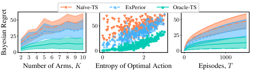
Figure 3: Empirical analysis of ExPerior’s Bayesian regret in Bernoulli bandits based on the (left) number of arms, (middle) entropy of the optimal action, and (right) number of episodes.

6 Learning in MDPs

For MDPs, instead of parameterizing the mean reward functions as done in bandits, we parameterize the optimal Q-functions (e.g., using a deep Q-network) and treat those parameters as a proxy for the unobserved task variables $\mathcal{C}$:

$$\mathcal{C}_{\text{MDP}}:=\left\{(s,a)\mapsto Q\left(s,a\,;\,\boldsymbol{{\mathrm{\theta}}}\right)\,;\,\boldsymbol{{\mathrm{\theta}}}\in\boldsymbol{{\mathrm{\Theta}}}\right\},$$ (14)

where $\boldsymbol{{\mathrm{\Theta}}}$ is the set of parameters for a deep Q-network. The following proposition (proved in section A.4) provides a closed-form expression for the log-pdf posterior of those parameters under the maximum entropy expert prior:

Proposition 2 (Max-Entropy Expert Posterior for MDPs).

Consider a contextual MDP $\mathcal{M}=\left(\mathcal{S},\mathcal{A},\mathcal{T},R,H,\rho,\mu^{\star}\right)$. Assume the transition function $\mathcal{T}$ does not depend on the task variables. Moreover, assume the reward distribution is Gaussian with unit variance and Assumption 1 holds. Then, the log-pdf posterior function under the maximum entropy prior is given as:

$$\begin{split}\forall\boldsymbol{{\mathrm{\theta}}}\in\boldsymbol{{\mathrm{\Theta}}}:\quad\log\mu_{\text{ME}}\left(\boldsymbol{{\mathrm{\theta}}}\ \middle|\ \mathcal{H}_{T}\right)=&-\sum_{t=1}^{T}\sum_{h=1}^{H}\frac{1}{2}\left(r_{h}^{t}+\max_{a^{\prime}\in\mathcal{A}}\operatorname{\mathbb{E}}_{s^{\prime}}\left[Q\left(s^{\prime},a^{\prime}\,;\,\boldsymbol{{\mathrm{\theta}}}\right)\right]-Q\left(s^{t}_{h},a^{t}_{h}\,;\,\boldsymbol{{\mathrm{\theta}}}\right)\right)^{2}\\ &+\sum_{\tau\in\mathcal{D}_{\text{E}}}\alpha^{\star}_{\tau}\cdot\prod_{(s,a)\in\tau}\frac{\exp\left\{\beta\cdot Q\left(s,a\,;\,\boldsymbol{{\mathrm{\theta}}}\right)\right\}}{\sum_{a^{\prime}\in\mathcal{A}}\exp\left\{\beta\cdot Q\left(s,a^{\prime}\,;\,\boldsymbol{{\mathrm{\theta}}}\right)\right\}}+\text{constant in }\boldsymbol{{\mathrm{\theta}}},\end{split}$$ (15)

where $\mathcal{H}_{T}=\left\{\left(\left(s^{t}_{h},a^{t}_{h},r^{t}_{h},s^{t}_{h+1}\right)_{h=1}^{H}\right)_{t=1}^{T}\right\}$ is the history of online interactions, $\mathcal{D}_{\text{E}}$ is the expert demonstration data, $\beta$ is the competence level of the expert in Assumption 1, and $\{\alpha^{\star}_{\tau}\}_{\tau\in\mathcal{D}_{\text{E}}}$ are derived from Proposition 1.

Proposition 2 assumes that the transition function $\mathcal{T}$ does not depend on the task variable for simplicity. We leave the general case for future work. Note that the second term of the posterior is simply the log-pdf of the max-entropy prior.

Posterior Sampling. The log-posterior derived from Proposition 2 can then be used as the loss function for the Deep Q-Network (DQN) algorithm with Langevin Monte Carlo (Dwaracherla and Van Roy,, 2020; Ishfaq et al.,, 2024) as the counterpart for Thompson sampling with SGLD discussed in section 5. However, as observed by Ishfaq et al., (2024), running Langevin dynamics can lead to highly unstable policies due to the complexity of the optimization landscape in deep Q-networks. Instead of sampling from the posterior distribution, we use a heuristic approach by combining the max-entropy expert prior distribution with bootstrapped DQNs (Osband et al.,, 2016).

Max-Entropy Bootstrapped DQN. The original method of Bootstrapped DQNs utilizes an ensemble of randomly initialized Q-networks. It samples a Q-network uniformly at each episode and uses it to collect data. Then, each Q-network is trained using the temporal difference loss (the first term in 15) on parts of or possibly the entire collected data. This method and its subsequent iterations (Osband et al.,, 2018; Osband et al., 2019b, ; Osband et al.,, 2023) achieve deep exploration by ensuring diversity among the learned Q-networks. To utilize the expert data, we initialize the Q-functions in the ensemble with parameters sampled from the max-entropy expert prior. To sample the parameters, we apply SGLD on the log-pdf of the max-entropy prior derived in the second term of 15.

6.1 Experiments

One of the challenges in RL is the sparsity of the reward feedback, where the learning agent needs to explore the environment deeply to observe rewarding states. Utilizing expert demonstrations can significantly enhance the efficiency of deep exploration. For this reason, we focus on the ”Deep Sea” in our experiments, a sparse-reward tabular RL environment proposed by Osband et al., 2019b to assess deep exploration for different RL methods. The environment is an $M\times M$ grid, where the agent starts at the top-left corner of the map, and at each time step, it chooses an action from $\mathcal{A}=\left\{\texttt{left},\texttt{right}\right\}$ to move to the left or right column, while going down by one row. In the original version of Deep Sea, the goal is always on the bottom-right corner of the map. We introduce unobserved task variables by defining a distribution over the goal columns while keeping the goal row the same. We consider four types of goal distributions where the goal is situated at (1) the bottom-right corner of the grid, (2) uniformly at the bottom of any of the right-most $\frac{M}{4}$ columns, (3) uniformly at the bottom of any of the right-most $\frac{M}{2}$ columns, and (4) uniformly at the bottom of any of the $M$ columns. We choose $M=30$ and generate $N=1000$ samples from the optimal policies to use as the offline expert demonstrations.

Baselines. We compare ExPerior to the following baselines. (1) ExPLORe, proposed by Li et al., (2024) to accelerate off-policy reinforcement learning using unlabeled prior data. In this method, the offline demonstrations are assigned optimistic reward labels generated using the online data with regular updates. This information is then combined with the buffer data to perform off-policy learning. (2) Naïve Boot-DQN, which is the original implementation of Bootstrapped DQN with randomly initialized Q-networks (Osband et al.,, 2016). The latter baseline is purely online.

Results. Figure 4 demonstrates the average reward per episode achieved by the baselines for $T=2000$ episodes. For each goal distribution, we run the baselines with $30$ different seeds and take the average to estimate the expected reward. ExPerior outperforms the baselines in all instances. However, the gap between ExPerior and the fully online Naïve Boot-DQN, which measures the effect of using the expert data, decreases as we go from the low-entropy setting (upper left) to the high-entropy task distribution (bottom right). This observation is consistent with the empirical and theoretical results discussed in section 5 and confirms our expectation that the expert demonstrations may not be helpful under strong unobserved confounding (strong task heterogeneity). Moreover, we note that the ExPLORe baseline substantially underperforms, even compared to the fully online Naïve Boot-DQN (except for the first task distribution with zero-entropy). This is potentially because ExPLORe uses actor-critic methods as its backbone model, which are shown to struggle with deep exploration (Osband et al., 2019a, ).

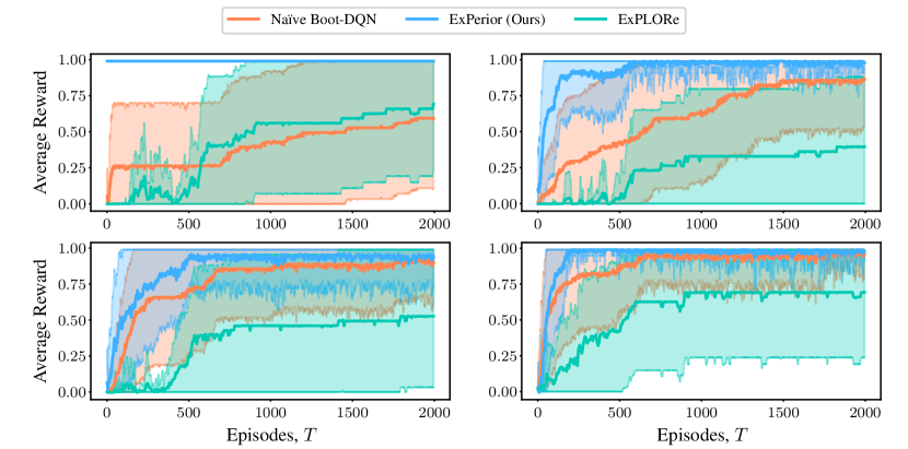
Figure 4: The average reward per episode in terms of the number of episodes in ”Deep Sea.” where the goal is located at (upper left) the right column, (upper right) uniformly at the right-most quarter of the columns, (lower left) uniformly at the right-most half of the columns, and (lower right) uniformly at random over all the columns. ExPerior outperforms the baselines in all instances.

7 Conclusion

This work introduced the Experts-as-Priors (ExPerior) framework, a novel empirical Bayes approach, to address the problem of sequential decision-making using expert demonstrations with unobserved heterogeneity. We grounded our methodology in the maximum entropy principle to infer a prior distribution from expert data that guides the learning process in both bandit settings and Markov Decision Processes (MDPs). Our experimental evaluations demonstrate that ExPerior effectively leverages the expert demonstrations to enhance learning efficiency under unobserved confounding without knowing the confounding level. Specifically, in multi-armed bandits, we illustrated through empirical analysis that the Bayesian regret incurred by ExPerior is proportional to the entropy of the optimal action, highlighting its capacity to adapt based on the informativeness of the expert data. Furthermore, in reinforcement learning, ExPerior showcased its superiority by achieving faster convergence towards optimal policies, as evidenced in the ”Deep Sea” experiments. This performance advantage underscores the utility of our approach in contexts where the learner faces uncertainty and variability in task parameters, a common challenge in real-world applications from autonomous driving to personalized learning environments.

Our work contributes to the understanding of leveraging expert demonstrations under unobserved heterogeneity and offers a practical framework that can be readily applied to a broad spectrum of decision-making tasks. We provide a principled way to incorporate the wealth of information contained in expert behaviours, thus opening new avenues for research in meta-reinforcement learning. Future directions include extending our approach to more complex environments and further investigating our algorithm’s theoretical properties, particularly in regret bounds. By continuing to bridge the gap between offline expert knowledge and online learning processes, we aim to pave the way for more robust, efficient, and adaptable decision-making systems.

Appendix A Proofs

A.1 Notation

We assume $\mathcal{C}$ is a measurable set with an appropriate $\sigma$-algebra and there exists a probability measure $\mu_{0}$ on $\mathcal{C}$. We denote $L^{p}(\mathcal{C},\mu_{0})$ as the space of all measurable functions $f:\mathcal{C}\to\operatorname{\mathbb{R}}$ such that $\|f\|_{p}=\left(\int_{\mathcal{C}}|f|^{p}\mathop{}\!\mathrm{d}\mu_{0}\right)^{1/p}<\infty$. Moreover, we define $L^{\infty}(\mathcal{C},\mu_{0})$ as the space of all essentially bounded measurable functions from $\mathcal{C}$ to $\operatorname{\mathbb{R}}$. Unless stated otherwise, we assume the probability measures are absolutely continuous w.r.t. $\mu_{0}$, and their density functions are in $L^{1}(\mathcal{C},\mu_{0})$. We may abuse the notation and use the same symbol for a probability measure and its Radon–Nikodym derivative w.r.t. $\mu_{0}$. Finally, we use $\operatorname{\mathbb{E}}\left[\cdot\right]$ to denote expectation under the probability measure $\mu_{0}$.

A.2 Useful Lemmas

Here, we state and prove a set of results that will be useful for the rest of this section. The first one is Fenchel’s duality theorem:

Lemma 3 (Fenchel’s Duality (Borwein and Zhu,, 2004)).

Let $X$ and $Y$ be Banach spaces, let $f:X\to\operatorname{\mathbb{R}}\ \cup\ \{+\infty\}$ and $g:Y\to\operatorname{\mathbb{R}}\ \cup\ \{+\infty\}$ be convex functions and let $A:X\to Y$ be a bounded linear map. Define the primal and dual values $p,d\in[-\infty,+\infty]$ by the Fenchel problems

$$p=\inf_{x\in X}f(x)+g(Ax)$$ (16)

$$d=\sup_{y^{*}\in Y^{*}}-f^{*}(A^{*}y^{*})-g^{*}(-y^{*}),$$ (17)

where $f^{*}$ and $g^{*}$ are the Fenchel conjugates of $f$ and $g$ defined as $f^{*}(x^{*})=\sup_{x\in X}\left\langle x^{*},x\right\rangle-f(x)$ (similarly for $g$), $X^{*}$ is the dual space of $X$ and $\left\langle\cdot,\cdot\right\rangle$ is its duality pairing, and $A^{*}:Y^{\star}\to X^{\star}$ is the adjoint operator of $A$, i.e., $\left\langle A^{*}y^{*},x\right\rangle=\left\langle y^{*},Ax\right\rangle$. Suppose $A\ \mathrm{\text{dom}}(f)\cap\mathrm{\text{cont}}(g)\neq\emptyset$, where $\mathrm{\text{dom}}(f):=\left\{x\in X\,;\,f(x)<\infty\right\}$ and $\mathrm{\text{cont}}(g)$ are the continuous points of $g$. Then, strong duality holds, i.e., $p=d$.

Proof.

See the proof of Theorem 4.4.3 in Borwein and Zhu, (2004). ∎

We can use Fenchel’s duality to solve generalized maximum entropy problems. In particular, we prove a generalization of Theorem 2 in Dudík et al., (2007) for density functions in $L^{1}(\mathcal{C},\mu_{0})$:

Lemma 4.

For any function $\mu\in L^{1}(\mathcal{C},\mu_{0})$, define the extended KL divergence as

$$\psi(\mu):=\begin{cases}\mathrm{D}_{\mathrm{KL}}\left(\mu\ \middle\|\ \mu_{0}\right)&\text{ If }\|\mu\|_{1}=1,\\ +\infty&\text{ o.w. }\end{cases}$$ (18)

Moreover, assume a set of bounded feature functions $m_{1},m_{2},\ldots,m_{N}:\mathcal{C}\to\operatorname{\mathbb{R}}$ is given and denote $\boldsymbol{{\mathrm{m}}}$ as the vector of all $N$ features. Consider the linear function $A_{\boldsymbol{{\mathrm{m}}}}:L^{1}(\mathcal{C},\mu_{0})\to\operatorname{\mathbb{R}}^{N}$ defined as

$$\forall\mu\in L^{1}(\mathcal{C},\mu_{0}):\;A_{\boldsymbol{{\mathrm{m}}}}(\mu):=\left(\operatorname{\mathbb{E}}\left[m_{1}\cdot\mu\right],\operatorname{\mathbb{E}}\left[m_{2}\cdot\mu\right],\ldots,\operatorname{\mathbb{E}}\left[m_{N}\cdot\mu\right]\right).$$ (19)

We define the generalized maximum entropy problem as the following:

$$\inf_{\mu\in L^{1}(\mathcal{C},\mu_{0})}\psi(\mu)+\zeta\left(A_{\boldsymbol{{\mathrm{m}}}}(\mu)\right),$$ (20)

for an arbitrary closed proper convex function $\zeta:\operatorname{\mathbb{R}}^{N}\to\operatorname{\mathbb{R}}$. Then the following holds:

1. The dual optimization of 20 is given by

   $$\sup_{\boldsymbol{{\mathrm{\alpha}}}\in\operatorname{\mathbb{R}}^{N}}-\log\operatorname{\mathbb{E}}\left[\exp\left\{\boldsymbol{{\mathrm{m}}}^{\top}\boldsymbol{{\mathrm{\alpha}}}\right\}\right]-\zeta^{*}\left(-\boldsymbol{{\mathrm{\alpha}}}\right),$$ (21)

   where $\zeta^{\star}$ is the convex conjugate function of $\zeta$.

2. Denote $\boldsymbol{{\mathrm{\alpha}}}^{1},\boldsymbol{{\mathrm{\alpha}}}^{2},\ldots$ as a sequence in $\operatorname{\mathbb{R}}^{N}$ converging to supremum 21, and define the following Gibbs density functions

   $$\mu^{\boldsymbol{{\mathrm{\alpha}}}}_{\mathrm{\text{Gibbs}}}\left(c\right):=\frac{\exp\left\{\boldsymbol{{\mathrm{m}}}(c)^{\top}\boldsymbol{{\mathrm{\alpha}}}\right\}}{\operatorname{\mathbb{E}}\left[\exp\left\{\boldsymbol{{\mathrm{m}}}^{\top}\boldsymbol{{\mathrm{\alpha}}}\right\}\right]}.$$ (22)

   Then,

   $$\inf_{\mu\in L^{1}(\mathcal{C},\mu_{0})}\psi(\mu)+\zeta\left(A_{\boldsymbol{{\mathrm{m}}}}(\mu)\right)=\lim_{n\to\infty}\psi(\mu^{\boldsymbol{{\mathrm{\alpha}}}^{n}}_{\mathrm{\text{Gibbs}}})+\zeta\left(A_{\boldsymbol{{\mathrm{m}}}}(\mu_{\mathrm{\text{Gibbs}}}^{\boldsymbol{{\mathrm{\alpha}}}^{n}})\right).$$ (23)

Proof.

Part 1: We first derive the convex conjugate of $\psi$. Note that $\left(L^{1}(\mathcal{C},\mu_{0})\right)^{\star}=L^{\infty}(\mathcal{C},\mu_{0})$ with the pairing

$$\forall h\in L^{\infty}(\mathcal{C},\mu_{0}),\ \mu\in L^{1}(\mathcal{C},\mu_{0}):\;\left\langle h,\mu\right\rangle:=\int_{\mathcal{C}}h(c)\cdot\mu(c)\mathop{}\!\mathrm{d}\mu_{0}.$$ (24)

Hence, by Donsker and Varadhan’s variational formula

$$\forall h\in L^{\infty}(\mathcal{C},\mu_{0}):\;\psi^{\star}(h)=\sup_{\mu\in L^{1}(\mathcal{C},\mu_{0})}\left\langle h,\mu\right\rangle-\psi(\mu)=\log\operatorname{\mathbb{E}}\left[\exp\left\{h\right\}\right].$$ (25)

Moreover, the adjoint operator of $A_{\boldsymbol{{\mathrm{m}}}}$ is given by $A^{\star}_{\boldsymbol{{\mathrm{m}}}}:\operatorname{\mathbb{R}}^{N}\to\left(\mathcal{C}\to\operatorname{\mathbb{R}}\right)$:

$$\forall\boldsymbol{{\mathrm{\alpha}}}\in\operatorname{\mathbb{R}}^{N},\ c\in\mathcal{C}:\;A^{\star}_{\boldsymbol{{\mathrm{m}}}}\left(\boldsymbol{{\mathrm{\alpha}}}\right)\left(c\right)=\boldsymbol{{\mathrm{m}}}\left(c\right)^{\top}\boldsymbol{{\mathrm{\alpha}}}.$$ (26)

Using 25 and 26 and Lemma 3 concludes the proof.

Part 2: Denote the primal and dual objective functions by

$$P(\mu):=\psi(\mu)+\zeta\left(A_{\boldsymbol{{\mathrm{m}}}}(\mu)\right),$$ (27)

$$D(\boldsymbol{{\mathrm{\alpha}}}):=-\log\operatorname{\mathbb{E}}\left[\exp\left\{\boldsymbol{{\mathrm{m}}}^{\top}\boldsymbol{{\mathrm{\alpha}}}\right\}\right]-\zeta^{*}\left(-\boldsymbol{{\mathrm{\alpha}}}\right),$$ (28)

and their optimal values as $P^{*}$ and $D^{*}$. For any $\nu\in L^{1}(\mathcal{C},\mu_{0})$, note that

$$\mathrm{D}_{\mathrm{KL}}\left(\nu\ \middle\|\ \mu_{0}\right)-\mathrm{D}_{\mathrm{KL}}\left(\nu\ \middle\|\ \mu_{\mathrm{\text{Gibbs}}}^{\boldsymbol{{\mathrm{\alpha}}}}\right) =\int_{\mathcal{C}}\nu\log\nu\mathop{}\!\mathrm{d}\mu_{0}-\left(\int_{\mathcal{C}}\nu\log\nu\mathop{}\!\mathrm{d}\mu_{0}-\int_{\mathcal{C}}\nu\log\mu_{\mathrm{\text{Gibbs}}}^{\boldsymbol{{\mathrm{\alpha}}}}\mathop{}\!\mathrm{d}\mu_{0}\right)$$ (29)

$$=\int_{\mathcal{C}}\left(\boldsymbol{{\mathrm{m}}}(c)^{\top}\boldsymbol{{\mathrm{\alpha}}}\right)\nu(c)\mathop{}\!\mathrm{d}\mu_{0}-\log\operatorname{\mathbb{E}}\left[\exp\left\{\boldsymbol{{\mathrm{m}}}^{\top}\boldsymbol{{\mathrm{\alpha}}}\right\}\right]$$ (30)

$$=A_{\boldsymbol{{\mathrm{m}}}}(\nu)^{\top}\boldsymbol{{\mathrm{\alpha}}}-\log\operatorname{\mathbb{E}}\left[\exp\left\{\boldsymbol{{\mathrm{m}}}^{\top}\boldsymbol{{\mathrm{\alpha}}}\right\}\right].$$ (31)

Using 31, we can re-write the dual objective function as:

$$\forall\boldsymbol{{\mathrm{\alpha}}}\in\operatorname{\mathbb{R}}^{N},\nu\in L^{1}(\mathcal{C},\mu_{0}):\quad D(\boldsymbol{{\mathrm{\alpha}}}) =-\mathrm{D}_{\mathrm{KL}}\left(\nu\ \middle\|\ \mu_{\mathrm{\text{Gibbs}}}^{\boldsymbol{{\mathrm{\alpha}}}}\right)+\mathrm{D}_{\mathrm{KL}}\left(\nu\ \middle\|\ \mu_{0}\right)-A_{\boldsymbol{{\mathrm{m}}}}(\nu)^{\top}\boldsymbol{{\mathrm{\alpha}}}-\zeta^{\star}(-\boldsymbol{{\mathrm{\alpha}}}).$$ (32)

Moreover, note that

$$-A_{\boldsymbol{{\mathrm{m}}}}(\nu)^{\top}\boldsymbol{{\mathrm{\alpha}}}-\zeta^{\star}(-\boldsymbol{{\mathrm{\alpha}}}) =-A_{\boldsymbol{{\mathrm{m}}}}(\nu)^{\top}\boldsymbol{{\mathrm{\alpha}}}-\left(\sup_{x}\left\langle x,-\alpha\right\rangle-\zeta(x)\right)$$ (33)

$$\leq-A_{\boldsymbol{{\mathrm{m}}}}(\nu)^{\top}\boldsymbol{{\mathrm{\alpha}}}-\Big{(}\left\langle A_{\boldsymbol{{\mathrm{m}}}}(\nu),-\alpha\right\rangle-\zeta(A_{\boldsymbol{{\mathrm{m}}}}(\nu))\Big{)}$$ (34)

$$=\zeta(A_{\boldsymbol{{\mathrm{m}}}}(\nu)).$$ (35)

Combining 32 and 35, we get

$$\forall\boldsymbol{{\mathrm{\alpha}}}\in\operatorname{\mathbb{R}}^{N},\nu\in L^{1}(\mathcal{C},\mu_{0}):\quad D(\boldsymbol{{\mathrm{\alpha}}}) \leq-\mathrm{D}_{\mathrm{KL}}\left(\nu\ \middle\|\ \mu_{\mathrm{\text{Gibbs}}}^{\boldsymbol{{\mathrm{\alpha}}}}\right)+\mathrm{D}_{\mathrm{KL}}\left(\nu\ \middle\|\ \mu_{0}\right)+\zeta(A_{\boldsymbol{{\mathrm{m}}}}(\nu))$$ (36)

$$=-\mathrm{D}_{\mathrm{KL}}\left(\nu\ \middle\|\ \mu_{\mathrm{\text{Gibbs}}}^{\boldsymbol{{\mathrm{\alpha}}}}\right)+P(\nu).$$ (37)

Now, fix an arbitrary $\epsilon>0$, and consider a sequence of $\mu^{1},\mu^{2},\ldots\in L^{1}(\mathcal{C},\mu_{0})$ such that for all $j\in\operatorname{\mathbb{N}}$:

$$P(\mu^{j})-P^{*}<\frac{\epsilon}{2^{j}}.$$ (38)

We can re-write 38 using the fact $P^{*}=D^{*}=\lim_{n\to\infty}D(\boldsymbol{{\mathrm{\alpha}}}^{n})$:

$$\forall j\in\operatorname{\mathbb{N}}:\quad\lim_{n\to\infty}P(\mu^{j})-D(\boldsymbol{{\mathrm{\alpha}}}^{n})<\frac{\epsilon}{2^{j}}$$ (39)

In particular, by setting $\nu=\mu^{j}$ in 37 and combining the result with 39, we get

$$\forall j\in\operatorname{\mathbb{N}}:\quad\lim_{n\to\infty}\mathrm{D}_{\mathrm{KL}}\left(\mu^{j}\ \middle\|\ \mu_{\mathrm{\text{Gibbs}}}^{\boldsymbol{{\mathrm{\alpha}}}^{n}}\right)<\frac{\epsilon}{2^{j}}.$$ (40)

Hence, $\lim_{j\in\infty}\lim_{n\to\infty}\mathrm{D}_{\mathrm{KL}}\left(\mu^{j}\ \middle\|\ \mu_{\mathrm{\text{Gibbs}}}^{\boldsymbol{{\mathrm{\alpha}}}^{n}}\right)=0$. From properties of the KL divergence, it follows that $\lim_{j\to\infty}P(\mu^{j})=\lim_{n\to\infty}P(\mu_{\mathrm{\text{Gibbs}}}^{\boldsymbol{{\mathrm{\alpha}}}^{n}})$, concluding the proof. ∎

A.3 Max-Entropy Prior

Proposition 1.

Let $N=|\mathcal{D}_{\text{E}}|$ be the number of demonstrations in $\mathcal{D}_{\text{E}}$. For each $c\in\mathcal{C}$ and demonstration $\tau_{\text{E}}=\left(s_{1},a_{1},s_{2},a_{2},\ldots,s_{H},a_{H},s_{H+1}\right)\in\mathcal{D}_{\text{E}}$, define $m_{\tau_{\text{E}}}(c)$ as the (partial) likelihood of $\tau_{\text{E}}$ under $c$:

$$m_{\tau_{\text{E}}}(c)=\prod_{h=1}^{H}p_{\text{E}}\left(a_{h}\ \middle|\ s_{h}\,;\,c\right)\mathcal{T}\left(s_{h+1}\ \middle|\ s_{h},a_{h},c\right).$$ (41)

Denote $\boldsymbol{{\mathrm{m}}}(c)\in\operatorname{\mathbb{R}}^{N}$ as the vector with elements $m_{\tau_{\text{E}}}(c)$ for $\tau_{\text{E}}\in\mathcal{D}_{\text{E}}$. Moreover, let $\lambda^{\star}\in\operatorname{\mathbb{R}}^{\geq 0}$ be the optimal solution to the Lagrange dual problem of 6. Then, the solution to optimization 6 is as follows:

$$\mu_{\text{ME}}(c)=\lim_{n\to\infty}\frac{\exp\left\{\boldsymbol{{\mathrm{m}}}(c)^{\top}\boldsymbol{{\mathrm{\alpha}}}_{n}\right\}}{\operatorname{\mathbb{E}}_{c\sim\mu_{0}}\left[\exp\left\{\boldsymbol{{\mathrm{m}}}(c)^{\top}\boldsymbol{{\mathrm{\alpha}}}_{n}\right\}\right]},$$ (42)

where $\{\boldsymbol{{\mathrm{\alpha}}}_{n}\}_{n=1}^{\infty}$ is a sequence converging to the following supremum:

$$\sup_{{\boldsymbol{{\mathrm{\alpha}}}\in\operatorname{\mathbb{R}}^{N}}} -\log\operatorname{\mathbb{E}}_{c\sim\mu_{0}}\left[\exp\left\{\boldsymbol{{\mathrm{m}}}(c)^{\top}\boldsymbol{{\mathrm{\alpha}}}\right\}\right]+\frac{\lambda^{\star}}{N}\sum_{i=1}^{N}\log\left(\frac{N\cdot\alpha_{i}}{\lambda^{\star}}\right).$$ (43)

Proof.

We first simplify the KL-divergence between the empirical distribution of the expert trajectories $\widehat{\mathrm{P}}_{\text{E}}$ and the marginal likelihood $\mathrm{P}_{\text{E}}\left(\cdot\,;\,\mu\right)$:

$$\mathrm{D}_{\mathrm{KL}}\left(\widehat{\mathrm{P}}_{\text{E}}\ \middle\|\ \mathrm{P}_{\text{E}}\left(\cdot\,;\,\mu\right)\right) =\sum_{\tau^{(i)}\in\mathcal{D}_{\text{E}}}\widehat{\mathrm{P}}_{\text{E}}(\tau^{(i)})\log\frac{\widehat{\mathrm{P}}_{\text{E}}(\tau^{(i)})}{\mathrm{P}_{\text{E}}\left(\tau^{(i)}\,;\,\mu\right)}$$ (44)

$$=-\log N-\frac{1}{N}\sum_{\tau^{(i)}\in\mathcal{D}_{\text{E}}}\log{\mathrm{P}_{\text{E}}\left(\tau^{(i)}\,;\,\mu\right)} \widehat{\mathrm{P}}_{\text{E}}(\tau^{(i)})=\frac{1}{N}$$ ()

$$=-\log N-\frac{1}{N}\sum_{\tau^{(i)}\in\mathcal{D}_{\text{E}}}\log\operatorname{\mathbb{E}}\left[m_{\tau^{(i)}}\cdot\mu\right]-\frac{1}{N}\sum_{s_{1}^{(i)}\in\mathcal{D}_{\text{E}}}\log\rho\left(s_{1}^{(i)}\right).$$ By 4 and 41

Using the above equality, we can re-write the definition of uncertainty set $\mathcal{P}(\epsilon)$ in 5 as

$$\mathcal{P}(\epsilon)=\left\{\mu\,;\,-\frac{1}{N}\sum_{\tau\in\mathcal{D}_{\text{E}}}\log\operatorname{\mathbb{E}}\left[m_{\tau}\cdot\mu\right]-\epsilon-\log N-\frac{1}{N}\sum_{s_{1}\in\mathcal{D}_{\text{E}}}\log\rho\left(s_{1}\right)\leq 0\right\}.$$ (45)

Therefore, we can re-write the optimization 6 as

$$\mu_{\text{ME}}= \operatorname*{arg\,min}_{\mu\in L^{1}(\mathcal{C},\mu_{0})}\ \psi(\mu)\quad\text{s.t.}\quad-\frac{1}{N}\sum_{\tau\in\mathcal{D}_{\text{E}}}\log\operatorname{\mathbb{E}}\left[m_{\tau}\cdot\mu\right]-\epsilon-\log N-\frac{1}{N}\sum_{s_{1}\in\mathcal{D}_{\text{E}}}\log\rho\left(s_{1}\right)\leq 0,$$ (46)

where the extended KL divergence $\psi(\mu)$ is defined as:

$$\psi(\mu):=\begin{cases}\mathrm{D}_{\mathrm{KL}}\left(\mu\ \middle\|\ \mu_{0}\right)&\text{ If }\|\mu\|_{1}=1,\\ +\infty&\text{ o.w. }\end{cases}$$ (47)

Note that $\mathcal{P}(\epsilon)$ is a convex set. To see this, consider $\mu_{1},\mu_{2}\in\mathcal{P}(\epsilon)$. Then, for any $0\leq\lambda\leq 1$, we have $\mu=(1-\lambda)\mu_{1}+\lambda\mu_{2}\in\mathcal{P}(\epsilon)$ since $\operatorname{\mathbb{E}}\left[m_{\tau}\cdot\mu\right]$ is linear in $\mu$ and $-\log$ is convex. Moreover, It is easy to see there exists a strictly feasible solution for 46 (e.g., consider the true distribution $\mu^{\star}$ over $\mathcal{C}$). Thus, strong duality holds, and we can form the Lagrangian function as

$$L(\mu,\lambda):=\psi(\mu)+\lambda\left(\frac{1}{N}\sum_{\tau\in\mathcal{D}_{\text{E}}}-\log\operatorname{\mathbb{E}}\left[m_{\tau}\cdot\mu\right]\right)-\lambda\left(\epsilon+\log N+\frac{1}{N}\sum_{s_{1}\in\mathcal{D}_{\text{E}}}\log\rho\left(s_{1}\right)\right).$$ (48)

Given that $\lambda^{\star}\in\operatorname{\mathbb{R}}^{\geq 0}$ is the optimal solution to the Lagrange dual problem, the maximum entropy prior $\mu_{\text{ME}}$ will be the solution to

$$\inf_{\mu\in L^{1}\left(\mathcal{C},\mu_{0}\right)}L(\mu,\lambda^{\star})=\inf_{\mu\in L^{1}\left(\mathcal{C},\mu_{0}\right)}\psi(\mu)+\lambda^{\star}\left(\frac{1}{N}\sum_{\tau\in\mathcal{D}_{\text{E}}}-\log\operatorname{\mathbb{E}}\left[m_{\tau}\cdot\mu\right]\right)+\text{constant in }\mu.$$ (49)

Now, for each $\boldsymbol{{\mathrm{x}}}\in\operatorname{\mathbb{R}}^{N}$, define the convex function $\zeta(\boldsymbol{{\mathrm{x}}}):=\frac{\lambda^{\star}}{N}\left(\sum_{i=1}^{N}-\log x_{i}\right)$. Moreover, for $\mu\in L^{1}(\mathcal{C},\mu_{0})$, define $A_{\boldsymbol{{\mathrm{m}}}}(\mu):=\left(\operatorname{\mathbb{E}}\left[m_{\tau^{(1)}}\cdot\mu\right],\operatorname{\mathbb{E}}\left[m_{\tau^{(2)}}\cdot\mu\right],\ldots,\operatorname{\mathbb{E}}\left[m_{\tau^{(N)}}\cdot\mu\right]\right)$. Then,

$$L(\mu,\lambda^{\star})=\psi(\mu)+\zeta\left(A_{\boldsymbol{{\mathrm{m}}}}(\mu)\right).$$ (50)

Combining 49 and 50, the maximum entropy prior $\mu_{\text{ME}}$ is the solution to

$$\inf_{\mu\in L^{1}\left(\mathcal{C},\mu_{0}\right)}\psi(\mu)+\zeta\left(A_{\boldsymbol{{\mathrm{m}}}}(\mu)\right).$$ (51)

Using Lemma 4 and noting that

$$\zeta^{*}(x^{*})=\frac{\lambda^{\star}}{N}\left(\sum_{i=1}^{N}-1-\log\left(-\frac{N}{\lambda^{\star}}\cdot x^{*}_{i}\right)\right)$$ (52)

concludes the proof. ∎

A.4 Max-Entropy Expert Posterior for MDPs

Proposition 2.

Consider a contextual MDP $\mathcal{M}=\left(\mathcal{S},\mathcal{A},\mathcal{T},R,H,\rho,\mu^{\star}\right)$. Assume the transition function $\mathcal{T}$ does not depend on the task variables. Moreover, assume the reward distribution is Gaussian with unit variance and Assumption 1 holds. Then, the log-pdf posterior function under the maximum entropy prior is given as:

$$\forall\boldsymbol{{\mathrm{\theta}}}\in\boldsymbol{{\mathrm{\Theta}}}:\quad\log\mu_{\text{ME}}\left(\boldsymbol{{\mathrm{\theta}}}\ \middle|\ \mathcal{H}_{T}\right)= -\sum_{t=1}^{T}\sum_{h=1}^{H}\frac{1}{2}\left(r_{h}^{t}+\max_{a^{\prime}\in\mathcal{A}}\operatorname{\mathbb{E}}_{s^{\prime}}\left[Q\left(s^{\prime},a^{\prime}\,;\,\boldsymbol{{\mathrm{\theta}}}\right)\right]-Q\left(s^{t}_{h},a^{t}_{h}\,;\,\boldsymbol{{\mathrm{\theta}}}\right)\right)^{2}$$ (53)

$$+\sum_{\tau\in\mathcal{D}_{\text{E}}}\alpha^{\star}_{\tau}\cdot\prod_{(s,a)\in\tau}\frac{\exp\left\{\beta\cdot Q\left(s,a\,;\,\boldsymbol{{\mathrm{\theta}}}\right)\right\}}{\sum_{a^{\prime}\in\mathcal{A}}\exp\left\{\beta\cdot Q\left(s,a^{\prime}\,;\,\boldsymbol{{\mathrm{\theta}}}\right)\right\}}+\text{constant in }\boldsymbol{{\mathrm{\theta}}},$$ (54)

where $\mathcal{H}_{T}=\left\{\left(\left(s^{t}_{h},a^{t}_{h},r^{t}_{h},s^{t}_{h+1}\right)_{h=1}^{H}\right)_{t=1}^{T}\right\}$ is the history of online interactions, $\mathcal{D}_{\text{E}}$ is the expert demonstration data, $\beta$ is the competence level of the expert in Assumption 1, and $\{\alpha^{\star}_{\tau}\}_{\tau\in\mathcal{D}_{\text{E}}}$ are derived from Proposition 1.

Proof.

Since the transition function is task-independent, the likelihood of an expert trajectory $\tau_{\text{E}}$ can be simplified as:

$$\forall c\in\mathcal{C}:\quad m_{\tau_{\text{E}}}(c)=\prod_{h=1}^{H}p_{\text{E}}\left(a_{h}\ \middle|\ s_{h}\,;\,c\right)\cdot\prod_{h=1}^{H}\mathcal{T}\left(s_{h+1}\ \middle|\ s_{h},a_{h}\right).$$ (55)

The second term in 55 is constant in $c$. This implies that the likelihood function $m_{\tau_{\text{E}}}(c)$ will depend on $c$ only through the expert policy, which itself is a function of optimal Q-functions by Assumption 1. Note that the second term in the definition of $m_{\tau_{\text{E}}}$ can be simply removed since we can re-weight the parameters $\boldsymbol{{\mathrm{\alpha}}}$ in the optimization step 9 of Proposition 1. Hence, assuming the deep Q-network is expressive enough, without loss of generality, we can re-define the likelihood function of an expert trajectory $\tau_{\text{E}}=\left(s_{1},a_{1},s_{2},a_{2},\ldots,s_{H},a_{H},s_{H+1}\right)$ as

$$\forall\boldsymbol{{\mathrm{\theta}}}\in\Theta:\quad m_{\tau_{\text{E}}}(\boldsymbol{{\mathrm{\theta}}})=\prod_{h=1}^{H}\frac{\exp\left\{\beta\cdot Q\left(s_{h},a_{h}\,;\,\boldsymbol{{\mathrm{\theta}}}\right)\right\}}{\sum_{a^{\prime}\in\mathcal{A}}\exp\left\{\beta\cdot Q\left(s_{h},a^{\prime}\,;\,\boldsymbol{{\mathrm{\theta}}}\right)\right\}}.$$ (56)

We can now write the log-pdf of the posterior distribution of $\boldsymbol{{\mathrm{\theta}}}$ given $\mathcal{H}_{T}$:

$$\forall\boldsymbol{{\mathrm{\theta}}}\in\Theta:\quad \log\mu_{\text{ME}}\left(\boldsymbol{{\mathrm{\theta}}}\ \middle|\ \mathcal{H}_{T}\right)$$ (57)

$$\quad=\log\mathrm{P}\left(\mathcal{H}_{T}\ \middle|\ \boldsymbol{{\mathrm{\theta}}}\right)+\log\mu_{\text{ME}}(\boldsymbol{{\mathrm{\theta}}})+\text{constant in }\boldsymbol{{\mathrm{\theta}}}$$ (58)

$$\quad=\sum_{t=1}^{L}\sum_{h=1}^{H}\log\rho\left(s^{t}_{1}\right)+\log R\left(r^{t}_{h}\ \middle|\ s^{t}_{h},a^{t}_{h}\,;\,\boldsymbol{{\mathrm{\theta}}}\right)+\log\mathcal{T}\left(s^{t}_{h+1}\ \middle|\ s^{t}_{h},a^{t}_{h}\right)+\log\mu_{\text{ME}}(\boldsymbol{{\mathrm{\theta}}})+\text{const.}$$ (59)

$$\quad=\sum_{t=1}^{L}\sum_{h=1}^{H}\log R\left(r^{t}_{h}\ \middle|\ s^{t}_{h},a^{t}_{h}\,;\,\boldsymbol{{\mathrm{\theta}}}\right)+\log\mu_{\text{ME}}(\boldsymbol{{\mathrm{\theta}}})+\text{const.},$$ (60)

Now, given the Bellman equations, we can write the mean value of the reward function as

$$\forall s\in\mathcal{S},a\in\mathcal{A}:\quad\operatorname{\mathbb{E}}\left[R\left(s,a\,;\,\boldsymbol{{\mathrm{\theta}}}\right)\right]=Q\left(s,a\,;\,\boldsymbol{{\mathrm{\theta}}}\right)-\max_{a^{\prime}\in\mathcal{A}}\operatorname{\mathbb{E}}_{s^{\prime}}\left[Q\left(s^{\prime},a^{\prime}\,;\,\boldsymbol{{\mathrm{\theta}}}\right)\right]$$ (61)

The reward distribution is Gaussian with unit variance. Therefore,

$$\forall s\in\mathcal{S},a\in\mathcal{A},r\in\operatorname{\mathbb{R}}:\quad R\left(r\ \middle|\ s,a\,;\,\boldsymbol{{\mathrm{\theta}}}\right)=\mathcal{N}\left(Q\left(s,a\,;\,\boldsymbol{{\mathrm{\theta}}}\right)-\max_{a^{\prime}\in\mathcal{A}}\operatorname{\mathbb{E}}_{s^{\prime}}\left[Q\left(s^{\prime},a^{\prime}\,;\,\boldsymbol{{\mathrm{\theta}}}\right)\right],1\right).$$ (62)

Moreover, by Proposition 1, the log-pdf of the maximum entropy expert prior is given as

$$\forall\boldsymbol{{\mathrm{\theta}}}\in\Theta:\quad\log\mu_{\text{ME}}(\boldsymbol{{\mathrm{\theta}}})=\sum_{\tau\in\mathcal{D}_{\text{E}}}\alpha^{\star}_{\tau}\cdot m_{\tau}(\boldsymbol{{\mathrm{\theta}}})=\sum_{\tau\in\mathcal{D}_{\text{E}}}\alpha^{\star}_{\tau}\cdot\prod_{(s,a)\in\tau}\frac{\exp\left\{\beta\cdot Q\left(s,a\,;\,\boldsymbol{{\mathrm{\theta}}}\right)\right\}}{\sum_{a^{\prime}\in\mathcal{A}}\exp\left\{\beta\cdot Q\left(s,a^{\prime}\,;\,\boldsymbol{{\mathrm{\theta}}}\right)\right\}}.$$ (63)

Combining 60, 62, and 63, we conclude the proof. ∎

References

- Ball et al., (2023) Ball, P. J., Smith, L., Kostrikov, I., and Levine, S. (2023). Efficient online reinforcement learning with offline data. arXiv preprint arXiv:2302.02948.
- Beck et al., (2023) Beck, J., Vuorio, R., Liu, E. Z., Xiong, Z., Zintgraf, L., Finn, C., and Whiteson, S. (2023). A survey of meta-reinforcement learning. arXiv preprint arXiv:2301.08028.
- Bennett et al., (2021) Bennett, A., Kallus, N., Li, L., and Mousavi, A. (2021). Off-policy Evaluation in Infinite-Horizon Reinforcement Learning with Latent Confounders. In Proceedings of The 24th International Conference on Artificial Intelligence and Statistics, pages 1999–2007. PMLR. ISSN: 2640-3498.
- Borwein and Zhu, (2004) Borwein, J. M. and Zhu, Q. J. (2004). Techniques of variational analysis.
- Briesch et al., (2010) Briesch, R. A., Chintagunta, P. K., and Matzkin, R. L. (2010). Nonparametric Discrete Choice Models With Unobserved Heterogeneity. Journal of Business & Economic Statistics, 28(2):291–307. Publisher: [American Statistical Association, Taylor & Francis, Ltd.].
- Cabi et al., (2019) Cabi, S., Colmenarejo, S. G., Novikov, A., Konyushkova, K., Reed, S., Jeong, R., Zolna, K., Aytar, Y., Budden, D., Vecerik, M., et al. (2019). Scaling data-driven robotics with reward sketching and batch reinforcement learning. arXiv preprint arXiv:1909.12200.
- Carlin and Louis, (2000) Carlin, B. P. and Louis, T. A. (2000). Empirical bayes: Past, present and future. Journal of the American Statistical Association, 95(452):1286–1289.
- Cella et al., (2020) Cella, L., Lazaric, A., and Pontil, M. (2020). Meta-learning with stochastic linear bandits. In International Conference on Machine Learning, pages 1360–1370. PMLR.
- Cella and Pontil, (2021) Cella, L. and Pontil, M. (2021). Multi-task and meta-learning with sparse linear bandits. In Uncertainty in Artificial Intelligence, pages 1692–1702. PMLR.
- Choudhury et al., (2018) Choudhury, S., Bhardwaj, M., Arora, S., Kapoor, A., Ranade, G., Scherer, S., and Dey, D. (2018). Data-driven planning via imitation learning. The International Journal of Robotics Research, 37(13-14):1632–1672.
- Dudík et al., (2007) Dudík, M., Phillips, S. J., and Schapire, R. E. (2007). Maximum entropy density estimation with generalized regularization and an application to species distribution modeling. Journal of Machine Learning Research.
- Dwaracherla and Van Roy, (2020) Dwaracherla, V. and Van Roy, B. (2020). Langevin dqn. arXiv preprint arXiv:2002.07282.
- Gupta et al., (2018) Gupta, A., Mendonca, R., Liu, Y., Abbeel, P., and Levine, S. (2018). Meta-reinforcement learning of structured exploration strategies. Advances in neural information processing systems, 31.
- Hallak et al., (2015) Hallak, A., Di Castro, D., and Mannor, S. (2015). Contextual markov decision processes. arXiv preprint arXiv:1502.02259.
- (15) Hao, B., Jain, R., Lattimore, T., Van Roy, B., and Wen, Z. (2023a). Leveraging demonstrations to improve online learning: Quality matters. arXiv preprint arXiv:2302.03319.
- (16) Hao, B., Jain, R., Tang, D., and Wen, Z. (2023b). Bridging imitation and online reinforcement learning: An optimistic tale. arXiv preprint arXiv:2303.11369.
- Hester et al., (2018) Hester, T., Vecerik, M., Pietquin, O., Lanctot, M., Schaul, T., Piot, B., Horgan, D., Quan, J., Sendonaris, A., Osband, I., et al. (2018). Deep q-learning from demonstrations. In Proceedings of the AAAI conference on artificial intelligence.
- Ishfaq et al., (2024) Ishfaq, H., Lan, Q., Xu, P., Mahmood, A. R., Precup, D., Anandkumar, A., and Azizzadenesheli, K. (2024). Provable and practical: Efficient exploration in reinforcement learning via langevin monte carlo. In The Twelfth International Conference on Learning Representations.
- Jiang et al., (2023) Jiang, J., Lerman, K., and Ferrara, E. (2023). Zero-shot meta-learning for small-scale data from human subjects. In 2023 IEEE 11th International Conference on Healthcare Informatics (ICHI), pages 311–320. IEEE.
- Kallus and Zhou, (2021) Kallus, N. and Zhou, A. (2021). Minimax-Optimal Policy Learning Under Unobserved Confounding. Management Science, 67(5):2870–2890.
- Li et al., (2024) Li, Q., Zhang, J., Ghosh, D., Zhang, A., and Levine, S. (2024). Accelerating exploration with unlabeled prior data. Advances in Neural Information Processing Systems, 36.
- Lillicrap et al., (2015) Lillicrap, T. P., Hunt, J. J., Pritzel, A., Heess, N., Erez, T., Tassa, Y., Silver, D., and Wierstra, D. (2015). Continuous control with deep reinforcement learning. arXiv preprint arXiv:1509.02971.
- Mardia et al., (2020) Mardia, J., Jiao, J., Tánczos, E., Nowak, R. D., and Weissman, T. (2020). Concentration inequalities for the empirical distribution of discrete distributions: beyond the method of types. Information and Inference: A Journal of the IMA, 9(4):813–850.
- Mendonca et al., (2019) Mendonca, R., Gupta, A., Kralev, R., Abbeel, P., Levine, S., and Finn, C. (2019). Guided meta-policy search. Advances in Neural Information Processing Systems, 32.
- Mnih et al., (2013) Mnih, V., Kavukcuoglu, K., Silver, D., Graves, A., Antonoglou, I., Wierstra, D., and Riedmiller, M. (2013). Playing atari with deep reinforcement learning. arXiv preprint arXiv:1312.5602.
- Nagabandi et al., (2018) Nagabandi, A., Clavera, I., Liu, S., Fearing, R. S., Abbeel, P., Levine, S., and Finn, C. (2018). Learning to adapt in dynamic, real-world environments through meta-reinforcement learning. arXiv preprint arXiv:1803.11347.
- Nair et al., (2020) Nair, A., Gupta, A., Dalal, M., and Levine, S. (2020). Awac: Accelerating online reinforcement learning with offline datasets. arXiv preprint arXiv:2006.09359.
- Nair et al., (2018) Nair, A., McGrew, B., Andrychowicz, M., Zaremba, W., and Abbeel, P. (2018). Overcoming exploration in reinforcement learning with demonstrations. In 2018 IEEE international conference on robotics and automation (ICRA), pages 6292–6299. IEEE.
- Osband et al., (2018) Osband, I., Aslanides, J., and Cassirer, A. (2018). Randomized prior functions for deep reinforcement learning. Advances in Neural Information Processing Systems, 31.
- Osband et al., (2016) Osband, I., Blundell, C., Pritzel, A., and Van Roy, B. (2016). Deep exploration via bootstrapped dqn. Advances in neural information processing systems, 29.
- (31) Osband, I., Doron, Y., Hessel, M., Aslanides, J., Sezener, E., Saraiva, A., McKinney, K., Lattimore, T., Szepesvari, C., Singh, S., et al. (2019a). Behaviour suite for reinforcement learning. arXiv preprint arXiv:1908.03568.
- Osband et al., (2013) Osband, I., Russo, D., and Van Roy, B. (2013). (more) efficient reinforcement learning via posterior sampling. Advances in Neural Information Processing Systems, 26.
- (33) Osband, I., Van Roy, B., Russo, D. J., Wen, Z., et al. (2019b). Deep exploration via randomized value functions. J. Mach. Learn. Res., 20(124):1–62.
- Osband et al., (2023) Osband, I., Wen, Z., Asghari, S. M., Dwaracherla, V., Ibrahimi, M., Lu, X., and Van Roy, B. (2023). Approximate thompson sampling via epistemic neural networks. In Uncertainty in Artificial Intelligence, pages 1586–1595. PMLR.
- Ouyang et al., (2022) Ouyang, L., Wu, J., Jiang, X., Almeida, D., Wainwright, C., Mishkin, P., Zhang, C., Agarwal, S., Slama, K., Ray, A., et al. (2022). Training language models to follow instructions with human feedback. Advances in Neural Information Processing Systems, 35:27730–27744.
- Rajeswaran et al., (2017) Rajeswaran, A., Kumar, V., Gupta, A., Vezzani, G., Schulman, J., Todorov, E., and Levine, S. (2017). Learning complex dexterous manipulation with deep reinforcement learning and demonstrations. arXiv preprint arXiv:1709.10087.
- Rakelly et al., (2019) Rakelly, K., Zhou, A., Finn, C., Levine, S., and Quillen, D. (2019). Efficient off-policy meta-reinforcement learning via probabilistic context variables. In International conference on machine learning, pages 5331–5340. PMLR.
- Rockafellar, (1997) Rockafellar, R. T. (1997). Convex analysis, volume 11. Princeton university press.
- Russo and Van Roy, (2016) Russo, D. and Van Roy, B. (2016). An information-theoretic analysis of thompson sampling. The Journal of Machine Learning Research, 17(1):2442–2471.
- Russo et al., (2018) Russo, D. J., Van Roy, B., Kazerouni, A., Osband, I., Wen, Z., et al. (2018). A tutorial on thompson sampling. Foundations and Trends® in Machine Learning, 11(1):1–96.
- Shenfeld et al., (2023) Shenfeld, I., Hong, Z.-W., Tamar, A., and Agrawal, P. (2023). TGRL: An algorithm for teacher guided reinforcement learning. In Krause, A., Brunskill, E., Cho, K., Engelhardt, B., Sabato, S., and Scarlett, J., editors, Proceedings of the 40th International Conference on Machine Learning, volume 202 of Proceedings of Machine Learning Research, pages 31077–31093. PMLR.
- Silver et al., (2016) Silver, D., Huang, A., Maddison, C. J., Guez, A., Sifre, L., Van Den Driessche, G., Schrittwieser, J., Antonoglou, I., Panneershelvam, V., Lanctot, M., et al. (2016). Mastering the game of go with deep neural networks and tree search. nature, 529(7587):484–489.
- Silver et al., (2017) Silver, D., Hubert, T., Schrittwieser, J., Antonoglou, I., Lai, M., Guez, A., Lanctot, M., Sifre, L., Kumaran, D., Graepel, T., et al. (2017). Mastering chess and shogi by self-play with a general reinforcement learning algorithm. arXiv preprint arXiv:1712.01815.
- Silver et al., (2014) Silver, D., Lever, G., Heess, N., Degris, T., Wierstra, D., and Riedmiller, M. (2014). Deterministic policy gradient algorithms. In International conference on machine learning, pages 387–395. Pmlr.
- Song et al., (2022) Song, Y., Zhou, Y., Sekhari, A., Bagnell, J. A., Krishnamurthy, A., and Sun, W. (2022). Hybrid rl: Using both offline and online data can make rl efficient. arXiv preprint arXiv:2210.06718.
- Swamy et al., (2022) Swamy, G., Choudhury, S., Bagnell, J., and Wu, S. Z. (2022). Sequence model imitation learning with unobserved contexts. Advances in Neural Information Processing Systems, 35:17665–17676.
- Vecerik et al., (2017) Vecerik, M., Hester, T., Scholz, J., Wang, F., Pietquin, O., Piot, B., Heess, N., Rothörl, T., Lampe, T., and Riedmiller, M. (2017). Leveraging demonstrations for deep reinforcement learning on robotics problems with sparse rewards. arXiv preprint arXiv:1707.08817.
- Verma et al., (2020) Verma, V. K., Brahma, D., and Rai, P. (2020). Meta-learning for generalized zero-shot learning. In Proceedings of the AAAI conference on artificial intelligence, volume 34, pages 6062–6069.
- Wagenmaker and Pacchiano, (2023) Wagenmaker, A. and Pacchiano, A. (2023). Leveraging offline data in online reinforcement learning. In International Conference on Machine Learning, pages 35300–35338. PMLR.
- Walsman et al., (2022) Walsman, A., Zhang, M., Choudhury, S., Fox, D., and Farhadi, A. (2022). Impossibly good experts and how to follow them. In The Eleventh International Conference on Learning Representations.
- Welling and Teh, (2011) Welling, M. and Teh, Y. W. (2011). Bayesian learning via stochastic gradient langevin dynamics. In Proceedings of the 28th international conference on machine learning (ICML-11), pages 681–688.
- Yu et al., (2019) Yu, L., Yu, T., Finn, C., and Ermon, S. (2019). Meta-inverse reinforcement learning with probabilistic context variables. Advances in neural information processing systems, 32.
- Zhang et al., (2020) Zhang, J., Kumor, D., and Bareinboim, E. (2020). Causal imitation learning with unobserved confounders. Advances in neural information processing systems, 33:12263–12274.
- Zhou et al., (2019) Zhou, A., Jang, E., Kappler, D., Herzog, A., Khansari, M., Wohlhart, P., Bai, Y., Kalakrishnan, M., Levine, S., and Finn, C. (2019). Watch, try, learn: Meta-learning from demonstrations and reward. arXiv preprint arXiv:1906.03352.